Unsupervised DNF Blocking for Efficient Linking of Knowledge Graphs and Tables ^†

Abstract

Entity Resolution (ER) is the problem of identifying co-referent entity pairs across datasets, including knowledge graphs (KGs). ER is an important prerequisite in many applied KG search and analytics pipelines, with a typical workflow comprising two steps. In the first ’blocking’ step, entities are mapped to blocks. Blocking is necessary for preempting comparing all possible pairs of entities, as (in the second ‘similarity’ step) only entities within blocks are paired and compared, allowing for significant computational savings with a minimal loss of performance. Unfortunately, learning a blocking scheme in an unsupervised fashion is a non-trivial problem, and it has not been properly explored for heterogeneous, semi-structured datasets, such as are prevalent in industrial and Web applications. This article presents an unsupervised algorithmic pipeline for learning Disjunctive Normal Form (DNF) blocking schemes on KGs, as well as structurally heterogeneous tables that may not share a common schema. We evaluate the approach on six real-world dataset pairs, and show that it is competitive with supervised and semi-supervised baselines.

1. Introduction

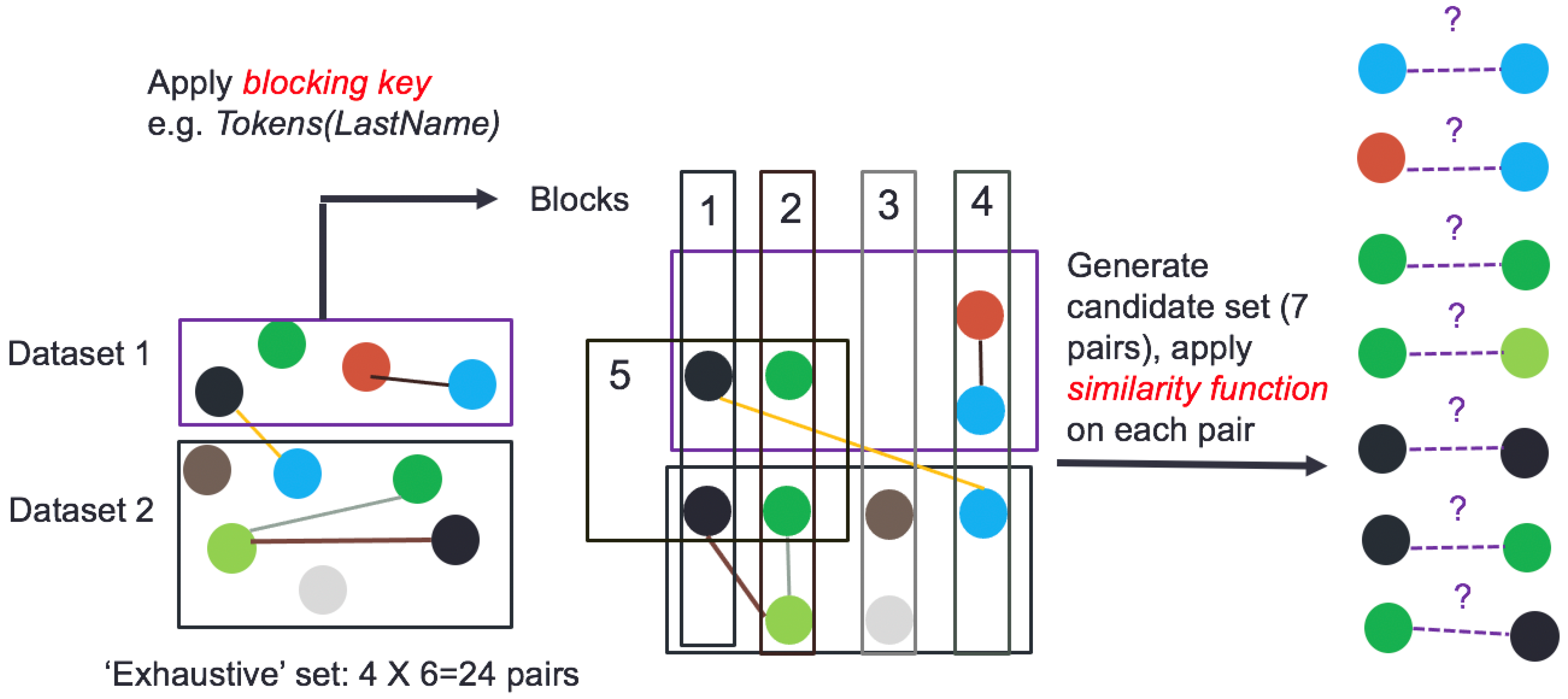
Entity Resolution (ER) is the identification of co-referent entities across datasets. Different communities refer to it as instance matching, record linkage, and the merge-purge problem [1,2]. Scalability indicates a two-step solution [1], as illustrated in Figure 1. The first step, blocking, mitigates brute-force pairwise comparisons on all entities by clustering entities into blocks and then comparing pairs of entities only within blocks [3]. For example, let us assume two knowledge graphs (KGs) describing customers (containing details, such as names, addresses and purchase histories) that must be linked. A blocking key, such as ‘Tokens(LastName)’, could first be applied to each node in the two KGs, as shown in the figure. In essence, this is a function that tokenizes the last name of each customer, and it assigns the customer to a block, indexed by the last-name token. According to the figure, this would lead to five overlapping blocks. One reason why blocks could overlap is that some customers may have multiple tokens in their last name e.g., Michael Ann-Moss.

Blocking results in the selection of a small subset of pairs, called the candidate set, which is input to a second step (called the ‘similarity’ step) to determine co-reference using a sophisticated similarity function. A good blocking key can lead to significant computational savings, as shown in the figure, while leading to minimal (or even no) loss of recall in the similarity step. While we exclusively address blocking in this work, we emphasize that it is only one part of a complete ER workflow. Pointers to the literature on the similarity step (that can often be applied independently of blocking) are provided in Section 2. We also provide background on the overall ER process, to place this work in context, in Section 3.

Blocking methods use a blocking scheme to assign entities to blocks. In some cases, blocking scheme and key are used interchangeably, but, typically, the former builds on the latter in a manner that we detail more formally in Section 4. Over the last two decades, Disjunctive Normal Form (DNF) Blocking Scheme Learners (BSLs) were proposed to learn DNF blocking schemes using supervised [4,5], semi-supervised [6], or unsupervised machine learning techniques [7]. DNF-BSLs have emerged as state-of-the-art, because they operate in an expressive hypothesis space and have demonstrated excellent empirical performance on real-world data [4]. Examples of DNF-BSLs will be provided in Section 4. However, despite their advantages, current DNF-BSLs assume that input datasets are tabular and have the same schemas. The latter assumption is often denoted as structural homogeneity [1]. Taking the earlier example of the customer domain, both of the datasets may rely on the same schema or ontology (also called a T-Box), which contains concepts such as Name, Address, Date, Credit Card Number, and so on, as well as properties such as name_of, lives_in, identified_by, and so on.

The assumption of tabular (or in the more general case of KGs, ontological) structural homogeneity restricts application of DNF-BSLs to other data models. The recent growth of heterogeneous KGs and ecosystems, such as the Linked Open Data [8] (in the Semantic Web community), motivates the development of a DNF-BSL for an arbitrary KG represented using the Resource Description Framework (RDF) data model. These graphs are often published by independent sources and are structurally heterogeneous [9]. Such KGs can make important contributions to multiple downstream search and recommendation applications, especially in e-commerce [10,11,12], but also in non-commercial domains, like building better systems for managing COVID-19 information overload, as evidenced by the success of the Google Knowledge Graph and the ongoing development of efforts such as the Amazon Product Graph [13,14,15]. However, without well-performing, efficient ER that works on structurally heterogeneous data, limited use can be made of publicly available KGs that are inexpensive to acquire and download, but have many redundancies and entity-overlap.

In this paper, we present a generic algorithmic pipeline for learning DNF blocking schemes on pairs of RDF KGs. The formalism of DNF blocking schemes relies on the existence of a schema. KGs, including RDF datasets published on the Web, may not have accompanying schemas [8], or in cases involving multiple KGs, may have different, independently developed schemas. Our proposed approach builds a dynamic schema using the properties in the KG. The KG dataset can then be logically represented as a property table, which may be populated at run-time. Previously, property tables were defined as physical data structures that were used in the implementation of triplestores [16]. By using a logical (rather than physical) property table representation, our approach admits the application of a DNF-BSL to RDF datasets, including KGs.

As a further special case, the pipeline also admits structurally heterogeneous tabular inputs. That is, the pipeline can be applied to tabular datasets with different schemas. Thus, previous DNF-BSLs become special cases of the pipeline, since they learn schemes on tables with the same schemas. As a second special case, the pipeline accommodates RDF-tabular heterogeneity, with one input, RDF, and the other, tabular. The utility of RDF-tabular heterogeneity is particularly apparent when linking datasets between Linked Open Data and the relational Deep Web [8,17]. The proposed method allows for us, at least in principle, to build efficient ER systems for doing so.

1.1. Contributions

Specific contributions in this article include:

• We formalize the problem of learning DNF blocking schemes on structurally heterogeneous datasets, including KGs and different-schema tabular dataset pairs.
• By way of an algorithmic solution, we present a generic pipeline for learning DNF blocking schemes. We also present an unsupervised instantiation of the generic pipeline by strategically employing an existing instance-based schema matcher called Dumas [18]. In addition to schema mappings, Dumas also generate noisy duplicates, which we recycle and pipe to a new DNF-BSL. The new DNF-BSL only uses two parameters, which may be robustly tuned for good empirical performance across multiple domains. The BSL is also shown to have a strong theoretical guarantee.
• We evaluate the full unsupervised pipeline on six real-world dataset pairs against two extended baselines, one of which is supervised [4,7]. Our system performance is found to be competitive, despite training samples not being manually provided. Given that unsupervised methods exist for the second ER step in both the Semantic Web and relational communities [1,2], this first unsupervised heterogeneous DNF-BSL enables, in principle, fully unsupervised ER in both communities.

1.2. Structure of the Article

The rest of the article proceeds, as follows. First, Section 2 describes some related work in the area, followed by background on the entire entity resolution process in Section 3. Preliminaries on blocking itself, as well as formalism, are covered in Section 4. Section 5 describes the generic pipeline, followed by an unsupervised instantiation in Section 6. Section 7 describes the experiments, with results and discussion in Section 8 and Section 9, respectively. The paper concludes (with some guidance on future work) in Section 10. A table with abbreviations and corresponding expanded forms, as well as an appendix with supplementary information, are also provided at the end of the work.

2. Related Work

Elmagarmid et al. comprehensively surveyed ER [1], with a generic approach represented by Swoosh [19]. Swoosh comprises a family of ER algorithms, including G-Swoosh, R-Swoosh, and F-Swoosh, with different theoretical guarantees and levels of expressiveness. However, Swoosh does not directly address the blocking problem.

A fairly recent survey on ER was provided in [20]. Within the ER community, blocking has separately witnessed much specific research, with Christen surveying numerous blocking methods [3], including traditional blocking and Sorted Neighborhood. In the specific research area of learning blocking schemes, which is what this work also builds on, Bilenko et al. [4] and Michelson and Knoblock [5] independently proposed the first supervised DNF-BSLs in 2006. Since then, a semi-supervised adaptation of the BSL proposed by Bilenko et al. has been published [4,6], as well as an unsupervised system [7]. The four systems assume structural homogeneity. We discuss their core principles in Section 5.3, and subsequently detail how the proposed approach generalizes them.

Since the advent of large knowledge graphs (KGs) on the Web [13,21,22], the problem of ER has taken on new urgency [23,24,25,26]. Recently, similarity techniques have become quite advanced, especially due to the rise of language representation models, such as BERT, GPT-3, and T5 [27,28,29], as well as so-called knowledge graph embeddings [30,31,32]. These models can be used to automatically ‘embed’ data items (including nodes, edges, words, or even sentences, depending on the model and input) into a continuous, low-dimensional, and real-valued vector space. Even using simple techniques, like logistic regression or cosine similarity (in the vector space), the vectors can be used to decide when two entities refer to the same underlying entity. Hence, the problem of feature engineering has largely been solved. However, because of the size of these KGs, blocking continues to be an important step, and research on blocking has lagged behind that of developing advanced similarity techniques. This paper is an attempt in that direction.

Heterogeneous blocking may be performed without learning a DNF scheme. One example is Locality Sensitive Hashing (LSH) [33,34], employed by the Harra system, for instance [35]. LSH is an algorithmic method that hashes similar inputs into the same ‘buckets’ with high probability. The efficacy of the algorithm depends on the precise definition of ‘similarity’ applied, and how high the similarity should be. With these caveats in place, an LSH ‘bucket’ could be thought of as a block. While LSH is promising, it only applies to specific distance measures, such as Jaccard and cosine distance (although recently, a measure was also proposed for the edit distance [36]). It is not clear how one would apply LSH to more complicated similarity functions, including machine learning classifiers.

Another good application of LSH for instance-based matching of large ontologies is [37]. The Typifier system by Ma et al. is an example that relies on type inferencing and it was designed for Web data published without semantic types [38]. In contrast, DNF-BSLs can be applied generally, with multiple studies showing strong empirical performance [4,5,6,7]. Other more recent blocking methods include methods, such as skyblocking [39], on top of which some recent work has also been developed [40]. In the skyblocking framework, each blocking scheme is mapped as a point to a multi-dimensional scheme space. The authors present efficient algorithms for learning such schemes. Finally, although related, clustering is technically treated separately from blocking in the literature [3]. However, recent approaches involving micro-clustering may show more promise for applying clustering methodologies to ER [41].

In the Semantic Web, ER is simultaneously known as instance matching and link discovery, and it has been surveyed by Ferraram et al. [2]. Existing work in the Semantic Web tends to restrict inputs to RDF. Also, most techniques in the Semantic Web do not learn schemes, but instead present graph-based blocking methods, with a good example being Silk [9]. Another recent method by Zhu et al. [25] uses unsupervised methods on multi-type graphs. Unfortunately, this method suffers from high complexity, and would likely benefit from the blocking methods described in this paper. In our own prior work, we have separately presented blocking methods for RDF graphs and for tables [7,26], but this is the first work to attempt to combine both types of inputs in a unified framework and demonstrate viable empirical performance on a range of datasets. A more theoretical treatment on graph-theoretic blocking schemes can be found in [42]. This article also significantly combines and builds on non-archival work by the author [42,43,44,45,46].

The framework in this paper also relies on schema mapping. Schema mapping is an active research area, with a good survey provided by Bellahsene et al. [47]. Gal notes that it is a difficult problem [48]. Schema matchers may return 1:1 or n:m mappings (or even 1:n and n:1). An instance-based schema matcher relies on data instances to perform schema matching [47]. A good example is Dumas [18], which relies on an inexpensive duplicates generator to perform unsupervised schema matching [18]. We describe Dumas in Section 6. An example of a related, and very recent, work that uses metadata (such as matching dependencies) to enhance the ER process is [49]. In principle, this work is similar to ours. The work by Caruccio et al. [50], while not directly about entity resolution, tackles the related problem of mining relaxed functional dependencies from data.

The property table representation used in this paper is a physically implemented data structure in the Jena triplestore API (https://jena.apache.org/, accessed on 18 March 2021), [16]. In this paper, it is used as a logical data structure. We note that the concept of logically representing one data model as another has precedent. In particular, literature abounds with proposed methods on how to integrate relational databases (RDB) with the Semantic Web. Sahoo et al. extensively surveyed this topic, called RDB2RDF [51]. A use-case is the Ultrawrap architecture, which utilizes RDB2RDF to enable real-time Ontology-based Data Access or OBDA [52]. We effectively tackle the inverse problem by translating an RDF graph to a logical property table. To our knowledge, this is the first application to devise such an inverse translation for heterogeneous ER.

3. Background: Two-Step Entity Resolution (ER)

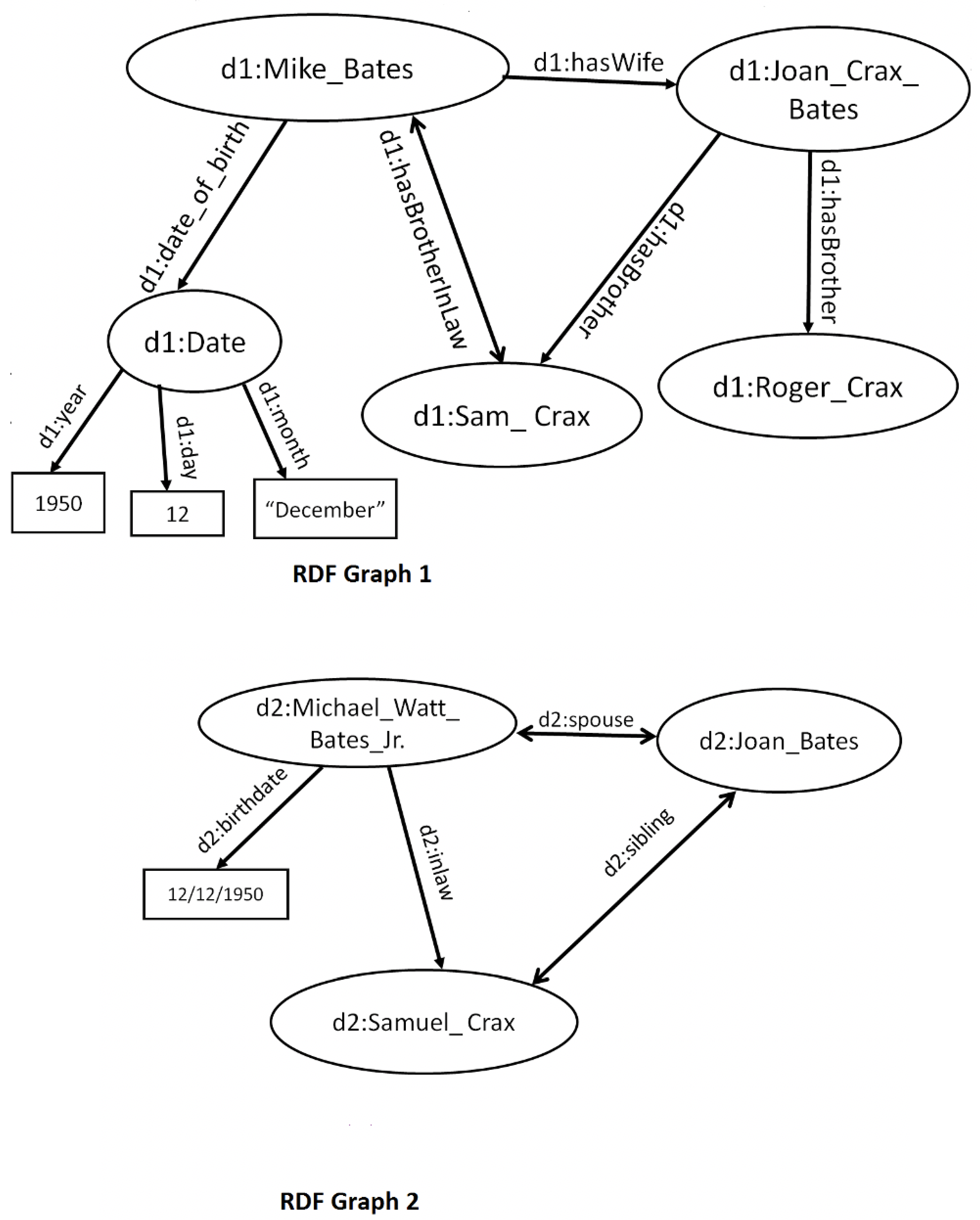
In this section, we begin with a conceptual background on ER. As defined earlier, ER is the problem of identifying pairs of entities across databases that refer to the same underlying entity. While an abstract example was provided earlier in Figure 1, a more concrete example is provided in Figure 2.

Given n entities and a boolean link specification or similarity function that determines whether two entities are equivalent, a naïve ER application would run in time $O\left(n^2\right)$. Even if we only limited comparisons between entities of the same type (e.g., Person-type entities would only be compared to other Person-type entities), there are still many unnecessary comparisons between the entities in Graphs 1 and 2 in Figure 2. If these graphs each contained thousands, or even millions of entities (which is not uncommon), the total number of pairwise comparisons would number in the trillions (${10}^6\times {10}^6$). Of course, in the worst case, if all entities were duplicates of one another, such comparisons are theoretically unavoidable. In practice, an entity in one knowledge graph is only linked to a small number (typically, far less than five even) of entities in the other knowledge graph. Therefore, for a million-node KG, the optimal number of similarity comparisons would be on the order of millions (the size of the KG), not trillions (the quadratic complexity). The question is, how do we discover most or all of the duplicate relationships while minimizing the number of comparisons, such that the number is closer to the optimal ($\approx O\left(n\right)$), rather than the exhaustive $O\left(n^2\right)$ number of necessary comparisons?

The ER community has converged on a set of techniques, called ‘blocking’, as an answer to this question. Early in the relational database community, for example, an algorithm called Sorted Neighborhood (SN) [53] would accept a rigidly structured tabular database as input, and sort the table by using a sorting key. For example, the table may be sorted on the basis of the ‘last name’ column, or even the date of birth. The idea was that records that were truly duplicates would be close to one another in the sorted table, assuming that the sorting key (also called a ‘blocking key’) was appropriate to begin with. A window of constant size is then slid over the records, and records sharing a window are paired and become candidates for the second ER step. This provably leads to an $O\left(n\right)$ complexity without significantly sacrificing the recall of duplicate detection.

In several studies, SN was verified to have excellent theoretical run-time guarantees and good empirical performance [3,53]. It had also been scaled to MapReduce and other highly parallel architectures [54]. However, it is not clear how the method can be obviously applied to graphs; another major problem is that the method assumes the provision of a sorting key, which is difficult to design from scratch, with guarantees. This paper is primarily concerned with the learning of such a blocking key, or its more generalized counterpart, called a blocking scheme. While previous work has shown how an expressive scheme can be learned given training data, our attempt relies on self-supervision to avoid the need for perfectly labeled training data. An added benefit is that the method also works for structurally heterogeneous datasets. In contrast, the majority of previous work in the blocking literature has tended to rely on the assumption of structural homogeneity, as we described earlier in Section 2, although more recent work has started lifting this assumption [26]. In the next section, we provide more formalism on blocking schemes and blocking scheme learning.

4. Preliminaries and Formalism

We present blocking-specific definitions and examples to place the remainder of the work in context. Consider a pair of datasets $R_1$ and $R_2$. Each dataset individually conforms to either the RDF or tabular data model. An RDF dataset may be visualized as a directed graph or equivalently, as a set of triples. A triple is a three-tuple of the form (subject, property, object). Note that a property is also called ‘predicate’ although we will continue to use ‘property’ for the purposes of uniformity. A tabular dataset conforms to a tabular schema, which is the table name followed by a set of fields. The dataset instance is a set of tuples, with each tuple comprising field values.

Example 1.

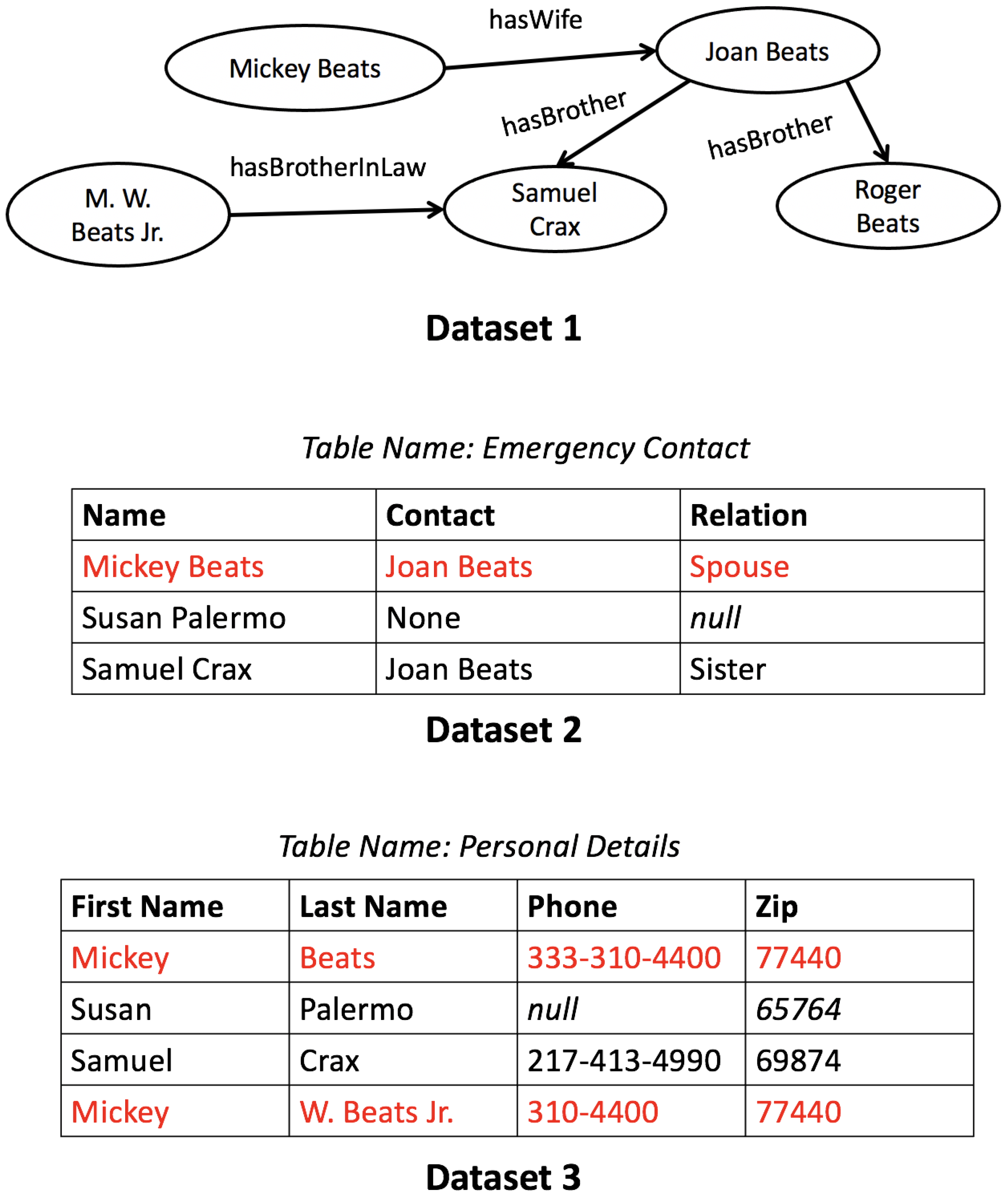
Dataset 1 (in Figure 3) is a more simplified version of the running example introduced earlier in Figure 2. It is an RDF dataset visualized as a directed graph $G=(V,E)$, and it can be equivalently represented as a set of $\left|E\right|$ triples. For example, (Mickey Beats, hasWife, Joan Beats) would be one such triple in the triples representation. Datasets 2 and 3 are tabular dataset examples, with the former having schema Emergency Contact(Name, Contact, Relation). The first tuple of Dataset 2 has field values Mickey Beats, Joan Beats, and Spouse, respectively. The keyword null is reserved. We will use the data in Figure 3 as the basis for our running examples in this section.

According to the RDF specification (http://www.w3.org/RDF/, accessed on 18 March 2021), subjects and properties must necessarily be Uniform Resource Identifiers (URIs), while an object node may either be a URI or a literal. URI elements in RDF files typically have associated names (or labels), obtained through de-reference. For ease of exposition, we henceforth refer to every URI element in an RDF file by its associated name. Additionally, note that in the most general case, RDF datasets do not have to conform to any schema. This is why they are commonly visualized as semi-structured datasets, and not as tables. In Section 5.1, we show how to dynamically build a property schema and logically represent RDF as a tabular data structure.

An entity is defined as a semantically distinct subject node in an RDF dataset, or as a (semantically distinct) tuple in a tabular dataset. The entity referring to Mickey Beats is shown in red in all datasets in Figure 3. In this context, ER is the process of resolving semantically equivalent (but possibly syntactically different) entities. As earlier described, the majority of ER research has traditionally assumed structural homogeneity, an example of which would be identifying that the two highlighted tuples in Dataset 3 are duplicates.

In the Semantic Web, ER is operationalized by connecting two equivalent entities with an owl:sameAs (http://www.w3.org/TR/owl-ref/, accessed on 18 March 2021), property edge. For example, the two nodes referring to Mickey Beats in Dataset 1 should be connected while using an owl:sameAs edge. Easy operationalizing of ER (and more generally, ‘link specification’ [9]) explains in part the ongoing interest in ER in the Semantic Web [2]. In the relational setting, ER is traditionally operationalized through joins or mediated schemas. It is less evident how to operationalize ER across RDF-tabular inputs, such as linking Datasets 1 and 2. We return to this issue in Section 5.1.

In order to introduce the current notion of DNF blocking schemes, tabular structural homogeneity is assumed for the remainder of this section. In later sections, we generalize the concepts as a core contribution of this paper.

The most basic elements of a blocking scheme are indexing functions $h_i\left(x_t\right)$ [4]. An indexing function accepts a field value from a tuple as input and returns a set Y that contains 0 or more blocking key values (BKVs). A BKV identifies a block in which the tuple is placed. Intuitively, one may think of a block as a hash bucket, except that blocking is one-many while hashing is typically many-one [3]. For example, if Y contains multiple BKVs, then a tuple is placed in multiple blocks.

Definition 1.

An indexing function $h_i:Dom\left(h_i\right)\to U^{\ast }$ takes as input a field value $x_t$ from some tuple t and returns a set Y that contains 0 or more Blocking Key Values (BKVs) from the set of all possible BKVs $U^{\ast }$.

The domain $Dom\left(h_i\right)$ is usually just the string datatype. The range is a set of BKVs that the tuple is assigned to. Each BKV is represented by a string identifier.

Example 2.

An example of an indexing function is Tokens. When applied to the Last Name field value of the fourth tuple in Dataset 3, the output set Y is $\{W.,Beats,Jr.\}$.

This leads to the notion of a general blocking predicate (GBP). Intuitively, a GBP $p_i(x_{t_1},x_{t_2})$ takes as input field values from two tuples, $t_1$ and $t_2$, and uses the ith indexing function to obtain BKV sets $Y_1$ and $Y_2$ for the two arguments. The predicate is satisfied if $Y_1$ and $Y_2$ share elements, or equivalently, if $t_1$ and $t_2$ have a block in common.

Definition 2.

A general blocking predicate $p_i:Dom\left(h_i\right)\times Dom\left(h_i\right)\to \{True,$ $False\}$ takes as input field values $x_{t_1}$ and $x_{t_2}$ from two tuples, $t_1$ and $t_2$, and returns True if $h_i\left(x_{t_1}\right)\cap h_i\left(x_{t_2}\right)\ne \Phi$, and returns False otherwise.

Each GBP is always associated with an indexing function.

Example 3.

Consider the GBP ContainsCommonToken, associated with the previously introduced Tokens. Suppose that it was input the Last Name field values from the first and fourth tuples in Dataset 3. Because these field values have a token (Beats) in common, the GBP returns True.

A specific blocking predicate (SBP) explicitly pairs a GBP to a specific field.

Definition 3.

A specific blocking predicate is a pair $(p_i,f)$, where $p_i$ is a general blocking predicate and f is a field. A specific blocking predicate takes two tuples $t_1$ and $t_2$ as arguments and applies $p_i$ to the appropriate field values $f_1$ and $f_2$ from both tuples. A tuple pair is said to be covered if the specific blocking predicate returns True for that pair.

Previous DNF research assumed that all available GBPs can be applied to all fields of the relation [4,5,6,7]. For this reason, they were neither obviously applicable to different-schema relational databases, nor to knowledge graphs. Hence, given a relation R with m fields in its schema, and s GBPs, the number of SBPs is exactly $ms$. Note that structural homogeneity implies exactly one input schema, even if there are multiple relational instances. Finally, a DNF blocking scheme is defined as:

Definition 4.

A DNF blocking scheme $f_P$ is a positive propositional formula constructed in Disjunctive Normal Fo-rm or DNF (a disjunction of terms, where each term is a conjunction of literals), using a given set H of SBPs as the set of atoms. Additionally, if each term is constrained to comprise at most one atom, then the blocking scheme is referred to as disjunctive.

SBPs cannot be negated, since the DNF scheme is a positive formula. A tuple pair is said to be covered if the blocking scheme returns True for that pair. Intuitively, this means that the two constituent tuples share a block. In practice, both duplicate and non-duplicate tuple pairs can end up getting covered, since blocking is just a pre-processing step.

Example 4.

Consider the disjunctive scheme (ContainsCommonToken, Last Name) ∨ (SameFirstDigit, Zip), applied on Dataset 3. While the two tuples referring to Mickey Beats would share a block (with the BKV Beats), the non-duplicate tuples referring to Susan and Samuel would also share a block (with the BKV 6). Additionally, note that the first and fourth tuples share more than one block, since they also have BKV 7 in common.

Given a blocking scheme, a blocking method would need to map tuples to blocks efficiently. According to the definition provided earlier, a blocking scheme takes a tuple pair as input. In practice, linear-time hash-based techniques are usually applied.

Example 5.

To efficiently apply the blocking scheme in the previous example on each individual tuple, tokens from the field value corresponding to field Last Name are extracted, along with the first character from the field value of the Zip field, to obtain the tuple’s set of BKVs. For example, being applied to the first tuple of Dataset 3, the BKV set $\{Beats,7\}$ is extracted. An index is maintained, with the BKVs as keys and tuple pointers as values. With n tuples, traditional blocking computes the blocks in time $O\left(n\right)$ [3].

Let the set of generated blocks be $\Pi$. $\Pi$ contains sets of the form $B_v$, where $B_v$ is the block that is referred to by the BKV v. The candidate set of pairs $\Gamma$ is given below:

$$\Gamma =\bigcup _{B_v\in \Pi }\left\{(r,s)\right\},\forall r,s\in B_v|r\in R_1,s\in R_2$$

(1)

$\Gamma$ is precisely the set input to the second step of ER, which classifies each pair as a duplicate, non-duplicate, or probable duplicate [55]. Blocking should produce a small $\Gamma$ but with high coverage and density of duplicates. Metrics quantifying these properties are defined in Section 7.

Finally, schema mapping is utilized in the paper. The formal definition of a mapping is quite technical; the survey by Bellahsene et al. provides a full treatment [47]. In this paper, an intuitive understanding of the mapping as a pair of field-sets suffices. For example, ({Name},{First Name, Last Name}) is a 1:n mapping between Datasets 2 and 3. More generally, mappings may be of cardinality n:m. The simplest case is a 1:1 mapping, with singleton components.

5. The Generic Pipeline

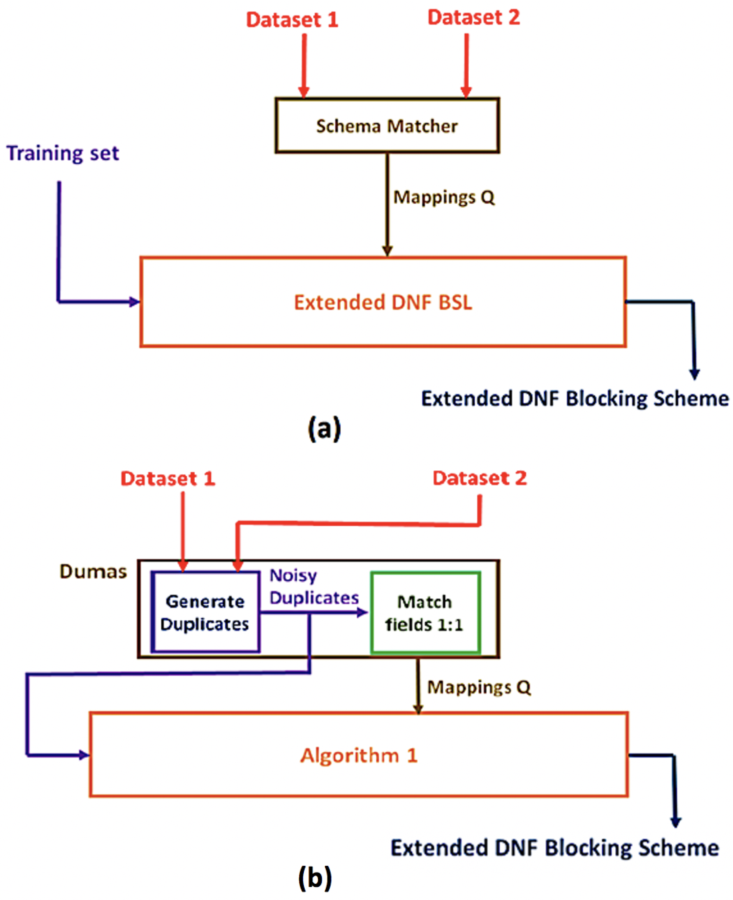
Figure 4a shows a schematic of a generic pipeline for DNF blocking scheme learning on heterogeneous datasets. Specifically, two heterogeneous datasets are initially provided as input, with either dataset being RDF or tabular. If the dataset is RDF, then we logically represent it as a property table. We describe the details and advantages of this tabular data structure in Section 5.1. The key point to note is that the schema matching module takes two tables as input, regardless of the data model, and outputs a set of schema mappings Q. An extended DNF-BSL accepts Q and also a training set of duplicates and non-duplicates as input, and learns an extended DNF blocking scheme. The DNF-BSL and blocking scheme need to be extended, because tables are now structurally heterogeneous, and the Section 4 formalism does not natively apply. In Section 5.2, the formalism is extended to admit structural heterogeneity. Figure 4b shows an unsupervised instantiation of the generic pipeline. We describe the details in Section 6.

5.1. Property Table Representation

Despite their formal description as sets of triples, RDF files are often physically stored in triplestores as sparse property tables [16]. In this paper, we adapt this table instead as a logical tabular representation of RDF. To enable the logical construction on RDF dataset R, we define the property schema $\left\{subject\right\}\cup \left\{p\right|\exists (s,p,o),(s,p,o)\in R\}$. In essence, we flatten the graph by assigning each distinct property (or edge label) a corresponding field in this schema, along with an extra subject field. Every distinct subject in the triples-set has exactly one corresponding tuple in the table.

For example, Figure 5 is the property table representation of Dataset 1 in Figure 3. If a subject does not have a corresponding object value for a given property, then the reserved keyword null is entered. If a subject has multiple object values for a property, the values are concatenated using a reserved delimiter; (in Figure 5). Technically, the field values now have set semantics, with null representing the empty set. Additionally, the original set of triples can be losslessly reconstructed from the property table (and vice versa), making it an information-preserving logical representation. Although intuitively straightforward, we detail these lossless conversions in the Appendix A.

The physical property table was proposed to eliminate expensive property-property self-joins that occur frequently in SPARQL (http://www.w3.org/TR/rdf-sparql-query/, accessed on 18 March 2021) queries. For ER, the logical data structure is useful, because it allows for a dynamic schema that is resolvable at run-time. Triplestores, like Jena, allow updating and querying of RDF graphs, despite the underneath tabular representation [16]. If the RDF dataset is already stored in such a triplestore, then it would not have to be moved prior to ER. This gives the property table a systems-level advantage.

More importantly, having a schema for an RDF dataset means that we can invoke a suitable schema matcher in the generalized pipeline. As we subsequently show, the extended DNF-BSL in the pipeline requires the datasets to have (possibly different) schemas. Finally, representing RDF as a table allows for us to address RDF-tabular heterogeneity, by reducing it to tabular structural heterogeneity. Traditional ER operations become well-defined for RDF-tabular inputs.

One key advantage of the property schema is that it does not rely on RDF Schema (RDFS) metadata. In practice, this allows for us to represent any file on Linked Open Data tabularly, regardless of whether metadata are available.

Even in the simple example of Figure 5, we note that the property table is not without its challenges. It is usually sparse, and it may end up being broad, for RDF datasets with many properties. Furthermore, properties are named using different conventions (for example, the prefix Has occurs in all the properties in Figure 5) and it could be opaque, depending on the dataset publisher. We empirically show (Section 7) that the instantiated pipeline (Section 6) can handle these difficulties.

5.2. Extending the Formalism

The formalism in Section 4 assumed structural homogeneity. We extend it to accommodate structural heterogeneity. As input, consider two datasets $R_1$ and $R_2$. If either dataset is in RDF, we assume that it is in property table form. Recall the original definition of SBPs provided earlier. SBPs are associated with a single GBP and a single field, making them amenable only to a single schema. To account for heterogeneity, we extend SBPs by replacing the field input with a mapping. Denote, as $A_1$ and $A_2$, the respective sets of fields of datasets $R_1$ and $R_2$. We define simple extended SBPs below:

Definition 5.

A simple extended specific blocking predicate is a pair $(p_i,m)$ where $p_i$ is a general blocking predicate and $m=(\left\{f_1\right\},\left\{f_2\right\})$ is a mapping from a single field $f_1\in A_1$ to a single field $f_2\in A_2$. The predicate takes two tuples $t_1$ and $t_2$ as arguments and applies $p_i$ to the field values corresponding to $f_1$ and $f_2$ in the two tuples, respectively.

The correspondence in this definition is denoted as simple, since it uses a mapping of the simplest cardinality (1:1). The earlier definition of a specific blocking predicate can be reformulated as a special case of the stated definition, with $A_1=A_2$ and $f_1=f_2$.

The SBP semantics are not evident if the mapping cardinality is n:m, 1:n or n:1, which is, between two arbitrary field-subsets, $F_1\subseteq A_1$ and $F_2\subseteq A_2$. If we interpret the two sets as representing $|F_1\left|\right|F_2|$ 1:1 mappings, then we obtain a set of simple extended SBPs $\left\{(p_i,(\left\{f_1\right\},\left\{f_2\right\}))\right|f_1\in F_1,f_2\in F_2\}$.

The interpretation above is motivated by the requirement that an SBP should always return a boolean value. We approach the problem by using the n:m mappings to construct the set of simple extended SBPs, as shown above. We then use disjunction as a combine operator on all elements of the constructed set to yield a single boolean result. We can then define complex extended SBPs.

Definition 6.

A complex extended specific blocking predicate is a pair $(p_i,M)$ where $p_i$ is a general blocking predicate and M is a mapping from a set $F_1\subseteq A_1$ to a set $F_2\subseteq A_2$. The predicate takes two tuples $t_1$ and $t_2$ as arguments and then applies on them $|F_1\left|\right|F_2|$ simple extended SBPs $(p_i,m)$, where m ranges over all 1:1 mappings in the set $\left\{(\left\{f_1\right\},\left\{f_2\right\})\right|f_1\in F_1,f_2\in F_2\}$. The predicate returns the disjunction of these $|F_1\left|\right|F_2|$ values as the final output.

Example 6.

Consider the mapping between sets {Name} in Dataset 2 and {First Name, Last Name} in Dataset 3, in Figure 3. Let the input GBP be ContainsCommonToken. The complex extended SBP corresponding to these inputs would be ContainsCommonToken({Name}, {First Name}) ∨ ContainsCommonToken({Name}, {Last Name}). This complex extended SBP would yield the same result as the simple extended SBP ContainsCommonToken({Na-me},{Name}) if a new field called Name is derived from the merging of the First Name and Last Name fields in Dataset 3.

An operator, like conjunction, is theoretically possible, but it may prove restrictive when learning practical schemes. The disjunction operator makes complex extended SBPs more expressive than simple extended SBPs, but it requires more computation (Section 5.3). Evaluating alternate combine operators is left for future work.

Finally, (simple or complex) extended DNF schemes can be defined in a similar vein as the earlier definition on DNF blocking schemes, using (simple or complex) extended SBPs as atoms. One key advantage of using disjunction as the combine operator in Definition 6 is that, assuming simple extended SBPs as atoms for both simple and complex extended DNF schemes, the scheme remains a positive boolean formula, by virtue of the distributivity of conjunction and disjunction.

5.3. Extending Existing DNF-BSLs

Existing DNF-BSLs [4,5,6,7] rely on similar high-level principles, which is to devise an approximation algorithm for solving the NP-hard optimization problem that was first formalized by Bilenko et al. [4]. The approximation algorithms are different, in that they require different parameters and levels of supervision. These are detailed below and summarized in

Table 1. Disjunctive Normal Form Blocking Scheme Learner (DNF-BSL) Systems.

ID	System	Parameters	Supervision
1	Michelson and Knoblock [5]	$ϵ$, k	Supervised
2	Bilenko et al. [4]	$ϵ$, $\eta$, k	Supervised
3	Cao et al. [6]	s, $ϵ$, $\tau$, $\alpha$, k	Semi-supervised
4	Kejriwal and Miranker [7]	Generator: c, $ut$, $lt$, d, $nd$; Learner: $ϵ$, $\eta$, k	Unsupervised
5	Algorithm 1 herein	$\kappa$, k	Unsupervised

. These BSLs were only originally designed for structurally homogeneous tables, with a single field-set A. We describe their underlying core principles before describing extensions in keeping with the formalism in Section 5.2.

Assume a set of GBPs G. The core of all approximation algorithms would first construct a search space of SBPs H by forming the cross product of G and A. The goal of the algorithm is to choose a subset $H^{\prime }\subseteq H$, such that the optimization condition (we describe the condition here intuitively, and formally state it in the Appendix A). laid out by Bilenko et al. is satisfied, at least approximately [4]. The condition assumes that training sets of duplicates D and non-duplicates N are provided. Intuitively, the condition states that the disjunctive blocking scheme that formed by taking the disjunction of SBPs in $H^{\prime }$ covers (see Definition 4) at least $ϵ\left|D\right|$ duplicates, while covering the minimum possible non-duplicates [4]. Note that $ϵ$ is a parameter that is common to all four systems ($ϵ$ was designated as min_thresh in the original System 1 paper [5], and $\sigma$ in the System 3 paper [6]) in Table 1.

A beam search parameter k (also common to all four systems) is required in order to learn a DNF scheme (as opposed to just disjunctive). This parameter is used to supplement the original set H with terms, to obtain a new set $H_c$. Figure 6 demonstrates this combinatorial process.

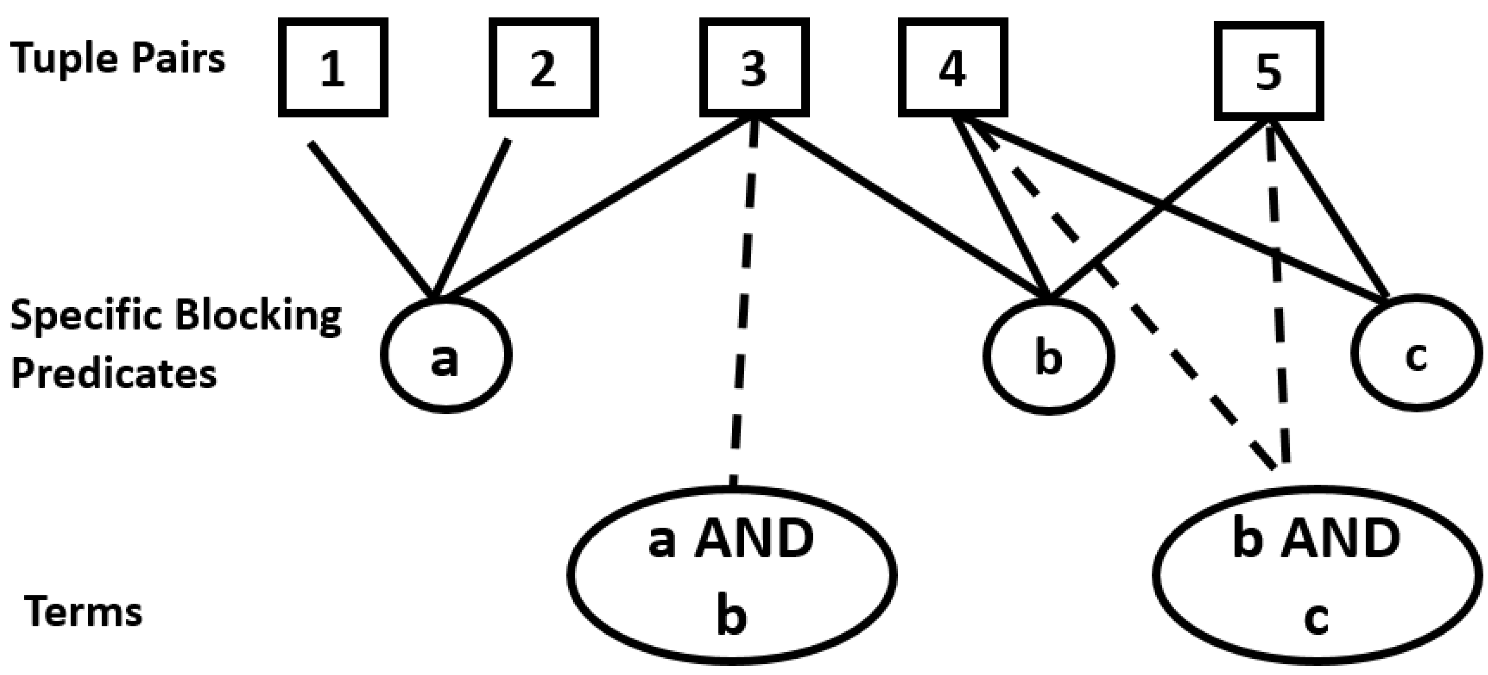
H originally consists of the SBPs a, b and c. These SBPs cover some tuple pairs (TPs). Suppose that $k=2$. A term of size 2 is formed by checking if any TP is covered by (at least) two SBPs. For example, TP-3 is covered by SBPs a and b and, hence, also covered by the term $a\wedge b$. For $k>2$, terms from size 2 to size k are recursively added to H; the final supplemented set is denoted as $H_c$. Note that for $\left|H\right|$ predicates, building $H_c$ takes $O\left(\right|H{|}^k)$ time per TP. Given the exponential dependence on k and diminishing returns, the previous results capped k at 2 [4,7]. If $k=1$, $H_c=H$.

The set $H^{\prime }\subseteq H_c$ that is now chosen by the approximation scheme would potentially consist of terms and SBPs, with their disjunction yielding a k-DNF scheme. A k-DNF formula has at most k literals in each term.

While System 1 only requires $ϵ$ and k as its parameters, Systems 2 and 4 prune their search spaces by removing all SBPs and terms from $H_c$ that cover more than $\eta \left|N\right|$ non-duplicates. Note that this step heuristically improves both (because $H_c$ now contains only a few, high-quality elements) quality and run-time. It comes at the risk of failure, since if the search space is pruned excessively (by high $\eta$), it may become impossible to cover at least $ϵ\left|D\right|$ duplicates. Systems 3 and 4 require less supervision, but significantly more parameter tuning, given they rely on many more parameters.

Systems 1–3 rely on different (surveyed briefly in the Appendix A) Set Covering (SC) variants [56]. All three systems can be extended by constructing a search space of complex extended SBPs using G and the mappings set Q, instead of G and a field set A. The underlying SC approximations operate in this abstract search space to choose the final set $H^{\prime }$. An extended DNF scheme is formed by a disjunction of (extended) elements in $H^{\prime }$.

Modifying System 4 is problematic because the system is unsupervised and runs in two phases. The first phase (denoted as generator) generates a noisy training set, and the second phase (denoted learner) performs feature-selection on the noisy set to output a DNF blocking scheme. The feature-selection based learner is similar to Systems 1–3 and can be extended. Unfortunately, the generator explicitly assumes homogeneity, and it cannot be directly extended to generate training examples for heterogeneous datasets. This implies that the DNF-BSL component of the proposed generic pipeline in Figure 4a cannot be instantiated with an existing unsupervised system.

In the event that a schema matcher (and, thus, Q) is unavailable in Figure 4a, we present a fall-back option. Specifically, we build a set Q of all 1:1 mappings, $\left|Q\right|=|A_1\left|\right|A_2|$. Recall that $A_i$ is the field set of dataset i. We denote the constructed set H of SBPs as simple exhaustive. Note that for the set of all mappings ($\approx 2^{|A_1|}{2}^{|A_2|}$), the constructed set H (denoted complex exhaustive) is not computationally feasible for non-trivial cases. Even the simple exhaustive case is only a fall-back option, since a true set of 1:1 mappings Q would be much smaller (at most min($|A_1|,|A_2|$)) than this set.

6. An Unsupervised Instantiation

A key question addressed in this work is whether the generic pipeline can be instantiated in an unsupervised fashion. As we showed earlier, existing DNF-BSLs that can be extended require some form of supervision. An unsupervised heterogeneous DNF-BSL is important because, in principle, it enables a fully unsupervised ER workflow in both the relational and Semantic Web communities. As the surveys by Elmagarmid et al. and Ferraram et al. note, unsupervised techniques for the second ER step do exist already [1,2]. A second motivation is the observation that existing unsupervised and semi-supervised homogeneous DNF-BSLs (Systems 3–4) require considerable parameter tuning. Parameter tuning is being increasingly cited as an important algorithmic issue, in applications ranging from schema matching [57] to generic machine learning [58]. Variety in Big Data implies that algorithm design cannot discount parameter tuning.

We propose an unsupervised instantiation with a new DNF-BSL that only requires two parameters. In Table 1, only the supervised System 1 requires two parameters. The schematic of the unsupervised instantiation (of the generic pipeline in Figure 4a) is shown in Figure 4b. We use the existing schema matcher, Dumas, in the instantiated pipeline [18]. Dumas outputs 1:1 field mappings by first using a duplicates generator to locate tuple pairs with high cosine similarity. In the second step, Dumas uses Soft-TFIDF to build a similarity matrix from each generated duplicate. If n duplicates are input to the second step, then n similarity matrices are built and then averaged into a single similarity matrix. The assignment problem is then solved by invoking the Hungarian Algorithm on this matrix [59]. This results in exactly $min\left(\right|A_1|,|A_2\left|\right)$ 1:1 field mappings (the set Q) being output.

In addition to using Q, we recycle the noisy duplicates of Dumas and then pipe them into Algorithm 1. Note that Dumas does not generate non-duplicates. We address this issue in a novel way, by permuting the generated duplicates set D. Suppose that D contains n tuple pairs $\{(r_1,s_1),\dots (r_n,s_n)\}$, with each $r,s$, respectively, from datasets $R_1,R_2$. By randomly permuting the pairs in D, we heuristically obtain non-duplicate pairs of the form $(r_i,s_j)$, $i\ne j$. Note that (at most) $n!$ distinct permutations are possible. For balanced supervision, we set $\left|N\right|=\left|D\right|$, with N the permutation-generated set.

Algorithm 1 Learn Extended k-DNF Blocking Scheme.

Input: Set D of duplicate tuple pairs, Set Q of mappings Parameters: Beam search parameter k, SC-threshold $\kappa$ Output: Extended DNF Blocking Scheme $\mathcal{B}$ Method://Step 0: Construct sets N and H 1. Permute pairs in D to obtain N, $\left|N\right|=\left|D\right|$ 2. Construct set H of simple extended SBPs using set G of GBPs and Q 3. Supplement set H to get set $H_c$ using k //Step 1: Build Multimaps $M_D^{\prime }$ and $M_N^{\prime }$ 4. Construct $M_D=<X,H_X>$, X is a tuple pair in D, $H_X\subseteq H_c$ contains the elements in $H_c$ covering X 5. Repeat previous step to build $M_N$ for tuple pairs in N 6. Reverse $M_D$ and $M_N$ to respectively get $M_D^{\prime }$ and $M_N^{\prime }$ //Step 2: Run approximation algorithm for all$X\in keyset\left(M_D^{\prime }\right)$do  8. Score X by using formula $|M_D^{\prime }\left(X\right)|/|D|-|M_N^{\prime }\left(X\right)|/|N|$  9. Remove X if $score\left(X\right)<\kappa$ end for 11. Perform W-SC on keys in $M_D^{\prime }$ using Chvatal’s heuristic, weights are negative scores //Step 3: Construct and output DNF blocking scheme 12. $\mathcal{B}:=$ Disjunction of chosen keys 13. Output $\mathcal{B}$

Empirically, the permutation is expected to yield a precise N because of observed duplicates sparsity in ER datasets [3,7]. This sparsity is also a key tenet underlying the blocking procedure itself. If the datasets were dense in duplicates, blocking would not yield any savings.

Algorithm 1 shows the pseudocode of the extended DNF BSL. Inputs to the algorithm are the piped Dumas outputs, D and Q. To learn a blocking scheme from these inputs, two parameters, k and $\kappa$, beed to be specified. Similar to (extended) Systems 1–3 in Table 1, G, Q, and k are used to construct the search space, $H_c$. Note that G is considered the algorithm’s feature space, and it is not a dataset-dependent input (or parameter). Designing an expressive G has computational and qualitative effects, as we empirically demonstrate. We describe the GBPs that are included in G in Section 7.

Step 0 in Algorithm 1 is the permutation step just described to generate the non-duplicates set N. G and Q are then used to construct the set H of simple extended (because Dumas only outputs 1:1 mappings) SBPs, with $\left|H\right|=\left|G\right|\left|Q\right|$. H is supplemented (using parameter k) to yield $H_c$, as earlier described in Section 5.3.

Step 1 constructs multimaps (multimap keys reference multiple values, or a value set) on which Set Covering (SC) is eventually run. As a first logical step, multimaps $M_D$ and $M_N$ are constructed. Each tuple pair (TP) in D is a key in $M_D$, with the SBPs and terms in $H_c$ covering that TP comprising the value set. $M_D$ is then reversed to yield $M_D^{\prime }$. $M_N^{\prime }$ is built analogously. Figure 7 demonstrates the procedure, assuming that D contains TPs 1-5, covered as shown in Figure 6. The time complexity of building (both) $M_D^{\prime }$ and $M_N^{\prime }$ is ${O\left(\right|H|}^k\left(\right|D|+\left|N\right|\left)\right)$.

In Step 2, each key is first scored by calculating the difference between the fractions of covered duplicates and non-duplicates. A threshold parameter, $\kappa$, is used to remove the SBPs and terms that have low scores. Intuitively, $\kappa$ tries to balance the conflicting needs of previously described parameters, $ϵ$ and $\eta$, and reduce tuning effort. The range of $\kappa$ is [−1, 1]. An advantage of the parameter is that it has an intuitive interpretation. A value that is close to $1.0$ would indicate that the user is confident about low noise-levels in inputs D and Q, since high $\kappa$ implies the existence of elements in $H_c$ that cover many positives and few negatives. Because many keys in $M_D^{\prime }$ are removed by high $\kappa$, this also leads to computational savings. However, setting $\kappa$ too high (perhaps because of misguided user confidence) could potentially lead to excessive purging of $M_D^{\prime }$, and subsequent algorithm failure. Experimentally, we show that $\kappa$ is easily tunable and even high values of $\kappa$ are robust to noisy inputs.

Weighted Set Covering (W-SC) is then performed using Chvatal’s algorithm (we include Chvatal’s algorithm in the Appendix A.3 survey) [56], with each key in $M_D^{\prime }$ acting as a set and the tuple pairs covered by all keys as elements of the universe set $\mathcal{U}$. For example, assuming that all SBPs and terms in the keyset of $M_D^{\prime }$ in Figure 7 have scores above $\kappa$, $\mathcal{U}=\{1,2,3,4,5\}$. Note that only $M_D^{\prime }$ is pruned (using $\kappa$) and, also, W-SC is performed only on $M_D^{\prime }$. $M_N^{\prime }$ only aids in the score calculation (and subsequent pruning process) and may be safely purged from memory before W-SC commences.

W-SC needs to find a subset of the $M_D^{\prime }$ keyset that covers all of $\mathcal{U}$ and with minimum total weight. For this reason, the weight of each set is the negative of its calculated score. Given that sets chosen by W-SC actually represent SBPs or terms, their disjunction is the k-DNF blocking scheme.

Under plausible (essentially, assuming that $P\subset NP$) complexity assumptions, Chvatal’s algorithm is essentially the best-known polynomial-time approximation for W-SC [60]. For example, Bilenko et al. used Peleg’s approximation to Red-Blue SC [61,62], which is known to have worse bounds [62]. The proposed DNF-BSL has the strongest theoretical approximation guarantee of all systems in Table 1.

7. Experiments

7.1. Metrics

The quality and efficiency of blocking is evaluated by the special metrics, Reduction Ratio (RR), Pairs Completeness (PC), and Pairs Quality (PQ) [3]. Traditional metrics like precision and recall do not apply to blocking since it is a pre-processing step, and its output is not the final ER output.

To define RR, which intuitively measures efficiency, consider the full set of pairs $\Omega$ that would be generated in the absence of blocking. Specifically, $\Omega$ is the set $\left\{(r,s)\right|r\in R_1,s\in R_2\}$. RR is then given by the formula:

$$RR=1-|\Gamma |/|\Omega |$$

(2)

Given the sparsity of duplicates in real-world datasets [3], RR should ideally be close to, but not precisely, $1.0$ (unless $\Gamma =\varphi$).

Let us denote the set of all duplicate pairs, or the ground-truth, as ${\Omega }_m$. Similarly, consider the set of duplicates included in the candidate set ${\Gamma }_m=\Gamma \cap {\Omega }_m$. The metric PC quantifies the effectiveness of the blocking scheme by measuring coverage of ${\Gamma }_m$ with respect to ${\Omega }_m$. Specifically, it is given by the formula:

$$PC=|{\Gamma }_m|/|{\Omega }_m|$$

(3)

Low PC implies that recall on overall ER will be low, since many duplicates did not share a block to begin with.

PC and RR together express an efficiency-effectiveness tradeoff. The metric PQ is sometimes used to measure how dense the blocks are in duplicates, and it is given by:

$$PQ=|{\Gamma }_m|/|\Gamma |$$

(4)

PQ has not been reported in recent BSL literature [4,7]. One reason is that PQ can be equivalently expressed as $c.PC/(1-RR)$, where c is $|{\Omega }_m|/|\Omega |$. When comparing two BSLs, PQ can therefore be expressed wholly in terms of PC and RR. We do not consider PQ further in this paper.

7.2. Evaluating Dumas Using Preliminary Experiments

Given that the test suite is larger and more heterogeneous in this paper than in the original Dumas work [18], we perform two preliminary experiments to evaluate Dumas before describing the experimental study and methodology behind the core DNF-BSL algorithm that was presented earlier. Dumas was briefly described in Section 6.

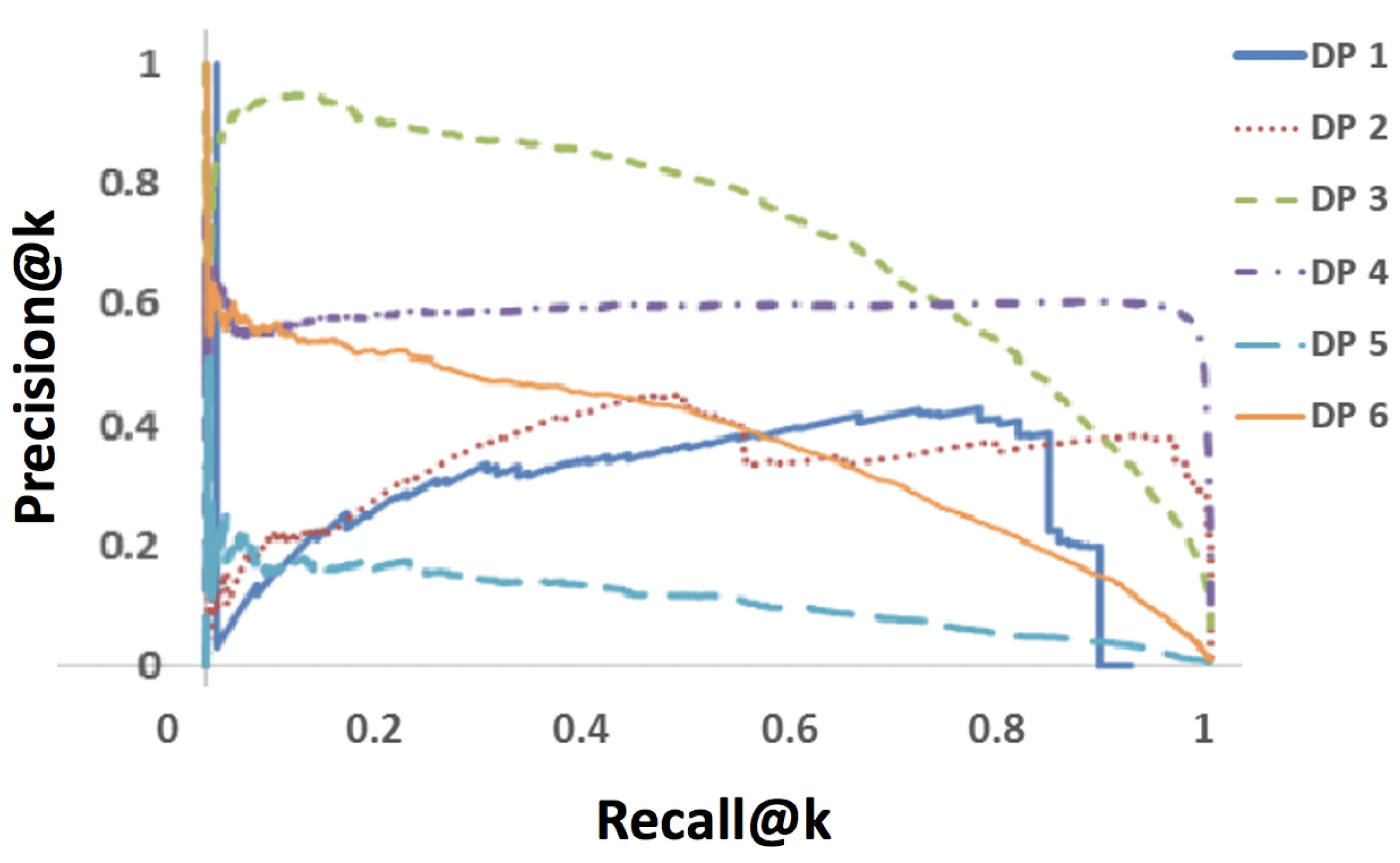
For the first preliminary experiment, we evaluate the performance of Dumas’s duplicates generator. The generator uses TF-IDF to retrieve the highest scoring duplicates in order. Suppose that we retrieve t duplicates (as an ordered list). Denote, for any $k\le t$, the number of true positives in sub-list $[1\dots k]$ as $d\left(k\right)$. Define Precision@k as $d\left(k\right)/k$ and Recall@k as $d\left(k\right)/|{\Omega }_m|$, where ${\Omega }_m$ is the ground-truth set of all duplicates. We plot Precision@k against Recall@k for all DPs to demonstrate the precision-recall tradeoff. To obtain a full set of data points, we set t at 50,000 for all experiments, and calculate Precision@k and Recall@k for $k\in \{1\dots t\}$.

Figure 8 shows the results of Dumas’ duplicates-generator on all six dataset pairs (DPs) that were used for evaluation (that we profile in Section 7.4). Except for DP 3, precision on all cases seems inadequate, even at low recall levels. Although recall of 100% is eventually attained on most DPs, the price is (near) 0% precision. A closer inspection of the results showed that many false positives got ranked at the top. We discuss the implications of these noisy results shortly.

For the second preliminary experiment, we attempt to evaluate Dumas’ schema matching performance. Although t was set to a high value in the previous experiment, Dumas only requires a few top pairs (typically 10–50) for the schema matching step [18]. To compute the similarity matrix from t pairs, Dumas uses Soft TF-IDF, which requires an optional threshold $\theta$. For a given DP, denote $Q^{\prime }$ as the ground-truth set of schema mappings, Q as the set of Dumas mappings, and $Q_m\subseteq Q$ as the set of correct Dumas mappings. Define precision (on this task) as $|Q_m|/|Q|$ and recall as $|Q_m|/|Q^{\prime }|$.

We set t and $\theta$ to default values of 50 and $0.5$, respectively, and report the results in

Table 2. Best Results of Dumas Schema-Matcher.

Dataset Pair	Precision	Recall
1	100%	87.5%
2	92.86%	86.67%
3	91%	100%
4	75%	33.33%
5	100%	100%
6	100%	100%

. These default values were found to maximize performance in all cases, in agreement with similar values in the original work [18]. We also varied t from 10 to 10,000 and $\theta$ from 0 to 0.9. The performance slightly declined (by at most 5%) for some DPs when $t<50$, but it remained otherwise constant across parameter sweeps. This confirms that Dumas is quite robust to t and $\theta$.

One disadvantage of Dumas is that it is a 1:1 matcher. This explains the lower recall numbers on DPs 2 and 4, which contain n:m mappings (Section 7.4). In a subsequently designed experiment, we test if this is problematic by providing the ground-truth set to our baselines, and comparing results.

An important point to note from the (mostly) good results in Table 2 is that generator accuracy is not always predictive of schema mapping accuracy. This robustness to noise is always an important criteria in pipelines. If noise accumulates at each step, the final results will be qualitatively weak, possibly meaningless. Because Dumas’s matching component is able to compensate for generator noise, it is a good empirical candidate for unsupervised 1:1 matching on typical ER cases. The first preliminary experiment also showed that on real-world ER problems, a simple measure, like TF-IDF, is not appropriate (by itself) for solving ER. The generator noise provides an interesting test for the extended DNF-BSLs. Because both the mappings-set Q and top n generated duplicates (the set D) output by Dumas are piped to the learner, there are two potential sources of noise.

Finally, given that the proposed system (in subsequent experiments) permutes the Dumas-output D (Algorithm 1) to generate N, we tested the accuracy of the permutation procedure in a follow-up experiment. With $\left|D\right|$ ranging from 50 to 10,000 in increments of 50, we generated N of equal size and calculated non-duplicates accuracy ($1-|N\cap {\Omega }_m|/|N|$) of N over ten random trials per value. In all cases, accuracy was 100%, showing that the permutation heuristic is actually quite strong.

In summary, these preliminary experiments evaluating Dumas show that, while it has utility in generating training sets and schema matching outputs, there is noise in both steps (and especially, the training set generation). The proposed method, for which methodological details are provided next, must be capable of working with this noise to be useful in practice.

7.3. Methodology

In this section, we describe our baselines, followed by the experimental methodology. The experimental results will be presented in Section 8. Datasets and modeling will be described in the next section.

7.3.1. Baselines

Table 1 listed existing DNF-BSLs, with Section 5.3 describing how the extended versions fit into the pipeline. We extend two state-of-the-art systems as baselines:

Supervised Baseline: System 2 was chosen as the supervised baseline [4], and favored over System 1 [5] because of better reported empirical performance on a common benchmark that was employed by both efforts. Tuning the parameter $\eta$ leads to better blocking schemes, which makes System 2 a state-of-the-art supervised baseline.

Semi-supervised Baseline: We adapt System 4 as a semi-supervised baseline by feeding it the same noisy duplicates generated by Dumas as fed to the proposed learner, as well as a manually labeled negative training set. The learner of System 4 uses feature selection and it was shown to be empirically competitive with supervised baselines [7]. In contrast, System 3 did not evaluate its results against System 2. Additionally, the learner of System 4 requires three parameters, versus the five of System 3. Finally, the three System 4 parameters are comparable to the corresponding System 2 parameters, and evaluations in the original work showed that the learner is robust to minor parameter variations [7]. For these reasons, the feature-selection learner of System 4 was extended to serve as a semi-supervised baseline.

7.3.2. DNF BSL Parameter Tuning

We describe parameter tuning methodology. Note that the beam search parameter k (see Table 1) is not technically tuned, but set, incumbent on the experiment (Section 7.3.3).

Baseline Parameters: Both baseline parameters are tuned in similar ways. We do an exhaustive parameter sweep of $ϵ$ and $\eta$, with values in the range of 0.90–0.95 and 0.0–0.05 (respectively) typically maximizing baseline performance. Low $\eta$ maximizes RR, while high $ϵ$ maximizes PC. Although extreme values, with $\eta =0$ and $ϵ=1$, are expected to maximize performance, they led to failure ($ϵ\left|D\right|$ duplicates could not be covered i.e., see Section 5.3) on all test cases. This demonstrates the necessity of proper parameter tuning. Fewer parameters imply less tuning, and faster system deployment.

SC-threshold $\kappa$: The single parameter $\kappa$ of the proposed method was tuned on the smallest test case (DP 1) and found to work best at $0.9$. To test the robustness of $\kappa$ to different domains, we fixed it at $0.9$ for all experiments.

$\left|D\right|$ and $\left|N\right|$: We emulate the methodology of Bilenko et al. in setting the numbers of positive and negative samples input to the system. Bilenko et al. input 50% of true positives and an equal number of negatives to train their system [4]. Let this number be n ($=\left|D\right|$,$\left|N\right|$) for a given test suite. For example, $n=50$ for DP 1 (since $n=100$; see Section 7.4). For fairness, we also use these numbers for the semi-supervised baseline and proposed system. We retrieve the top n pairs from the Dumas generator and input the pairs to both systems as D. Additionally, we provide n labeled non-duplicates (as N) to the semi-supervised baseline. In subsequent experiments, the dependence of the proposed system on n is tested.

7.3.3. Experimental Design: Extended DNF BSL

We describe the evaluation of the extended DNF BSLs. First, we describe the set of general blocking predicates used in the experiments, followed by a design description of the four experimental studies that, together, demonstrate the utility of the proposed algorithm.

Set G of GBPs: Bilenko et al. first proposed a set G that has since been adopted in future works [4,6,7]. This original set contained generic token-based functions, numerical functions, and character-based functions [4]. No recent work attempted to supplement G with more expressive GBPs. In particular, phonetic GBPs, such as Soundex, Metaphone, and NYSIIS were not added to G, despite proven performance benefits [55]. We make an empirical contribution by supplementing G with all nine phonetic features implemented in an open-source package (org.apache.commons.codec.language). For fairness, the same G is always input to all learners in the experiments below. The results in Experiment 2 will indirectly demonstrate the benefits of supplementing G. A more detailed description of the original (and supplemented) G is provided in the Appendix A.

Experiment 1: To evaluate the proposed learner against the baselines, we input the same Q (found in Preliminary Experiment 2) to all three systems. The systems learn the DNF scheme by choosing a subset $H^{\prime }\subseteq H_c$ of SBPs and supplemented terms, with $H_c$ constructed from G, Q, and k (Section 5.3). We learn only disjunctive schemes by setting k to 1 in this experiment.

Experiment 2: we repeat Experiment 1 but with $k=2$. In Section 5.3, we mention that complexity is exponential in k for all systems in Table 1. Because of this exponential dependence, it was not possible to run the experiment for $k=2$ on all DPs. We note which DPs presented problems, and why. Note that, if G, Q and the training sets are fixed, increasing k seems to be the only feasible way of improving blocking quality. However, G is more expressive in this paper. Intuitively, we expect the difference across Experiments 1 and 2 to be narrower than in previous work.

Experiment 3: in a third set of experiments, we evaluate how the blocking performance varies with Q. To the baseline methods, we input the set of (possibly n:m) ground-truth mappings $Q^{\prime }$, while the Dumas output Q is retained for the proposed learner. The goal is to evaluate if extended DNF-BSLs are sensitive, or if noisy 1:1 matchers, like Dumas, suffice for the end goal.

Experiment 4: we report on run-times and show performance variations of the proposed system with the number of provided duplicates, n. In industrial settings with an unknown ground-truth, n would have to be estimated. An important question is whether we can rely on getting good results with constant n, despite DP heterogeneity.

7.4. Modeling and Datasets

Table 3. Details of dataset pairs. The notation, where applicable, is (first dataset)/× (second dataset).

ID	Dataset Pairs	Fields	Total Entity Pairs	Duplicate Pairs	Data Model
1	Restaurant 1 /Restaurant 2	8/8	339 × 2256 = 764,784	100	RDF/RDF
2	Persons 1 /Persons 2	15/14	2000 × 1000 = 2 million	500	RDF/RDF
3	IBM/vgchartz	12/11	1904 × 20,000 ≈ 38 million	3933	Tabular/Tabular
4	Libraries 1 /Libraries 2	5/10	17,636 × 26,583 ≈ 469 million	16,789	Tabular/Tabular
5	IBM/DBpedia	12/4	1904 × 16,755 ≈ 32 million	748	Tabular/RDF
6	vgchartz /DBpedia	11/4	20,000 × 16,755 ≈ 335 million	10,000	Tabular/RDF

summarizes the heterogeneous test suite of six dataset pairs (and nine individual datasets). The suite spans over four domains and the three kinds of heterogeneity discussed in the paper. All of the datasets are from real-world sources. We did not curate these files in any way, except for serializing RDF datasets as property tables (instead of triples-sets). The serializing was found to be near-instantaneous (<1 s) in all cases, with negligible run-time as compared to the rest of the pipeline.

Dataset Pairs (DPs) 1 and 2 are the RDF benchmarks in the 2010 instance-matching track (http://oaei.ontologymatching.org/2013/#instance, accessed on 18 March 2021) of OAEI (Ontology Alignment Evaluation Initiative), an annual Semantic Web initiative. Note that an earlier tabular version of DP 1 is also popular in homogeneous ER literature [3].

DPs 3, 5, and 6 describe video game information. DP 6 has already been used as a test case in a previous schema matching work [63]. vgchartz is a tabular dataset taken from a reputable charting website (vgchartz.com, accessed on 18 March 2021). DBpedia contains 48,132 triples that were extracted from DBpedia (dbpedia.org, accessed on 18 March 2021), and has four (three (genre, platform and manufacturer) properties and subject) fields and 16,755 tuples in property table form. Finally, IBM contains user-contributed data extracted from the Many Eyes page (www-958.ibm.com/software/data/cognos/manyeyes/datasets, accessed on 18 March 2021), maintained by IBM Research.

DP 4 describes US libraries. Libraries 1 was from a Point of Interest website (http://www.poi-factory.com/poifiles, accessed on 18 March 2021), and Libraries 2 was taken from a US government listing of libraries.

DPs 2 and 4 contain n:m ground-truth schema mappings, while the others only contain 1:1 ground-truth mappings.

7.4.1. Statistical Significance

We conduct experiments in ten runs, and (where relevant) report statistical significance levels using the paired sample Student’s t-distribution. On blocking metrics, we report whether the results are not significant (NS), weakly significant (WS), significant (SS), or highly significant (HS), based on whether the p-value falls within brackets [1.0, 0.1), (0.05,0.1], (0.01, 0.05], and [0.0, 0.01], respectively. As for the choice of samples, we always individually paired PC and RR of the proposed system against the baseline that achieved a better average on the metric.

7.4.2. Implementation

All of the programs were implemented in Java on a 32-bit Ubuntu virtual machine with 3385 MB of RAM and a 2.40 GHz Intel 4700MQ i7 processor.

8. Results

This section details the results that were obtained on the four experimental studies described earlier in Section 7.3.3.

8.1. Experiment 1

Table 4. Comparative Results of Extended DNF BSLs. Bold values are (at least) weakly significant, with significance levels (WS, SS, or HS) in paranthesis.

Dataset Pair (DP)		Proposed Method		Semi-Sup. Baseline		Sup. Baseline
		PC	RR	PC	RR	PC	RR
1	Average	100%	99.68%	100%	99.68%	100%	98.59%
	Std. Deviation	0%	0%	0%	0%	0%	3.41%
2	Average	95%	86.11%	95%	99.23%	99.6% (HS)	99.96% (HS)
	Std. Deviation	0%	0%	0%	0%	0%	0%
3	Average	100%	95.47%	100%	95.44%	99.29%	99.99% (HS)
	Std. Deviation	0%	0%	0%	0.01%	0%	0%
4	Average	98.95% (HS)	99.68%	98.43%	99.98% (HS)	98.19%	99.98% (HS)
	Std. Deviation	0.1%	0.007%	0%	0%	0.27%	0.01%
5	Average	100%	92.28%	100%	94.58%	99.46%	97.75% (HS)
	Std. Deviation	0%	0%	0%	1.01%	0.8%	2.36%
6	Average	99.91%	99.69%	99.97%	99.71%	91.09%	99.93% (HS)
	Std. Deviation	0.08%	0.019%	0.07%	0.02%	0.03%	0.004%

shows BSL results on all six DPs. The high overall performance explains the recent popularity of DNF-BSLs. Using the extended DNF hypothesis space for blocking schemes allows the learner to compensate for the two sources of noise discussed earlier. Overall, when considering statistically significant results, the supervised method typically achieves better RR, but PC is (mostly) equally high for all methods, with the proposed method performing the best on DP 4 (the largest DP) and the supervised baseline on DP 2, with high significance. We believe that the former result was obtained because the proposed method has the strongest approximation bounds out of all three systems, and that this effect would be most apparent on large DPs. Importantly, low standard deviation (often 0) is frequently observed for all methods. The DNF-BSLs prove to be quite deterministic, which can be important when replicating results in both research and industrial settings.

8.2. Experiment 2

Next, we evaluated whether $k=2$ enhances BSL performance and justifies the exponentially increased cost. With $k=2$, only DPs 1 and 5 were found to be computationally feasible. On the other DPs, the program either ran out of RAM (DPs 4,6), or did not terminate after a long (within a factor of 20 of the average time taken by the system for the $k=1$ experiment i.e., for that DP) time for DPs 2 and 3. The former was observed because of high n and the latter because of the large number of fields (see Table 3). Setting k beyond 2 was computationally infeasible, even for DPs 1 and 5. Furthermore, the results on DPs 1 and 5 showed no statistical difference compared to Experiment 1, even though run-times went up by an approximate factor of 16 (for both DPs).

8.3. Experiment 3

We provided the ground-truth set $Q^{\prime }$ to baseline methods (and with k again set to 1), while retaining Q for the proposed method. Again, we did not observe any statistically significant difference in PC or RR for either baseline method. We believe this is because the cases for which $Q^{\prime }$ would most likely have proved to be useful (DPs 2 and 4, which contain n:m mappings that Dumas cannot output) already perform well with the Dumas-output Q.

8.4. Experiment 4

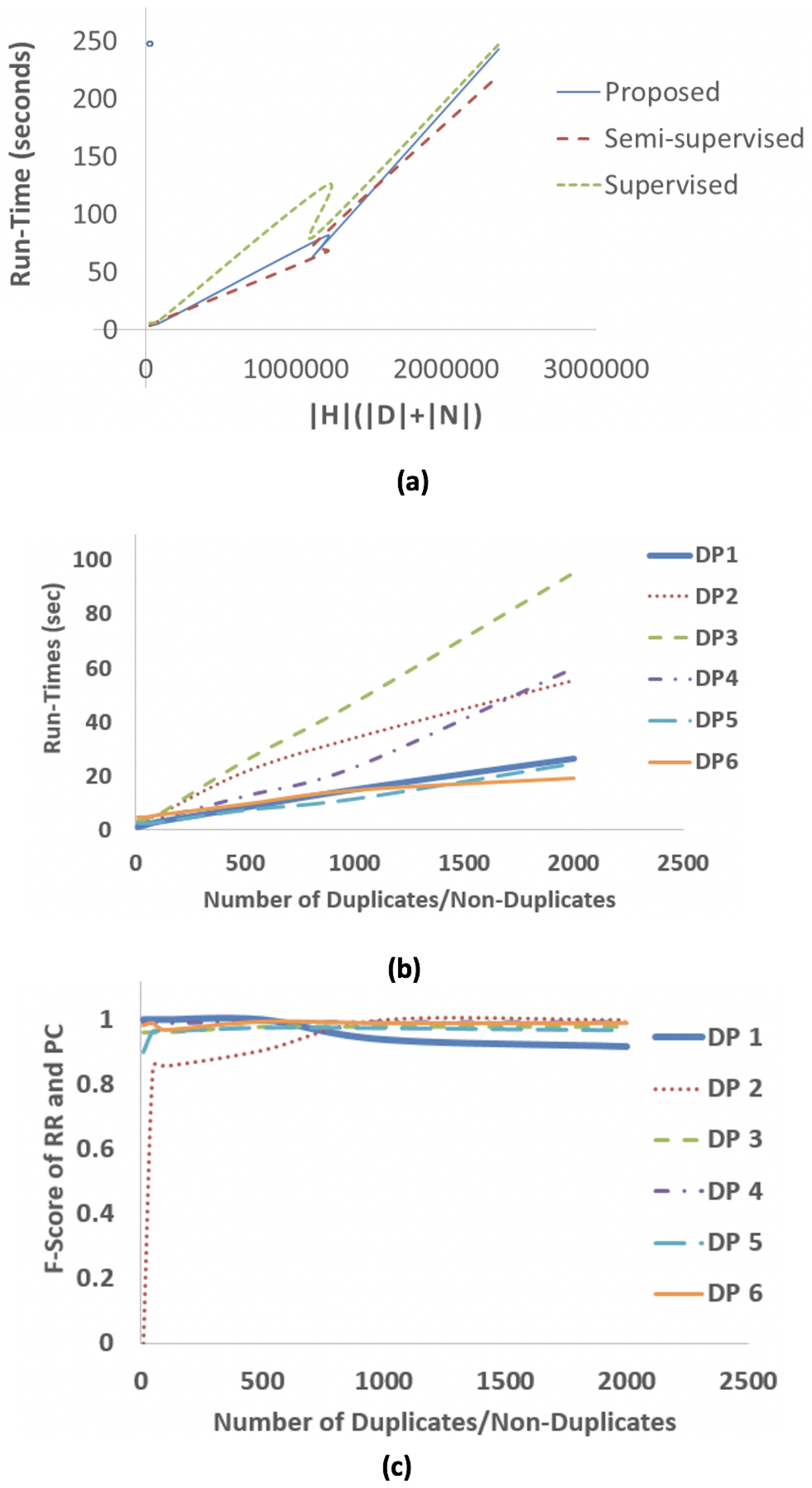
Theoretically, the run-time of Algorithm 1 was shown to be ${O\left(\right|H|}^k\left(\right|D|+\left|N\right|\left)\right)$; the run-times of other systems in Table 1 are similar. Empirically, this has never been demonstrated. For $k=1$, we plot the run-time data that were collected from Experiment 1 runs on DPs 1–6 (Figure 9a). The trend is fairly linear, with the supervised system slower for smaller inputs, but not larger inputs. The dependence on $\left|Q\right|$ shows why a schema matcher is necessary, since, in its absence, the simple exhaustive set is input (Section 5.3).

As further validation of the theoretical run-time, Figure 9b shows the linear dependence of the proposed system on $\left|D\right|$. Again, the trend is linear, but the slope (note that the slope is the hidden constant in the asymptotic notation) depends on the schema heterogeneities of the individual DPs. For example, DPs 2 and 3, the largest datasets in terms of fields (Table 3), do not scale as well as the others.

Figure 9c shows an important robustness result. We plot the PC-RR f-score ($\frac{2.RR.PC}{RR+PC}$) of the proposed system against $\left|D\right|$. The first observation is that, even for small $\left|D\right|$, performance is already high except on DP 2, which shows a steep increase when $\left|D\right|\approx 100$. On all cases, maximum performance is achieved at about $\left|D\right|\approx 700$ and the f-score curves flatten subsequently. This is qualitatively similar to the robustness of Dumas to small numbers of positive samples.

Figure 9c also shows that the proposed method is robust to overestimates of $\left|D\right|$. DP 1, for example, only has 100 true positives, but it continues to perform well at much higher $\left|D\right|$ (albeit with a slight dip at $\left|D\right|\approx 700$).

9. Discussion

Earlier, when discussing the preliminary experimental results evaluating Dumas (Section 7.2), we noted that an extended DNF-BSL can only integrate well into the pipeline if it is robust to noise from previous steps. Previous research has noted the overall robustness of DNF-BSLs. This led to the recent emergence of a homogeneous unsupervised system [7], which was adapted here as a semi-supervised baseline. Experiment 1 results showed that this robustness also carries over to extended DNF-BSLs. High overall performance shows that the pipeline can accommodate heterogeneity, a key goal of this paper.

Experiment 2 results demonstrate the advantage of having an expressive G, which is evidently more viable than increasing k. On DPs 1 and 5 (that the systems succeeded on), no statistically significant differences were observed, despite the run-time increasing by a factor of 16. We note that the largest (homogeneous) test cases on which $k=2$ schemes were previously evaluated were only about the order of DP 1 (in size). Even with less expressive G, only a few percentage point performance differences were observed (in PC and RR), with statistical significance not reported [4,7].

In order to confirm the role of G, we performed a follow-up experiment where we used the originally proposed G [4] on DPs 1 and 5, with both $k=1$ and $k=2$. We observed lower performance with $k=1$ compared to Table 4 results, while $k=2$ results were only at par with those results. The run-times with less expressive G were obviously lower (for corresponding k); however, $k=2$ run-times were higher (with less expressive G) than $k=1$ run-times with more expressive G. All of the differences just described were statistically significant (at the 95% level). This validates previous research findings, while also confirming our stated hypothesis regarding G.

The Experiment 3 results showed that a sophisticated schema matcher is not always necessary for the purpose of learning a blocking scheme. However, the importance of good schema matching goes beyond blocking and even ER. Schema matching is an important step in overall data integration [47]. On noisier datasets, a good n:m schema matcher could make all the difference in pipeline performance, but we leave it for future work to evaluate such a case.

The similar run-time trends that were shown by the various systems in Figure 9a also explain why, in Experiment 2, all the systems simultaneously succeeded or failed on a given DP. Even if we replace our DNF-BSL with an extended version from the literature, the exponential dependence on k remains. Figure 9a,b also empirically validate theoretical run-time calculations. Previous research on DNF-BSLs did not theoretically analyze (or empirically report) the algorithmic run-times and scalability explicitly [4,5,6,7].

Figure 9c demonstrates the encouraging qualitative result that only a few (noisy) samples are typically enough for adequate performance. Given enterprise quality requirements, as well as expense of domain expertise, high performance for low n and minimum parameter tuning is a practical necessity, for industrial deployment. Recall that we retained $\kappa$ at 0.9 for all experiments (after tuning on DP 1), while for the baselines, we had to conduct parameter sweeps for each separate experiment. When combined with the results in both Table 4 and Figure 9c, this shows that the system can be a potential use-case in industry. Combined with previous unsupervised results for the second ER step [1,2], such a use-case would apply to both relational and Semantic Web data as a fully unsupervised ER workflow, which has thus far remained elusive.

10. Conclusions and Future Work

In this paper, we presented a generic pipeline for learning DNF blocking schemes on heterogeneous dataset pairs. We proposed an unsupervised instantiation of the pipeline that relies on an existing instance-based schema matcher and learns blocking schemes while using only two parameters. We also showed a novel way of reconciling RDF-tabular heterogeneity by using the logical property table representation for building and populating a dynamic property schema for RDF datasets. Finally, we evaluated all the techniques on six test cases exhibiting three separate kinds of heterogeneity.

Future research will address further exploration of the property table representation for tabularly mining RDF data. Additionally, refining G (the set of GBPs) further is a promising, proven method of scalably improving BSL performance. We will also implement a fully unsupervised ER workflow that the proposed unsupervised DNF-BSL enables, and evaluate it in a similar fashion. Another important area of improvement is to devise better-performing self-training methods (see, for example, the work by [64]) rather than relying on the noisy examples that were produced by Dumas. Incorporating representation learning into the pipeline is clearly something that could add value and improve performance, but it is unclear whether representation learning is compatible with the set of GBPs. Investigating this further is also an issue for future research. Last, but not least, we also intend to expand the pipeline, so that it can learn a BSL on more than two structurally heterogeneous datasets (or what we referred to as a dataset pair in the experiments). In principle, the approach can be extended to accommodate multiple structurally heterogeneous datasets, but evaluating the approach on large collections of datasets (each of which may individually also be large) remains an open challenge.

References

1. Elmagarmid, A.K.; Ipeirotis, P.G.; Verykios, V.S. Duplicate record detection: A survey. IEEE Trans. Knowl. Data Eng. 2007, 19, 1–16. [Google Scholar] [CrossRef] [Green Version]
2. Ferraram, A.; Nikolov, A.; Scharffe, F. Data linking for the semantic web. Int. J. Semant. Web Inf. Syst. 2013, 7, 169. [Google Scholar]
3. Christen, P. A survey of indexing techniques for scalable record linkage and deduplication. IEEE Trans. Knowl. Data Eng. 2012, 24, 1537–1555. [Google Scholar] [CrossRef] [Green Version]
4. Bilenko, M.; Kamath, B.; Mooney, R.J. Adaptive blocking: Learning to scale up record linkage. In Proceedings of the Sixth International Conference on Data Mining (ICDM’06), Hong Kong, China, 18–22 December 2006; pp. 87–96. [Google Scholar]
5. Michelson, M.; Knoblock, C.A. Learning blocking schemes for record linkage. In Proceedings of the National Conference on Artificial Intelligence, Boston, MA, USA, 16–20 July 2006. [Google Scholar]
6. Cao, Y.; Chen, Z.; Zhu, J.; Yue, P.; Lin, C.Y.; Yu, Y. Leveraging unlabeled data to scale blocking for record linkage. In Proceedings of the International Joint Conference on Artificial Intelligence, Barcelona, Spain, 16–22 July 2011; p. 2211. [Google Scholar]
7. Kejriwal, M.; Miranker, D.P. An unsupervised algorithm for learning blocking schemes. In Proceedings of the Thirteenth International Conference on Data Mining (ICDM’13), Dallas, TX, USA, 7–10 December 2013. [Google Scholar]
8. Bizer, C.; Heath, T.; Berners-Lee, T. Linked data-the story so far. Int. J. Semant. Web Inf. Syst. 2009, 5, 1–22. [Google Scholar] [CrossRef] [Green Version]
9. Volz, J.; Bizer, C.; Gaedke, M.; Kobilarov, G. Discovering and maintaining links on the web of data. In The Semantic Web-ISWC 2009; Springer: New York, NY, USA, 2009; pp. 650–665. [Google Scholar]
10. Xu, D.; Ruan, C.; Korpeoglu, E.; Kumar, S.; Achan, K. Product knowledge graph embedding for e-commerce. In Proceedings of the 13th International Conference on Web Search and Data Mining, Houston, TX, USA, 3–7 February 2020; pp. 672–680. [Google Scholar]
11. Kejriwal, M.; Liu, Q.; Jacob, F.; Javed, F. A pipeline for extracting and deduplicating domain-specific knowledge bases. In Proceedings of the 2015 IEEE International Conference on Big Data (Big Data), Santa Clara, CA, USA, 29 October–1 November 2015; pp. 1144–1153. [Google Scholar]
12. Selvam, R.K.; Kejriwal, M. On using Product-Specific Schema. org from Web Data Commons: An Empirical Set of Best Practices. arXiv 2020, arXiv:2007.13829. [Google Scholar]
13. Singhal, A. Introducing the knowledge graph: Things, not strings. Off. Google Blog 2012, 5, 16. [Google Scholar]
14. Reese, J.T.; Unni, D.; Callahan, T.J.; Cappelletti, L.; Ravanmehr, V.; Carbon, S.; Shefchek, K.A.; Good, B.M.; Balhoff, J.P.; Fontana, T.; et al. KG-COVID-19: A framework to produce customized knowledge graphs for COVID-19 response. Patterns 2021, 2, 100155. [Google Scholar] [CrossRef]
15. Kejriwal, M. Knowledge Graphs and COVID-19: Opportunities, Challenges, and Implementation. Harv. Data Sci. Rev. 2020. [Google Scholar] [CrossRef]
16. Wilkinson, K.; Sayers, C.; Kuno, H.A.; Reynolds, D. Efficient RDF Storage and Retrieval in Jena2. In Proceedings of the 1st International Workshop on Semantic Web and Databases, Co-located with VLDB 2003, Berlin, Germany, 7–8 September 2003; pp. 131–150. [Google Scholar]
17. He, B.; Patel, M.; Zhang, Z.; Chang, K.C.C. Accessing the deep web. Commun. ACM 2007, 50, 94–101. [Google Scholar] [CrossRef]
18. Bilke, A.; Naumann, F. Schema matching using duplicates. In Proceedings of the 21st International Conference on Data Engineering, Tokoyo, Japan, 5–8 April 2005; pp. 69–80. [Google Scholar]
19. Benjelloun, O.; Garcia-Molina, H.; Menestrina, D.; Su, Q.; Whang, S.E.; Widom, J. Swoosh: A generic approach to entity resolution. Int. J. Very Large Data Bases 2009, 18, 255–276. [Google Scholar] [CrossRef] [Green Version]
20. Papadakis, G.; Skoutas, D.; Thanos, E.; Palpanas, T. Blocking and filtering techniques for entity resolution: A survey. ACM Comput. Surv. 2020, 53, 1–42. [Google Scholar] [CrossRef] [Green Version]
21. Kejriwal, M. Domain-Specific Knowledge Graph Construction; Springer: New York, NY, USA, 2019. [Google Scholar]
22. Nam, D.; Kejriwal, M. How Do Organizations Publish Semantic Markup? Three Case Studies Using Public Schema. org Crawls. Computer 2018, 51, 42–51. [Google Scholar] [CrossRef]
23. Noy, N.; Gao, Y.; Jain, A.; Narayanan, A.; Patterson, A.; Taylor, J. Industry-scale knowledge graphs: Lessons and challenges. Commun. ACM 2019, 62, 36–43. [Google Scholar] [CrossRef] [Green Version]
24. Christophides, V.; Efthymiou, V.; Stefanidis, K. Entity resolution in the web of data. Synth. Lect. Semant. Web 2015, 5, 1–122. [Google Scholar] [CrossRef] [Green Version]
25. Zhu, L.; Ghasemi-Gol, M.; Szekely, P.; Galstyan, A.; Knoblock, C.A. Unsupervised entity resolution on multi-type graphs. In Proceedings of the International Semantic Web Conference, Kobe, Japan, 17–21 October 2016; Springer: New York, NY, USA, 2016; pp. 649–667. [Google Scholar]
26. Kejriwal, M.; Miranker, D.P. An unsupervised instance matcher for schema-free RDF data. Web Semant. Sci. Serv. Agents World Wide Web 2015, 35, 102–123. [Google Scholar] [CrossRef]
27. Brown, T.B.; Mann, B.; Ryder, N.; Subbiah, M.; Kaplan, J.; Dhariwal, P.; Neelakantan, A.; Shyam, P.; Sastry, G.; Askell, A.; et al. Language models are few-shot learners. arXiv 2020, arXiv:2005.14165. [Google Scholar]
28. Xue, L.; Constant, N.; Roberts, A.; Kale, M.; Al-Rfou, R.; Siddhant, A.; Barua, A.; Raffel, C. mT5: A massively multilingual pre-trained text-to-text transformer. arXiv 2020, arXiv:2010.11934. [Google Scholar]
29. Devlin, J.; Chang, M.W.; Lee, K.; Toutanova, K. Bert: Pre-training of deep bidirectional transformers for language understanding. arXiv 2018, arXiv:1810.04805. [Google Scholar]
30. Wang, Q.; Mao, Z.; Wang, B.; Guo, L. Knowledge graph embedding: A survey of approaches and applications. IEEE Trans. Knowl. Data Eng. 2017, 29, 2724–2743. [Google Scholar] [CrossRef]
31. Kejriwal, M. Advanced topic: Knowledge graph completion. In Domain-Specific Knowledge Graph Construction; Springer: New York, NY, USA, 2019; pp. 59–74. [Google Scholar]
32. Kejriwal, M.; Szekely, P. Neural embeddings for populated geonames locations. In Proceedings of the International Semantic Web Conference, Vienna, Austria, 21–25 October 2017; Springer: New York, NY, USA, 2017; pp. 139–146. [Google Scholar]
33. Datar, M.; Immorlica, N.; Indyk, P.; Mirrokni, V.S. Locality-sensitive hashing scheme based on p-stable distributions. In Proceedings of the Twentieth Annual Symposium on Computational Geometry, Brooklyn, NY, USA, 9–11 June 2004; pp. 253–262. [Google Scholar]
34. Paulevé, L.; Jégou, H.; Amsaleg, L. Locality sensitive hashing: A comparison of hash function types and querying mechanisms. Pattern Recognit. Lett. 2010, 31, 1348–1358. [Google Scholar] [CrossRef] [Green Version]
35. Kim, H.s.; Lee, D. HARRA: Fast iterative hashed record linkage for large-scale data collections. In Proceedings of the 13th International Conference on Extending Database Technology, Lausanne, Switzerland, 22–26 March 2010; pp. 525–536. [Google Scholar]
36. Marçais, G.; DeBlasio, D.; Pandey, P.; Kingsford, C. Locality-sensitive hashing for the edit distance. Bioinformatics 2019, 35, i127–i135. [Google Scholar] [CrossRef] [Green Version]
37. Duan, S.; Fokoue, A.; Hassanzadeh, O.; Kementsietsidis, A.; Srinivas, K.; Ward, M.J. Instance-based matching of large ontologies using locality-sensitive hashing. In Proceedings of the International Semantic Web Conference, Boston, MA, USA, 11–15 November 2012; Springer: New York, NY, USA, 2012; pp. 49–64. [Google Scholar]
38. Ma, Y.; Tran, T.; Bicer, V. Typifier: Inferring the type semantics of structured data. In Proceedings of the 2013 IEEE 29th International Conference on Data Engineering (ICDE), Brisbane, Australia, 8–11 April 2013; pp. 206–217. [Google Scholar]
39. Shao, J.; Wang, Q.; Lin, Y. Skyblocking for entity resolution. Inf. Syst. 2019, 85, 30–43. [Google Scholar] [CrossRef] [Green Version]
40. Nascimento, D.C.; Pires, C.E.S.; Nóbrega, T.P. Configurable assembly of classification rules for enhancing entity resolution results. Inf. Process. Manag. 2020, 57, 102224. [Google Scholar] [CrossRef]
41. Uno, T.; Maegawa, H.; Nakahara, T.; Hamuro, Y.; Yoshinaka, R.; Tatsuta, M. Micro-clustering: Finding small clusters in large diversity. arXiv 2015, arXiv:1507.03067. [Google Scholar]
42. Kejriwal, M. Adaptive Candidate Generation for Scalable Edge-discovery Tasks on Data Graphs. arXiv 2016, arXiv:1605.00686. [Google Scholar]
43. Kejriwal, M.; Miranker, D.P. Sorted neighborhood for schema-free RDF data. In Proceedings of the European Semantic Web Conference, Portoroz, Slovenia, 31 May–4 June 2015; Springer: New York, NY, USA, 2015; pp. 217–229. [Google Scholar]
44. Kejriwal, M.; Miranker, D.P. A DNF blocking scheme learner for heterogeneous datasets. arXiv 2015, arXiv:1501.01694. [Google Scholar]
45. Kejriwal, M.; Miranker, D.P. Self-contained NoSQL Resources for Cross-Domain RDF. arXiv 2016, arXiv:1608.04437. [Google Scholar]
46. Kejriwal, M.; Miranker, D.P. On Linking Heterogeneous Dataset Collections. In Proceedings of the International Semantic Web Conference (Posters & Demos), Trentino, Italy, 19–23 October 2014; pp. 217–220. [Google Scholar]
47. Bellahsene, Z.; Bonifati, A.; Rahm, E. Schema Matching and Mapping; Springer: New York, NY, USA, 2011; Volume 20. [Google Scholar]
48. Gal, A. Why is schema matching tough and what can we do about it? ACM Sigmod Rec. 2006, 35, 2–5. [Google Scholar] [CrossRef] [Green Version]
49. Koumarelas, l.; Papenbrock, T.; Naumann, F. MDedup: Duplicate detection with matching dependencies. Proc. VLDB Endow. 2020, 13, 712–725. [Google Scholar] [CrossRef]
50. Caruccio, L.; Deufemia, V.; Polese, G. Mining relaxed functional dependencies from data. Data Min. Knowl. Discov. 2020, 34, 443–477. [Google Scholar] [CrossRef]
51. Sahoo, S.S.; Halb, W.; Hellmann, S.; Idehen, K.; Thibodeau Jr, T.; Auer, S.; Sequeda, J.; Ezzat, A. A Survey of Current Approaches for Mapping of Relational Databases to RDF; World Wide Web Consortium: Boston, MA, USA, 2009. [Google Scholar]
52. Sequeda, J.F.; Miranker, D.P. Ultrawrap: Sparql execution on relational data. J. Web Semant. 2013, 22, 19–39. [Google Scholar] [CrossRef] [Green Version]
53. Hernández, M.A.; Stolfo, S.J. The merge/purge problem for large databases. ACM Sigmod Rec. 1995, 24, 127–138. [Google Scholar] [CrossRef]
54. Kolb, L.; Thor, A.; Rahm, E. Multi-pass sorted neighborhood blocking with mapreduce. Comput. Sci. Res. Dev. 2012, 27, 45–63. [Google Scholar] [CrossRef]
55. Christen, P. Data Matching: Concepts and Techniques for Record Linkage, Entity Resolution, and Duplicate Detection; Springer: New York, NY, USA, 2012. [Google Scholar]
56. Chvatal, V. A greedy heuristic for the set-covering problem. Math. Oper. Res. 1979, 4, 233–235. [Google Scholar] [CrossRef]
57. Lee, Y.; Sayyadian, M.; Doan, A.; Rosenthal, A.S. eTuner: Tuning schema matching software using synthetic scenarios. Int. J. Very Large Data Bases 2007, 16, 97–122. [Google Scholar] [CrossRef]
58. Eiben, A.E.; Smit, S.K. Parameter tuning for configuring and analyzing evolutionary algorithms. Swarm Evol. Comput. 2011, 1, 19–31. [Google Scholar] [CrossRef] [Green Version]
59. Lovász, L.; Plummer, M.D. Matching Theory; Elsevier: Amsterdam, The Netherlands, 1986. [Google Scholar]
60. Raz, R.; Safra, S. A sub-constant error-probability low-degree test, and a sub-constant error-probability PCP characterization of NP. In Proceedings of the Twenty-Ninth Annual ACM Symposium on Theory of Computing, El Paso, TX, USA, 4–6 May 1997; pp. 475–484. [Google Scholar]
61. Peleg, D. Approximation Algorithms for the Label-Cover MAX and Red-Blue Set Cover Problems. In Algorithm Theory-SWAT 2000; Springer: New York, NY, USA, 2000; pp. 220–231. [Google Scholar]
62. Carr, R.D.; Doddi, S.; Konjevod, G.; Marathe, M.V. On the red-blue set cover problem. In Proceedings of the Eleventh Annual ACM-SIAM Symposium on Discrete Algorithms, San Francisco, CA, USA, 9–11 January 2000; pp. 345–353. [Google Scholar]
63. Tian, A.; Kejriwal, M.; Miranker, D.P. Schema matching over relations, attributes, and data values. In Proceedings of the 26th International Conference on Scientific and Statistical Database Management, Aalborg, Denmark, 30 June–2 July 2014. [Google Scholar]
64. Tkachenko, R.; Izonin, I. Model and principles for the implementation of neural-like structures based on geometric data transformations. In Proceedings of the International Conference on Computer Science, Engineering and Education Applications, Kiev, Ukraine, 18–20 January 2018; pp. 578–587. [Google Scholar]
Figure 1. A basic illustration of the two-step Entity Resolution (ER) workflow on two heterogeneous datasets (shown here as graphs with nodes and relations). Brute force comparisons would require quadratic time, even given a similarity function. The blocking step uses an inexpensive function (e.g., tokenizing and indexing on the last name, assuming the nodes represent people), called a blocking key, which is similar to traditional hashing, but (in the general case) can lead to overlapping blocks. The similarity function is now only applied to pairs of entities sharing blocks, leading to seven unique entity pairs. Based on the output of the similarity function, these pairs of entities will be determined to refer to the same underlying entity (or not).
Information 12 00134 g001
Figure 2. An instance of the Entity Resolution (ER) problem on two Resource Description Framework (RDF) knowledge graphs. In Semantic Web terminology, the ‘duplicate’ entities between the two graphs would need to be interlinked using a special property called owl:sameAs.
Information 12 00134 g002
Figure 3. Three example datasets exhibiting various kinds of heterogeneity. Dataset 1 is a knowledge graph (KG) that could be represented using RDF (for example), while the other two datasets form a pair of structurally heterogeneous tables.
Information 12 00134 g003
Figure 4. (a) shows a generic pipeline for learning a DNF blocking scheme on heterogeneous datasets, with (b) showing an unsupervised instantiation.
Information 12 00134 g004
Figure 5. Property table representation of Dataset 1 in Figure 3.
Information 12 00134 g005
Figure 6. An example showing how H c is formed.
Information 12 00134 g006
Figure 7. Step 1 of Algorithm 1, assuming the information in Figure 6.
Information 12 00134 g007
Figure 8. Dumas duplicates-generation results, for k { 1 , 2 50,000}.
Information 12 00134 g008
Figure 9. Experiment 4 results. (a) plots run-time trends of all three systems against the theoretical formula, while (b,c), respectively, plot run-times and f-scores of the proposed system against sample sizes.
Information 12 00134 g009