Short-Term Load Forecasting Based on the Transformer Model

Abstract

From the perspective of energy providers, accurate short-term load forecasting plays a significant role in the energy generation plan, efficient energy distribution process and electricity price strategy optimisation. However, it is hard to achieve a satisfactory result because the historical data is irregular, non-smooth, non-linear and noisy. To handle these challenges, in this work, we introduce a novel model based on the Transformer network to provide an accurate day-ahead load forecasting service. Our model contains a similar day selection approach involving the LightGBM and k-means algorithms. Compared to the traditional RNN-based model, our proposed model can avoid falling into the local minimum and outperforming the global search. To evaluate the performance of our proposed model, we set up a series of simulation experiments based on the energy consumption data in Australia. The performance of our model has an average MAPE (mean absolute percentage error) of 1.13, where RNN is 4.18, and LSTM is 1.93.

1. Introduction

With the advancement of the smart grid and the growing demand for economically efficient electricity scheduling, short term load forecasting (STLF) has attracted more attention in both industry and academia. From the perspective of energy providers, the accuracy of short-term load forecasting (STLF) plays a significant role in energy generation planning, efficient energy distribution processing and electricity price strategy optimisation. The concept of load forecasting was proposed by [1] in 1966. In [1], the relationship between the summer weather and peak load of utility systems was discussed by examining historical data.

According to the prediction horizon and purpose, load forecasting problems can be categorised into four types: very short-term load forecasting, short-term load forecasting, medium-term load forecasting, long-term load forecasting. The very short-term load forecasting refers to prediction time ranging from a few minutes to hours, aiming to help utility make decisions in real-time operation. Short-term load forecasting refers to load prediction one day ahead or one week ahead, aiming to increase energy schedule efficiency. Medium-term load forecasting represents the prediction approach with a time horizon range from one month to one year. According to [2], the goal of the medium terms load forecasting is make an effective operational plan. Long-term load forecasting is usually used for considering future financial plans and energy infrastructure dilation. The forecasting time range of long-term load prediction is more than one year. In this paper, we mainly put focus on short term load forecasting. To emphasise the importance of forecasting model accuracy, In [3], the author proposed that more than 10,000 MW energy will be saved if the mean absolute percentage error decrease 1%. However, a series of external time-variant factors can affect the power demand, such as weather, seasonal characteristics, temperature, etc. These factors make the problem more complex and arduous.

In the past decades, time-series forecasting has become an active issue and prompted a significant amount of research. The mainstream approaches of STLF can be classified into traditional statistical techniques and artificial-based approaches. Conventional statistical methods often involve double seasonal Holt-Winters exponential smoothing [4], linear regression, auto-regressive integrated moving average [5] etc. However, these approaches do not always work satisfactorily as these models adopt linear functions to process the relationship between the actual and forecasted data. However, the STLF issue can be concluded as a nonlinear, non-stationary time series forecasting problem. The artificial-based approaches are nonlinear forecasting models that employ nonlinear functions to predict load demand. Compared to the traditional linear model, nonlinear models are more suitable to solve complex load forecasting issues. The artificial-based approaches can be categorised into support vector machine (SVM) [6], fuzzy logistic methods [7], artificial neural network [8] etc. The artificial neural network mechanism produces reasonable results by mimicking the human brain to learn from past patterns and experiences. Compared with traditional statistical approaches, the artificial neural network method is a data-driven approach that has outstanding learning ability and adaptive function. This characteristic is very suitable for the time series forecasting problem. Recurrent neural network is a typical deep learning approaches which can capture sequence information in the time-series data and sharing parameters across different time lengths.

Nevertheless, the accuracy of recurrent neural network models is affected by the vanishing gradient and exploding issues, common challenges in various neural network models. To mitigate the impact of these two features, special architecture of the recurrent neural network, named long short term memory (LSTM), has been proposed. Compared to the standard recurrent neural network, there are two transfer states in LSTM. It only remembers the essential information, which leads to outstanding performance over long sequences of input.

Due to these features and challenges, it is essential to develop a more effective model. Our contributions are shown below. We implement a short term load forecasting model based on the transformer algorithm. Meanwhile, We proposed a novel similar day selection approach that combines LightGBM and K-means algorithm to calculate the importance of each feature and select the similar days from historical time series data. To validate the performance of our proposed model, we adopt the New South Wales load forecasting as a case study and implement our proposed model. The experiment result proves that, compared to other existing state-of-the-art approaches, our model shows outstanding performance.

The remainder of this paper is organised as follows. Section 2 briefly introduced the mainstream approaches for the short term load forecasting problem. Section 3 contains the introduction of the proposed STLF problem and the details of our proposed model. In Section 4, we compare our proposed model’s forecasting performance with other mainstream approaches through various evaluation metrics and provide a comprehensive experiment analyse. Section 5 elaborates the conclusion and analyse the future development directions.

2. Literature Review

In the past few decades, various prediction models have been proposed to tackle the challenge of STLF and satisfy the accuracy requirement. Based on the model’s mechanism, the mainstream approaches of STLF can be classified into statistical models and machine learning models. The following sections will briefly introduce each method’s features and discuss their merits and demerits.

Compared to other complex forecasting approaches, regression models are straightforward and easy to interpret. Based on the above reasons, numerous attempts have been made to develop the regression-based model. In [9], a multiple regression model was applied to solve the STLF problem in a trim scale level (a campus in London). The author developed a multiple regression model and a genetic model separately. Both of them have five essential independent factors (ambient temperature, solar radiation, relative humidity, wind speed and weekday index). The experiment result showed that the genetic programming model performs better than the multiple regression model concerning the total absolute error. Nevertheless, the stability and generalisation ability of this model still needs to be improved. In [10], the author employed the fuzzy linear regression model, which outperforms linear based forecast models. In [10], the experiment result revealed that the model performs outstandingly, with an average maximum percentage error is 3.5%. In [4], a model based on the Holt-Winters exponential smoothing methods was proposed to analyse the seasonal time series data. However, this approach is only applicable for the time series issue that exhibits seasonal behaviour. The authors in [11] presented an investigation based on the multiple linear regression method to solve the STLF issue. The author summarised that the multiple linear regression method for STLF is easy to develop, with the accuracy of historical data being a limitation of this model. The author also pointed out that the model’s accuracy depends on the fitting degree between the regression function and experiment data. Ref. [11] introduced a Multi parameter regression method to forecast the load data of the coming hours. The author indicated that the load demand trend depended on a few parameters. In conclusion, the regression-based model’s advantages are simple computation principle and structure, outstanding performance on extrapolation, and satisfying performance for a situation that has not occurred before. However, the general drawbacks of the regression-based model are that historical data is large, the model cannot describe each factor in detail, and the model is difficult to initialise.

The work in [12] introduced and tested the performance of several fuzzy time series (FTS) algorithms for the STLF problem. The author concluded that the mathematical and statistic knowledge requirement of the FTS algorithm is more accessible to fulfil than other mainstream prediction approaches. Furthermore, [12] pointed out that FTS shows an outstanding forecasting ability in very short-term load forecasting problems. The author assumed this might be caused by various seasonal factors, such as peak demands, unusual demands, etc. From a practical application perspective, the standard fuzzy logic-based model cannot fulfil the accuracy requirement of STLF. Compared to the classic fuzzy models, which employed heuristics defined membership functions, ref. [13] proposed a novel hybrid bio-inspired algorithm based on particle swarm optimisation algorithm and fuzzy inference method to enhance the model’s forecasting capability. Adika [13] discussed the limitations of the traditional conventional fizzy logic system in the complex problem. The results showed that the proposed hybrid model achieved higher accuracy than the classic fuzzy inference model.

In terms of the machine learning approach. Support vector machine is an algorithm that assigns labels to experiment objects through learning by sample [14]. Since the algorithm has advantages such as strong generalisation ability, global optimisation and fast computation speed, numerous attempts have been made to develop a support vector machine-based model [6,15,16]. In [6], the author stated that the SVM algorithm can reflect the non-linear relationship between influence factors and electricity load sequence. The experiment results prove that the SVM algorithm performs better when the problem is small-scale, sample and nonlinear. In [15], the author stated that compared to the backpropagation neural network, SVM performed better in prediction speed and accuracy. A comprehensive analysis and comparison of the forecasting ability of SVM and Auto-Regressive Integrated Moving Average(ARIMA) were presented in [16]. The experiment results proved that SVM achieves better performance for nonlinear patterns. However, the author also indicated that the ARIMA based approach is more appropriate for dealing with the approximation of linear type of load. In conclusion, most SVM-based models have poor performance when dealing with fuzzy phenomena.

The neural network-based approach has become the desired predictive approach and reveals a predominance performance compared to other mainstream approaches. In [17], the artificial neural network was first time used for the STLF. A back-propagation neural network-based model focusing on a complicated STLF problem with dynamic and non-linear factors was introduced in [17]. The author reduced the model’s training time by combining back-propagation with a rough set and filtering noise data. The results showed the superiority of the proposed model. Furthermore, [18] provided a comprehensive analysis of the relationship between weather conditions and load demand. The author in [18] proposed a prediction model based on a back-propagation neural network. A shallow neural network-based model was proposed in [12]. The author employed an artificial neural network approach to obtain the relationship between past and future data. Ref. [19] developed a feed-forward neural network for forecasting weather-sensitive loads. Compared to the traditional artificial neural network, the proposed model in this study is not fully connected. On the other hand, the model can receive a series of related factors: load time series, weather information and day type information. The proposed model displayed better prediction capability than the auto-regressive integrated moving average model on the same task with this extra information. However, in recent years, numerous attempts have been made to develop a modified feed-forward neural network-based STLF model. A deep residual network-based model was introduced in [20]. The author increased the model’s generalisation capability by adopting a two-stage ensemble strategy. The performance of the proposed model was validated by implementing it in various public data sets. The results showed that the proposed model significantly enhanced the prediction accuracy index compared to traditional regression models. With the north American utility dataset, the model’s MAPE can achieve 1.69.

Convolutional neural networks (CNN) were initially designed for data restructured in a grid-like topology. In most cases, the form of input data for CNN is two-or three-dimensional. However, one-dimensional data, such as time series load sequence, is also suitable for CNN. Furthermore, the CNN-based model excels in tackling the real-time problem because its properties of local connectivity and parameter sharing can reduce training time and increase training efficiency. The CNN has been widely applied to various application scenarios, such as computer vision tasks, voice recognition, audio generation, etc. However, only a few attempts have been made to develop a CNN -based model to solve the STLF problem. The work [21] presented a temporal convolutional network (TCN)-based deep learning model on solving the STLF problem. TCN is a particular architecture of CNN that combines the advantages of convolutional neural networks and recurrent neural networks. A comprehensive experiment was conducted in [21], the results of which prove that the proposed TCN based model outperforms the standard recurrent network-based model in prediction accuracy on the same task. Ref. [22] proposed a CNN- based model for the STLF problem at a single-building level. A comprehensive comparison of prediction accuracy among CNN, long short-term memory, ANN and SVM are provided in [22]. The experiment results showed that the RMSE of CNN based model is 0.677 which is close to LSTM based model.

In the past decades, due to the recurrent neural network being capable of exploiting the dependencies in the load data sequence, a significant number of attempts have been made to adapt it to achieve higher forecasting accuracy. The authors in [23] developed a prediction model based on the elmann recurrent neural network. In [23], the author implemented the model in a simulation environment and compared the prediction results between the weather-sensitive model and the non-weather-sensitive model. The author indicated that the proposed model is suitable for multi-input data. Another study The work in [24] also adopted the Elman recurrent neural network-based model to predict a suburban electricity load demand. In [24], the author included some extra factors, such as temperature, humidity and day type information, to increase the model’s prediction capability. Besides these relative factors, the author proposed a new index named ad hoc. The proposed new index can reflect the influence of the air-conditioner usage profile to load demand. In [25], a framework was designed for individual-level residential building load forecasting based on the LSTM algorithm. The framework was validated on a public access data-set, including actual resident load data, and showed outstanding performance. However, in [25], the prediction object is the individual level. The authors in [26] developed an LSTM based model designed for the area load prediction. The experiment revealed that the LSTM-based model outperforms other traditional prediction approaches when dealing with complex univariate sequence data. The authors in [27] made an exhaustive comparison of electricity load prediction accuracy between gradient boosting tree-based model, support vector regression-based model and LSTM based model. The MAPE of the proposed model is 8.935%, where support vector regression and gradient boosting tree are 10.391% and 9.512%, respectively. Ref. [28] stated that multivariate input data is capable of enhancing the LSTM model’s prediction capability. In [28], a genetic algorithm was adopted to obtain suitable time lags and the number of layers for the proposed LSTM-RNN-based model. The results proved the author’s perspective and shows that the LSTM-RNN-based model has the highest accuracy compared to other contemporary machine learning approaches. [29] employed gated recurrent unit neural networks. The author preprocessed the load data to avoid interference caused by the customer use characteristic. The experiment result shows that the average MAPE of the proposed model is no more than 11%, and the author indicated that the proposed model has faster convergence compared to LSTM. Compared to the standard RNN-based model, the LSTM-based model can reduce the effect of gradient disappearance. However, both of them were unable to generate output with arbitrary length and hard to parallelise on GPUs [30].

Furthermore, some studies also focus on the hybrid-based model, which aims to combine both sub-model advantages. A novel hybrid model was presented in [31], named parallel_CNN_RNN. In [31], CNN is employed to extract features of the input data, with RNN in charge of modelling the implicit dynamics data. The forecasting time horizon of the proposed model is day-ahead, and the results showed that the average MAPE was 1.405. The work in [32] adopted a similar approach, employing CNN to extract the trend and LSTM to obtain the relationship among time steps. The results revealed that the average MAPE was 0.0396, which outperforms other baseline models. Furthermore, [32] stated that the proposed model was more stable as compared to other standard deep learning approaches. With the LSTM-based model being widely implemented to resolve short-term load forecasting problems, a novel approach named sequence to sequence (seq2seq) gained research attention. This architecture’s original intention was to solve RNN’s limitation of generating output sequences with arbitrary length. In [33], an LSTM-based seq2seq model was proposed to forecast the electrical load, and the results proved the proposed model’s superiority as compared to the standard LSTM model.

3. Materials and Methodology

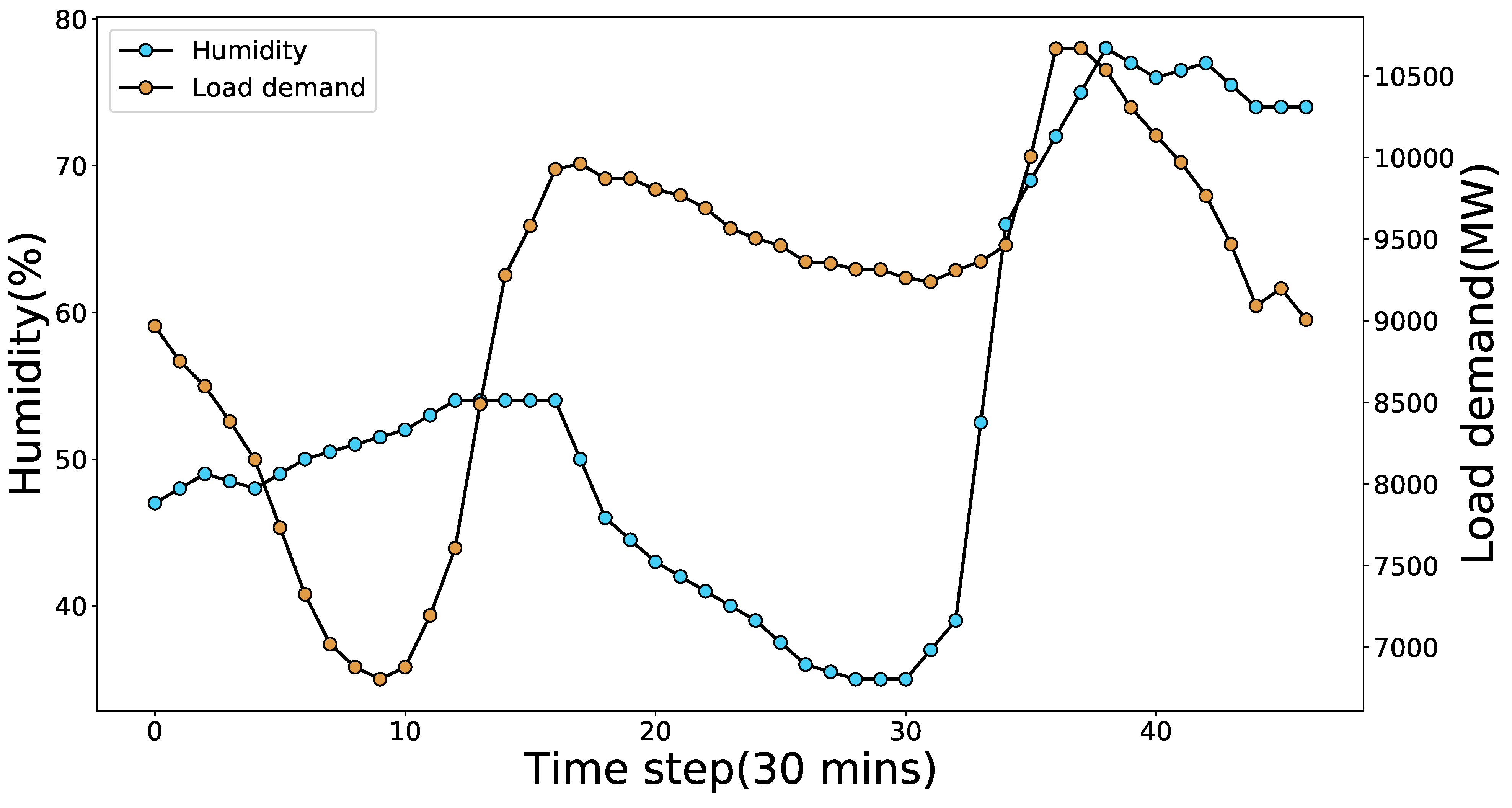
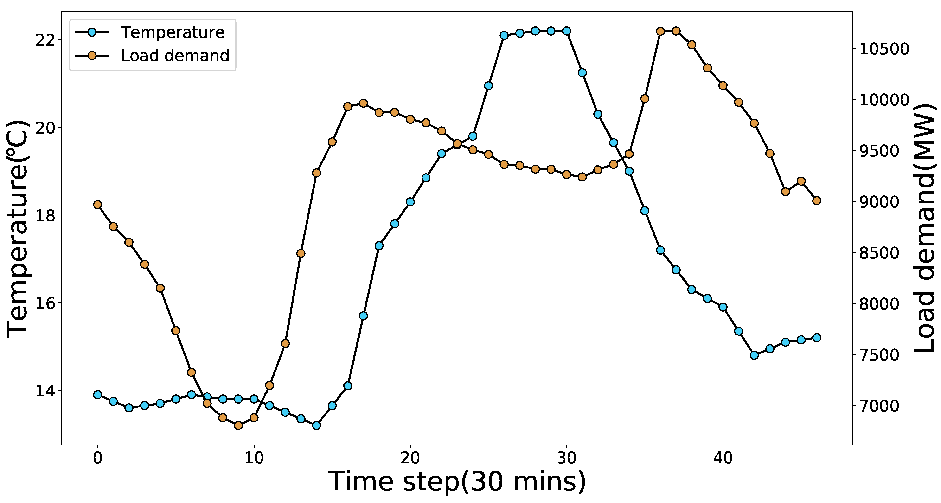
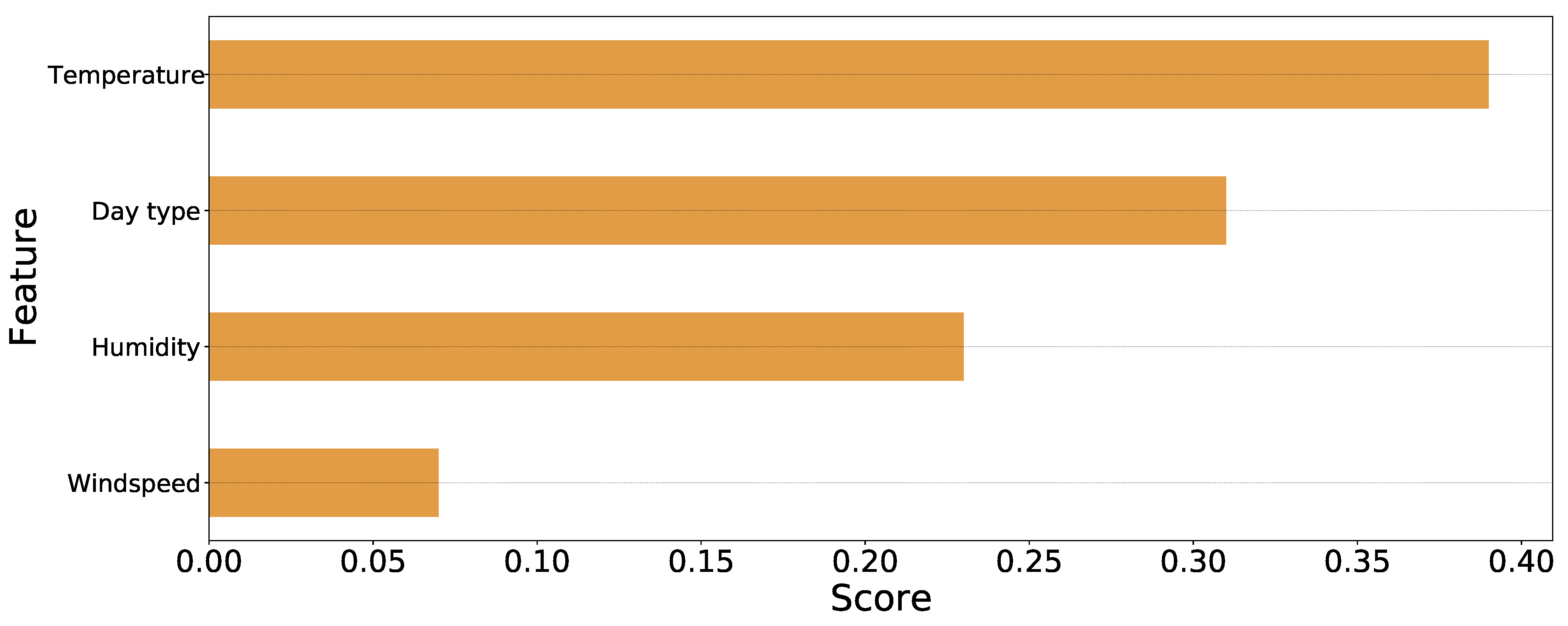
3.1. Data Collection

In this experiment, the dataset we adopted contains the electrical consumption profile in New South Wales from 1 January 2006 to 31 December 2010, which was obtained from the Australian Energy Market Operator. During this period, the load demand data was sampled every 30 min, which means 48 sampling points per day, 336 sampling points per week and 87,648 sampling points in total. Furthermore, This dataset also covers related factors, such as temperature, humidity and electricity price. The training set in our experiment includes 78,883 observations which represents the time period from 1 January 2006 T00:00 to 4 July 2010 T11:00. The test set contains 8765 observations from the period 4 July 2010 T11:30 to 31 December 2010 T23:30.

The following figures show the electricity consumption variation pattern from the perspective of different time scales. As we can see, day type is one of the key factors which affected the load demand. Figure 1 shows the variation of load demand within the time range of one week. The first point in Figure 1 represents the average value of load demand on each Monday midnight from 2006 to 2010. From the perspective of average value, the peak of load demands on the weekday are always higher than the weekend.

As mentioned before, the most relative factor affecting electricity consumption is weather. Figure 2 and Figure 3 represent the variation trend of humidity and temperature separately. In accordance with the analyse of the electricity usage data, we observed that season also affects the relationship between temperature and load demand. For instance, in winter, the load demand increases when the temperature decreases. However, this relationship is exactly the opposite in the summer. The reason for this phenomenon may be caused by the usages of air-conditional and residents’ behaviour profile.

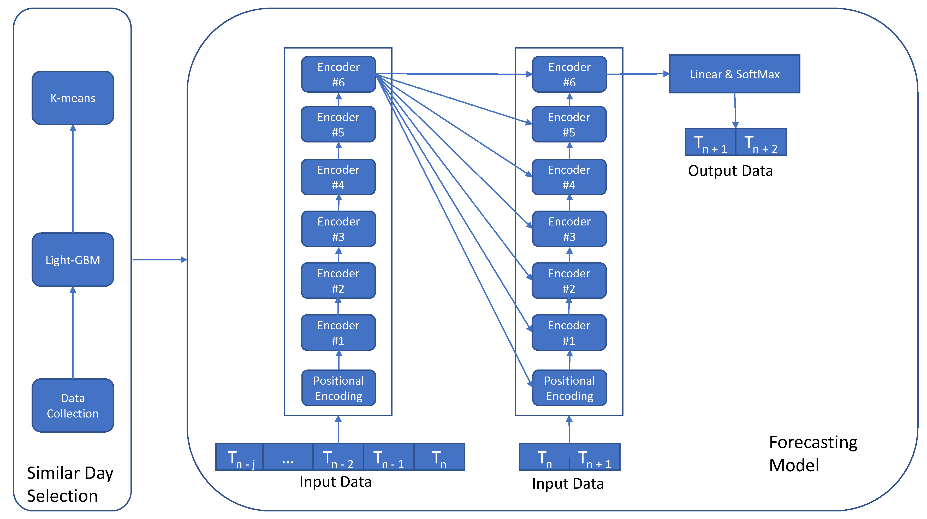
3.2. Problem Description and Model Overview

This section will present the details of the problem and briefly introduce our proposed forecasting model. The STLF task can be treated as a supervised machine learning problem. The input of our model is time-series data which consists of M days electricity load data points. With these input data points, the model needs to implement a multi-step ahead prediction. The format of the given data is $T_{n-j}, \dots , T_{n-2}, T_{n-1}, T_n$, and the output’s format is $T_{n+1}, \dots , T_{n+i}$.

Our forecasting system consists of two main components: Similar day selection and transformer-based forecasting model. As we mentioned before, to avoid slow convergence speed and poor prediction accuracy, we adopt similar day load data as the input data. We select similar days by clustering the entire historical data based on the feature data. K-means is one of the best-known clustering algorithms and has been used in a variety of studies. However, sometimes the performance of k-means will be affected by some unimportant factors. So we need to assign a unique weight value for each feature to avoid the dimensionality curse. In this case, we employed LightGBM to obtain the importance of an individual feature. The proposed forecasting model follows the original transformer architecture, which consists of encoder and decoder layers. Figure 4 illustrates the architecture of the entire system. Furthermore, we will introduce more details in the following sections.

3.3. Similar Day Selection

To enhance the model’s prediction capability, many previous studies adopted various relative factors, such as temperature, humidity, etc, to train the forecasting model. However, these exogenous features may also bring about a series of issues, such as slow convergence speed, forecasting accuracy decreased etc. To reduce the effect of the exogenous factors, we select the similar day’s load data as input instead of the previous day. Similar day selection approach is conventionally done by aggregating the data based on the extra relative factors and placing similar observations into the same cluster.

Traditional cluster algorithm calculates the distance between neighbours by measuring all factors equally. However, a series of irrelevant factors may affect the calculation result and the performance of the clustering algorithm. To overcome this shortage, we need to assign a weight to each factor, so the high relative feature is able to have more impact on the distance result rather than other irrelevant features. We employed a novel boosting decision tree algorithm named light gradient boosting machine (LightGBM) to calculate the weight parameter and k-means cluster algorithm to deal with the similar day selection.

3.3.1. LightGBM

LightGBM is an efficient, low memory footprint and high-accuracy gradient boosting framework proposed by [34] in 2017. LightGBM is a particular type of gradient boosting decision tree widely used for tackling tasks such as regression, classification and ranking, etc. The basic principle of gradient boosting decision tree is reducing the loss function by adopting a one-time iterative variable to enhance the weak classifiers during each iteration. In LightGBM, a boosted tree will be constructed, which is used to score each feature. The more times one feature is used, the higher score it gets. These feature scores represent the importance of the corresponding feature, and a higher score means that the feature is more relevant. To calculate each feature’s importance, LightGBM employs three columns: gain, cover and frequency. Gain refers to the total number of the feature’s splits. Cover pertains to the number of samples relative to this feature. Frequency indicates the times that the feature is used in the split process. In our experiment, we employed the gain-based approach to evaluate the importance score of each factor.

The decision tree in LightGBM is a binary tree structure that outputs qualified and not-eligible. The leaf-wise strategy of the decision tree in LightGBM is ’best first’, which means the node with max delta loss will be chosen to grow. However, for small-scale size data, this strategy may lead to the overfitting phenomenon. So, we set a parameter to restrict the max depth of the decision tree.

To obtain the importance of an individual feature, we replace the individual feature with random noise data and observe the final prediction result’s influence. With this approach, we can analyse the contribution of each individual feature to the final result. As mentioned before, the dataset includes various types of relative factors: temperature, humidity, wind speed and day type, which can be used to input the LightGBM. The result is shown in the below figure. Based on Figure 5, we can found that temperature is the most relative factor to the electric load compare to other factors. Furthermore, the load demand is also sensitive to the day type. However, wind speed only has a weak contribution to the final prediction result. In the next section, these weight parameters will be treated as prior knowledge for implementing the clustering algorithm.

3.3.2. k-Means

k-means is a popular clustering algorithm that was firstly proposed by [35] in 1967. Compared to other clustering algorithms, the mechanism of k-means is uncomplicated and simple to implement. The principle of the k-means algorithm involves clustering the entire dataset into various clusters base on the distance. The goal of the k-means algorithm is make the distance between each cluster centre as large as possible. The formula in Equation (1) represents the cluster set. In Equation (1), $C_k$ means the $k_{t}h$ cluster. Furthermore, the objective function of k-means algorithm is to minimise the square error $SE$, which can be formulated as Equation (2), where ${\beta }_t$ represents the mean vector of cluster $C_t$. In Equation (2), d represents the sample in the cluster $C_t$. Furthermore, ${\beta }_t$ can be formulated as Equation (3). The distance between the two samples can be calculated through Equation (4).

$$C=[C_1,C_2,C_3,\dots ,C_j]$$

(1)

$$SE=\sum _{t=1}^j\sum _{d\in C_i}{∥d-{\beta }_t∥}_2^2$$

(2)

$${\beta }_t=\frac{1}{\left|C_t\right|}\sum _{d\in C_t}d$$

(3)

$$Distance(d_i,N_i)=\sqrt{p_1{(d_{i1}-N_{i1})}^2+\dots p_n{(d_{in}-N_{in})}^2}$$

(4)

The following pseudo-code Algorithm 1 shows the basic workflow of k-means algorithm in our experiment. The output of the k-means algorithm is a repository that consists of m clusters. Firstly, we need to confirm the number of clusters, maximum iteration times T. Then, we need to confirm each cluster’s centre point. In this case, we assume the prediction as the first cluster centre. After all of the cluster centres have been confirmed, we need to re-traverse the entire dataset and assign each sample to the corresponding cluster. Then, the model will output the final cluster set. Equation (4) represents the distance calculation formulation in our algorithm. The weight parameters we obtain in the last section will play a critical role in this formula.

Algorithm 1. k-means Clustering

input: Dataset: $D=d_1, d_2, d_3, \dots , d_n$, cluster number: K, maximum iteration $T_{max}$,             The weight parameter set: $P=p_1, p_2, \dots , p_n$

output: Cluster set: $C=c_1, c_2, c_3, \dots , c_m$

Normalise the data set;

Select the forecasting day as the first cluster centre $N_1$;

$dis{t}_{max}=minvalue;$

$dis{t}_{min}=maxvalue;$

$N_{temp}=null;$

$E_{temp}=null;$

$k=1;$

return C;

In conclusion, The principle of similar day selection is to obtain the individual weights for each feature and make a cluster for the dataset based on the attribute weights. Compared to the standard k-means algorithm, our proposed hybrid approach is more effective.

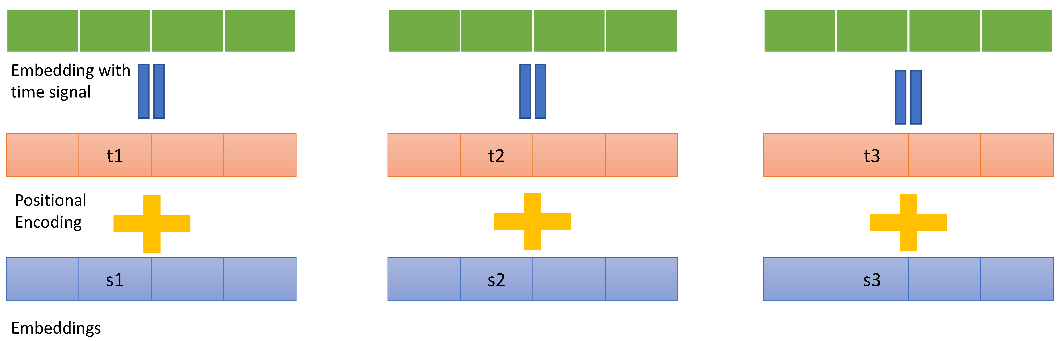
3.4. Forecasting Model

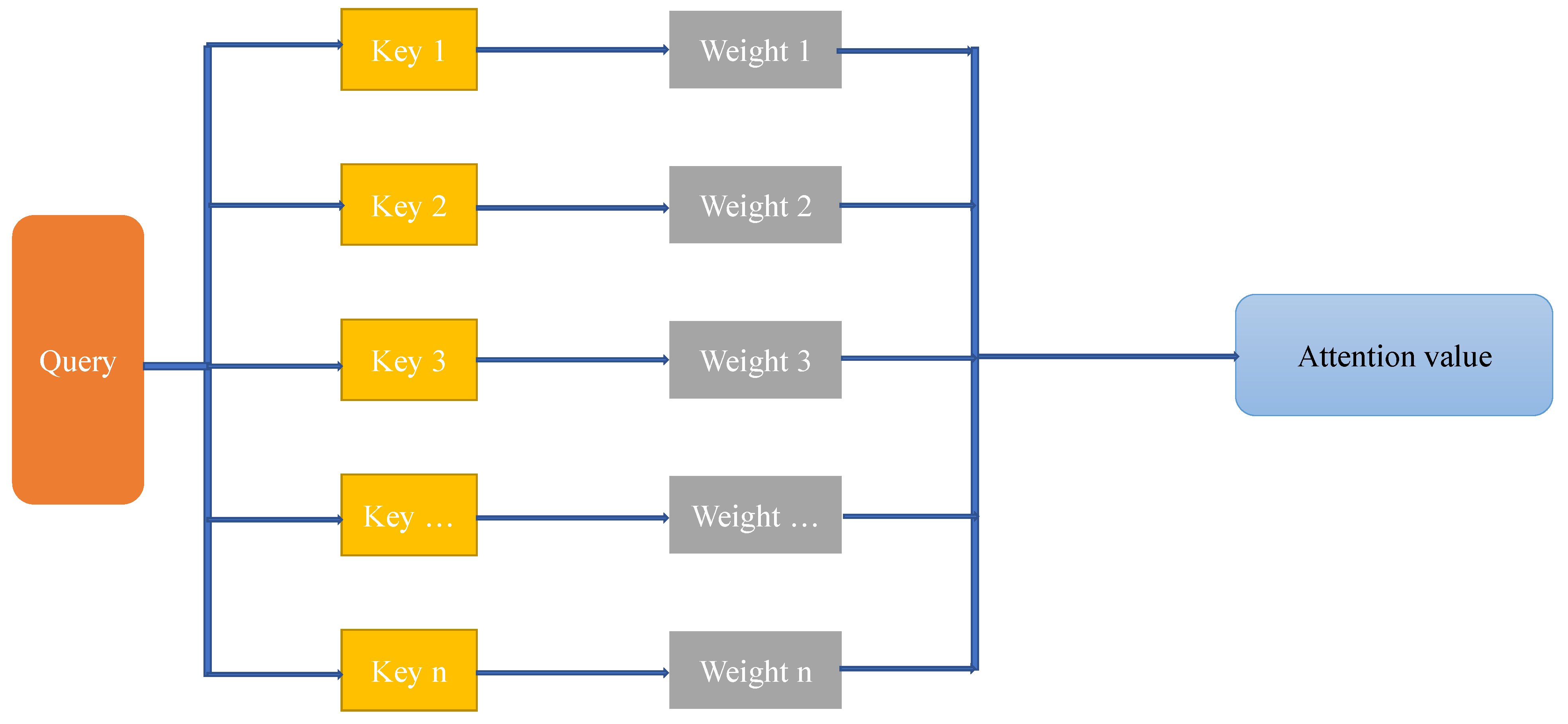
3.4.1. Attention Mechanism

In 2014, the Google research group proposed a novel RNN-based model named Attention, which can extract information from the image through processing specific regions at high resolution [36]. However, this model’s original intention was to tackle computer vision issues, such as image classification and natural language processing problems. A series of hybrid models combining the Attention mechanism and RNN-based network show outstanding performance on the time series forecasting problem. In 2017, the Google research lab presented a new simple model, named Transformer, which was based solely on Attention mechanisms [37]. The detail of the attention mechanisms and our proposed forecasting model will be introduced in the following sections.

The idea of the attention mechanism was inspired by the human visual attention mechanism. For instance, when we perceive visually, instead of putting the focus on the entire scene, we usually pay attention to a specific part based on our needs. If we found that the part we want to observe always exists in this scene, we will learn it, and the next time we face a similar scene, this part will attract our attention. The following figure illustrates the essence of the Attention mechanism.

We assume that our data source consists of a series of elements that can be represented as “$key,value$”. In Figure 6, Query is a query vector that is related to our target data. As we can see, the whole calculation process of attention can be divided into three stages. First, we need to compute the similarity score between the query vector and key vector according to Equation (5). After that, the score will be converted to weights by Equation (6). In the meanwhile, we need to normalised the weight set and sort it in probability distribution. According to [36], the sum of the entire element weight set equals to one. To emphasise the importance of some specific elements, [36] proposed employing (6) to make these selected elements more prominent. Finally, we perform a weighted summation of all the coefficients to compute the attention value, which can be formulated as Equation (7). As mentioned before, the core of the attention mechanism is computing the relative weight between encoder and decoder.

$$Simi(Queryvector,ke{y}_i)=\frac{Queryvector·ke{y}_i}{∥Queryvector∥·∥ke{y}_i∥}$$

(5)

$$w_i=Softmax\left(Sim{i}_i\right)=\frac{e^{Sim{i}_i}}{su{m}_{n=1}^N{e}^{Sim{i}_n}}fori=1,\dots ,N$$

(6)

$$Attentionscore(Query,Element(Key,Value))=\sum _{i=1}^N{w}_i·Valu{e}_i$$

(7)

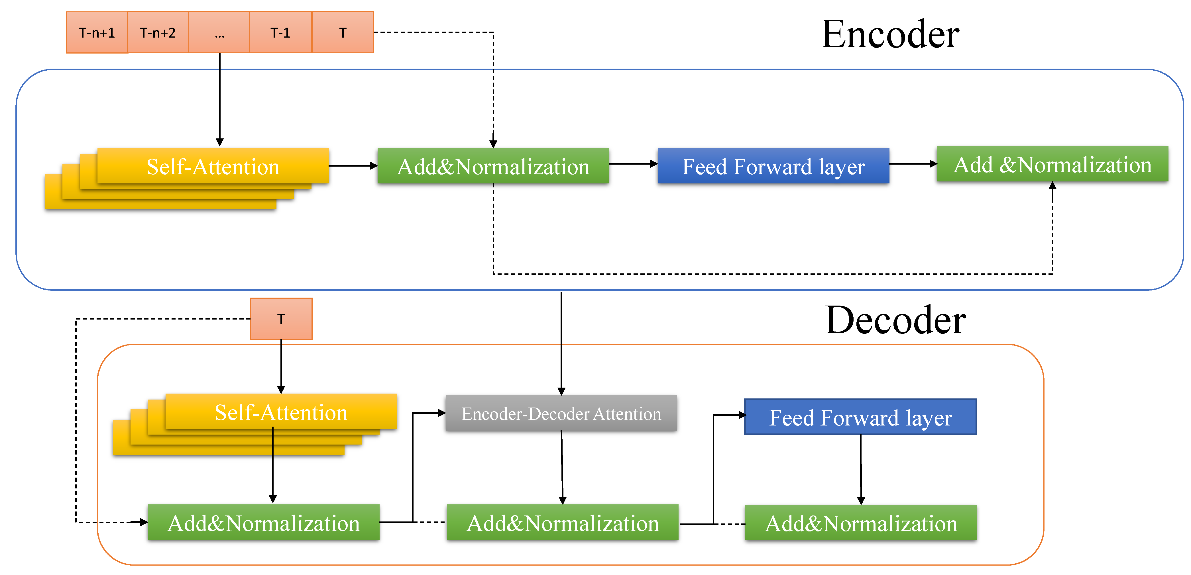
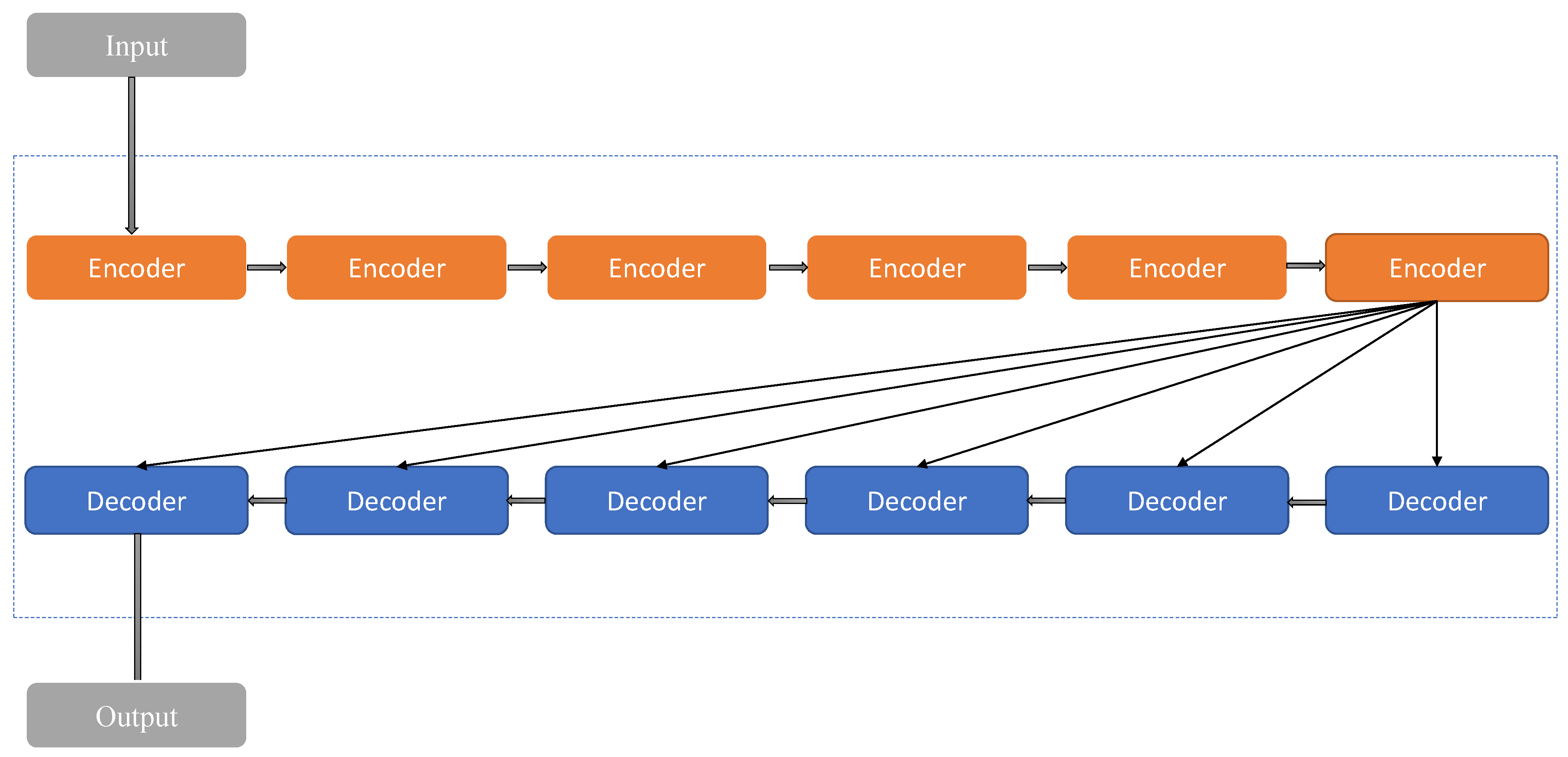
3.4.2. Transformer-Based Model

The transformer model, which is the first transduction model based solely on attention mechanisms, has better parallel capability than the LSTM algorithm. The core of the transformer model is an encoder-decoder architecture, which is illustrated in the following Figure 7. If we treat the whole model as a black box, in the load forecasting problem, the input is the load data of the selected similar day, and the output is the prediction load value of the target day. The black box is consists of the encoder part, decoder part and connection layer. The encoder part of the transformer model includes six encoder blocks, and the output of the last encoder will be treated as the input of each decoder. The parameters among each of them are not shareable, although all encoder blocks have the same architecture. In the transformer model, the encoder block is composed of a self-attention layer and feed forward neural network.

When describing the principle of attention mechanism at the last section, we emphasised it is applied in the target’s element: Query and all elements from the source. In the general case, the source and target are different. However, self-attention is a unique situation of standard attention mechanism in which the target is equal to the source. In other words, in self-attention, the attention mechanism happens inside the source or target. Compared to the standard attention mechanism, the computational process of self-attention is similar, but the objects are different. The authors in [37] adopted a short-cut architecture inspired by the residual network to avoid the degenerate problem in deep learning. Furthermore, ref. [37] proposed integrating the multi-headed mechanism to enhance self-attention effectiveness. The multi-head mechanism can be treated as an ensemble of a series of self-attention models. First we need to input the source data into these models, respectively. Then, we get a series of corresponding resulting matrices. The next step is to concatenate these matrices to produce a large resulting matrix. Finally, the resulting matrix will multiply with the weight matrix to generate the final result. The output of the self-attention can be formulated as Equation (8). Then the output vector will be transformed to the next layer: feedforward neural network.

$$Attention(Q,K,V)=softmax\left(\frac{Q{K}^T}{\sqrt{d_k}}\right)V$$

(8)

As mentioned before, the feedforward neural network consists of two layers. The first layer’s activation function is rectified linear unit, and the second layer’s activation function is the linear function. Both of them are represented in Equations (9) and (10), respectively.

The decoder block has a similar architecture as the encoder block, which consists of a series of identical layers. However, instead of two sub-layers in each encoder’s layer, three sub-layers are present in the decoder’s layer. The additional layer, named encoder-decoder-attention, responded to analyse the relationship between the current prediction value and the encoded feature vector. As the decoder process in load prediction is a sequential operation process, when the block decodes the $n_{t}h$ feature vector, the decoder should only read the decoding result before $n_{t}h$($n-1,n-2\dots 1$). To tackle this challenge, [37] proposed a new version of the multi-head mechanism, named masked multi-head attention. The proposed approach is capable of occluding the unneeded feature vector. Figure 8 illustrates the architecture of the encoder and decoder. Except for the basic architecture of the encoder block and decoder block, this figure also shows the multi-head mechanism and short-cut architecture.

$$R\left(Attention(Q,K,V)\right)=max(0,Attention(Q,K,V)W_1+m_1)$$

(9)

$$FeedNeural=R\left(Attention(Q,K,V)\right)W_2+m_2$$

(10)

However, self-attention is not capable of capturing the sequence from the time series data, which means even if we mess up the sequence of data, the output result will not change much. Since the sequence information plays a critical role in the time series forecasting problem, not capturing the location information may affect the model’s performance. To tackle this challenge, we adopt a positional encoding approach, named learnable position embedding. We adopt part of the covariates in our dataset, including year, month, day of the month, day of the week, hour of the day, and time-series-ID, to implement the position embedding approach. The next step is to normalise this data to make the mean and unit variance zero. The time-series-ID cannot be normalised, but the time-series-ID dimension is the same with the position embedding matrix. As the next step, these data will be summed through broadcasting, concatenated with other covariates and input to the self-attention layer. Figure 9 illustrates the detail of positional encoding.

Figure 4 shows the entire architecture of the Transformer model. As we can see, First, the input time series will be encoded based on the position. Then, it will be transferred to encoder block and decoder block. Finally, the decoded feature vector will pass through a fully connected layer, where an activation function is softmax to obtain the prediction value. In other words, Transformer is a combination of a one-dimensional convolution and attention mechanism. Transformer still follows the traditional deep learning routine. However, it discards the recurrent neural network. The model has an outstanding performance in the time series forecasting field compared to the conventional deep learning model. Furthermore, it avoids the long-term dependency problem, which ubiquitous in the RNN-based model. On the other hand, the Transformer model is suitable for the current hardware environment because of its exceptional parallel ability. Nevertheless, the transformer model cannot capture local features. Some studies pointed out that the combination of RNN, CNN and transformer is an extraordinary and worthwhile research direction. On the other hand, location information plays a significant role in the time series forecasting model. We need to pay more attention to obtain a better approach than position embedding.

3.5. Baseline Model

3.5.1. Recurrent Neural Network

As mentioned before, RNN is the most popular model when dealing with the time series forecasting problem. Instead of only adopting the current time index’s hidden node, RNN employs the hidden node at time index $t-1$ as the current time slice’s input t. This mechanism uses the information stored in the past time slice to compute the current time slice content. The mathematics formula of RNN’s node and traditional deep neural network node are presented as Equations (11) and (12). Another advantage of RNN is the length of the input and output are flexible, while traditional CNN requires fixed-length input and output. These features make the RNN model plays a significant role in the STLF field.

$$Y_n=\sigma (x_n\times {\omega }_{yn}+x_{n-1}\times {\omega }_{yn}+b)$$

(11)

$$Y_n=\sigma (x_n\times {\omega }_{yn}+b)$$

(12)

3.5.2. Long Short-Term Memory

For traditional deep learning algorithms, particularly in RNN, the long-term dependencies problem is a common issue caused by the feature lost in the long-term time slice. The second baseline model we choose is LSTM, which is capable of memorising short-term and long-term information. As mentioned before, the LSTM is a unique architecture of RNN. Compared to the traditional RNN, the LSTM adds three gates and memory to control the feature transforming and reduce the vanishing gradient. Similar to the RNN model, the LSTM network is composed of a series of LSTM units in a chain structure. Each LSTM unit consists of an LSTM cell and three gates that are responsible for input, output and forget. The cell is the core of the LSTM model, capable of memorising values over arbitrary time intervals. The cell state can be formulated as Equation (13).

$$Y_n=f_n\times Y_{n-1}+i_n\times {\overrightarrow{C}}_n$$

(13)

$$f_n=\lambda (W_f\times [Y_n-1,x_n]+b_f)$$

(14)

$$i_n=\lambda (W_i\times [Y_n-1,x_n]+b_i)$$

(15)

$${\overrightarrow{C}}_n=tanh(W_C\times [Y_n-1,x_n]+b_C)$$

(16)

In Equation (13), $f_n$ represents the forget gate and $Y_{n-1}$ is the features in $Y_{n-1}$ selected for computing $Y_n$. In general, we adopt Sigmoid as the activation function for the gate. Equation (14) denotes the forget gate in the LSTM unit. In Equation (14), $W_f$ is the weighted matrix of forget gate and $[Y_n-1,x_n]$ is the concatenated two vectors. Equation (15) represents the input gate, which can help the cell avoid memorising unneeded information. Equation (16) indicates the update value of the unit state obtained from $Y_{n-1}$ and hidden node through a neural work that employs tanh as the activation function.

4. Experiment

In this section, we will evaluate the prediction performance of the proposed Transformer-based model. The NSW electricity consumption data from 2006 to 2010, which contains 87,648 samples, will be employed in this model. The sampling frequency of this dataset is half-hour. We use the Tensorflow [38] machine learning library to implement the proposed model.

4.1. Evaluation Metrics

In this experiment, we adopt the mean absolute percentage error (MAPE) and root mean square error (RMSE) as the evaluation criteria. MAPE is the sum of the individual absolute errors divided by the demand. It is the most popular accuracy measurement metric, which has been widely used in the energy field. When many errors occur during the low-demand period, the value of MAPE will be significantly affected. These two metrics can be formulated as Equations (17) and (18). RMSE is a typical indicator of the regression model, which indicates how much error the model will produce in the prediction. The smaller value of these two indicators means the model has better prediction performance.

$$MAPE=\frac{1}{n}\sum _{t=1}^n\left|\frac{V\left(t\right)-P\left(t\right)}{V\left(t\right)}\ast 100\right|$$

(17)

$$RMSE=\sqrt{\frac{1}{m}\sum _{i=1}^m{\left(y_i-\widehat{y_i}\right)}^2}$$

(18)

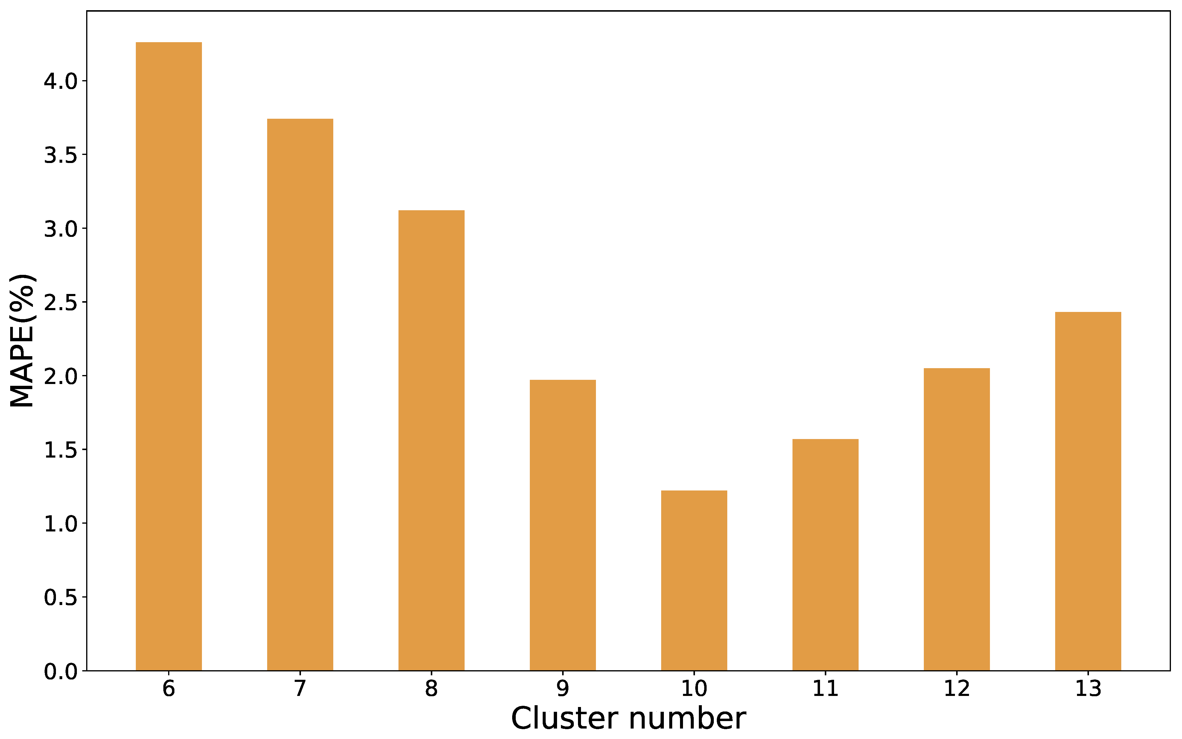
4.2. Comparison of Various k-Values

As mentioned before, we adopted the k-means algorithm to cluster similar days in one group. However, the number of cluster has a significant impact on the algorithm’s performance. So, in the first experiment, we will confirm the idle value of k through evaluating the performance of the k-means algorithm under various k values. The range of the k we assumed in the experiment is from 6 to 13. To prevent the result from being influenced by some other relative factors, such as weather and day type, we chose four weeks from different seasons in 2008 to make the day-ahead load prediction. The prediction result variation trend is similar when k takes different values. we also calculated the value of MAPE for each prediction case to evaluate its performance. The computation result is shown in Figure 10. As we can see, the value of MAPE bottomed out when the k = 10. Based on this result, we select the ten as the final cluster number in our following experiments.

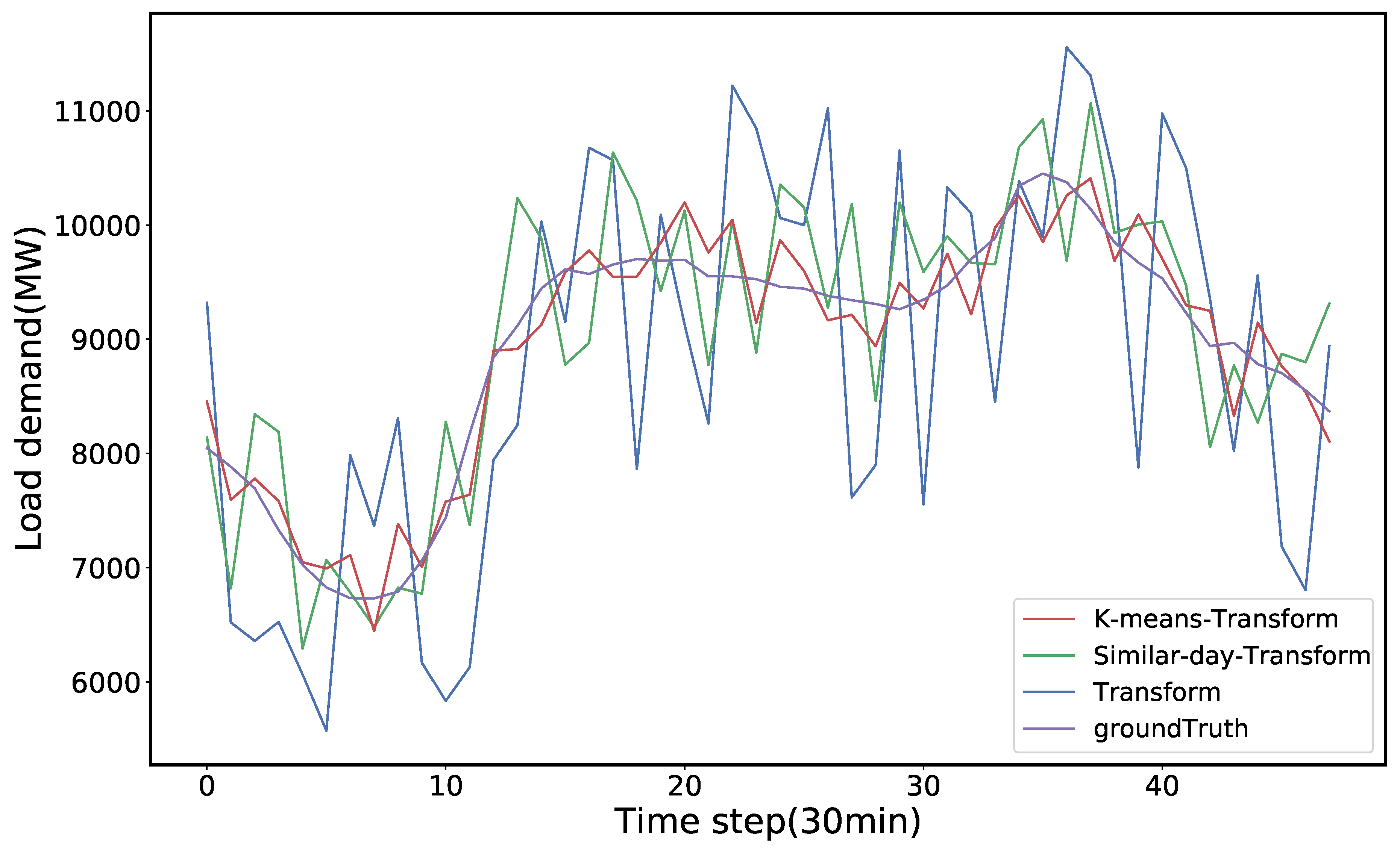
4.3. Evaluation of the Effective of Future Weighted

In our proposed model, we employed LightGBM to assign individual weights to each feature. The individual feature weight aims to reduce the exogenous factors’ influence and avoid slow convergence speed. The technical specifics have been detailed in the above section. To evaluate the effectiveness of the proposed similar day selection approach, we set up a simulation experiment to compare the forecasting performance among k means—transformer-based, LightGBM-k means-transformer-based, transformer-based and ground truth. The following Figure 11 illustrates the different approaches’ electrical load prediction result. The time range in this experiment is one day ahead, which contains 48 samples. The advantage of the similar day selection approach is that it helps the forecasting model avoid becoming trapped into an optimum local area and increases accuracy. Figure 11 illustrates that our proposed approach is closest to the ground-truth value, which proves that the LightGBM model is capable of assigning the individual weight to each feature and helps merge the similar days in one cluster effectively. These experiment results prove the effectiveness of our proposed similar-day selection approach.

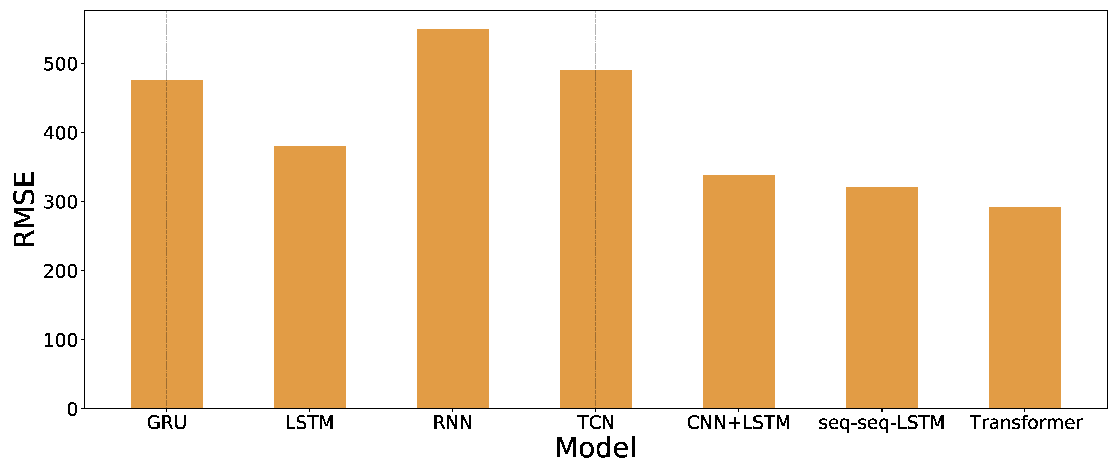
4.4. Forecasting Result

To evaluate our forecasting model’s performance, we conducted a series of simulations, and the results are shown in the following figures and tables. Figure 12 presents the seven models’ average RMSE value in the 2010 day-ahead load forecasting task, and we see that the transformer based model outperforms other baseline models.Figure 13 illustrates the comparison of the day-ahead load prediction result between the proposed model and ground truth. The x-axis in Figure 13 represents the time steps where the y-axis depicts the electricity load. As is exhibited in the graph, the proposed model load forecasting curve follows the ground truth better than the other two approaches. Although these prediction models can forecast the trend of electricity load demand, these models’ forecasting values have a significant error during the peak load period. Furthermore, to avoid the influence of date type and weather conditions, we randomly selected another four days in 2010 from different seasons. Figure 14 demonstrate the our model’s one day ahead load forecasting result using the dataset of NSW. Above all, in most times, we found from these figures that the proposed model outperforms other approaches. On the other hand, our proposed model’s forecasting performance on holiday’s load is outstanding compared to the traditional model. That is because we employed LightGBM and k means algorithm to cluster similar day. On the other hand, we adopt date type, temperature and humidity as supplemental features, which can improve the forecasting performance at different seasons. The following figures illustrate the performance of our proposed model.

To evaluate the performance of our proposed algorithm, we compared our proposed model with various mainstream deep learning based approaches which include convolutional neural networks (CNN), recurrent neural networks (RNN), long short-term memory (LSTM) and hybrid approaches.

Table 1. MAPE of three models in 2010.

Model	Jan	Feb	Mar	Apr	May	June	July	Aug	Sep	Oct	Nov	Dec	Average
GRU	2.78	2.65	2.74	3.54	3.17	3.69	2.93	3.02	3.45	2.71	3.16	2.98	3.06
LSTM	1.81	1.93	2.02	1.65	1.78	1.76	1.86	1.63	1.69	1.79	2.15	1.91	1.93
RNN	4.65	3.89	4.28	3.94	4.58	4.33	3.85	3.62	4.76	3.90	4.13	4.28	4.18
TCN	1.97	2.27	2.02	1.92	1.76	2.12	2.06	1.82	1.95	2.04	1.94	1.89	1.98
CNN + LSTM	1.65	1.72	1.68	1.49	1.52	1.57	1.62	1.53	1.48	1.74	1.46	1.55	1.58
seq2seq-LSTM	1.29	1.35	1.39	1.32	1.28	1.21	1.31	1.19	1.24	1.36	1.31	1.25	1.29
Transformer	1.23	1.46	1.15	0.93	1.09	1.13	1.26	1.12	1.07	1.18	0.96	1.02	1.13

above shows the comparison of average MAPE value among the proposed model and other mainstream approaches when dealing with the same forecasting task.

From Table 1, we can obtain that RNN exhibits satisfactory predictive performance due to its outstanding ability on modelling dynamics in sequential data. On the other hand, compared to the RNN, LSTM performs better due to its strong ability on processing time series data and overcomes the shortage of gradient disappearance and explosion in RNNs.Moreover, the Hybrid methods demonstrate better forecasting ability than LSTM. For instance, in [31], the CNN network is used to transform historical data and extract features for the subsequent load prediction. However, we can obtain from the Table 1 and

Table 2. Wilcoxon signed-rank test results for one day ahead forecasting results.

Compared Models	p-Value
Our proposed model vs. RNN	0.0086
Our proposed model vs. LSTM	0.0145
Our proposed model vs. GRU	0.0001
Our proposed model vs. TCN	0.0197
Our proposed model vs. CNN + LSTM	0.0284
Our proposed model vs. seq2seq-LSTM	0.0336

that our proposed approaches outperforms than all above approaches in both MAPE and RMSE. The average MAPE value day-ahead forecasting can achieve is 1.13 %, while for LSTM it is 1.93%, for RNN it is 4.18%. Comparing with the LSTM model, the MAPE value was reduced by 41.4% and RMSE value was reduced by 24.3%. Even compare with the CNN-LSTM, our proposed model also achieved 28.5% and 13.6% reduced on both MAPE and RMSE. The experiment results showes that self-attention mechanism have favorably ability on learning complex patterns and dynamics from time series data. Furthermore, the experiment results also proves that the self-attention mechanism in transformer model have better performance on capturing complex dynamic patterns than linear attention mechanism which adopted by seq2seq.

As we mentioned before, the electricity load can be affected by various factors such as seasonal, temperature etc. So we can obtain from the table that the proposed model’s performance fluctuates in different seasons. Figure 11 and Figure 13 indicate that the high peak load point is located during night time. The average load in summer is higher than the other three seasons, which may caused by the usage of home appliances. As we can see, our proposed model’s prediction curve is closest to the real load most time. The experiment results prove that the similar day selection approach is essential and effective.In addition, to confirm the validity and the statistical significance of our proposed model, we employ Wilcoxon signed-rank test, in which the significance level of $\alpha$ is 0.05. Table 2 illustrate the test result, which shows that our proposed model outperformed other baselines.

5. Conclusions

Accurate STLF plays a significant role in plans for electricity generation and distribution in the smart grid. This chapter introduces a novel model based on the transformer network to provide an accurate day-ahead load forecasting result. Furthermore, our model also combines a similar day selection approach, which involves LightGBM and k-means algorithm. In our model, LightGBM is employed to calculate each supplemental feature’s individual weight, and the k-means algorithm is applied to classify similar days in one cluster. The demonstration results prove that the similar day selection approach can enhance the model’s forecasting performance effectiveness. On the other hand, Transformer is applied to forecast the day-ahead load. To verify our model’s performance, we set up a series of simulation experiments with average mean absolute percentage error (MAPE) as the error criteria. The test data is the electricity consumption data in Australia in 2010, which was provided by AEMO. The demonstrated result proved that our proposed model outperforms other mainstream approaches with regard to forecasting accuracy. In our proposed model, the MAPE is 1.13, while for RNN is 4.18, LSTM it is 1.93. Compare to the traditional approaches, our proposed model is more reliable owing to its outstanding performance on holiday load prediction.

The proposed model’s prediction performance during the peak period is still unsatisfactory and needs to be improved. Based on the comparative research and the transformer’s characteristic, in the next step, we will focus on developing a hybrid forecasting model that combines the CNN with the transformer. On the other hand, some studies point out that utilising the day-ahead peak as the relevant feature can reduce forecasting errors during the peak period. In the future, we should try to add more relevant features to our model. Furthermore, we will attempt to employ some advanced signal processing techniques to enhance the effectiveness of feature extraction.

References

1. Heinemann, G.T.; Nordmian, D.A.; Plant, E.C. The Relationship Between Summer Weather and Summer Loads—A Regression Analysis. IEEE Trans. Power Appar. Syst. 1966, PAS-85, 1144–1154. [Google Scholar] [CrossRef]
2. Samuel, I.A.; Adetiba, E.; Odigwe, I.A.; Felly-Njoku, F.C. A comparative study of regression analysis and artificial neural network methods for medium-term load forecasting. Indian J. Sci. Technol. 2017, 10, 1–7. [Google Scholar] [CrossRef]
3. Hobbs, B.F.; Jitprapaikulsarn, S.; Konda, S.; Chankong, V.; Loparo, K.A.; Maratukulam, D.J. Analysis of the value for unit commitment of improved load forecasts. IEEE Trans. Power Syst. 1999, 14, 1342–1348. [Google Scholar] [CrossRef]
4. Kalekar, P.S. Time series forecasting using holt-winters exponential smoothing. Kanwal Rekhi Sch. Inf. Technol. 2004, 4329008, 1–13. [Google Scholar]
5. Che, J.; Wang, J. Short-term electricity prices forecasting based on support vector regression and auto-regressive integrated moving average modeling. Energy Convers. Manag. 2010, 51, 1911–1917. [Google Scholar] [CrossRef]
6. Ye, N.; Liu, Y.; Wang, Y. Short-term power load forecasting based on SVM. In Proceedings of the World Automation Congress 2012, Puerto Vallarta, Mexico, 24–28 June 2012; pp. 47–51. [Google Scholar]
7. Ranaweera, D.; Hubele, N.; Karady, G. Fuzzy logic for short term load forecasting. Int. J. Electr. Power Energy Syst. 1996, 18, 215–222. [Google Scholar] [CrossRef]
8. Badri, A.; Ameli, Z.; Birjandi, A.M. Application of artificial neural networks and fuzzy logic methods for short term load forecasting. Energy Procedia 2012, 14, 1883–1888. [Google Scholar] [CrossRef] [Green Version]
9. Amber, K.; Aslam, M.; Hussain, S. Electricity consumption forecasting models for administration buildings of the UK higher education sector. Energy Build. 2015, 90, 127–136. [Google Scholar] [CrossRef]
10. Song, K.B.; Baek, Y.S.; Hong, D.H.; Jang, G. Short-term load forecasting for the holidays using fuzzy linear regression method. IEEE Trans. Power Syst. 2005, 20, 96–101. [Google Scholar] [CrossRef]
11. Amral, N.; Ozveren, C.S.; King, D. Short term load forecasting using Multiple Linear Regression. In Proceedings of the 2007 42nd International Universities Power Engineering Conference, Brighton, UK, 4–6 September 2007; pp. 1192–1198. [Google Scholar] [CrossRef]
12. Silva, G.C.; Silva, J.L.R.; Lisboa, A.C.; Vieira, D.A.G.; Saldanha, R.R. Advanced fuzzy time series applied to short term load forecasting. In Proceedings of the 2017 IEEE Latin American Conference on Computational Intelligence, (LA-CCI), Arequipa, Peru, 8–10 November 2017; pp. 1–6. [Google Scholar] [CrossRef]
13. Adika, C.O.; Wang, L. Short term energy consumption prediction using bio-inspired fuzzy systems. In Proceedings of the 2012 North American Power Symposium (NAPS), Champaign, IL, USA, 9–11 September 2012; pp. 1–6. [Google Scholar] [CrossRef]
14. Noble, W.S. What is a support vector machine? Nat. Biotechnol. 2006, 24, 1565–1567. [Google Scholar] [CrossRef]
15. Zhang, M.-G. Short-term load forecasting based on support vector machines regression. In Proceedings of the 2005 International Conference on Machine Learning and Cybernetics, Guangzhou, China, 18–21 August 2005; Volume 7, pp. 4310–4314. [Google Scholar] [CrossRef] [Green Version]
16. Amin, M.A.A.; Hoque, M.A. Comparison of ARIMA and SVM for Short-term Load Forecasting. In Proceedings of the 2019 9th Annual Information Technology, Electromechanical Engineering and Microelectronics Conference (IEMECON), Jaipur, India, 13–15 March 2019; pp. 1–6. [Google Scholar] [CrossRef]
17. Xiao, Z.; Ye, S.J.; Zhong, B.; Sun, C.X. BP neural network with rough set for short term load forecasting. Expert Syst. Appl. 2009, 36, 273–279. [Google Scholar] [CrossRef]
18. Bin, H.; Zu, Y.X.; Zhang, C. A forecasting method of short-term electric power load based on BP neural network. Appl. Mech. Mater. 2014, 538, 247–250. [Google Scholar] [CrossRef]
19. Chen, S.T.; Yu, D.C.; Moghaddamjo, A.R. Weather sensitive short-term load forecasting using nonfully connected artificial neural network. IEEE Trans. Power Syst. 1992, 7, 1098–1105. [Google Scholar] [CrossRef]
20. Chen, K.; Chen, K.; Wang, Q.; He, Z.; Hu, J.; He, J. Short-Term Load Forecasting With Deep Residual Networks. IEEE Trans. Smart Grid 2019, 10, 3943–3952. [Google Scholar] [CrossRef] [Green Version]
21. Lara-Benítez, P.; Carranza-García, M.; Luna-Romera, J.M.; Riquelme, J.C. Temporal convolutional networks applied to energy-related time series forecasting. Appl. Sci. 2020, 10, 2322. [Google Scholar] [CrossRef] [Green Version]
22. Amarasinghe, K.; Marino, D.L.; Manic, M. Deep neural networks for energy load forecasting. In Proceedings of the 2017 IEEE 26th International Symposium on Industrial Electronics (ISIE), Edinburgh, UK, 19–21 June 2017; pp. 1483–1488. [Google Scholar] [CrossRef]
23. Siddarameshwara, N.; Yelamali, A.; Byahatti, K. Electricity Short Term Load Forecasting Using Elman Recurrent Neural Network. In Proceedings of the 2010 International Conference on Advances in Recent Technologies in Communication and Computing, Kottayam, India, 16–17 October 2010; pp. 351–354. [Google Scholar] [CrossRef]
24. Marvuglia, A.; Messineo, A. Using recurrent artificial neural networks to forecast household electricity consumption. Energy Procedia 2012, 14, 45–55. [Google Scholar] [CrossRef] [Green Version]
25. Kong, W.; Dong, Z.Y.; Jia, Y.; Hill, D.J.; Xu, Y.; Zhang, Y. Short-Term Residential Load Forecasting Based on LSTM Recurrent Neural Network. IEEE Trans. Smart Grid 2019, 10, 841–851. [Google Scholar] [CrossRef]
26. Zheng, J.; Xu, C.; Zhang, Z.; Li, X. Electric load forecasting in smart grids using Long-Short-Term-Memory based Recurrent Neural Network. In Proceedings of the 2017 51st Annual Conference on Information Sciences and Systems (CISS), Baltimore, MD, USA, 22–24 March 2017; pp. 1–6. [Google Scholar] [CrossRef]
27. Cheng, Y.; Xu, C.; Mashima, D.; Thing, V.L.; Wu, Y. PowerLSTM: Power demand forecasting using long short-term memory neural network. In Proceedings of the International Conference on Advanced Data Mining and Applications, Singapore, 5–6 November 2017; pp. 727–740. [Google Scholar]
28. Bouktif, S.; Fiaz, A.; Ouni, A.; Serhani, M.A. Optimal deep learning lstm model for electric load forecasting using feature selection and genetic algorithm: Comparison with machine learning approaches. Energies 2018, 11, 1636. [Google Scholar] [CrossRef] [Green Version]
29. Wang, Y.; Liu, M.; Bao, Z.; Zhang, S. Short-term load forecasting with multi-source data using gated recurrent unit neural networks. Energies 2018, 11, 1138. [Google Scholar] [CrossRef] [Green Version]
30. Stollenga, M.F.; Byeon, W.; Liwicki, M.; Schmidhuber, J. Parallel multi-dimensional LSTM, with application to fast biomedical volumetric image segmentation. arXiv 2015, arXiv:1506.07452. [Google Scholar]
31. He, W. Load forecasting via deep neural networks. Procedia Comput. Sci. 2017, 122, 308–314. [Google Scholar] [CrossRef]
32. Tian, C.; Ma, J.; Zhang, C.; Zhan, P. A deep neural network model for short-term load forecast based on long short-term memory network and convolutional neural network. Energies 2018, 11, 3493. [Google Scholar] [CrossRef] [Green Version]
33. Marino, D.L.; Amarasinghe, K.; Manic, M. Building energy load forecasting using Deep Neural Networks. In Proceedings of the IECON 2016—42nd Annual Conference of the IEEE Industrial Electronics Society, Florence, Italy, 23–26 October 2016; pp. 7046–7051. [Google Scholar] [CrossRef] [Green Version]
34. Ke, G.; Meng, Q.; Finley, T.; Wang, T.; Chen, W.; Ma, W.; Ye, Q.; Liu, T.Y. Lightgbm: A highly efficient gradient boosting decision tree. Adv. Neural Inf. Process. Syst. 2017, 30, 3146–3154. [Google Scholar]
35. MacQueen, J. Some methods for classification and analysis of multivariate observations. In Proceedings of the Fifth Berkeley Symposium on Mathematical Statistics and Probability, Oakland, CA, USA, 21 June–18 July 1967; Volume 1, pp. 281–297. [Google Scholar]
36. Mnih, V.; Heess, N.; Graves, A.; Kavukcuoglu, K. Recurrent models of visual attention. arXiv 2014, arXiv:1406.6247. [Google Scholar]
37. Vaswani, A.; Shazeer, N.; Parmar, N.; Uszkoreit, J.; Jones, L.; Gomez, A.N.; Kaiser, L.; Polosukhin, I. Attention is all you need. arXiv 2017, arXiv:1706.03762. [Google Scholar]
38. Abadi, M.; Barham, P.; Chen, J.; Chen, Z.; Davis, A.; Dean, J.; Devin, M.; Ghemawat, S.; Irving, G.; Isard, M.; et al. Tensorflow: A system for large-scale machine learning. In Proceedings of the 12th {USENIX} Symposium on Operating Systems Design and Implementation ({OSDI} 16), Savannah, GA, USA, 2–4 November 2016; pp. 265–283. [Google Scholar]
Figure 1. Load demand variation in one week.
Information 12 00516 g001
Figure 2. Load demand and humidity data in 10 May 2006.
Information 12 00516 g002
Figure 3. Load demand and temperature data in 10 May 2006.
Information 12 00516 g003
Figure 4. The entire architecture of the forecasting system.
Information 12 00516 g004
Figure 5. The relevance score of each factors.
Information 12 00516 g005
Figure 6. Attention mechanism.
Information 12 00516 g006
Figure 7. The architecture of the encoder and decoder in the transformer model.
Information 12 00516 g007
Figure 8. The specific architecture of encoder and decoder.
Information 12 00516 g008
Figure 9. The specific architecture of positional encoding.
Information 12 00516 g009
Figure 10. MAPE (%) for various cluster number.
Information 12 00516 g010
Figure 11. Day-ahead prediction of various model (date 2 September 2010).
Information 12 00516 g011
Figure 12. The average RMSE in 2010 load forecasting for seven models.
Information 12 00516 g012
Figure 13. Mainstream algorithms day-ahead prediction performance comparsion (date 12 September 2010).
Information 12 00516 g013
Figure 14. Day-ahead prediction of transformer-based model in different seasons.
Information 12 00516 g014