Article

Heuristic Analysis for In-Plane Non-Contact Calibration of Rulers Using Mask R-CNN

by
Michael Telahun
*,
Daniel Sierra-Sossa
and
Adel S. Elmaghraby
Department of Computer Science and Engineering, University of Louisville, Louisville, KY 40292, USA
*
Author to whom correspondence should be addressed.
Information 2020, 11(5), 259; https://doi.org/10.3390/info11050259
Submission received: 9 April 2020 / Revised: 25 April 2020 / Accepted: 6 May 2020 / Published: 9 May 2020

Abstract

:
Determining an object measurement is a challenging task without having a well-defined reference. When a ruler is placed in the same plane of an object being measured it can serve as metric reference, thus a measurement system can be defined and calibrated to correlate actual dimensions with pixels contained in an image. This paper describes a system for non-contact object measurement by sensing and assessing the distinct spatial frequency of the graduations on a ruler. The approach presented leverages Deep Learning methods, specifically Mask Region proposal based Convolutional Neural Networks (R-CNN), for rulers’ recognition and segmentation, as well as several other computer vision (CV) methods such as adaptive thresholding and template matching. We developed a heuristic analytical method for calibrating an image by applying several filters to extract the spatial frequencies corresponding to the ticks on a given ruler. We propose an automated in-plane optical scaling calibration system for non-contact measurement.

1. Introduction

Non-contact object measurement has a long history of applications in several fields of industry and study. A few applications include measuring industrial fractures/cracks [1], measuring plant/leaf size [2], wound morphology [3], forensics [4], and archaeology [5]. Non-contact object measurement refers to the measuring of objects via a method or device which does not interrupt or come in contact with the object of focus. This can either be done with a device in real time, or via software, after an image of the object is captured. To measure captured images a reference or proxy marker is often used to spatially calibrate the resolution of the image [6,7]. In this sense, a graduated device or ruler placed in close proximity can also be used to better spatially comprehend the contents of an image. Therefore a reference marker, specifically a ruler, can be used to spatially register the size of the contents in an image. For these images, the digital measurement in pixels (px) and the spatial reference marker, such as a ruler, would need to be captured in the same plane and then measured. A common metric for the combination of these two measurements is dots per inch (DPI) which is the number of pixels per inch.
Often, measuring an image in pixels involves manual work somewhere in the pipeline and in order to maintain a confident level of accuracy/consistency the task becomes time consuming, disregarding the abilities of semantic segmentation [8,9] momentarily. Dynamically or automatically achieving this level of image calibration would over come two limitations. The first is that manually measuring each image in a database can take a lot of human hours. The second is that manual measurement induces subjectivity to the task which is objective in nature, meaning different measurements will be retrieved by different people for the same image. This second hurdle can be evaluated by considering the aforementioned applications’ individual needs for consistently accurate measurements.
In this work, we chose to implement non-contact object measurement for images containing rulers. This is primarily because rulers are well standardized and readily available in common practice. This system can be used to either automatically convert pixel measurements for an image with an object and a ruler or to manually measure elements with the generated graduation to pixel ratio. However, if measurements are provided, the system is able to take the objects morphological data, measured in pixels, and convert it to whichever graduation system was provided.
This system is capable of calculating the graduation to pixel ratio in DPI or DPM (dots per millimeter) of an image provided it contains a ruler. To do this, we created a heuristic technique for approximating the distances between the graduations on a ruler. In this work the resulting measurement in pixels from one graduation to another translates to the mode of the spatial frequencies along a region of a ruler, which identifies the element that occurs most often in the spatial frequencies set.
Hough Transforms have been cited as perhaps the most popular technique for measuring rulers in images for determining scale and measuring objects. Hough lines are extracted following a similar methodology to edge detection and often involve some initial metric of edges to retrieve a result. Although it is a very straightforward solution to the problem, it typically requires specific parameters for different rulers and images. One system which uses the Hough transform to detect measurement tools such as rulers and concentric circles of fixed radii [10] was developed. This system works by gathering several regions with vertical lines with respect to a large horizontal line. The filtering of the method looks at sample mean, variance and standard deviation to evaluate the weighted input information for graduations on a ruler. The specified inputs to the system are the type of ruler, the graduation distances, and the minimum number of elements to be considered [10]. For the two images listed in their paper under the results section given for manual vs semi-automatic the measurements varied from 2.3 mm to 0.027 mm.
Another method which uses the Hough transform in forensics [11] extracts the spatial frequencies of a ruler first by using a two-dimensional Discrete Fourier Transform (2-D DFT) which is modeled after a known ruler. Both this methodology and Calatron’s et al. [10] method are largely similar for extracting the graduation distances, although here the evaluation is done using a block based DFT. This method is capable of sampling at a sub-pixel level, this is a necessity when assessing some forensic samples such as finger prints [11]. Additionally, this method appears to only work specifically for forensic rulers which have very unique features. Our system was not targeted for one particular reference ruler, thereofore we chose to forgo Hough transforms as it would only narrow the solution to a specific category or ruler type.
Object detection and recognition have been major topics of computer vision with a variety of solutions addressing several problems such as: character recognition, semantic segmentation, self-driving cars, and visual search engines [12,13,14,15,16]. In brief, object detection is a way to identify whether or not instances of an object are contained in an image [17], and object recognition a way to classify an object given a label that characterizes that object [18]. State of the art solutions for object detection and recognition today rely on one or a few combinations of deep neural network techniques. In particular, Region proposal based Convolutional Neural Networks (R-CNN) [19] are among the most proficient. Others, such as You Only Look Once (YOLO) [20], Fast YOLO [21], Single Shot Detector (SSD) [22], Neural Architecture Search Network (NASNet) [23], and Region-based Fully Convolutional Network (R-FCN) [24] apply different approaches. These discoveries/optimizations along with advances in R-CNNs occured all in a relatively short period of just a few years. Enhancements to the standard R-CNN architecture, such as Fast R-CNN [25], Faster R-CNN [26], and Mask R-CNN (MRCNN) [27] have led to improved speed, accuracy, and other benefits in the realm of object detection/recognition [28,29].
Year over year we see that smartphone devices and cameras are used for an increasing number of smart technologies and applications. Our heuristic system uses a combination of methods as a novel solution for detecting and measuring rulers to scale objects in the same plane. The capacity for our system is made possible by taking advantage of the high resolution images that have become the norm over the past few years. Our proposed method can be split into two distinct pieces in order to achieve heuristic analysis for in-plane non-contact calibration of rulers. First, we perform semantic segmentation by adapting the Mask R-CNN architecture which extracts the area containing a ruler. In Figure 1 this area is represented as “Segmented Result” which is where the proposed heuristic method begins to assess the ruler. We then perform the in-plane non-contact measurement of the segmented ruler returning a calibrated measurement, the architecture in this figure represents the proposed method end to end. In the Section 3 and Section 4, we will expand on the outcome of region for “Pixel Conversion” which is an integer given as pixels per unit of measurement, e.g., pixels per millimeter.

2. Materials and Methods

In this section we describe our database, which was used for both training and validating the Mask R-CNN model. The same dataset was used in the development and testing of the calibration method. Then, we briefly provide an overview of our adaptation to Mask R-CNN for instance segmentation and object detection, and how we interpret its outputs for the calibration method. Finally, we describe in detail the procedure for our proposed heuristic calibration method of a ruler.

2.1. Resources—Database

To create the database, we segmented and labeled images containing rulers from a proprietary dataset. To perform the segmentation a semi-automated segmentation tool was created for generating binary masks and their corresponding JavaScript Object Notation (JSON) mapping. The semi-automated tool allows the user to plot points by using a mouse. In real time, the software will draw a line connecting these two points together. The points from the user and the line created bound the segmented object and correspond to regions. These regions are converted into a JSON object and is used as the ground truth for MRCNN. In total, 430 images were segmented and labeled, 322 images were used for training and the remaining 108 were used to validate the model. Some images in our database contain artifacts such as hands or clothes that interfere or cover parts of the rulers. We include these images for a more realistic outcome from the training. Each ruler was marked with the class “Ruler” to denote the segmented object or region contained within that image. Images in our database had image resolutions ranging from 800 × 525 pixels to 5184 × 3456 pixels. Across the entire dataset 61.2% of the images were larger then 1920 × 1080 pixels and 4.66% of the images were 800 × 525 pixels. These images were taken with a variety of devices including smart phones. We did not personally procure this database it was provided by a third party source.

2.2. Mask R-CNN Adaptation for Ruler Segmentation

Within the field of computer vision, semantic segmentation provides a way for separating or extracting objects within an image by classifying several small groups of pixels that correlate to a larger single group or class [9,30]. Mask R-CNN, a popular extension of Faster R-CNN (FRCNN), an architecture for object instance segmentation, has the capacity to perform semantic segmentation, object localization or classification, and masking [27]. This architecture won the COCO dataset challenge in 2017 and has been adapted to many different datasets with top of the line results [28,29,31,32,33,34]. This architecture makes several improvements to FRCNN, one of these is how regions of interest (RoI) are used within the model, improving the instance segmentation of FRCNN by the application of what they call RoIAlign, a feature map RoI identifier that computes the value of each sampling point using bilinear interpolation from the adjacent grid points [27]. A second improvement comes from the addition of a fully convolutional network or FCN to perform the masking which occurs in parallel with the classification and bounding box extraction. The FCN [9] makes use of a Feature Pyramid Network or FPN [35] which performs the feature extraction for the classification. This is then used to propose the bounding box around the object of interest, which is essential to our method because it gives us with high confidence the square area containing a ruler. The ‘Mask’ in Mask R-CNN is the last improvement to the FRCNN model we will discuss, and it is the reason we chose to use MRCNN in our system. As an output the model will produce a binary mask containing the area of the object of focus, in this paper that is the area of the ruler, based on the prediction for the class and RoIs. This follows from making several region proposals with different sizes around each instance of an object. The mask generated consists of m × m masks generated from the FCN and it is structured by the RoI-Align [27].
The binary mask is our preferred target output of Mask R-CNN, as it will provide the least amount of noise with the maximum amount of information needed for our system to calibrate an image. With the mask we can extract only the ruler from the original image and then immediately perform our calibration method. However this procedure is not perfect so we additionally take advantage of the bounding box which will contain enough of a ruler for the calibration method to execute. The calibration method we propose is also capable of handling outputs of this type. In Figure 1 a bounding box result is used to show the full scope of the architecture. In Figure 2, masks are used to show the capability of Mask R-CNN and why it is used in this paper for extracting a ruler from an image. We applied some constraints to the bounding box output and discuss the drawbacks in Section 2.3 but still consider it as an acceptable intermediate outcome of our system.

2.3. Heuristic Scale Calibration

To generate the calibrated output, our method follows three steps: Preparation, Deep Searching, and Calibration/Conversion. Each of these steps or components and their contribution to the system can be seen in Figure 2. In addition, in this figure, preparation, the output of Mask R-CNN can be seen as either a segmented ruler or a bounding box. The preparation step includes cropping, down-sampling, removal of noise, and testing the image for spatial frequencies before the deep search. In the deep search, the method will search the ruler by looking for spatial frequencies corresponding to the graduations or ticks on a ruler.
In the validation, the last part of Figure 2, the target system and calibration, or conversion from pixels, is performed. This is a mapping of the number of ticks in a region to the number of pixels expected for the equivalent space. We assume the calibrated output will be a measurement in the metric or imperial system because we expect a visible and referenceable ruler contained in the image.

2.3.1. Preparation

Preparing the Mask R-CNN result for the deep search starts with a simple test to determine if the image has any spatial frequencies that can be searched. This test is a lite version of the Deep Searchbut gives adequate indication whether the output is searchable. The decision of this step is based on the detection score achieved using MRCNN. In short if the test fails we know that there was very few spatial frequencies in the Mask R-CNN result, one example of this is a picture of a plain surface. In the event that there is no mask, the system will default to searching the bounding box from here on. A search on the bounding box is slower, as the search window will include excess area of background. The amount of background acceptable for searching with our method should be less than roughly two times the area of the ruler. Decreased performance is expected when the background is large as the search would take too long to process. We will refer to the resulting image from MRCNN as the RulerImage. The RulerImage is then converted to grayscale and template matching is performed. Template matching in this process is used to reduce the search area to a small window of the ruler to one dense region of graduations, which we will call the TemplateWindow. The TemplateWindow can be seen in Figure 2. The TemplateWindow is the only area region of the image that is searched for in the Deep Search. For template matching, we use the Template Matching Correlation Coefficient T M _ C C O E F F , which slides through an image and seeks the best sum of pixel intensities closest to the template following 2D convolution [36].
A patch or window of size w × h from the image denoted I is compared against a template denoted T , creating an array set of results that represent the matches [36]. The best match is selected with T M _ C C O E F F which chooses the best matrix denoted R ( x , y ) as the comparison with the points and their position having the global maximum. The template ruler was manually created and designed with the dimensions of a metric ruler; however, our system can identify an imperial ruler with the same template. The size of the TemplateWindow is bounded between 150 × 150 to 500 × 500 px and its value is calculated based on the size of the RulerImage, this is to reduce computing time. The size of the TemplateWindow is initially calculated as the length of the shortest dimension of the segmented result. It is then incrementally reduced to fit in the aforementioned bounds. The size reflects the pixel density of the image where 500 px corresponds to images larger than 2560 × 1440 px. The lower bound is the minimum resolution the system can search with and is used for images as small as 800 × 525 px. To finish preparations for the deep search the image is converted to black and white using adaptive thresholding. We chose this method over others, such as Otsu Method (https://www.mdpi.com/search?q=otsu), because it does not look at the global values of the image. Adaptive thresholding converts a gray scale image to black and white by splitting the image into windows and taking the local minimum/maximum of the window. The method for adaptive thresholding in OpenCV (Open Computer Vision) [36] takes a thresholding method as a parameter such as Otsu but for our system Binary thresholding was used. In our system we used ADAPTIVE_THRESH_GAUSSIAN_C as the thresholding method because it takes the weighted sum of the neighborhood instead of the mean [36]. The mean value produces results closer to the Otsu method which only considers the mean value of the image. For the purpose of removing localized noise we used the Gaussian_C method to ensure better results. The window size must also be specified by a kernel, space similar to convolution. Adaptive thresholding has other uses such as edge/object detection [29] and feature extraction/segmentation [37,38,39].

2.3.2. Deep Searching

We define a simple computer vision definition for the graduations on a ruler, in our system, as the region in any RulerImage or TemplateWindow with the highest uniform spatial frequency pattern. The spatial frequency f is defined below as the number of graduations or ticks under a line given the width of black pixels w i within a threshold t.
f = | { i { 1 , 2 , . . . , n } : w i + t } |
To search for this region, we start by creating an array or line with N number of points where 150 < = N < = 500 , the exact value is the width of the TemplateWindow. This value is found in Section 2.3.1. We chose this range based on the variable image size in our database and therefore each TemplateWindow is between 150 × 150 and 500 × 500 pixels. The lower bound of 150 we select to maintain a level of fidelity in the image which should be considered when initially capturing the image. The upper bound of 500 was selected because it is big enough to perform a thorough search on large images and small enough to still execute quickly. The search is repeated for each of the corners in the TemplateWindow such that each corner searches in a 90 degree arc about the image. This is demonstrated in Figure 2 as the InitalSearch. Each of the search parameters are based on the size of the image, where the number of searches is equal to
s e a r c h e s = i X N R
where X is the width of the image, N is the image width of the target image size, R is the quotient of N over 500, and i is the search iterator. The value i is used to incrementally reduce the search space this is because we expect to iteratively improve. Every search has a window or width equal to:
s e a r c h W i n d o w = | X X m R i |
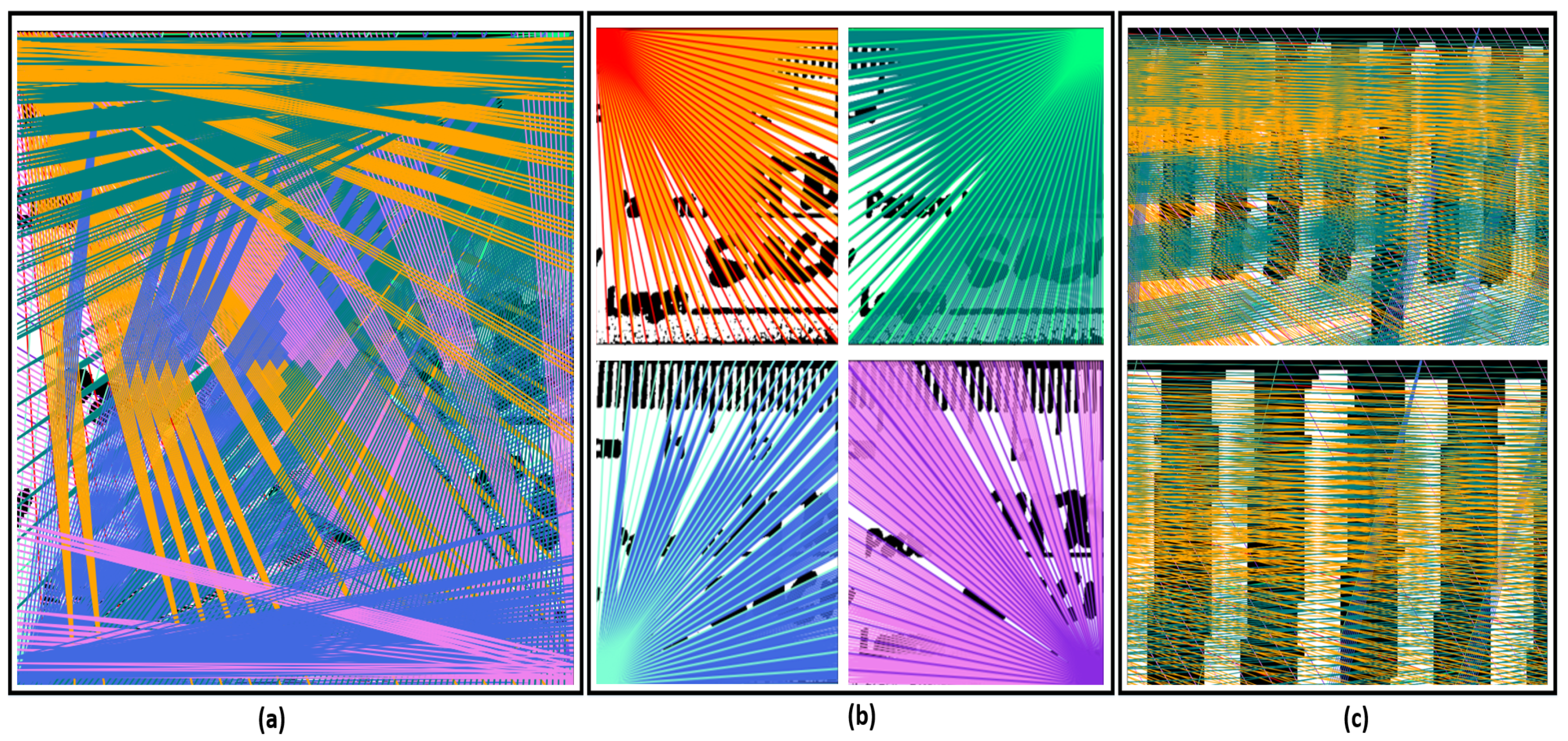
where m is a constant based on the target image size. We selected the constant m based on the target RulerImage size such that the number of searches and search windows would be proportional to the size of the RulerImage. These constants ensures that even if a TemplateWindow is very small, i.e., 150 × 150 pixels, the image will still get searched. After each iteration of the search, the window size and searches per window decreases. Figure 3a presents the combined rendering of the Deep Search method. In Figure 3b each of the regions have been rendered separately noting the empty or white areas where the search stopped or skipped searching altogether. In Figure 3c the rendering shows two zoomed arbitrary regions of Figure 4a where the ticks on the ruler are located, noting the increased number of searches in this small region.
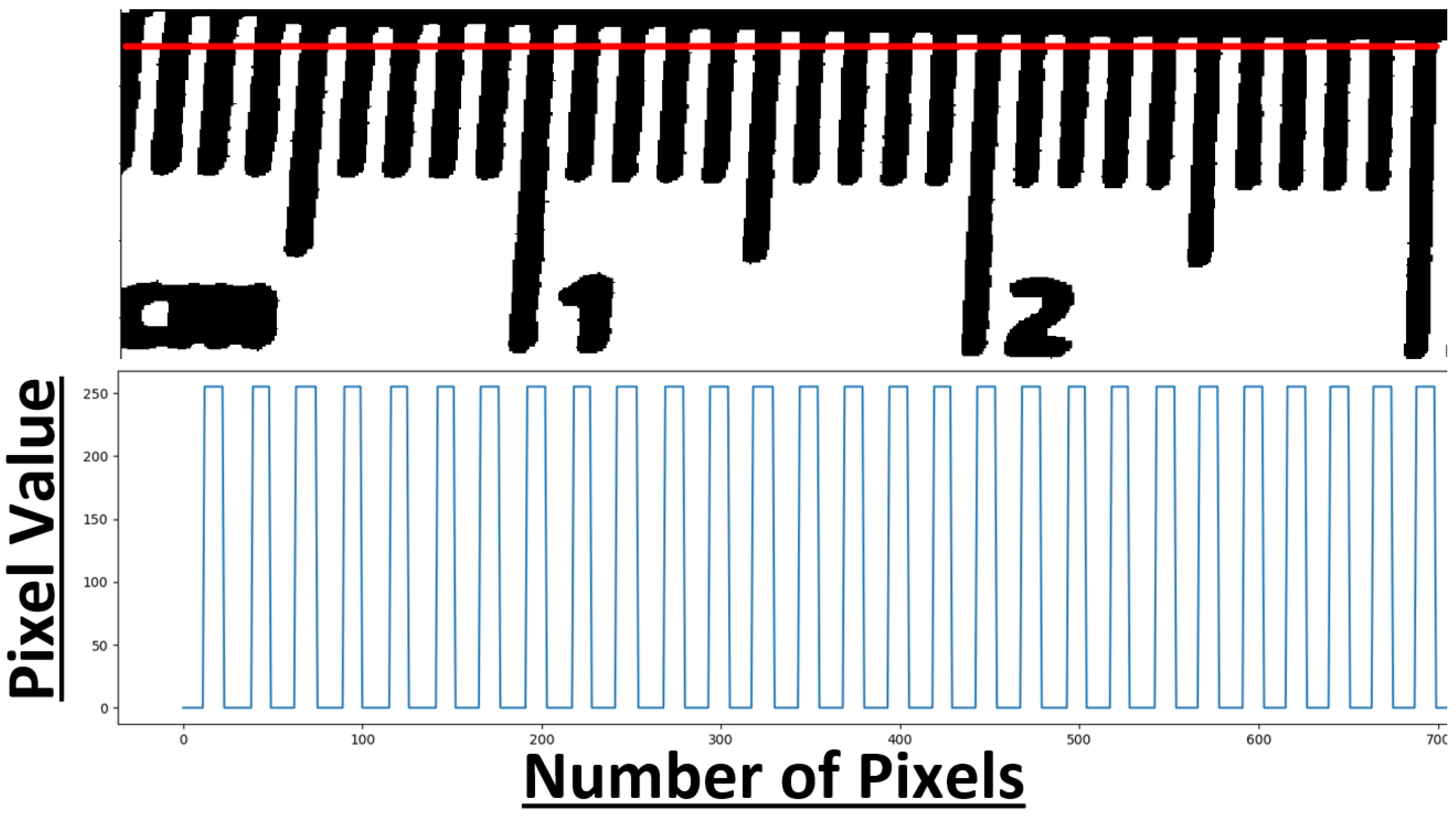
After each search the list of results is filtered to determine if the average number of graduations or spatial frequencies has improved. The first filter will remove results that were less than the average uniform spatial frequency, from Equation (1), in the most recent search. The second filter removes results with a large slope with respect to both the vertical and horizontal axis. The two filters will drop on average half of the search results. The deep search is looking for the improved spatial frequency over each iteration of results. The conclusion of the search will occur when either of the following is true: (1) the search has gone on for too long or (2) the average uniform spatial frequency has not changed. The limited number of searches is meant to provide an extensive yet deterministic result as there could be marginal improvement over many searches. From experimentation, the first condition typically means there was no good result to pick. Meaning the image was not very clear. An unchanged average uniform spatial frequency or the same number of measured graduations is the desired outcome of the deep search where there will either be only one spatial frequency, or a set of spatial frequencies equivalent to the average. In the worst case, the average spatial frequency could decrease after a search. In this scenario, we resort to memoization (https://en.wikipedia.org/wiki/Memoization) and expect the best result to exist in the previous search. When the search exhausts all the available options we retrieve a single spatial frequency. The red line in Figure 4 is the final resulting line and its corresponding spatial frequency is below. In the final calculation we consider both the black and white values for width in the length of a single graduation. We measure the value for a single graduation as M f where M f is the sum of the modes for the black spatial frequency M b and white spatial frequency M w .
M f = M b + M w w h e r e : M b = m ( f b ) a n d : M w = m ( f w )
where we expect M f is one millimeter in the metric system or 1 16 of an inch in the imperial system.

2.3.3. Calibration

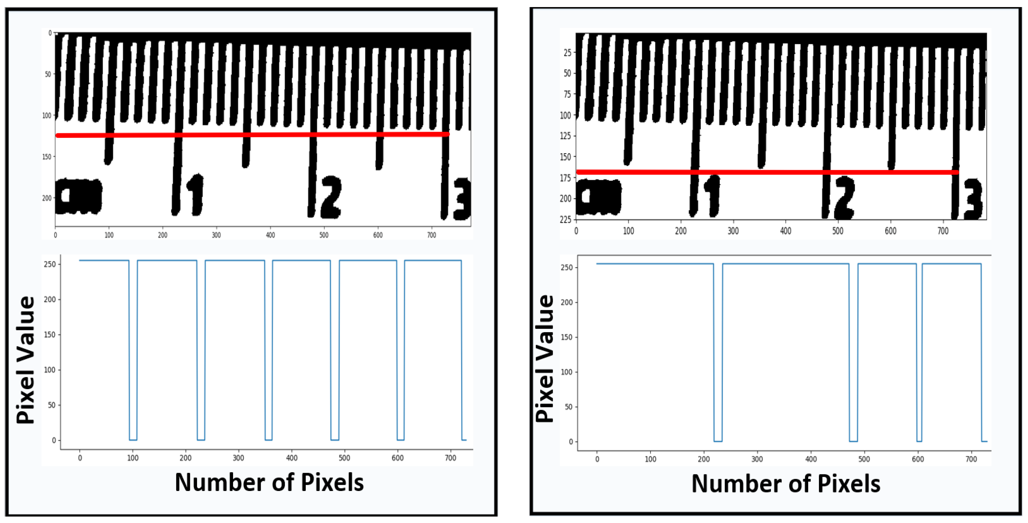
The final calibration of the image is performed immediately following the deep search. To do this the resulting line of the search slides vertically or horizontally through the TemplateWindow to search for spatial frequencies with the same period. The results in Figure 5 are calibrated based on the system where graduations are grouped based on 5 or 10 mm in the metric system and 1 2 or 1 inch in the imperial system. This calibration can be thought of as moving/pivoting the line gradually until it is perpendicular to the graduations to finda a spacial frequency correlated M f . Although, the term perpendicular is used to help explain the procedure, there is no trigonometric function in this procedure. The line we are using to evaluate the system of measure is the result of a heuristic search that uses two pixels per iteration for pivoting to identify a line with the least error in the frequency distribution. This leads to a line that approximates to a 90° angle between the markers and the evaluating line. In Figure 5 the line is almost perpendicular and was the best found by the heuristic system in this case. The spatial frequencies shown in Figure 5 are evaluated as 5 M f on the left and 10 M f on the right. These two definitions are redundant to ensure confidence in the calibrated results when it is possible. The smaller of the two additional spatial frequencies, 5 mm and 1 2 in, should be measured an equal number of times in the calibration step to also retain confidence in a single measure. This number is calculated also based on M f as the number of spatial frequencies in the deep search result over the length of 5 mm or 1 2 inch.

3. Results

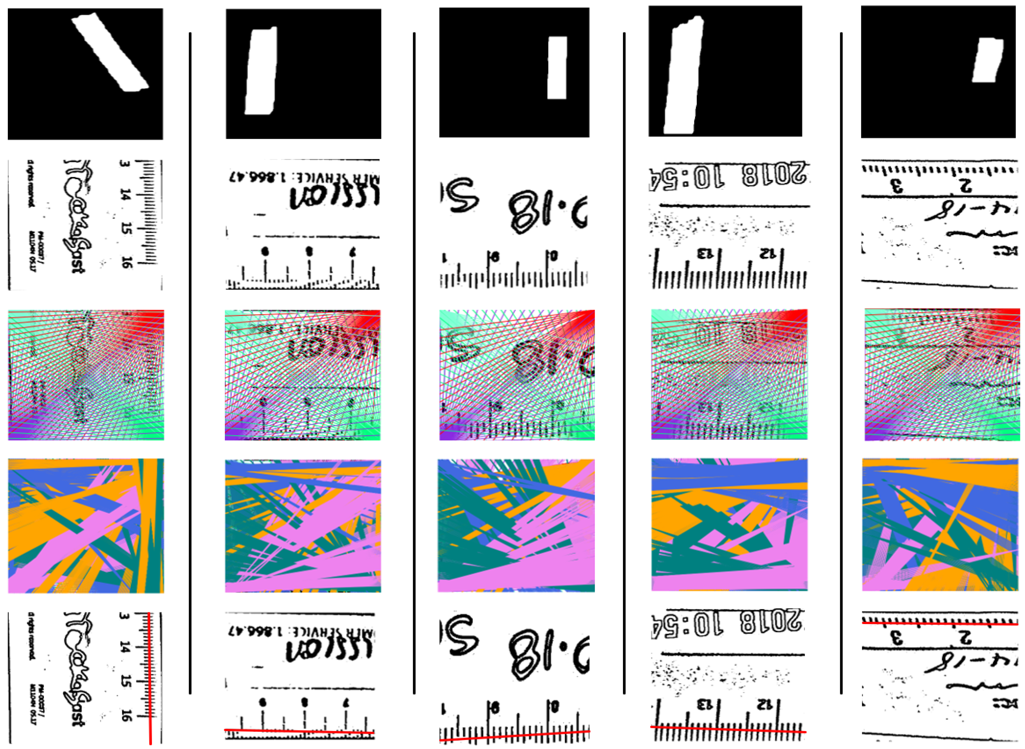
With the current system the results with our segmentation of the ruler and the results of the heuristic method are separated as depicted in Figure 6. Since MRCNN is well cited and popular for its results, we include the results of our adaptation of the model and technique for images containing rulers but only for detection.

3.1. Segmentation Results

The result of MRCNN, specifically the instance detection, is given in terms of the object detection confidence. In our experiment we took 30 images containing either a white, green, or brown graduated ruler in the shot. The rulers used varied in shape and size. The rulers used had: just metric graduations, just imperial graduations, and both metric/imperial graduations on the same ruler. In metric, rulers had lengths of 5, 15, and 30 cm. The background of the images were largely unique to each image. With Mask R-CNN we were able to achieve an average confidence score of 99.97%. In terms of our system this means we are almost certainly guaranteed a bounding box to start calibrating the image. This is because a bounding box is only generated by MRCNN when there is a detection score; however, if the detection score is too low the background area will be an issue for our system as mentioned in Section 2.1.
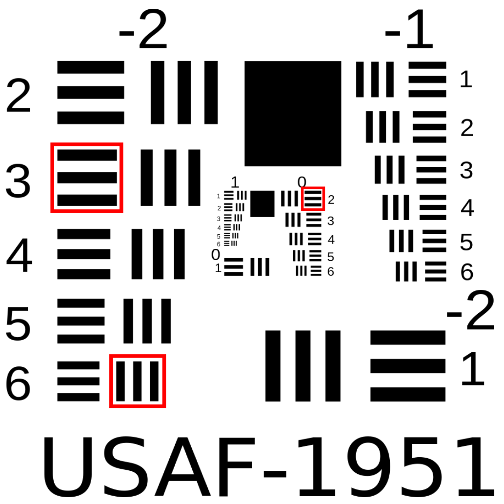
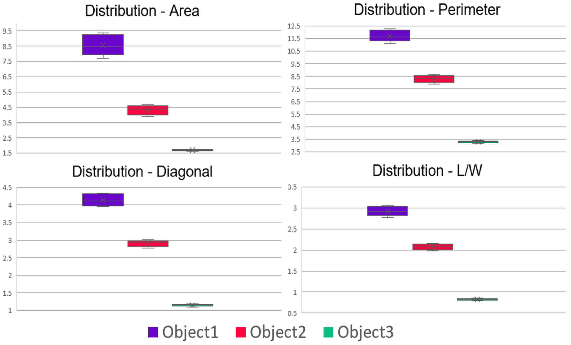
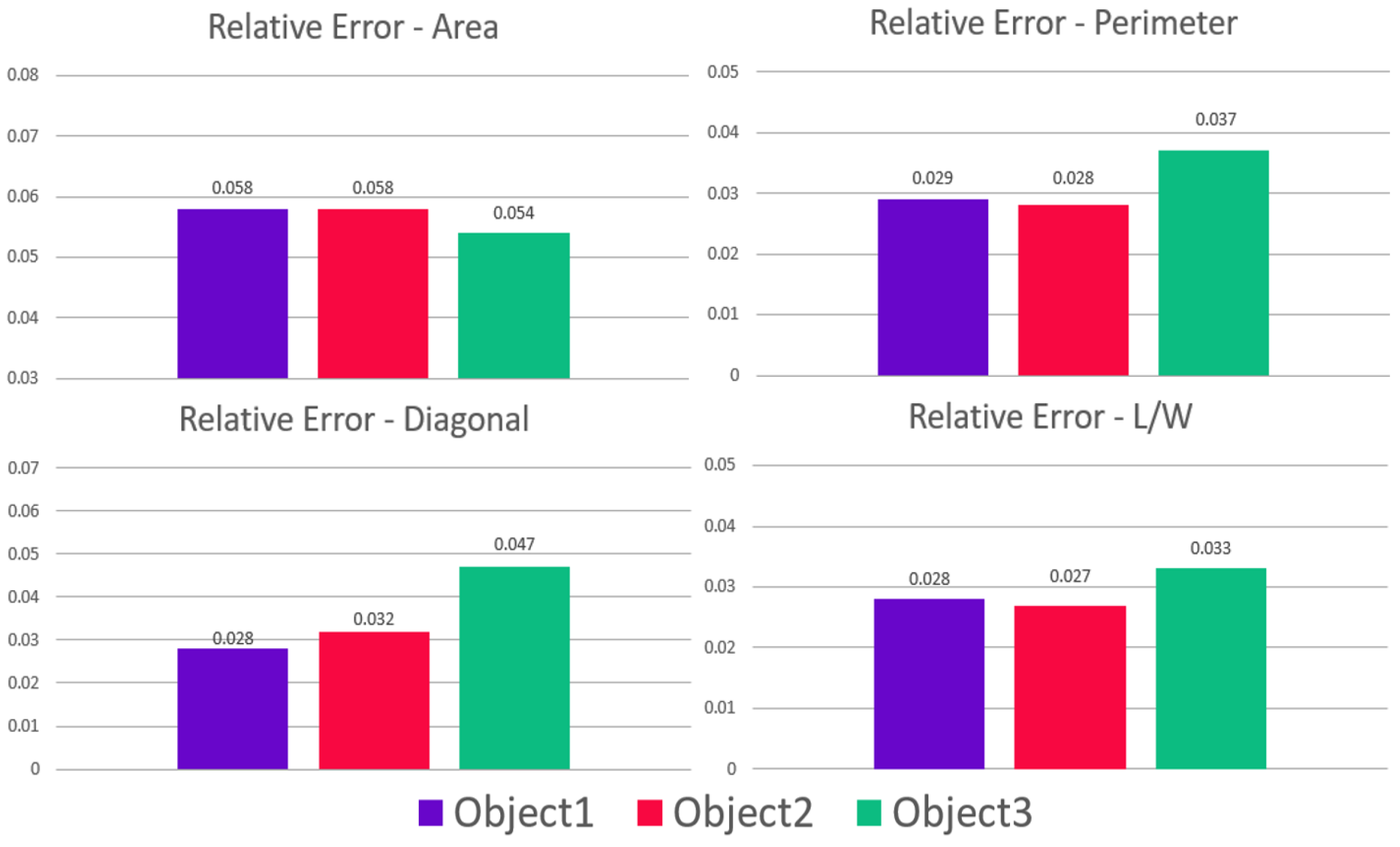
The heuristic method was tested on a printed USAF-1951 target in Figure 7 where three reference objects of different sizes, surrounded by red boxes were selected. The objects considered were measured from the first black stripe to the third black stripe for area, perimeter, diagonal, and length/width. Each photograph taken of the objects was done with a ruler in the shot. Several shots were taken at different heights while the rest were taken at roughly the same height. This was done to test the robustness of the search in terms of variance in the measure. We found that a picture taken very close to the reference objects induced more error. This is because we do not measure at the sub-pixel level in our method and the system is rounding off error to the nearest pixel. The metric measurements for each object are presented in Table 1. Noting the measurements for Length/Width as an average of two measured sides. Area was calculated as the square of the average for the Length/Width. Ten pictures at 4032 × 3024 pixels resolution were taken of the target using an iPhone X’s 12MP f/1.8 4 mm camera. Each object was measured in pixels after the photo was taken using the “Measure” tool in ImageJ2 [40]. The measurements for each of the objects in each of the ten pictures is shown in Figure 8. The absolute error of these measurements are presented in Figure 9.

3.2. Heuristic Search Calibration Results

We performed real measurements for the Area, L/W, Diagonal, and Perimeter, both in metrics and in pixels. We expected the error to be squared in the area measurements and have included it in our results for completeness. We found that on average the measurement for calibrating the test image was 9 pixels/millimeter. Our calibrated results include the images taken at different heights are included in Figure 8 and Figure 9. From the 24 of the 30 measurements for length and width our proposed calibration method measured within 1 mm of error with the remaining 6 having less than 2 mm of error. The average of the 10 measurements obtained for objects 1, 2, and 3 are 2.92 cm, 2.08 cm, and 0.82 cm, respectively. Figure 9 shows the relative error for L/W, Diagonal, and Perimeter measurements was less than 5 % with the relative error for Area less than 6 % . We found that the system performed slightly better on Object 1 and 2 than it did for Object 3. As Object 3 is the smallest, with a length of 8 mm, this can be attributed to our measurements being done at the pixel level.
We believe these results are meaningful as the general error in any systematic measuring device is plus or minus the minimum unit of measure, in our tests this was plus or minus 1 mm. In our tests, 87 % of the time, results were well within this margin of error and we believe the measurements with 2 mm of error could partially be attributed to our error in measurement using the ImageJ2 “Measure” tool. In addition, as we have mentioned several times before, the system only samples the image at a pixel level, which could be cause for the additional millimeter of error.

4. Conclusions

In this paper we proposed a new system for automated calibration of images when a ruler is present in the scene. This is done by extracting the ruler and measuring its graduations as a spatial frequency. This system produces accurate and reproducible results, removing the tedious manual labor to perform metrological tasks. The robust and extensible OpenCV packages allowed us to formulate and execute image transforms that were necessary to move through the pipeline of data extraction. Aside from OpenCV we created the initial/deep search from scratch instead of applying more pre-built methods. This allowed us to fine tune the search and consider broader scenarios. We used Mask R-CNN to produce satisfactory ruler masks, with this technique we were able to remove the majority of uncertainty when handling rulers with widely varying backgrounds. Our system samples the image data at the pixel level which was mainly done to broaden the capabilities that the system could work on, namely different resolutions. When sampling at a sub-pixel level, assumptions about recording devices’ parameters need to be made and manually input to the system. In order to overcome this difficulty, we trained Mask R-CNN to do semantic segmentation on rulers normalizing the segmented masks.
In addition to Hough line transform or Fourier transforms to extract the graduations on a ruler, limiting the ability to perform sub-pixel measurements, we iteratively reduce the search space of the graduations and perform a search for spatial frequencies corresponding to the ruler’s graduation. This provides reproducable results on a wide variety of images. From end to end the extracted pixel to metric ratios or DPI/DPM can be found on average in 5.6 s.
In the future we look forward to optimizing the system, further reducing the search time and space on the deep search stage. We are currently working on implementing several methods to decrease the number of search candidates that would most likely not be in the region of the ruler’s graduation. The system today stores many search results in case the heuristic model point backwards, this ultimately leads to still having many empty/wasted searches. Additionally, we look forward to finding a solution for halting the system early, potentially prior to performing either the initial or deep search, skipping the deep search when possible. This would lead to faster results from our system.

Author Contributions

Conceptualization: D.S.-S. and A.S.E.; methodology: M.T.; validation: M.T., D.S.-S. and A.S.E.; project administration: D.S.-S. and A.S.E.; formal analysis M.T. and D.S.-S.; software: M.T.; writing—original draft, M.T.; writing—review and editing, M.T., D.S.-S., and A.S.E. All authors have read and agreed to the published version of the manuscript.

Funding

This research received no external funding.

Conflicts of Interest

The authors declare no conflict of interest.

Code Availability

The code that support the findings of this study are available from the corresponding author upon justified email request.

References

  1. Yan, J.; Downey, A.; Cancelli, A.; Laflamme, S.; Chen, A.; Li, J.; Ubertini, F. Concrete crack detection and monitoring using a capacitive dense sensor array. Sensors 2019, 19, 1843. [Google Scholar] [CrossRef] [PubMed] [Green Version]
  2. Herrera-Téllez, V.I.; Cruz-Olmedo, A.K.; Plasencia, J.; Gavilanes-Ruíz, M.; Arce-Cervantes, O.; Hernández-León, S.; Saucedo-García, M. The protective effect of Trichoderma asperellum on tomato plants against Fusarium oxysporum and Botrytis cinerea diseases involves inhibition of reactive oxygen species production. Int. J. Mol. Sci. 2019, 20, 2007. [Google Scholar] [CrossRef] [PubMed] [Green Version]
  3. Kekonen, A.; Bergelin, M.; Johansson, M.; Kumar Joon, N.; Bobacka, J.; Viik, J. Bioimpedance Sensor Array for Long-Term Monitoring of Wound Healing from Beneath the Primary Dressings and Controlled Formation of H2O2 Using Low-Intensity Direct Current. Sensors 2019, 19, 2505. [Google Scholar] [CrossRef] [PubMed] [Green Version]
  4. Nirenberg, M.S.; Ansert, E.; Krishan, K.; Kanchan, T. Two-dimensional linear analysis of dynamic bare footprints: A comparison of measurement techniques. Sci. Justice 2019, 59, 552–557. [Google Scholar] [CrossRef]
  5. Ortiz-Coder, P.; Sánchez-Ríos, A. A Self-Assembly Portable Mobile Mapping System for Archeological Reconstruction Based on VSLAM-Photogrammetric Algorithm. Sensors 2019, 19, 3952. [Google Scholar]
  6. Rodriguez-Padilla, I.; Castelle, B.; Marieu, V.; Morichon, D. A Simple and Efficient Image Stabilization Method for Coastal Monitoring Video Systems. Remote Sens. 2020, 12, 70. [Google Scholar] [CrossRef] [Green Version]
  7. Agapiou, A. Optimal Spatial Resolution for the Detection and Discrimination of Archaeological Proxies in Areas with Spectral Heterogeneity. Remote Sens. 2020, 12, 136. [Google Scholar] [CrossRef] [Green Version]
  8. Bishop, C.M. Pattern Recognition and Machine Learning; Springer: Berlin/Heidelberg, Germany, 2006. [Google Scholar]
  9. Long, J.; Shelhamer, E.; Darrell, T. Fully convolutional networks for semantic segmentation. In Proceedings of the IEEE Conference on Computer Vision and Pattern Recognition, Boston, MA, USA, 7–12 June 2015; pp. 3431–3440. [Google Scholar]
  10. Calatroni, L.; van Gennip, Y.; Schönlieb, C.B.; Rowland, H.M.; Flenner, A. Graph clustering, variational image segmentation methods and Hough transform scale detection for object measurement in images. J. Math. Imaging Vis. 2017, 57, 269–291. [Google Scholar] [CrossRef] [Green Version]
  11. Bhalerao, A.; Reynolds, G. Ruler detection for autoscaling forensic images. Int. J. Digit. Crime Forensics (IJDCF) 2014, 6, 9–27. [Google Scholar] [CrossRef] [Green Version]
  12. Belay, B.; Habtegebrial, T.; Meshesha, M.; Liwicki, M.; Belay, G.; Stricker, D. Amharic OCR: An End-to-End Learning. Appl. Sci. 2020, 10, 1117. [Google Scholar] [CrossRef] [Green Version]
  13. Balado, J.; Martínez-Sánchez, J.; Arias, P.; Novo, A. Road environment semantic segmentation with deep learning from MLS point cloud data. Sensors 2019, 19, 3466. [Google Scholar] [CrossRef] [Green Version]
  14. Velazquez-Pupo, R.; Sierra-Romero, A.; Torres-Roman, D.; Shkvarko, Y.V.; Santiago-Paz, J.; Gómez-Gutiérrez, D.; Robles-Valdez, D.; Hermosillo-Reynoso, F.; Romero-Delgado, M. Vehicle detection with occlusion handling, tracking, and OC-SVM classification: A high performance vision-based system. Sensors 2018, 18, 374. [Google Scholar] [CrossRef] [Green Version]
  15. Yang, F.; Kale, A.; Bubnov, Y.; Stein, L.; Wang, Q.; Kiapour, H.; Piramuthu, R. Visual search at ebay. In Proceedings of the 23rd ACM SIGKDD International Conference on Knowledge Discovery and Data Mining, Halifax, NS, Canada, 13–17 August 2017; pp. 2101–2110. [Google Scholar]
  16. Zhu, Z.; Yin, H.; Chai, Y.; Li, Y.; Qi, G. A novel multi-modality image fusion method based on image decomposition and sparse representation. Inf. Sci. 2018, 432, 516–529. [Google Scholar] [CrossRef]
  17. Papageorgiou, C.P.; Oren, M.; Poggio, T. A general framework for object detection. In Proceedings of the Sixth International Conference on Computer Vision (IEEE Cat. No. 98CH36271), Bombay, India, 7 January 1998; pp. 555–562. [Google Scholar]
  18. Viola, P.; Jones, M. Robust real-time object detection. Int. J. Comput. Vis. 2001, 4, 4. [Google Scholar]
  19. Girshick, R.; Donahue, J.; Darrell, T.; Malik, J. Region-based convolutional networks for accurate object detection and segmentation. IEEE Trans. Pattern Anal. Mach. Intell. 2015, 38, 142–158. [Google Scholar] [CrossRef]
  20. Redmon, J.; Divvala, S.; Girshick, R.; Farhadi, A. You only look once: Unified, real-time object detection. In Proceedings of the IEEE Conference on Computer Vision and Pattern Recognition, Las Vegas, NV, USA, 27–30 June 2016; pp. 779–788. [Google Scholar]
  21. Shafiee, M.J.; Chywl, B.; Li, F.; Wong, A. Fast YOLO: A fast you only look once system for real-time embedded object detection in video. arXiv 2017, arXiv:1709.05943. [Google Scholar] [CrossRef]
  22. Liu, W.; Anguelov, D.; Erhan, D.; Szegedy, C.; Reed, S.; Fu, C.Y.; Berg, A.C. Ssd: Single shot multibox detector. In Proceedings of the European Conference on Computer Vision, Amsterdam, The Netherlands, 11–14 October 2016; pp. 21–37. [Google Scholar]
  23. Zoph, B.; Le, Q.V. Neural architecture search with reinforcement learning. arXiv 2016, arXiv:1611.01578. [Google Scholar]
  24. Dai, J.; Li, Y.; He, K.; Sun, J. R-fcn: Object detection via region-based fully convolutional networks. In Proceedings of the Advances in Neural Information Processing Systems, Barcelona, Spain, 5–10 December 2016; pp. 379–387. [Google Scholar]
  25. Girshick, R. Fast r-cnn. In Proceedings of the IEEE Conference on Computer Vision and Pattern Recognition, Boston, MA, USA, 7–12 June 2015; pp. 1440–1448. [Google Scholar]
  26. Ren, S.; He, K.; Girshick, R.; Sun, J. Faster r-cnn: Towards real-time object detection with region proposal networks. In Proceedings of the Advances in Neural Information Processing Systems, Barcelona, Spain, 5–10 December 2016; pp. 91–99. [Google Scholar]
  27. He, K.; Gkioxari, G.; Dollár, P.; Girshick, R. Mask r-cnn. In Proceedings of the IEEE International Conference on Computer Vision, Venice, Italy, 22–29 October 2017; pp. 2961–2969. [Google Scholar]
  28. Ammirato, P.; Berg, A.C. A Mask-RCNN Baseline for Probabilistic Object Detection. arXiv 2019, arXiv:1908.03621. [Google Scholar]
  29. Yu, Y.; Zhang, K.; Yang, L.; Zhang, D. Fruit detection for strawberry harvesting robot in non-structural environment based on Mask-RCNN. Comput. Electron. Agric. 2019, 163, 104846. [Google Scholar] [CrossRef]
  30. Haralick, R.M.; Shapiro, L.G. Image segmentation techniques. Comput. Vis. Graph. Image Process. 1985, 29, 100–132. [Google Scholar] [CrossRef]
  31. Hong, J.; Cho, B.; Hong, Y.W.; Byun, H. Contextual Action Cues from Camera Sensor for Multi-Stream Action Recognition. Sensors 2019, 19, 1382. [Google Scholar] [CrossRef] [Green Version]
  32. Jiang, H.; Lu, N. Multi-scale residual convolutional neural network for haze removal of remote sensing images. Remote Sens. 2018, 10, 945. [Google Scholar] [CrossRef] [Green Version]
  33. Qiu, R.; Yang, C.; Moghimi, A.; Zhang, M.; Steffenson, B.J.; Hirsch, C.D. Detection of Fusarium Head Blight in Wheat Using a Deep Neural Network and Color Imaging. Remote Sens. 2019, 11, 2658. [Google Scholar] [CrossRef] [Green Version]
  34. Wang, E.K.; Zhang, X.; Pan, L.; Cheng, C.; Dimitrakopoulou-Strauss, A.; Li, Y.; Zhe, N. Multi-path dilated residual network for nuclei segmentation and detection. Cells 2019, 8, 499. [Google Scholar] [CrossRef] [Green Version]
  35. Lin, T.Y.; Dollár, P.; Girshick, R.; He, K.; Hariharan, B.; Belongie, S. Feature pyramid networks for object detection. In Proceedings of the IEEE International Conference on Computer Vision, Venice, Italy, 22–29 October 2017; pp. 2117–2125. [Google Scholar]
  36. Bradski, G. The OpenCV Library. Dr. Dobb’S J. Softw. Tools 2000, 25, 120–125. [Google Scholar]
  37. Zemmour, E.; Kurtser, P.; Edan, Y. Automatic parameter tuning for adaptive thresholding in fruit detection. Sensors 2019, 19, 2130. [Google Scholar] [CrossRef] [Green Version]
  38. Zhang, T.; Huang, Z.; You, W.; Lin, J.; Tang, X.; Huang, H. An Autonomous Fruit and Vegetable Harvester with a Low-Cost Gripper Using a 3D Sensor. Sensors 2020, 20, 93. [Google Scholar] [CrossRef] [Green Version]
  39. Zhang, J.; Guo, Z.; Jiao, T.; Wang, M. Defect Detection of Aluminum Alloy Wheels in Radiography Images Using Adaptive Threshold and Morphological Reconstruction. Appl. Sci. 2018, 8, 2365. [Google Scholar] [CrossRef] [Green Version]
  40. Rueden, C.T.; Schindelin, J.; Hiner, M.C.; DeZonia, B.E.; Walter, A.E.; Arena, E.T.; Eliceiri, K.W. ImageJ2: ImageJ for the next generation of scientific image data. BMC Bioinform. 2017, 18, 529. [Google Scholar] [CrossRef]
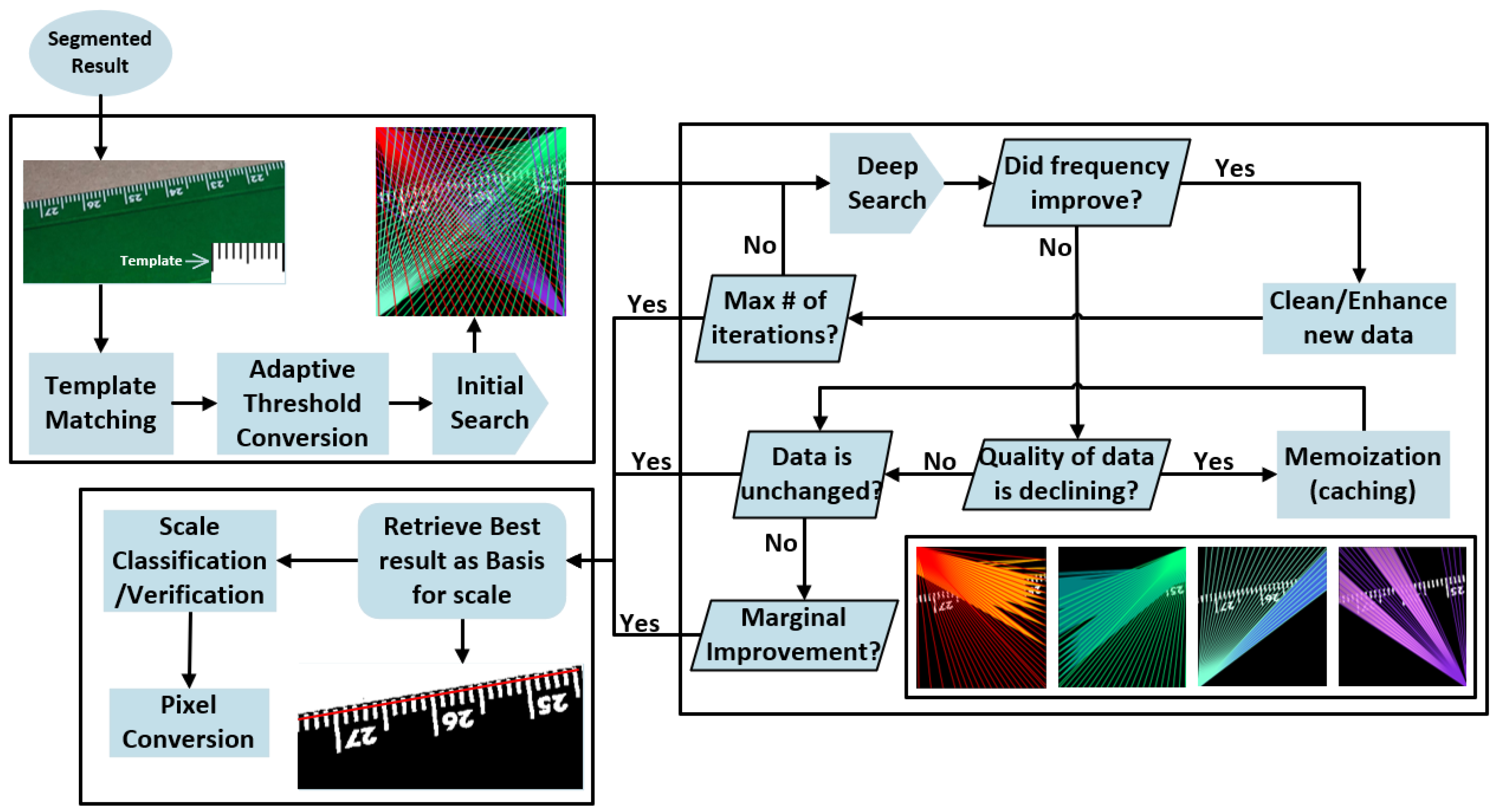
Figure 1. High Level Architecture proposed heuristic method for scale calibration (best seen in color).
Information 11 00259 g001
Figure 2. (Overview Procedure) Integration of Mask Region proposal based Convolutional Neural Network (R-CNN) output with scale calibration system for calibrating an image.
Information 11 00259 g002
Figure 3. (Deep Search Rendering) (a) All searches collectively. Note the crisscrossing at the top of the image where the density shows the search optimization. (b) Each search separated by the corner where the search started. In the top left, the red lines correspond to the initial search. (c) A zoomed in piece of each search where a set of ticks are located (best seen in color).
Information 11 00259 g003
Figure 4. (Final Spatial Frequency) On top is the line used to measure M f . Below is the line graduation distribution in pixels.
Information 11 00259 g004
Figure 5. (Scale Search and Results) Left are the search lines. Right displays both the line and the distribution of 5 M f and 10 M f .
Information 11 00259 g005
Figure 6. Database test results on five images. From top to bottom: Mask R-CNN (MRCNN) output, template match, initial search, deep search, and final calibrating line (best seen in color).
Information 11 00259 g006
Figure 7. (Test Target) The printed target from the United States Air Force used for testing and measuring the heuristic calibration method.
Information 11 00259 g007
Figure 8. Distribution of measurements performed using proposed heuristic calibration method. Object 1 is the largest object from Figure 7, Object 2 is the second largest object, and Object 3 is the smallest object.
Information 11 00259 g008
Figure 9. Absolute error for each of the measurements tested by the proposed heuristic calibration method.
Information 11 00259 g009
Table 1. The manual measurements of the printed target using a metric ruler. Object 1 is the largest object from Figure 7, Object 2 is the second largest object, and Object 3 is the smallest object.
Measurement (Scale)Object 1Object 2Object 3
Area (cm 2 )8.414.411.6
Perimeter (cm)11.68.43.2
Diagonal (cm)4.13.01.1
Length × Width (cm)2.9 × 2.92.1 × 2.10.8 × 0.8