A Noise Study of the PSW Signature Family: Patching DRS with Uniform Distribution ^†

Abstract

At PKC 2008, Plantard et al. published a theoretical framework for a lattice-based signature scheme, namely Plantard–Susilo–Win (PSW). Recently, after ten years, a new signature scheme dubbed the Diagonal Reduction Signature (DRS) scheme was presented in the National Institute of Standards and Technology (NIST) PQC Standardization as a concrete instantiation of the initial work. Unfortunately, the initial submission was challenged by Yu and Ducas using the structure that is present on the secret key noise. In this paper, we are proposing a new method to generate random noise in the DRS scheme to eliminate the aforementioned attack, and all subsequent potential variants. This involves sampling vectors from the n-dimensional ball with uniform distribution. We also give insight on some underlying properties which affects both security and efficiency on the PSW type schemes and beyond, and hopefully increase the understanding on this family of lattices.

1. Introduction

The popularity of post-quantum cryptography has increased significantly after the formal announcement by the NIST to move away from classical cryptography [1]. This is due to the potential threat that will be brought by the upcoming large-scale quantum computers, which theoretically break the underlying traditional hard problem by using Shor’s algorithm [2]. Post-quantum cryptography, in short, is the conception and analysis of cryptographic tools that are practically available to classical computers but quantum-safe (i.e., safe against quantum computers).

To do so, one usually uses a mathematical structure in which computational problems are perceived to be hard. There are currently three big families of mathematical structures in post-quantum cryptology, namely code-based cryptography, multivariate cryptography, and lattice-based cryptography. Smaller families do exist: hash-based functions, isogenies, etc. This work, however, primarily concerns with lattice-based cryptography. First introduced by Minkowski in a pioneering work [3] to solve various number problems, lattices have the advantage to often base their security on worst-case assumptions [4] rather than the average case, and to be highly parallelizable and algorithmically simple enough to compete with traditional schemes in terms of computing speed. Inspired by this, Goldreich, Goldwasser and Halevi [5] proposed an efficient way to use lattices to build a public-key encryption scheme, namely the Goldreich-Goldwasser-Halevi (GGH) scheme. The initial iteration of GGH has been broken using lattice reduction techniques [6], however, the central idea remains viable and it has enabled a wide array of applications and improvements, such as using tensor products [7], Hermite Normal Form (HNF) [8], polynomial representations [9], rotations [10], and the most popular one being Learning With Errors (LWE) [11] or its variants. One particular class of lattices enjoy a remarkable reputation: q-ary lattices. This family benefits from the worst-case hardness reduction proof from Ajtai [4] and Regev [11] using two dual problems: Short Integer Solution (SIS) and LWE. Lately, Gama, Izabachene, Nguyen and Xie have been shown that most lattices in general benefit from this specific hardness reduction [12]. However, as this was relatively new, constructing lattice-based schemes outside of the q-ary family is still unpopular.

More recently, the NIST attempt at standardizing post-quantum cryptography [13] received a lot of interest from the community and the vast majority of the lattice-based submissions for “Round 1” are actually based on LWE/SIS or their variants [13]. One of the few lattice-based submissions outside of the q-ary family is the DRS Scheme [14], which uses a diagonal dominant matrix that can be seen as a sum between a diagonal matrix with very big coefficients and a random matrix with low coefficients. DRS was based on the original PSW framework from [15], however, the original paper had mostly a theoretical interest and did not provide an explicit way to construct the random matrix with low values, rather than merely stating conditions on norm bounds it should respect for the signature scheme to be proven functioning. The NIST submission, however, provides a more straight-forward way to generate the noise, using another proof and condition to ensure the functionality of the scheme. This new way to generate the noise, however, is shown to be insecure: Soon after DRS was made public, Yu and Ducas used machine learning techniques to severely reduce the security parameters [16]. While according to Ducas’ comments on the NIST forum [13], the attack was not devastating as it still seems asymptotically secure, however, its concrete security was significantly decreased. On the same work, Yu and Ducas also provided several suggestions in order to fix those issues and one of those comments suggested using a statistical analysis. Another more recent attack from Li, Liu, Nitaj and Pan [17] on a randomized version of the initial scheme proposed by Plantard, Susilo and Win [15] can also be indirectly considered an attack to the DRS scheme, although this attack does not seem as important as Yu and Ducas’s one.

In the following work, we do follow some of those suggestions and we aim to provide a new noise generation method to eliminate the aforementioned attack and restore some of the DRS’ concrete security. We will present some statistical heuristics and remove some of the structure that allow the initial DRS scheme to be attacked and discuss open questions and alternatives.

Our Contribution and Paper Organization

The rest of the paper is organized as follows. We first present some relevant background on lattice theory and re-introduce the DRS scheme from Plantard et al. Subsequently, we will comment on the attack of Li, Liu, Nitaj and Pan [17] and explain why it is not applicable. Then we discuss the weakness found by Yu and Ducas and our idea to correct this. We finally present the detail algorithms about our security patch, discuss the relative hardness of the patch, alternative approaches and raise some open questions.

2. Background

In this section, we briefly recall the basics of lattice theory.

2.1. Lattice Theory

Definition 1

(Integral lattice). We call lattice a discrete subgroup of ${\mathbb{R}}^n$ where n is a positive integer. We say a lattice is an integral lattice when it is a subgroup of ${\mathbb{Z}}^n$. A basis of the lattice is a basis as a $\mathbb{Z}-module$. If M is a matrix, we define $\mathcal{L}\left(M\right)$ the lattice generated by the rows of M.

In this work we only consider full-rank integer lattices, i.e., such that their basis can be repcresented by a $n\times n$ non-singular integer matrix.

Theorem 1

(Determinant). For any lattice $\mathcal{L}$, there exists a real value we call determinant, denoted $det\left(\mathcal{L}\right)$, such that for any basis B, $det\left(\mathcal{L}\right)=\sqrt{det\left(B{B}^T\right)}$.

The literature sometimes call $det\left(\mathcal{L}\right)$ as the volume of $\mathcal{L}$ [3]. In the full-rank case, $det\left(\mathcal{L}\right)=\sqrt{det\left(B\right)}$ and we say B is non-singular (or invertible) when $det\left(B\right)\ne 0$.

We note that the definition is similar to the one which can be found in fundamental mathematics books [18] for diagonal dominant matrices. We will just adapt the lattice to its diagonal dominant basis.

Definition 2

(Minima). We note ${\lambda }_i\left(\mathcal{L}\right)$ the $i-$th minimum of a lattice $\mathcal{L}$. It is the radius of the smallest zero-centered ball containing at least i linearly independant elements of $\mathcal{L}$.

Definition 3

(Lattice gap). We note ${\delta }_i\left(\mathcal{L}\right)$ the ratio $\frac{{\lambda }_{i+1}\left(\mathcal{L}\right)}{{\lambda }_i\left(\mathcal{L}\right)}$ and call that a lattice gap. When mentioned without index and called “the” gap, the index is implied to be $i=1$.

In practice, only the case $i=1$ is used, but other values are sometimes useful to consider [19]. We also define the “root lattice gap”, i.e., elevated to the power $\frac{1}{n}$ where n is the dimension of the lattice.

Definition 4

(Diagonal Dominant Lattices). We say a lattice is a diagonally dominant type lattice (of dimension n) if it admits a diagonal dominant matrix as a basis B as in [18], i.e.,

$$\forall i\in [1,n],B_{i,i}\ge {\sum }_{j=1,i\ne j}^n\left|B_{i,j}\right|$$

We can also see a diagonally dominant matrix B as a sum $B=D+R$ where D is diagonal and $D_{i,i}>{\parallel R_i\parallel }_1$. To avoid conflicting notations between the diagonal matrix and the diagonal coefficient, we will denote from now on $D_{Id}$ the product of the integer D by the canonical basis $Id$. We might also denote $D_g$ a diagonal matrix which diagonal coefficients might not all be equals. In our scheme, we use a diagonal dominant lattice as our secret key, and will refer to it as our “reduction matrix” (as we use this basis to “reduce” our vectors).

Definition 5

(Vector Norms). Let F be a subfield of $\mathbb{C}$, V a vector space over $F^k$, and p a positive integer or ∞. We call $l_p$ norm over V the norm:

• $\forall x\in {V,\parallel x\parallel }_p=\sqrt[p]{{\sum }_{i=1}^k{\left|x_i\right|}^p}$
• $\forall x\in {V,\parallel x\parallel }_{\infty }={max}_{i\in [1,k]}\left|x_i\right|$

$l_1$ and $l_2$ are commonly used and are often called taxicab norm and Euclidean norm, respectively. We note that we also define the maximum matrix norm as the biggest value among the sums of the absolute values in a single column.

The norm that was used by Plantard et al. for their signature validity is the maximum norm. However, as far as the security heuristics are concerned the Euclidean norm ($l_2$) is used, and as far as the reduction termination proof is concerned the taxicab norm ($l_1$) is used.

Definition 6

(Matrix Norms). Let A be a square matrix in ${\mathbb{C}}^{n,n}$. A matrix norm denoted as $\parallel A\parallel$ is said to be consistent to a vector norm $\parallel .\parallel$, if we have $\parallel A\parallel =sup\{\parallel xA\parallel ,x\in {\mathbb{C}}^n,\parallel x\parallel =1\}$.

Matrix norms were an useful analytic tools in [15], and can also be used to simplify notations.

Definition 7

(Trace of a matrix). Let A be a square matrix in ${\mathbb{C}}^{n,n}$. We say $tr\left(A\right)={\sum }_{i=1}^n{A}_{i,i}$ is the trace of A.

2.2. Lattice Problems

The most famous problems on lattice are the Shortest Vector Problem (SVP) and the Closest Vector Problem (CVP). We tend to approximatively solve the CVP by solving heuristically SVP in an expanded lattice [5].

Definition 8

(Closest Vector Problem (CVP)). Given a basis B of a lattice $\mathcal{L}$ of dimension n and $t\in {\mathbb{R}}^n$, find $y\in \mathcal{L}$ such that $\forall y_2\in \mathcal{L},\parallel t-y\parallel \le \parallel t-y_2\parallel$.

Definition 9

(Shortest Vector Problem (SVP)). Given a basis B of a lattice $\mathcal{L}$ of dimension n, find $y\in \mathcal{L}$ such that $\parallel y\parallel ={\lambda }_1\left(B\right)$.

In cryptography, we rely on the “easier” versions of those problems:

Definition 10

($\gamma$-unique Shortest Vector Problem (${uSVP}_{\gamma }$)). Given a basis of a lattice $\mathcal{L}$ with its lattice gap $\delta >1$, solve SVP.

Since ${\lambda }_1\left(\mathcal{L}\right)$ is also hard to determine (it is indeed another lattice problem we do not state here), measuring the efficiency of an algorithm is another challenge by itself. Therefore, to measure algorithm efficiency we must be able to define a problem with easily computable parameters, which is where the Hermite factor is originated from:

Definition 11

($\gamma$-Hermite Shortest Vector Problem (${HSVP}_{\gamma }$)). Given a basis B of a lattice $\mathcal{L}$ of dimension n and a factor γ we call Hermite Factor, find $y\in \mathcal{L}$ such that $\parallel y\parallel \le \gamma det{\left(\mathcal{L}\right)}^{1/n}$.

Some cryptosystems are based on worst-case hardness on ${uSVP}_{\gamma }$ with polynomial gap as [20] and [11]. The practical hardness of ${uSVP}_{\gamma }$ depends on its gap compared to a fraction of the Hermite factor, where the constant in front of the factor depends of the lattice and the algorithm used [21]. There exists an attack that was specifically built to exploit high gaps [22].

Definition 12

($\gamma$-Bounded Distance Decoding (${BDD}_{\gamma }$)). Given a basis B of a lattice $\mathcal{L}$, a point x and a approximation factor γ ensuring $d(x,\mathcal{L})<\gamma {\lambda }_1\left(B\right)$ find the lattice vector $v\in \mathcal{L}$ closest to x. When $\gamma =1/2$, we can omit γ and note the problem Bounded Distance Decoding (BDD).

It has been proved that ${BDD}_{1/\left(2\gamma \right)}$ reduces itself to ${uSVP}_{\gamma }$ in polynomial time and the same goes from ${uSVP}_{\gamma }$ to ${BDD}_{1/\gamma }$ when $\gamma$ is polynomially bounded by n [23], in cryptography the gap is polynomial the target point x must be polynomially bounded therefore, solving one or the other is relatively the same in our case. To solve those problems, we usually use an embedding technique that extends a basis matrix by one column and one row vector that are full of zeroes except for one position where the value is set to 1 at the intersection of those newly added spaces, and then apply lattice reduction techniques on these. As far as their signature scheme is concerned, the ${GDD}_{\gamma }$ is more relevant:

Definition 13

($\gamma$-Guaranteed Distance Decoding (${GDD}_{\gamma }$)). Given a basis B of a lattice $\mathcal{L}$, and a bound γ, for any point x find a lattice vector $v\in \mathcal{L}$ such that $\parallel x-v\parallel <\gamma$.

As far as recovering a secret key is concerned, usually the problem reduces to SVP. However, if a whole short basis is concerned, then the following problem becomes relevant:

Definition 14

(Shortest Basis Problem (SBP)). Given a basis of a lattice $\mathcal{L}$ of rank n, find a basis $y_1,\dots ,y_n\in \mathcal{L}$ such that

$$ma{x}_i\parallel y_i\parallel \le min\{ma{x}_j\parallel a_j\parallel |\{a_1,\dots ,a_n\}\mathit{is}a\mathit{basis}\mathit{of}\mathcal{L}\}.$$

3. The Theoretical Framework of Plantard–Susilo–Win

3.1. Before PSW: Lattices for Number Representation

Before we present PSW, we will briefly give some hindsight about “number systems”, i.e., ways to represent a number. The reason might not be apparent, but we hope a few examples will actually help understand the core ideas behind PSW and DRS. We are not going to talk about Residue Number System (RNS) or the Chinese Remainder Theorem (CRT) which are famous number systems, but clearly irrelevant for what we present in this paper. Instead, we are going to talk about the very basic representations of numbers.

Suppose we want to represent a number x in base k, such that $x<k^n$. Then the number has the unique following representation:

$$x=x_0+x_{1}k+x_2{k}^2+\dots x_n{k}^n\mathrm{such}\mathrm{that}\forall i,x_i\in [0,k-1]$$

Basically, the role of k is mostly to determine the number of symbols used, and the positions $1,k,k^2,\dots ,k^n$ are written from increasing power from left to right for a simple representation when writing the number

$$x=“x_0{x}_{1}k{x}_2\dots x_n^{”}$$

Using $k=10$ gives us the arabic numerotation most of us use today in science. but then, what if we decide to strip the condition “$\forall i,x_i\in [0,k-1]$”? The representation is then obviously not unique anymore:

$$x=(x-\lfloor x/k\rfloor )+\lfloor x/k\rfloor k=(x-(\lfloor (x-\lfloor x/k^2\rfloor )/k\rfloor +\lfloor x/k^2\rfloor k^2))+\lfloor (x-\lfloor x/k^2\rfloor )/k\rfloor +\lfloor x/k^2\rfloor k^2=\dots$$

Most informed people would see here a reversing of the table Euclidean division. However we are choosing another representation: we can also represent this phenomenon by a vector. In the following example we reverse the order, putting the highest degree on the left:

$$1851\simeq [1,8,5,1]$$

$$1851=1\times {10}^3+0\times {10}^2+85\times {10}^1+1\times {10}^0\simeq [1,0,85,1]$$

$$1851=0\times {10}^3+18\times {10}^2+0\times {10}^1+51\times {10}^0\simeq [0,18,0,51]$$

We can see here, that all numbers are obtained by linear combinations by the vectors of the following matrices:

$B_{10}=\left[\begin{array}{cccc}-1& 10& 0& 0\\ 0& -1& 10& 0\\ 0& 0& -1& 10\end{array}\right]$ and in base k would give $B_k=\left[\begin{array}{cccc}-1& k& 0& 0\\ 0& -1& k& 0\\ 0& 0& -1& k\end{array}\right]$

$[1,8,5,1]\equiv [1,0,85,1]\equiv [0,18,0,51]mod\mathcal{L}\left(B_{10}\right)$

To decompose vectors in the unique representation we use in “everyday life”, we would reduce successively the i-th coefficient to the maximum with the i-th vector, from the first to the last, which is, rightfully so, the equivalent of a Euclidean division. Here the reduction works intuitively as we are subtracting some large multiple of k in a position to add a small multiple of 1 in another. What now if we decide to use number systems that are not the “number-system” lattice we showcased? Instead of classical Euclidean division we could use some form of approximation of Babai’s Rounding-Off algorithm [24]. Such was the idea of Bajard, Imbert and Plantard [25]: numbers would be represented by vectors, which grow as computations are done but can be reduced by lattice reduction. Thus, the main idea behind PSW is there as quoted initially [15]. To know more about lattices used as number systems, we refer to [26] as an entry point. For now, we will continue with the description of the PSW framework.

3.2. Spectral Radius and Eigenvalues

While the following mathematical concepts are not needed to understand DRS, they are essential to understand the original framework of PSW. They are the exact same definitions given in [15] which itself quotes various books. In all following definitions, $n\in \mathbb{N}$.

Definition 15

(Polytope Norm). We denote ${\parallel .\parallel }_P$ as the matrix norm consistent to the vector norm ${\parallel .\parallel }_P$ defined as $\forall v\in {\mathbb{C}}^n{,\parallel v\parallel }_P={\parallel v{P}^{-1}\parallel }_{\infty }$ where P is invertible.

To compute the polytope norm ${\parallel .\parallel }_P$ of a matrix, we have $\forall A\in {\mathbb{C}}^{n,n}{,\parallel A\parallel }_P={\parallel PA{P}^{-1}\parallel }_{\infty }$.

Definition 16

(Eigenvalue). Let A be a square matrix in ${\mathbb{C}}^{n,n}$, a complex number λ is called a eigenvalue of A if there exists a column-vector $h\ne 0$ such that $Ah=\lambda h$. The column-vector h is called an eigenvector of A.

Note that $\lambda$ is the typical symbol for eigenvalues, but is also the typical symbol for a lattice minima (see Definition 2). This is not unusual when we work in between different fields of mathematics (and/or computer science). While we do use the same symbol here, we will make it clear context-wise when the symbol represents a lattice minima or an eigenvalue. Typically, if we are writing about the convergence of a reduction, the spectral radius or a diagonalization, then we mean an eigenvalue. If we are discussing the complexity of a lattice problem or the security of a cryptosystem, we mean a lattice minima.

Definition 17

(Spectral Radius). Let A be a square matrix in ${\mathbb{C}}^{n,n}$. We denote $\rho \left(A\right)$ as the spectral radius of A defined as the maximum of the absolute value of the eigenvalues of A: $\rho \left(A\right)=max\left\{\right|\lambda |,Ax=\lambda x\}$.

The spectral radius we just defined is essentially the cornerstone of all analysis provided in [15], which is linked to but not mentioned in the original DRS description [14].

Theorem 2

(Gelfand’s spectral radius formula). $\rho \left(M\right)={lim}_{k\to \infty }{\parallel M^k\parallel }^{1/k}$

Gelfand’s formula basically states that all norms converge to the spectral radius.

3.3. The Original PSW Framework

While GGH and other lattice-based cryptosystems relied on having a “Good” basis as a secret key, the definition of “Good” was dependent often relative to the cryptosystem chosen and an arbitrary intuition. In that sense, [15] gives a specific definition of a good basis.

Definition 18

(A PSW-good basis). Let $D_g,M$ be two matrices and a lattice $\mathcal{L}$ such that $\mathcal{L}=\mathcal{L}(D_g-M)$. We say $D_g-M$ is PSW-good if and only $\rho \left(M{D}_g^{-1}\right)<1$.

Note here that $D_g$ does not have to be a diagonal matrix. For efficiency and implementation simplicity, however, we usually pick $D_g=D_{Id}$. This definition of a “good” basis is born from an approximation of Babai’s Rounding-Off algorithm [24] for CVP in maximum norm. With that in mind, we present in Algorithm 1 the reduction algorithm (which is the signing algorithm) born of this approximated Babai for a lattice $\mathcal{L}$.

However, using a diagonal dominant basis (“weakly” or not), the algorithm can be simplified to what we will call the PSW-reduction algorithm (see Algorithm 2).

A small MAGMA code can be found in the appendix for diagonal dominant lattices (see code Figure A1 in Appendix A). The PSW vector reduction algorithm, however, is not proven to always terminate, and an experimental conjecture was provided to ensure its termination to a solution.

Algorithm 1 Approximate vector reduction algorithm

Require: A vector $v\in$, two matrices $D_g,M$ such that $\mathcal{L}=\mathcal{L}(D_g-M)$ and $D_g$ is diagonal invertible.

Ensure:$w\in {\mathbb{Z}}^n$ such that $w\equiv v(mod\mathcal{L})$ and ${\parallel w\parallel }_{D_g}<1$.

1: $w\leftarrow v$

2: while ${\parallel w\parallel }_{D_g}\ge 1$ do

3:  $q\leftarrow \lceil w{D}_g^{-1}\rfloor$

4:  $w\leftarrow w-q(D_g-M)$

5: return w

Algorithm 2 PSW vector reduction algorithm

Require:$v\in {\mathbb{Z}}^n$, $D_g,M\in {\mathbb{Z}}^{n\times n}$ such that $\mathcal{L}=\mathcal{L}(D_g-M)$ and $D_g$ is diagonal invertible.

Ensure:$w\in {\mathbb{Z}}^n$ such that $w\equiv vmod\mathcal{L}$ and ${\parallel w\parallel }_{D_g}<1$.

1: $w\leftarrow v$

2: $i\leftarrow 0$

3: while $k\ge n$ do

4:  $k\leftarrow n$

5:  $q\leftarrow \lfloor w_i/D_{i,i}\rfloor$

6:  $w_i\leftarrow w_i-q{D}_{i,i}$

7:  for $j=0$ to $n-1$ do

8:    $w_{i+jmodn}\leftarrow w_{i+jmodn}+q{M}_{i,j}$

9:    if $|w_{i+jmodn}|<D_{i+jmodn,i+jmodn}$ then $k\leftarrow k+1$

10:  $i\leftarrow i+1$

11: return w

Conjecture 1

(The PSW conjecture). If $\rho \left(M{D}_g^{-1}\right)<1/2$, then the PSW vector reduction algorithm converges.

Note that the PSW vector reduction algorithm iterates each position successively. It does not have to be the case. Not only there is often more than one valid approximation, but its ordering does not matter much as long as there is no infinite loop: those points can be important for future work in one wishes to pick specific solutions with respect to statistical properties or other conditions.

Example 1.

Example of the reduction with $v=\left[\begin{array}{cccc}32& 45& 37& 23\end{array}\right]$ and $D=10$.

$$M=\left[\begin{array}{cccc}10& -2& 3& 1\\ 1& 10& 3& 5\\ 2& -4& 10& 3\\ -2& 5& 2& 10\end{array}\right]$$

$$v\leftarrow v-3M_1=\left[\begin{array}{cccc}32& 45& 37& 23\end{array}\right]-\left[\begin{array}{cccc}30& -6& 9& 3\end{array}\right]=\left[\begin{array}{cccc}2& 51& 28& 20\end{array}\right]$$

$$v\leftarrow v-5M_2=\left[\begin{array}{cccc}2& 51& 28& 20\end{array}\right]-\left[\begin{array}{cccc}5& 50& 15& 25\end{array}\right]=\left[\begin{array}{cccc}-3& 1& 13& -5\end{array}\right]$$

$$v\leftarrow v-1M_3=\left[\begin{array}{cccc}-3& 1& 13& -5\end{array}\right]-\left[\begin{array}{cccc}2& -4& 10& 3\end{array}\right]=\left[\begin{array}{cccc}-5& 5& 3& -8\end{array}\right]$$

Final result:

$$\left[\begin{array}{cccc}32& 45& 37& 23\end{array}\right]\equiv \left[\begin{array}{cccc}-5& 5& 3& -8\end{array}\right]mod\mathcal{L}\left(M\right)$$

$$\left[\begin{array}{cccc}37& 40& 34& 31\end{array}\right]\equiv \left[\begin{array}{cccc}0& 0& 0& 0\end{array}\right]mod\mathcal{L}\left(M\right)$$

Check equivalency with the $HNF\left(M\right)$:

$$\begin{array}{ccc}\hfill HNF\left(M\right)=\left[\begin{array}{cccc}7799& 0& 0& 0\\ 3359& 1& 0& 0\\ 1053& 0& 1& 0\\ 3569& 0& 0& 1\end{array}\right]& & \begin{array}{c}\mathit{Start}:\left[\begin{array}{cccc}37& 40& 34& 31\end{array}\right]\\ 4\mathit{th} \mathit{coefficient}:\left[\begin{array}{cccc}-110602& 40& 34& 0\end{array}\right]\\ 3\mathit{rd} \mathit{coefficient}:\left[\begin{array}{cccc}-146404& 40& 0& 0\end{array}\right]\\ 2\mathit{nd} \mathit{coefficient}:\left[\begin{array}{cccc}-280764& 0& 0& 0\end{array}\right]\\ 1\mathit{st} \mathit{coefficient}:\left[\begin{array}{cccc}0& 0& 0& 0\end{array}\right]\end{array}\hfill \end{array}$$

However, note how the reduced solution is not unique and

$\left[\begin{array}{cccc}-5& 5& 3& -8\end{array}\right]\equiv \left[\begin{array}{cccc}5& 3& 6& -7\end{array}\right]mod\mathcal{L}\left(M\right)$

Given n fixed, the initial first instantation of PSW then works as follows:

3.3.1. Setup

• Pick a random matrix $M\in {\mathbb{Z}}^n$ with “low” values.
• Compute $D=\lfloor 2\rho \left(M\right)+1\rfloor$
• Compute H be the HNF of $\mathcal{L}(D_{Id}-M)$.

The public key is given as $(D_{Id},H)$ and the secret key M is kept. Note that M was initially set within ${\{-1,0,1\}}^n$ but that was not made mandatory to function, neither was the condition $D=\lfloor 2\rho \left(M\right)+1\rfloor$.

3.3.2. Sign

Given a message m:

• Hash a message m into a random vector $h\left(m\right)=x\in {\mathbb{Z}}^n$ such that ${\parallel x\parallel }_{D_{Id}^2}<1$
• Apply the PSW-vector reduction into x and save its output w.

The signature is given as w. Note ${\parallel x\parallel }_{D_{Id}^2}<1$ was also facultative.

3.3.3. Verify

Given a public key $(D,H)$ and a signature w for a message m:

• Check if ${\parallel w\parallel }_{D_{Id}}<1$.
• Check if $h\left(w\right)-m\in \mathcal{L}\left(H\right)$.

Checking the second step here is fast given a HNF as showed in [8].

Now that we reintroduced the PSW signature scheme, note that constructing instances of PSW in a fast manner is not trivial: One would need to be able to ensure that the PSW conjecture is respected.

3.3.4. Claimed Structural Security

The main selling point of the PSW approach is to be a “cheap” alternative security patch to GGHSign against [27,28] aside from the one proposed in [29] which was secure but slow.

The hopes were for the $l_{\infty }$ norm to be more secure than the $l_2$ norm, by revealing less structure about the key. Figure 1 is taken straight from [15].

4. The Original DRS Scheme

The original definition of the DRS scheme can be considered another fork of the PSW framework. The lattice admits a diagonal dominant basis, and the signature process uses the PSW vector reduction algorithm. Their secret key is a diagonal dominant basis, which is different from the original theoretical PSW proposition (although their practical proposition is heuristically a diagonal dominant basis). The coefficient n will denote the dimension unless mentioned otherwise. The initial DRS scheme requires multiple other parameters to be preset (see the file $api.h$ in the NIST submission).

Our unwillingness to use multiprecision arithmetic also restricts DRS to use a HNF as a public key, and enforces the choice of multiple algorithms and parameters in order to fit every computations within 64-bits. This is mostly due to the licensing and the coding restrictions the NIST enforced for their submissions: Without them, the difference between DRS and the first proposition for a practical PSW would be minimal. We will describe the algorithm and refer to the appendix for a MAGMA implementation. Note that a C implementation of most relevant algorithms should be available on the NIST website [14].

4.1. Setup

Using the same notation as the report given in [14], we briefly restate all initial algorithms.

4.1.1. Secret Key Generation

The secret key is a $n\times n$ matrix that contains vectors of equal norm, all generated by an absolute circulant structure. Only 4 coefficients, given publicly, compose each vector: D, B, 1 and 0.

• D, the large diagonal coefficient. This is a basic component in the PSW-framework. However, D is fixed equal to n before key generation and not ad-hoc.
• $N_B$, the number of occurences per vector of the “big” noise $\{-B,B\}$, and is the lowest positive number such that $2^{N_B}\left(\genfrac{}{}{0pt}{}{n}{N_b}\right)\ge 2^{\lambda }$. The reasoning behind this parameter is to thwart combinatorial attacks which relies on finding the position of the values B.
• B, the value of the “big” noise, and is equal to $D/\left(2N_B\right)$. It is a coefficient that is chosen large to increase the size of the shortest vector in the norm $l_2$. The purpose of this coefficient was to increase the security of the scheme against pure lattice reduction attacks.
• $N_1$, the number of values $\{-1,1\}$ per vector, is equal to $D-\left(N_{B}B\right)-\Delta$. $\Delta$ is a constant that will be defined later. The role of those small 1 is to increase the perturbation within each coefficient position per vector when applying the PSW vector reduction algorithm.

Those parameters are chosen such that the secret key matrix stays diagonal dominant as per the definition written previously. Algorithm 3 is the original secret key computation. The only difference between the secret key of the first PSW instantiation and DRS is the noise. As explained in both original works, their estimated security is based on the noise.

Example 2.

Secret key generation. $D=6$, $N_B=2$, $B=2$, $N_1=1$.

$$\mathit{Step}\mathit{1}:\left[\begin{array}{cccccc}\mathit{6}& 2& 2& 1& 0& 0\end{array}\right]\stackrel{\mathrm{Random}\mathrm{Permutation}}{\to }\left[\begin{array}{cccccc}\mathit{6}& 0& 2& 0& 1& 2\end{array}\right]$$

$$\mathit{Step}\mathit{2}:\left[\begin{array}{cccccc}\mathit{6}& 0& 2& 0& 1& 2\end{array}\right]\stackrel{\mathrm{Circulant}\mathrm{Matrix}}{\to }\left[\begin{array}{cccccc}\mathit{6}& 0& 2& 0& 1& 2\\ 2& \mathit{6}& 0& 2& 0& 1\\ 1& 2& \mathit{6}& 0& 2& 0\\ 0& 1& 2& \mathit{6}& 0& 2\\ 2& 0& 1& 2& \mathit{6}& 0\\ 0& 2& 0& 1& 2& \mathit{6}\end{array}\right]$$

$$\mathit{Step}\mathit{3}:\left[\begin{array}{cccccc}\mathit{6}& 0& 2& 0& 1& 2\\ 2& \mathit{6}& 0& 2& 0& 1\\ 1& 2& \mathit{6}& 0& 2& 0\\ 0& 1& 2& \mathit{6}& 0& 2\\ 2& 0& 1& 2& \mathit{6}& 0\\ 0& 2& 0& 1& 2& \mathit{6}\end{array}\right]\stackrel{\mathrm{Random}\mathrm{Signs}}{\to }\left[\begin{array}{cccccc}\mathit{6}& 0& -2& 0& -1& 2\\ 2& \mathit{6}& 0& -2& 0& -1\\ 1& -2& \mathit{6}& 0& 2& 0\\ 0& -1& 2& \mathit{6}& 0& 2\\ -2& 0& 1& -2& \mathit{6}& 0\\ 0& -2& 0& 1& 2& \mathit{6}\end{array}\right]$$

Algorithm 3 Secret key generation
Require: A random seed x
Ensure: A secret key $x,S=D_{Id}-M$
1: $S\leftarrow 0$
2: $t\in {\mathbb{Z}}^n$
3: $InitiateRdmSeed\left(x\right)$	▹ Sets the randomness via x
4: $t\leftarrow$ [D,$\underset{N_B}{\underbrace{B,\dots ,B}}$,$\underset{N_1}{\underbrace{1,\dots ,1}}$, 0, …, 0]	▹ Sets initial rotating vector
5: $t\leftarrow \mathbf{RdmPmtn}\left(t\right)$	▹ Shuffle non-D positions randomly
6: for $i=1$ ; $i\le n$ ; $i=i+1$ do
7:  $S\left[i\right]\left[i\right]\leftarrow t\left[1\right]$	▹ Set diagonals coefficient D
8:  for $j=2$ ; $j\le n$ ; $j=j+1$ do
9:    $c\leftarrow t\left[j\right]\ast \mathbf{RdnSgn}\left(\right)$	▹ Set others with random signs
10:    $S\left[i\right]\left[\right((i+j)modn)+1]\leftarrow c$
11: return x, S

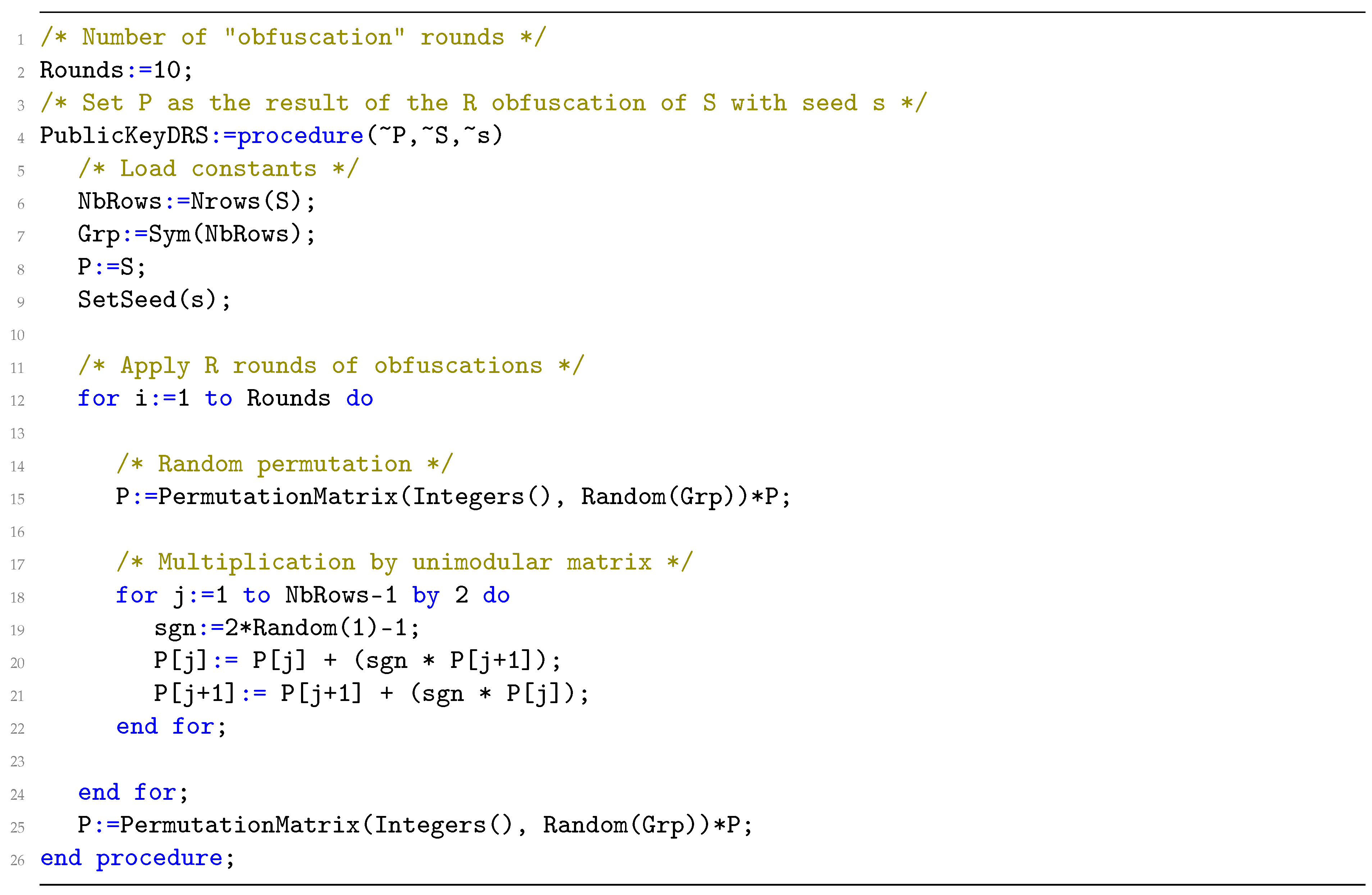
4.1.2. Public Key Generation

The lattice of the public key $P_k$ is the same lattice as the secret key $S_k$. However, we provide a different basis, which is more in tune with a classical GGH approach of “good” and “bad” basis. Roughly speaking, we need to provide an unimodular transformation matrix T such that $P_k=T{S}_k$. We have three objectives:

• Construct T in a fast manner, from a large combinatorial set.
• Bound the coefficients of $P_k$, making sure computations do not overflow.
• Make sure $T^{-1}$ is hard to reconstruct.

The third objective will rely on assumptions, as we cannot prove it at this point for any T (except specific unique forms like the HNF). The first two objectives, however, are reasonably achievable. First of all, we can easily to include permutation matrices to construct T: They respect the first two objectives. However, in the case of diagonal matrices, it is easy to see the third point is discarded with just permutations: A diagonal dominant structure is easy to “permute” back. The problem then will be to intermingle row vectors and control their growth without changing the lattice generated. We here choose the intermingling of 2 vectors to be equivalent to a multiplication of random pairs of vectors (a $2\times n$ matrix) by a square unimodular matrix of dimension 2 and maximum norm of 2.

The set $U_{\{+,-\}}$ of the unimodular matrices we use for the purpose of intermingling vectors is very particular:

$$U_{\{+,-\}}=\left\{U_{+}=\left[\begin{array}{cc}1& 1\\ 1& 2\end{array}\right],U_{-}=\left[\begin{array}{cc}1& -1\\ -1& 2\end{array}\right]\right\}$$

and let us define the set $U_{\{+,-\}}^{\prime }$ constructed from $U_{\{+,-\}}$:

$$U_{\{+,-\}}^{\prime }=\left\{\forall i\in [1,n/2],U_i\in U_{\{+,-\}}:\left[\begin{array}{ccccc}{U}_0& 0& \cdots & & 0\\ 0& U_1& \ddots & & \\ ⋮& 0& \ddots & \ddots & ⋮\\ & & \ddots & U_{n/2-1}& 0\\ 0& \cdots & & 0& U_{n/2}\end{array}\right]\right\}$$

Let $P\in S_n$ a permutation matrix and $U\in U_{\{+,-\}}^{\prime }$, and M a structured matrix we want to make hard to recover. We can conceive a “round” of scrambling to be the transformation $M\leftarrow UPM$. In our case one single round of scrambling is obviously not enough. Therefore, we need to scramble multiple times, each new round being applied with a new randomly selected tuple $(U,P)$. Let R be the number of such rounds. Our choice for T such that $P_k=T{S}_k$ is thus:

$$U=P_{R+1}{\prod }_{i=1}^R{U}_i{P}_i$$

i.e., a combination of $R+1$ permutations and R intermingling of vectors.

The number of rounds R is decided upon security consideration but also efficiency reasons as we wanted to fit every computation within 64-bits. Each round multiplies the maximum size of the coefficients (we will denote $\delta$) by a factor at most 3. Note that the case 3 is rare. The number R is dependent of other parameters we will explain later.

The public key is thus by successive additions/substractions of pair of vectors (see Algorithm 4). Note that the only difference with the original scheme [14] is that we do not store the ${log}_2$ of the maximum norm. We estimate this information to be easily computed at negligeable time. A MAGMA code can be found in the appendix (see code Figure A2).

Algorithm 4 Public key generation
Require:$S=D_{Id}-M$ the reduction matrix, a random seed x
Ensure:P such that $\mathcal{L}\left(P\right)=\mathcal{L}\left(S\right)$ and ${\parallel S\parallel }_{\infty }{<<\parallel P\parallel }_{\infty }\le 3^R{\parallel S\parallel }_{\infty }$
1: $P\leftarrow S$
2: $InitiateRdmSeed\left(x\right)$	▹ Sets the randomness via x
3: for $i=1$ ; $i<R$ ; $i=i+1$ do
4:  $P\leftarrow \mathbf{RdmPmtn}\left(P\right)$	▹ Shuffle the rows of P
5:  for $j=1$ ; $j\le n-1$ ; $j=j+2$ do
6:    $t\leftarrow \mathbf{RdmSgn}\left(\right)$
7:    $P\left[j\right]=P\left[j\right]+t\ast P[j+1]$	▹ “Random” linear combinations
8:    $P[j+1]=P[j+1]+t\ast P\left[j\right]$
9: $P\leftarrow \mathbf{RdmPmtn}\left(P\right)$
10: return P

The power of 2 $p_2$ we removed from the descrition has no security impact, and is used mostly for the verification process to make sure intermediate computation results stay within 64-bits. This type of public key is very different from the HNF [15] suggested to use; however, the computation time of a HNF is non-negligible. As we will see later this directly impact the signature.

4.2. Signature

Rather than checking if the successive approximation of Babai’s algorithm on a vector m of converges [15], DRS checks if the successive approximation on a vector m can reach a point where ${\parallel m\parallel }_1<nD$, and if $\exists i,|m_i|>D$, reduce m further without increasing ${\parallel m\parallel }_1$.

Given the fact that the secret key is a diagonally dominant matrix, Algorithm 5 is guaranteed to complete: forcing $tr\left(M\right)=0$ on the noise, we presented a proof that ignored the convergence of the reduction steps but showed the existence of a reachable valid solution for ${\parallel m\parallel }_{\infty }<D$. A MAGMA code of the signing algorithm can be found in the appendix (see the code Figure A3). In a certain sense, it uses the fact that the PSW vector reduction algorithm (Algorithm 2) does not need to converge to find a solution. The original proof can be seen in [14]; however, we are not going to mention it here since a better proof will be shown after modification.

Algorithm 5 Sign: Coefficient reduction first, validity vector then
Require:$v\in {\mathbb{Z}}^n$, $(x,S)$ the secret seed and diagonal dominant matrix
Ensure:w with $v\equiv w\left[\mathcal{L}\right(S\left)\right]$, ${\parallel w\parallel }_{\infty }<D$ and k with $kP=v-w$
1: $w\leftarrow$v, $i\leftarrow 0$, $k\leftarrow [0,\dots ,0]$
2: while ${\parallel w\parallel }_{\infty }<D$ do	▹ Apply the PSW vector reduction
3:  $q\leftarrow w_i/D$
4:  $k_i\leftarrow k_i+q$	▹ Ensure $kS=v-w$
5:  $w\leftarrow w-qS\left[i\right]$
6:  $i\leftarrow i+1$ mod n
7: $InitiateRdmSeed\left(x\right)$	▹ Set randomness identical to Setup
8: for $i=1$ ; $i\le R$ ; $i=i+1$ do	▹ Transform $kS=v-w$ into $kP=v-w$
9:  $k\leftarrow \mathbf{RdmPmtn}\left(k\right)$
10:  for $j=1$ ; $j\le n-1$ ; $j=j+2$ do
11:    $t\leftarrow \mathbf{RdmSgn}\left(\right)$
12:    $k[j+1]=k[j+1]-t\ast k\left[j\right]$
13:    $k\left[j\right]=k\left[j\right]-t\ast k[j+1]$
14: $k\leftarrow \mathbf{RdmPmtn}\left(k\right)$
15: return$k,v,w$

Another difference with the original PSW is the fact that it did not have a second vector k to output in their initial scheme and thus only had to deal with the reduction part [15]. The vector k is needed to ensure $v-w\in \mathcal{L}\left(P_k\right)$, which in the case of a HNF was not needed as the triangular form allowed an easy verification.

Note that if we wish to fit every computation within 64-bits, then we need to enforce ${log}_2\parallel k\parallel <63$. Thus we need to bound it with previous parameters, i.e.,

$$k^{\prime }(D-M)=v-w$$

$$\parallel k^{\prime }{\parallel \le \parallel v-w\parallel \parallel (D-M)}^{-1}\parallel$$

$$\parallel k^{\prime }\parallel \le \parallel v-w\parallel \parallel D^{-1}\frac{1}{1-\frac{M}{D}}\parallel$$

$$\parallel k^{\prime }\parallel \le \parallel v-w\parallel \parallel D^{-1}\parallel \parallel \frac{1}{1-\frac{M}{D}}\parallel$$

$$\parallel k^{\prime }\parallel \le \parallel v-w\parallel \parallel D^{-1}\parallel \parallel \parallel 1+\frac{M}{D}+{\left(\frac{M}{D}\right)}^2+\dots \parallel$$

$$\parallel k^{\prime }\parallel \le \parallel v-w\parallel \parallel D^{-1}\parallel (\parallel 1\parallel +\parallel \frac{M}{D}\parallel +\parallel \frac{M}{D}{\parallel }^2+\dots )$$

$$\parallel k^{\prime }\parallel \le \parallel v-w\parallel \parallel D^{-1}\parallel \parallel \frac{1}{1-\parallel \frac{M}{D}\parallel }\parallel$$

$$\parallel k^{\prime }\parallel \le \parallel v-w\parallel \parallel \frac{1}{D-\parallel M\parallel }\parallel$$

$$\parallel k^{\prime }\parallel \le \parallel v-w\parallel \frac{1}{\Delta }$$

$$\parallel k^{\prime }\parallel \le (\delta +1)\frac{1}{\Delta }=\frac{\delta +1}{\Delta }$$

therefore:

$$\begin{array}{cc}\hfill k& =k^{\prime }{U}^{-1}\hfill \\ \hfill \parallel k\parallel & \le \parallel k^{\prime }\parallel \parallel U^{-1}\parallel \hfill \\ \hfill \parallel k\parallel & \le \parallel \frac{\delta +1}{\Delta }\parallel \parallel U^{-1}\parallel \hfill \\ \hfill \parallel k\parallel & \le \frac{(\delta +1)3^R}{\Delta }\hfill \end{array}$$

thus giving us the means to fix $\Delta ,\delta ,R$ to fit every coefficients within 64-bits.

4.3. Verification

Given a hashed message vector v, the signature $(k,w)$, the verification is reduced to the equality test $k{P}_k=(v-w)$. However, as the computation $k{P}_k$ might overflow (the maximum size of k depends of $\delta ,\Delta ,R$, and $P_k$’s ones from $D,R$). In the following verification algorithm we recursively cut k into two parts $k=r+p_{2}q$ where $p_2$ is a power of 2 that is lower than $2^{63}/\parallel P_k\parallel$, which ensures $r{P}_k$ is not overflowing.

Given $P_k,2^k$, $t=v-w$ and $k=r+p_{2}q$ with $\parallel r\parallel <p_2$, we have $k{P}_k-t=c$ with $c=0$ if and only if $k{P}_k=v-w$. Therefore

$$q{p}_2{P}_k+r{P}_k-t=c\to q{P}_k=\frac{c+t-r{P}_k}{p_2}$$

and thus $p_2$ should divide $t-r{P}_k$ if $c=0$: If not, that means $c\ne 0$ and the verification returns FALSE. Otherwise, we set $k^{\prime }\leftarrow q$ and $t^{\prime }\leftarrow t-r{P}_k$ and repeat

$$(q{P}_k-\frac{t-r{P}_k}{p_2}=\frac{c}{p_2})\to (k^{\prime }{P}_k-t^{\prime }=c^{\prime })$$

where $c^{\prime }$ becomes exactly the integer $c/p_2$ regardless of its value (if it didn’t fail before). The verification stops when both $t^{\prime }=0$ and $k^{\prime }=0$. Note that both need to be 0 at the same time, if only one of them is 0 then the verification fails.

The verification, given $k,v,w,P_k$ is then as follow in Algorithm 6. Note that the core algorithm could be optimized but we just give here the overall idea. A MAGMA code is provided in the appendix (see code Figure A5) for testing purposes.

Algorithm 6 Verify
Require:$v,w,k\in {\mathbb{Z}}^n$, P the public key
Ensure: Checks $v\equiv w\left[\mathcal{L}\right(P\left)\right]$ and ${\parallel w\parallel }_{\infty }<D$
1: if ${\parallel w\parallel }_{\infty }>=D$ then	▹ Checks ${\parallel w\parallel }_{\infty }<D$
2:  return FALSE
3: $q\leftarrow k$
4: $t\leftarrow v-w$
5: $p_2\leftarrow {log}_2{\parallel P\parallel }_{\infty }$
6: while $q\ne 0\wedge t\ne 0$ do	▹ Verification per block of size $p_2$
7:  $r\leftarrow$$q-(p_2\times \lceil q/p_2\rfloor )$	▹ Get the smallest sized remainder
8:  $t\leftarrow t-(r\ast P)$
9:  if $t\ne 0mod{p}_2$ then	▹ Check block
10:    return FALSE
11:  $t\leftarrow t/p_2$	▹ Update values for next iteration
12:  $q\leftarrow (q-r)/p_2$
13:  if $(t=0)⊻(q=0)$ then
14:    return FALSE
15: return TRUE

If multiprecision integers were to be used (as using GNU Multiple Precision Arithmetic Library (GMP)), it would not take a while loop with multiple rounds to check. Whether this is more efficient or not remains to be tested.

Example 3.

Verification example for $p_2=10000$:

$$P=\left[\begin{array}{cccccc}-1840& 2471& -382& -820& 710& 3048\\ 1966& -1378& 1486& 1721& 1430& -4090\\ -1998& 4317& 994& 271& 3660& 2211\\ 2729& -3460& 746& 1375& -680& -4662\\ 2784& -6566& -1866& -801& -6100& -2700\\ 3679& -3323& 2144& 2716& 1380& -7160\end{array}\right]$$

$$k=\left[\begin{array}{cccccc}-54029& -77227& 6908& -38654& -4594& 50148\end{array}\right]$$

$$v=\left[\begin{array}{cccccc}924& 232& 131& 692& 439& 694\end{array}\right]$$

$$w=\left[\begin{array}{cccccc}0& 9& -9& -1& -1& 0\end{array}\right]$$

Goal: Verify$kP=v-w=\left[\begin{array}{cccccc}924& 223& 140& 693& 440& 694\end{array}\right]$with low size computations. Set $q=k$ and $t=v-w$.

$$\mathit{First} \mathit{pass}:$$

$$r\leftarrow qmod{p}_2=\left[\begin{array}{cccccc}-4029& 2773& -3092& 1346& -4594& 148\end{array}\right]$$

$$t\leftarrow t-r\times P=\left[\begin{array}{cccccc}-10470000& 2110000& -12480000& -13170000& -17100000& 25390000\end{array}\right]$$

$$t \mathit{is} \mathit{clearly} \mathit{divisible} \mathit{by} p_2, \mathit{update} q, t$$

$$q\leftarrow (q-r)/p_2=\left[\begin{array}{cccccc}-5& -8& 1& -4& 0& 5\end{array}\right]$$

$$t\leftarrow t/p_2=\left[\begin{array}{cccccc}-1047& 211& -1248& -1317& -1710& 2539\end{array}\right]$$

$$\mathit{Both} \mathit{are} \mathit{non}-\mathit{zero} \mathit{Repeat}.$$

$$\mathit{Second} \mathit{pass}:$$

$$r\leftarrow kmod{p}_2=\left[\begin{array}{cccccc}-5& -8& 1& -4& 0& 5\end{array}\right]$$

$$t\leftarrow t-r\times P=\left[\begin{array}{cccccc}0& 0& 0& 0& 0& 0\end{array}\right]$$

$$t \mathit{is} \mathit{clearly} \mathit{divisible} \mathit{by} p_2, \mathit{update} q, t \mathit{and} \mathit{continue}$$

$$q\leftarrow (q-r)/p_2=\left[\begin{array}{cccccc}0& 0& 0& 0& 0& 0\end{array}\right]$$

$$t\leftarrow t/p_2=\left[\begin{array}{cccccc}0& 0& 0& 0& 0& 0\end{array}\right]$$

$$\mathit{Both} \mathit{are} \mathit{zero}.\mathit{End} \mathit{with} \mathit{true}.$$

5. On the Security of the Public Key

Note that the public key of DRS relies on successive multiplication of heavily structured $2\times 2$ matrices. There is no concrete security reduction or previous examples in the literature to assert the security of this type of public key. However, the main objective of the public key setup of DRS was to “evenly distribute” the coefficients around all positions while ensuring the setup could never overflow (on 64-bits processors). If this specific method ever finds a weakness, we could either use a HNF which can be computed in polynomial time [30], or use other types of unimodular matrices. GGH for example used triangular matrices to generate their keys. Other methods of sampling are welcomed; however, to the best of our knowledge the HNF still provides optimal safety as it is unique per lattice and an attack on the structure of the HNF is therefore, an attack on all possible basis [8].

The problem with a HNF is its computation time and the objects we need to manipulate: Multiprecision library are often needed and computation time for cryptographically secure sizes goes well over a dozen of seconds even on high-end computers, which is a severe flaw for a lot of applications. While speeding up the computations for this particular type of keys might be possible, it was; however, not the point of our work so far. We here focus on patching the structure of the secret key, as this is the only angle where flaws were discovered in the literature.

5.1. Li, Liu, Nitaj and Pan’s Attack on a Randomized Version of the Initial PKC’08

In ACISP 2018, Li, Liu, Nitaj and Pan [17] presented an attack that makes use of short signatures to recover the secret key. Their observation is that two different signatures from the same message is also a short vector of the lattice. Then, gathering sufficient number of short vectors enable easier recovery of the secret key using lattice reduction algorithms with the vectors generated. Their suggestion to fix this issue is to either store previous signed messages to avoid having different signatures, or padding a random noise in the hash function. We should note that the initial DRS scheme is not randomized as the algorithm is deterministic and produce a unique signature per vector.

We do note that the authors of DRS suggested in their report [14] to use a random permutation to decide the order of the coefficent reduction, and thus Li, Liu, Nitaj and Pan’s attack might apply to their suggestion. However, the order of the coefficient reduction could also be decided deterministically by the hashed message itself, and therefore, Li, Liu, Nitaj and Pan’s attack is not fully applicable, as this method would produce an unique signature per message. They can still generate a set of relatively short vectors $(r_1,\dots ,r_2)\in {\mathcal{L}}^n$ of the lattice $\mathcal{L}$; however, it is unclear whether the specialized version of their attack using vectors s,$(v_1,\dots ,v_n)$ where $s-v_i\in \mathcal{L}$ is still applicable. It seems to be easier to recover the key when using multiple signatures from the same message as a lattice basis when using lattice reduction algorithms rather than using random small vectors of the lattice: This could imply that diagonal dominant basis have inner weaknesses beyond the simple instantiation of DRS. From our understanding, the secret key matrices they generated for their tests used a noise matrix $M\in {\{-1,0,1\}}^{n\times n}$, which could have had an impact in their experimentations. It is still unknown if other noise types such as the ones in DRS or the type of noise we are about to propose are affected: To the best of our knowledge, DRS was not quoted in their work.

We stress that we do not claim the new setup to be perfectly secure against Li, Liu, Nitaj and Pan’s attack, we merely claim more experimentations would need to be done as of now. Furthermore, the countermeasures proposed by Li, Liu, Nitaj and Pan also apply to those new keys, and should be applied if one wishes for a more concrete security. The next attack, however, does not have clear known countermeasures as of now and is the main focus of this paper.

5.2. Yu and Ducas’s Attack on the DRS Instantiation of the Initial Scheme of PKC’08

We explained in the previous section about the security of DRS against Li, Liu, Nitaj and Pan’s attack. On the other hand, it is unclear if such a modification would add an extra weakness against Yu and Ducas’s heuristic attack. Their attack work in two steps. The first one is based on recovering certain coefficients of a secret key vector using machine learning and statistical analysis. The second is classical lattice-reduction attack to recover the rest of the secret key.

For the first step, Yu and Ducas noticed that the coefficients B of the secret key and the 1 could be distinguished via machine learning techniques [16], noticing for one part that the non-diagonal coefficients follow an “absolute-circulant” structure, and the fact that only two types of non-zero values exist. Based on this information, a surprisingly small amount of selected “features” to specialize a “least-square fit” method allowed them to recover both positions and signs of all if not most coefficients B of a secret vector. We note they did not conduct a exhaustive search on all possible methods according to their paper thus stressing that their method might not be the best. We did not conduct much research on the related machine learning techniques; therefore, we cannot comment much on this part as of now.

A few points were presented to explain why their technique works. One point is the difference between the noise coefficients: It was either close to non-existant or very large, causing wave-shaped reductions that could be detected given enough samples. The other point is that this wave-shaped reduction is absolute-circulant, which makes the structure more obvious as this wave-shaped perturbation translates in incremental order. Figure 2 is a visual representation of the cascading phenomenon, taken directly from [16] (S is a secret key vector and w a vector to reduce).

On the second step, the recovered coefficients and their positions and signs allowed them to apply the Kannan embedding attack on a lattice with the exact same volume as the original public key but of a much lower dimension than the original authors of DRS based their security on, by scrapping the known B noise coefficients. Strictly speaking, using the same notation as in the previous description of DRS and assuming the diagonal coefficient is equal to the dimension, the initial search of a shortest vector of length $\sqrt{B^2{N}_b+N_1+1}$ in a lattice of dimension n of determinant $n^n$ becomes a search of a shortest vector of length $\sqrt{N_1+1}$ in a lattice of dimension $n-N_b$ of determinant $n^n$. A visual representation on the effect of this attack can be seen in the next section or in Example 2 where all big red coefficients are replaced by 0 in one basis vector. The efficiency of lattice reduction techniques then affects the evaluation of the security strength of the original DRS scheme.

Yu and Ducas conducted experiments and validated their claims using only a few dozens of thousands of signatures per key, reducing the security of the initial submission of DRS from 128-bits to maybe at most 80-bits, using BKZ-138. The original concept (not the instantiation) from [15], however, still seems to be safe for now: While it has no security proof, to the best of our knowledge, no severe weaknesses have been found so far. Furthermore, Yu and Ducas advised of some potential countermeasures to fix DRS, i.e., breaking the structure of the particular instance that was submitted: The deterministic approach of the number of B, 1, being limited to those two values (5 if we consider zeroes and signs), and the “absolute-circulant” structure. They also pointed that a lack of security proof could be problematic and gave some opinions about how one can potentially find provable security for the DRS scheme.

We invite readers to read their work: It is possible that new techniques relying on machine learning could apply to all lattice-based cryptosystems beyond DRS by tweaking their process for each specific structure.

In the following section, we provide a countermeasure which follows some of the recommendations given by Yu and Ducas as breaking the secret key noise structure and giving some statistical heuristic, while still preserving the original idea given in PKC 2008 [15].

6. New Setup

We do not change any algorithm here aside the setup of the secret key: The public key generation method is left unchanged, along with the signature and verification. Compared to the old scheme, this new version is now determined by less parameters, which leave 6 of them using the previous DRS: The dimension n, a random generator seed s, a signature bound D, a max norm for hashed messages $\delta$, a sparsity parameter $\Delta$ that we always set to one, and R a security parameter determining the number of multiplication rounds to generate the public key.

We choose random noise among all the possible noises vectors which would still respect the diagonal dominant property of the secret key. This choice is following Yu and Ducas’s suggestions on breaking the set of secret coefficients, the “absolute-circulant” structure of the secret key, and allowing us to provide statistical evidence. Roughly speaking, we aimed to transform the following structure of

$$\left[\begin{array}{cccccc}\mathbf{15}& 0& 0& 0& 0& 0\\ 0& \mathbf{15}& 0& 0& 0& 0\\ 0& 0& \mathbf{15}& 0& 0& 0\\ 0& 0& 0& \mathbf{15}& 0& 0\\ 0& 0& 0& 0& \mathbf{15}& 0\\ 0& 0& 0& 0& 0& \mathbf{15}\end{array}\right]+\cancel{\bcancel{\left[\begin{array}{cccccc}0& 5& 1& 0& -1& 1\\ -1& 0& -5& 1& 0& -1\\ -1& 1& 0& 5& 1& 0\\ 0& 1& 1& 0& 5& -1\\ 1& 0& -1& 1& 0& -5\\ 5& -1& 0& 1& -1& 0\end{array}\right]}}$$

to something “less-structured”, more “random” but still diagonal dominant like

$$\left[\begin{array}{cccccc}\mathbf{15}& 0& 0& 0& 0& 0\\ 0& \mathbf{15}& 0& 0& 0& 0\\ 0& 0& \mathbf{15}& 0& 0& 0\\ 0& 0& 0& \mathbf{15}& 0& 0\\ 0& 0& 0& 0& \mathbf{15}& 0\\ 0& 0& 0& 0& 0& \mathbf{15}\end{array}\right]+\left[\overline{)\begin{array}{cccccc}4& -2& 0& 3& -1& 4\\ -2& 3& -1& 0& -8& 0\\ 6& 1& 2& -1& 1& 3\\ 0& 0& -4& 3& 2& 3\\ -3& 2& -1& -3& -1& 3\\ 1& -1& 2& -4& -4& 2\end{array}}\begin{array}{c}=14\\ =14\\ =14\\ =12\\ =13\\ =14\end{array}\right]$$

While we want to have random noise, we must ensure we can still sign every message and thus guarantee the diagonal dominant structure of our secret key. Hence, the set of noise vectors we need to keep are all the vectors $v\in {\mathbb{Z}}^n$ that have a taxicab norm of ${\parallel v\parallel }_1\le D-1$. Let us call that set $V_n$.

Sampling from $V_n$, however, is no trivial task. However, preceding work in the academic literature allows us to:

• Count all points of ${\mathbb{Z}}^n$ inside a n-ball for the $l_1$-norm, i.e., $|V_n|$. [31]
• Know how many of them have a fixed amount of zeroes. [31]
• Sample uniformly from the n-simplex, fixing a certain amount of zeroes. [32]

Therefore, the plan is the following:

• Creates a cumulative frequency distribution table from [31].
• Use the table to sample uniformly a number of zeroes.
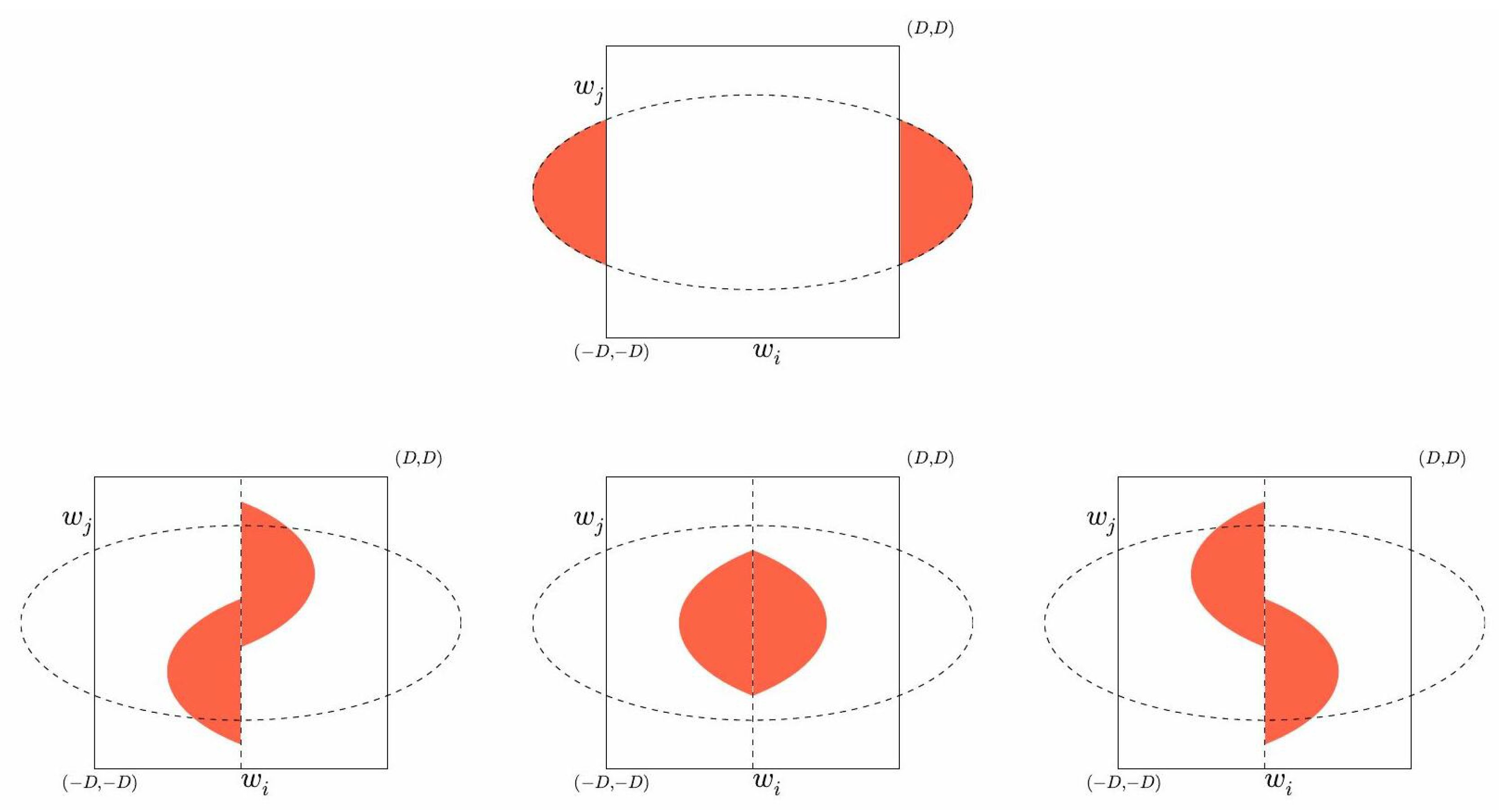
• Sampling uniformly within the n-ball of with a fixed number of zeroes.

This new setup will also change the bounds used for the public key, as the original DRS authors linked several parameters together to ensure computations stay within 64 bits. However, our paper has a more theoretical approach and we do not focus on the technical implementations.

6.1. Picking the Random Vectors

We are aiming to build the new noise matrix M, which is a $n\times n$ matrix such that $M\in V_n^n$. In that regard, we construct a table we will call T with D entries such that

$$T\left[i\right]=\#\mathrm{vectors} v\in V_n\mathrm{with}i\mathrm{zeroes}.$$

This table is relatively easy to build and does not take much time, one can for example use the formulas derivated from [31,33].

From this table, we construct another table $T_S$ such that $T_S\left[k\right]={\sum }_{i=0}^{k}T\left[i\right]$.

The generation algorithm of the table $T_S$, which we will use as a precomputation for our new setup algorithm can be seen in Algorithm 7.

Algorithm 7 Secret key table precomputation
Require: all initial parameters
Ensure:$T_S$ the table sum
1: $m\leftarrow \mathbf{min}(n,D)$
2: $T\leftarrow {\left\{1\right\}}^{m+1}$
3: $T_S\leftarrow {\left\{1\right\}}^{m+1}$
4: for $j=2$ ; $j\le D$ ; $j=j+1$ do	▹ Loop over the norm
5:  for $i=2$ ; $i\le m+1$ ; $i=i+1$ do	▹ Loop over possible non-zeroes
6:    $x\leftarrow 2^{i-1}\left(\genfrac{}{}{0pt}{}{n}{i-1}\right)\left(\genfrac{}{}{0pt}{}{j-1}{i-2}\right)$
7:    $T[m+1-i]\leftarrow T[m+1-i]+x$
8: for $i=1$ ; $i\le m$ ; $i=i+1$ do	▹ Construct array $T_S$ from T
9:  $T[i+1]\leftarrow T[i+1]+T\left[i\right]$
10: $T_S\leftarrow T$
11: return $T_S$

Let us denote the function $Z\left(x\right)\to y$ such that $T_S[y-1]<x\le T_S\left[y\right]$. Since $T_S$ is trivially sorted in increasing order $Z\left(x\right)$ is nothing more than a dichotomy search inside an ordered table. If we pick randomly x from $[0;T_S[D-1]]$ from a generator with uniform distribution $g\left(\right)\to x$ then we got $Zero\left(\right)\to Z\left(g\right(x\left)\right)$ a function that selects uniformly an amount of zeroes amount all vectors of the set $V_n$, i.e.,

$$Zero\left(\right)\to \#\mathrm{zeroes} \mathrm{in}\mathrm{a}\mathrm{random}v\in V_n$$

Now that we can generate uniformly the number of zeroes we have to determine the coefficients of the non-zero values randomly, while making sure the final noise vector is still part of $V_n$. A method to give such a vector with chosen taxicab norm is given in [32] as a correction of the Kraemer algorithm. As we do not want to choose the taxicab norm M directly but rather wants to have any random norm available, we add a slight modification: The method in [32] takes k non-zero elements $x_1,\dots ,x_k$ such that $x_i\le x_{i+1}$ and forces the last coefficient to be equal to the taxicab norm chosen, i.e., $x_k=M$. By removing the restriction and using $x_k\le D$, giving the amount of non-zero values, we modify the method to be able to take over any vector values in $V_n$ with the help of a function we will call

$$\mathbf{KraemerBis}\left(z\right)\to \mathrm{random}v\in V_n$$

such that v has z zeroes which is described in Algorithm 8.

Algorithm 8 KraemerBis
Require: all initial parameters and a number of zeroes z
Ensure: a vector v with z zeroes and a random norm inferior or equal to D
1: $v\in {\mathbb{N}}^n$
2: $0\le x_0<x_1<\dots <x_{n-z}\le D$	▹ Pick randomly $n-z+1$ elements
3: for $i=1$ ; $i\le n-z$ ; $i=i+1$ do
4:  $v\left[i\right]\leftarrow x_i-x_{i-1}$
5: for $i=n-z+1$; $i\le n$; $i=i+1$ do
6:  $v\left[i\right]\leftarrow 0$
return v

With both those new parts, the new setup algorithm we construct is presented in Algorithm 9 using Kraemer bis. We note that in our algorithm, the diagonal coefficient in the secret key is not guaranteed to be equal to the bound used for the maximum norm of the signatures. Nevertheless, we will show that the termination is still ensured in Section 6.2. This heavy setup naturally affects the speed of the DRS setup, as we noticed in our experiments as shown in Section 6.5.

Algorithm 9 New secret key generation
Ensure: all initial parameters and another extra random seed x
Require:$x,S$ the secret key
1: $S\leftarrow D_{Id}$
2: $t\in {\mathbb{Z}}^n$
3: $InitiateRdmSeed\left(x\right)$	▹ Set randomness
4: for $i=1$ ; $i\le n$ ; $i=i+1$ do
5:  $Z\leftarrow Zero\left(\right)$	▹ Get the number of zeroes
6:  $t\leftarrow \mathbf{KraemerBis}\left(Z\right)$
7:  for $j=1$; $j\le n-Z$; $j=j+1$ do	▹ Randomly switch signs
8:    $t\left[j\right]\leftarrow t\left[j\right]\times \mathbf{RdmSgn}\left(\right)$
9:  $t\leftarrow \mathbf{RdmPmtn}\left(t\right)$	▹ Permutes everything
10:  $S\left[i\right]\leftarrow S\left[i\right]+t$
11: return $x,S$

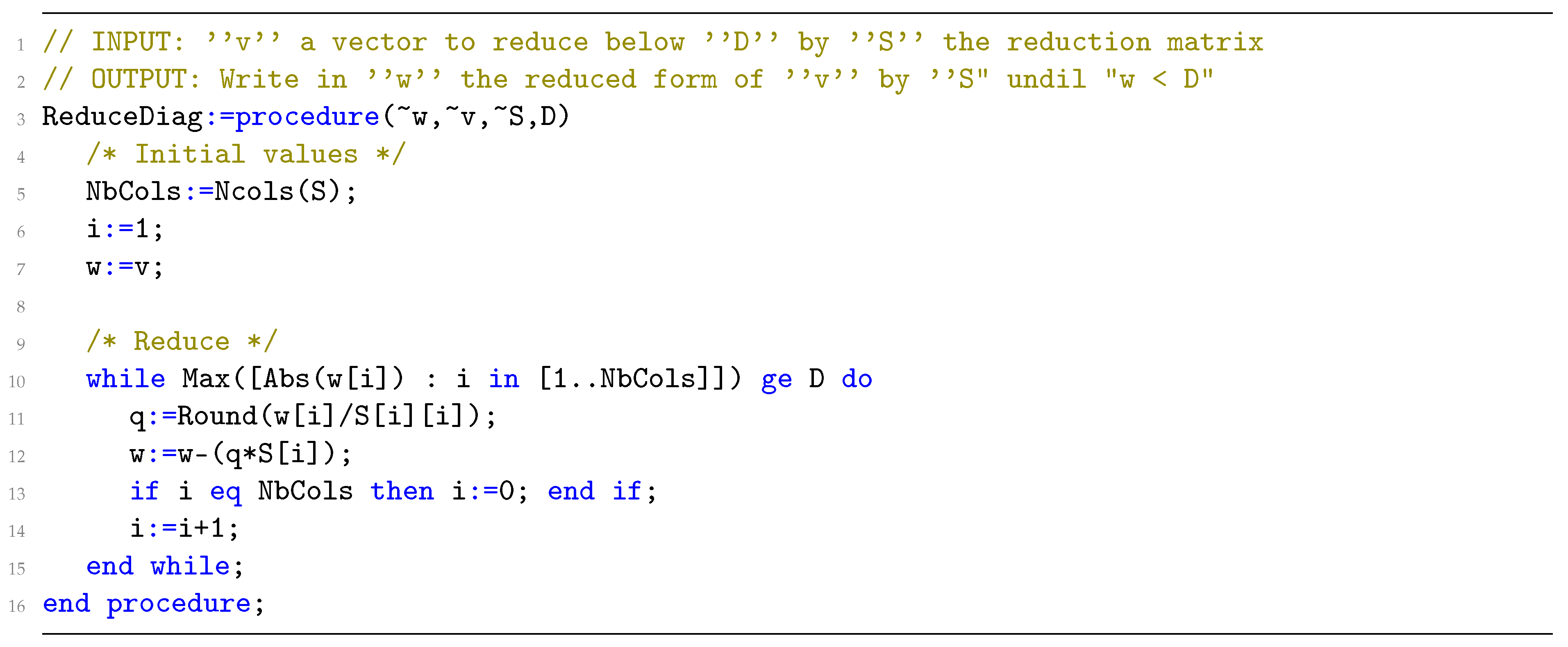
6.2. A Slightly More General Termination Proof

The proof stated in the DRS report on the NIST website [14] was considering that the diagonal coefficient of $S=D_{Id}+M$ stayed equal to the signature bound (i.e., $tr\left(M\right)=0$), which is not this case. We show here that the reduction is still guaranteed nevertheless. Suppose that some coefficients of the noise matrix M are non-zero on the diagonal. Re-using for the most part notations of the original report, where:

• m is the message we want to reduce, which we update step by step
• M is the noise matrix (so $M_i$ is the i-th noise row vector).
• D is the signature bound for which the condition ${\parallel m\parallel }_{\infty }<D$ has to be verified. We note $d_i$ the i-th diagonal coefficient of the secret key S.

Obviously, the matrix will still be diagonal dominant in any case. Let us denote $d_i$ the diagonal coefficient $S_{i,i}$ of $S=D_{Id}-M$.

If $D>d_i$ we can use the previous reasoning and reduce $\parallel m_i{\parallel }_1$ to $\parallel m_i{\parallel }_1<d_i<D$, but keep in mind we stop the reduction at $\parallel m_i{\parallel }_1<D$ to ensure we do not leak information about the noise distribution.

Now $d_i>D$ for some i: Reducing to $|m_i|<d_i$ is guaranteed but not sufficient anymore as we can reach $d<|m_i|<d_i\le D+\Delta <2d$. Let us remind that $\Delta =D-{\sum }_{j=1}^n\left|M_{i,j}\right|$, where $\Delta$ is strictly positive as an initial condition of the DRS signature scheme (both on the original submission and this paper), $d_i=D+c$ where $c=|M_{i,i}|$.

Without loss of generality as we can flip signs, let us set $m_i=D+k<d_i=D+c$ with $k\ge 0$ the coefficient to reduce. Substracting by $S_i$ transforms

$$m_i\leftarrow (D+k)-d_i=(D+k)-(D+c)=k-c<0$$

with $D>c>k\ge 0$. Therefore, the reduction of ${\parallel m\parallel }_1$ without the noise is

$${\parallel m\parallel }_1\leftarrow {\parallel m\parallel }_1-(D+k)+(c-k)={\parallel m\parallel }_1-(D-c)-2k.$$

but the noise contribution on other coefficients is at worst $(D-\Delta )-c$ thus

$${\parallel m\parallel }_1\leftarrow {\parallel m\parallel }_1-(D-c)-2k+(D-c-\Delta ).{\parallel m\parallel }_1\leftarrow {\parallel m\parallel }_1-2k-\Delta ={\parallel m\parallel }_1-(2k+\Delta ).$$

where $2k+\Delta >0$. Therefore, the reduction is also ensured in the case $d_i>D$.

6.3. On Exploiting the Reduction Capacity for Further Security

Remark that the proof hints at the fact we can actually lower the norm ${\parallel m\parallel }_1$ of some vector m to some value lower than D. It is easy to see that when $M=0$ and $S=D_{Id}$, every coefficient of m can be reduced to ${\parallel m\parallel }_1<D/2$ in exactly n iterations of the PSW vector reduction algorithm. Clearly, there should be some gap between the bound D and the amount of noise in M that can be filled. If we do fill that gap, we can extend the number of available keys to use by extending the set of applicable noise and hopefully making cryptanalysis harder. While it is hard to find examples in a “printable” size where the PSW Conjecture (Conjecture 1 in Section 3.2) applies while the DRS reduction proof does not, it becomes easier as the dimension grows. Using the code in Figure A6 gives us an example on the gap between the PSW conjecture and the DRS proof. The output is shown in Figure 3

We can see in Figure 3 that every noise vector comfortably goes over the DRS bound (here $D=51$) while $\rho \left(M{D}^{-1}\right)\approx 0.49<0.5$. Note that the opposite is also true: By changing the noise to enforce the respect of the DRS bound (commenting line 14 and uncommenting line 16 of code in Figure A6), we can obtain the inverted result as seen in Figure 4.

One part of an explanation to this phenomenon is that the sign does not affect the DRS bound while it does heavily affect the PSW bound. If weakness appears on this new DRS instantiation due to the noise being too low, intuitively we think increasing the bound of the n-dimensional ball from which we uniformly sample the noise should still lead to most keys being usable w.r.t the PSW-conjecture. However, we discuss in the following part methods to efficiently generate keys for PSW that are proven to respect the PSW conjecture. While they do seem to be relatively simple, establishing instances of a general PSW scheme beyond a noise $M\in {\{-1,0,1\}}^{n,n}$ seems to have been lacking in the literature. We hope this can help close the gap between the conclusions of DRS and PSW.

6.4. Ensuring the Termination of PSW

In this subsection we present simple ways for the PSW approach to be more practical. A first example can be found as early as in 1965 [34]. Let us rephrase the (among others) theorem given by Derzko and Pfeffer:

Theorem 3

(The 4th Derzko-Pfeffer theorem). Let $M,S\in {\mathbb{C}}^{n,n}$ where S is invertible. Then the following is always true:

$$\rho \left(M\right)\le {(1-1/n)}^{1/2}\{{\left(ϵ\left(SM{S}^{-1}\right)\right)}^2-|tr\left(M\right){|}^2/n\}+|tr\left(M\right)|/n$$

where $ϵ\left(A\right)=\sqrt{{\sum }_{i,j=1}^n{\left|M_{i,j}\right|}^2}$ is the Froebenius norm.

Now, using this theorem, let us attempt at constructing a noise matrix M. Setting $tr\left(M\right)=0$ on the noise, and fixing S as the canonical basis we obtain:

$$\rho \left(M\right)\le {(1-1/n)}^{1/2}{\sum }_{i,j=1}^n{\left|M_{i,j}\right|}^2$$

Now, we can rely on PSW conjecture forcing $\rho \left(M{D}_{Id}^{-1}\right)<1/2$ using a diagonal matrix $D_{Id}$:

$$2{(1-1/n)}^{1/2}{\sum }_{i,j=1}^n{\left|M_{i,j}\right|}^2\le D$$

i.e., given a fixed dimension n and a fixed value D, we can properly bound the values of the noise matrix M such that the PSW Conjecture is respected. This can be done by carefully distributing the coefficients outside the diagonal.

However, the first thing to notice is that the bound is worse than the one given in DRS in most cases: The DRS bound is per vector, and this one is per matrix. Quick comparisons between the total sum of matrix coefficients will show the DRS bound is almost always superior.

Another theorem we could use on spectral radius is Gelfand’s formula, which was also used in [15]:

Theorem 4

(Gelfand’s spectral radius formula). $\rho \left(M\right)={lim}_{k\to \infty }{\parallel M^k\parallel }^{1/k}$.

An extreme case would then to fix the limit to 0. This then warrants the uses of nilpotent matrices, i.e., matrices $M\in {\mathbb{Z}}^{n\times n}$ such that $\exists k>0,M^k=0$. We then need to have some form of generation for nilpotent matrices. One easy group of nilpotent matrices is the following:

For $M=\left[\begin{array}{ccc}{M}_1& \dots & M_1\\ M_2& \dots & M_2\\ ⋮& \dots & ⋮\\ M_{n-1}& \dots & M_{n-1}\\ -{\sum }_{i=1}^{n-1}{M}_i& \dots & -{\sum }_{i=1}^{n-1}{M}_i\end{array}\right]$, $M^2=0$.

As the values $M_i$ can be as large as wanted in this particular family, the DRS bound can be rapidly overblown, especially by the last row. We could also use other families of nilpotent matrices and combine them: The sum of nilpotent matrices being nilpotent, the space of possible noise could be large enough to ensure the security of cryptographic applications. However, it is unclear if using such matrices will allow efficient reductions: Large coefficients might hinder the convergence, and reaching a valid signature (if possible) might take unacceptable times for real-life cryptography. Furthermore, let us stress that the PSW-vector reduction is an approximation of Babai’s rounding off algorithm: Thus, if the initial basis is “bad”, then so could be the set of possible reduction results, i.e., having a noise with a zero-valued spectral radius is not enough. Therefore, a basis that is not diagonal dominant and have poor geometrical properties might not be suitable either.

Other approaches would be to remember that the spectral radius is the biggest eigenvalue (see Definition 17). Then we can attempt to use simple properties of the eigenvalues and control them to fix the exact value of the spectral value rather than bounding them. Let us look at the following: If M is a noise matrix, then $\rho \left(M\right)$ is the biggest value (in norm) that cancel the polynomial in $P\left(X\right)=\det (M-X_{Id})$. The literature on eigenvalues and their computations is extremely large [35]: Bartel–Stewart [36], Hessenberg-Schur [37], Householder [38], etc. It might be possible to reverse those methods and their subsequent works to construct a class of noise matrices respecting the PSW-conjecture. We also leave those studies for further work, as it likely requires much more studies. Overall, merging those approaches and the DRS approach into a uniform set of usable keys seems to be a widely open research question, let alone the computational practicability of those lattice classes (or subclasses).

For now, however, we provide practical efficiency tests on our new patch in the next subsection.

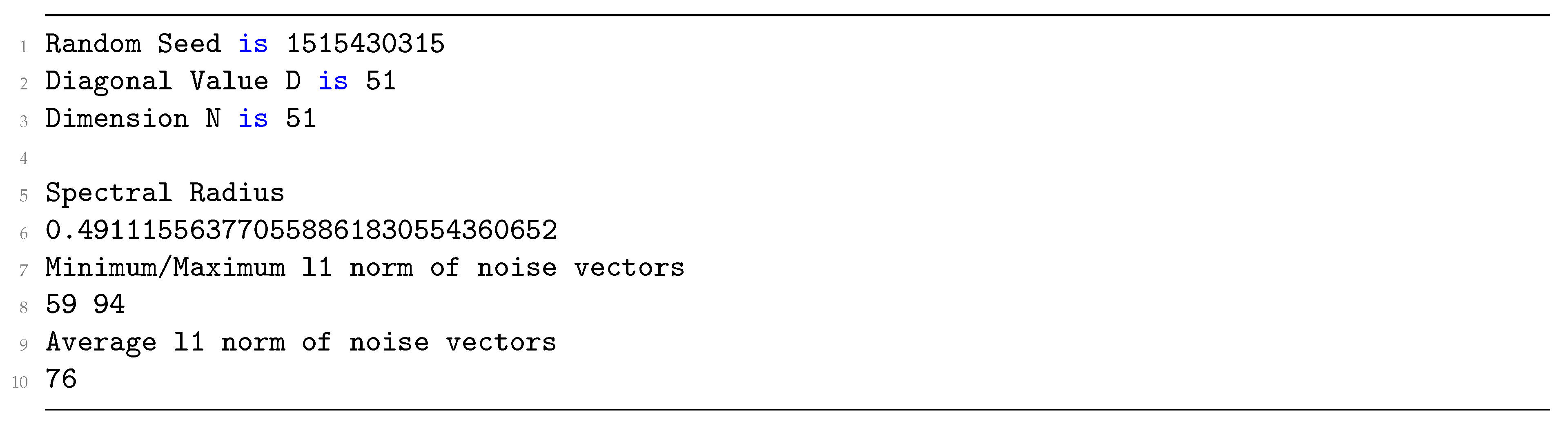
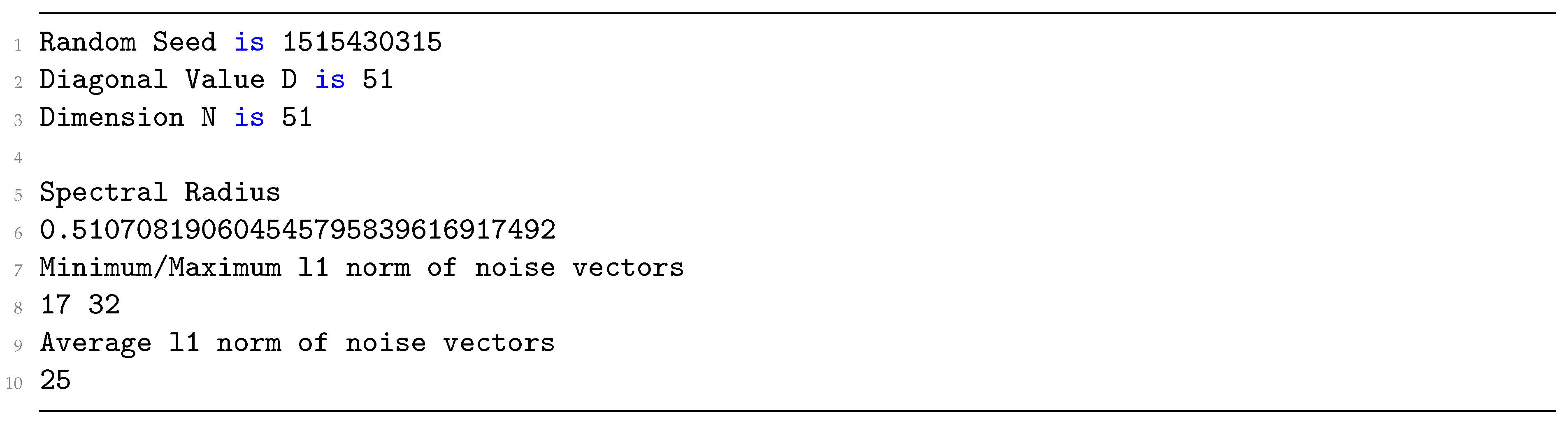
6.5. Setup Performance

Compared to the initial NIST submission where the code was seemingly made for clarity and not so much for performance, we wrote a modified version of DRS using NIST specifications and managed to have much higher performance. However, most of the performance upgrade from the initial code have nothing much to do with the algorithms of the DRS scheme: We did notice that most of the time taken by the DRS initial code was used for the conversion from the character arrays to integer matrices and vice-versa, which they had to do to respect the NIST specifications: The algebraic computations themselves were actually reasonably fast, considering the size of the objects manipulated.

This is the reason why we decided to isolate the secret matrix generation code from the rest of the initial original DRS code, in order to have a fair comparison between our own secret key generation algorithm to theirs. In that regard we choose to compare similar matrix sizes instead of similar security, as initial security estimates for the DRS submission were severely undermined by Yu and Ducas’s recent discoveries and thus would lead to comparing efficiency on matrices with massively different sizes. Therefore, we are making tests on the initial parameters of the DRS scheme. Looking purely at the secret key generation, we are indeed much slower, as shown in

Table 1. Secret key generation time in milliseconds (average for ${10}^4$ keys).

Dimension	912	1160	1518
OldDRS	2.871	4.415	7.957
NewDRS	31.745	63.189	99.392

.

Note that we use the options $-march=native$ and $-Ofast$ which led us to use $AVX512$ instructions and other $gcc$ optimization tweaks. The new setup is barely parallelizable as there is almost no code that can be vectorized which also explains the huge difference. While we wish to make a comparative performance to all other similar approaches, it seems the initial approach of PSW did not trigger further research and it remains an open topic, leaving DRS the only known fork of PSW to the best of our knowledge. Furthermore, timings were not provided in the original paper [15]: A figure illustrating the evolution of the number of reduction loops was deemed sufficient to demonstrate its efficiency back in 2008.

Moreover, note that in theory, sampling randomly using our method should not be a problem while growing the size of our keys if we only consider the time complexity. The problem, however, concerns the amount of data to store (and the related memory accesses). The size of $V_n$ grow more than exponentially and thus storing all related exact sizes could pose a problem for larger dimensions. A solution to drastically reduce the memory requirements would be to crop the extremely unlikely cases and round the remaining results, but so far this does not seem to be necessary for our largest parameters.

7. Security Estimates

The goal of this section is to evaluate the security of the scheme. First computationally by measuring the effectiveness of heuristic key-recovery attacks, and then by discussing the potential structural weakness of choosing diagonally dominant matrices as our key structure.

7.1. $BDD$-Based Attack

Currently, the most efficient way to perform this attack will be, first, to transform a BDD problem into a ${uSVP}_{\gamma }$ (Kannan’s Embedding Technique [39], assuming $v=(0,\dots ,0,d,0,\dots ,0)$, and use lattice reduction techniques on the lattice spanned by $\left[v\right|1]$ and the rows of $\left[B\right|0]$. By using this method, we obtain a $uSVP$ with a gap

$$\left(\begin{array}{cc}v& 1\\ B& 0\end{array}\right)$$

and second to solve this new ${uSVP}_{\gamma }$ using lattice reduction algorithm. By using this method, we obtain a ${uSVP}_{\gamma }$ with a gap

$$\gamma \approx \frac{\mathsf{\Gamma }{\left(\frac{n+3}{2}\right)}^{\frac{1}{n+1}}{Det\left(\mathcal{L}\right)}^{\frac{1}{n+1}}}{\sqrt{\pi }{\parallel M_1\parallel }_2}\approx \frac{\mathsf{\Gamma }{\left(\frac{n+3}{2}\right)}^{\frac{1}{n+1}}{d^n}^{\frac{1}{n+1}}}{\sqrt{\pi }{\parallel M_1\parallel }_2}.$$

(1)

Lattice reduction methods are well studied and their strength are evaluated using the Hermite factor. Let $\mathcal{L}$ a $d-$dimensional lattice, the Hermite factor of a basis B of $\mathcal{L}$ is given by ${\parallel B\left[1\right]\parallel }_2/det{\left(\mathcal{L}\right)}^{\frac{1}{n}}.$ Consequently, lattice reduction algorithms strengths are given by the Hermite factor of their expected output basis. In [21], it was estimated that lattice reduction methods solve ${uSVP}_{\gamma }$ with $\gamma$ a fraction of the Hermite factor. We will use a conservative bound of $\frac{1}{4}$ for the ratio of the ${uSVP}_{\gamma }$ gap to the Hermite factor. As we do not have a fixed Euclidean norm for our secret vectors we have to rely on the approximates given to us by our new random method in sampling noise vectors $M_i$. In our case, we know that for any vector $v\in {\mathbb{Z}}^n$ we have ${\parallel v\parallel }_2\ge \frac{{\parallel v\parallel }_1}{\sqrt{n}}$, and our experiments (as seen below) allow us to use a higher bound

$${\parallel v\parallel }_2⪆\sqrt{2}\frac{{\parallel v\parallel }_1}{\sqrt{n}}.$$

7.2. Expected Heuristic Security Strength

Different papers are giving some relations between the Hermite factor and the security parameter $\lambda$ [40,41] often using BKZ simulation [42]. Aiming to be conservative, we are to assume a security of $2^{128},2^{192},2^{256}$ for a Hermite factor of ${1.006}^d,{1.005}^d,{1.004}^d$, respectively. We set $D=n$, pick hashed messages $h\left(m\right)$ such that ${log}_2{(\parallel h\left(m\right)\parallel }_{\infty })=28$, $R=24$ and $\Delta =1$.

Table 2. Parameter sets.

Dimension	$\mathbf{\Delta }$	R	$\mathit{\delta }$	$\mathit{\gamma }$	$2^{\mathit{\lambda }}$
1108	1	24	28	<$\frac{1}{4}{\left(1.006\right)}^{d+1}$	$2^{128}$
1372	1	24	28	<$\frac{1}{4}{\left(1.005\right)}^{d+1}$	$2^{192}$
1779	1	24	28	<$\frac{1}{4}{\left(1.004\right)}^{d+1}$	$2^{256}$

parameters have been choosen to obtain a ${uSVP}_{\gamma }$ gap (Equation (1)) with $\gamma <\frac{{\delta }^{d+1}}{4}$ for $\delta =1.006,1.005,1.004$. Our experiments show us that the distribution of zeroes among sampled noise vectors form a Gaussian and so does the Euclidean norm of noise vectors when picking our random elements $x,x_i$ uniformly. Here we include below the distribution of ${10}^6$ randomly generated noise vectors v with the x-axis representing $f\left(v\right)=\lfloor 100\sqrt{\frac{{\parallel v\parallel }_2^2}{D}}\rfloor$ where D is the signature bound (see Figure 5).

We can see that the generated noise vectors follow a Gaussian distribution as far as their norms are concerned, and we believe it makes guessing values much harder for an attacker should they choose to focus on finding specific values or vectors (as it was the case in the original attack from Yu and Ducas [16]). We also conducted experiments, using BKZ20 from the fplll library [43] (see Figure 6). Without any surprise we notice our new setup is seemingly resistant around dimension 400, where conservative bounds led us to believe the break happen until approximately dimension 445. However the sample size is relatively small (yet computationally expensive to obtain) and thus should not be taken as a proof value, but rather as a heuristic support against heuristic attacks.

7.3. A Note on the Structure of Diagonally Dominant Lattices

Since there has been a lot of discussion about provably secure schemes, especially for lattice-based schemes, one of the raised “flaws” of the DRS scheme compared to most of the other lattice-based submissions to the NIST PQC competition was the lack of a security proof. This subsection does not provide a security proof for this particular instantiation of the DRS scheme; however, it aims to increase the confidence on the structure of diagonal dominant lattices. To do so, we are going to define a “new” problem, based on a previously well-known problem.

Definition 19

(D-Pertubated Shortest Basis Problem (${PSBP}_D$)). Let $P\in {\mathbb{Z}}^{n\times n}$ such that $P=\{P_1,\dots ,P_n\}$ is known and a solution of SBP on $\mathcal{L}\left(P\right)$.

Given a known bound D and an unknown matrix $M=\{M_1,\dots ,M_n\}\in {\mathbb{Z}}^{n\times n}$ s.t:

• $\forall i\in [1,n]$, $\parallel P_i\parallel >D\ge \parallel M_i\parallel$
• $\forall i\in [1,n]$, $\parallel P_i+M_i\parallel >\parallel P_i\parallel +\parallel M_i\parallel$

We set $P_M=\{P_1+M_1,\dots ,P_n+M_n\}$.

Solve SBP on $\mathcal{L}\left(P_M\right)$ (from a HNF or a different basis).

The idea here is to determine whether it is hard or easy to recover some randomly added noise on a basis that we know is the shortest basis, and even to recompute a new shortest basis from a “close” one. It is clear that this problem is “easier” to the original SBP problem. However, how much easier is still a mystery: It is possible they are actually equivalent but as far as we know we have not seen any evidence to prove it. This problem is known in academic folklore, although in an informal way and probably with slightly different statements. The inequalities we state specialize in our “special” SBP problem allow us to exclude several problematic cases:

• $\parallel P_i\parallel >D$ allow us to exclude $P=0$ where the problem is just equivalent to SBP.
• $D\ge \parallel M_i\parallel$ prevents insanely large M where D does not matter.
• $\parallel P_i+M_i\parallel >\parallel P_i\parallel +\parallel M_i\parallel$ prevents heuristically easier cases.

The actual question here would be to determine whether the problem is easy or hard for specific structures and distributions of P and values of D, which we currently do not know and probably require a much deeper work. Heuristically, since P is known and M is bounded, the best way to recover M is to use Kannan’s extension technique and solve ${uSVP}_{\gamma }$ where some coefficients are known, i.e., the coefficients of P(Note: This is exactly how the heuristic security of DRS was evaluated). To the best of our knowledge, there is, however, no guarantee that recovering M would actually solve ${PSBP}_D$: It just recovers a basis “close” to the solution as M should be “shorter” than the known part P.

Note that if $D={\lambda }_1/2$ (We can assume ${\lambda }_1=P_1$, however, this is not always true), then recovering M can be heuristically reduced to solving n successive instances of BDD, namely one per vector of P. We also stress that we did not define a particular norm here. To the best of our knowdlege, there is no work in the literature to determine if solving n instances of BDD with non-trivial relations between those instances is actually as hard as than solving one instance of BDD with no particular structure. It is unclear how many instantiations of lattice-based cryptosystems are concerned by this problem. Historically, it seems that whenever a structural weakness have been found, it was mostly due to the structure of the variable part M rather than the fixed part P. The first structural attack on GGH seems to reflect that [6] and so does the recent attack on DRS [16]: It does not seem there was historically much concern on the public part P. This could be either credited on the luck (or foresight) of cryptographers, or maybe there is an underlying relation we have yet to see.

However, we stress again that there might be a significant difference between a randomly sampled basis (under any distribution) and a basis constructed from known coefficients and bounded noise. As far as DRS is concerned, recovering M and solving ${PSBP}_D$ is considered to be the same problem. The way instantiations of DRS are created, recovering the secret key in DRS is actually solving very special instantiations of ${PSBP}_D$.

Property 1

(Hardness of DRS key recovery). Recovering the secret key $S=D_{Id}+M$ of a DRS lattice is heuristically the same as solving ${PSBP}_D$ with $P=D_{Id}$ on $\mathcal{L}\left(S\right)$ for the norm $l_1$.

Proof. 

Substitute P by $D_{Id}$. As all vectors of $D_{Id}$ are trivially orthogonal it follows that $D_{Id}$ is the SBP solution to $\mathcal{L}\left(D_{Id}\right)$. All vectors of M are lower than D in $l_1$-norm by construction (a DRS key is diagonal dominant). Heuristically, the secret key is the shortest basis of the public key lattice, thus giving us the result. ☐

Let us stress again that DRS is not equivalent to the general ${PSBP}_D$: DRS instantiations are specific and could potentially be broken in polynomial time, but even then it would not affect the hardness of ${PSBP}_D$. The original GGH also uses special instances of ${PSBP}_D$: It uses keys $S={\left(\sqrt{n}\right)}_{Id}+M$ where $M\in {[-4,4]}^{n\times n}$, i.e., ${PSBP}_D$ with norm $l_{\infty }$, $D=4$ and $P={\left(\sqrt{n}\right)}_{Id}$, and was yet to be “asymptotically” broken as far as key-recovery attacks were concerned. To the best of our knowledge, those attacks still run in exponential time. We would like to stress that this section actually did not cover the message security as [15] actually points out that a full-key recovery is not necessary to forge signatures: As long as an attacker can find a PSW-good basis then the PSW vector reduction algorithm could converge.

This trivial analysis, however, showed that the security of key recovery attacks is, as expected, based on the noise and hopefully removes the concern about having large diagonal coefficients in a basis. If further work show that a noise matrix M is provably hard to recover under certain assumptions for ${PSBP}_D$, then constructing DRS under those assumptions could make it provably secure (although this only concerns “exact” key-recovery attacks).

Note that, just like the attacks on GGH, the key recovery attack of Yu and Ducas is enabled by the recovery a large amount of tuples “messages-signatures” from the same key. The problem we just defined does not thwart the attack, as this is a problem related on a possible statistical leak given by specific noise coefficients, all the while using a particular signing algorithm. In short, an interesting research to thwart statistical heuristic attacks would be to find some form of pre-selection or/and noise structure where statistical independency can be proven to hold for each signature: from our understanding, this is actually a direction Yu and Ducas suggested to pursue [16]. It is possible that the leak found by Yu and Ducas can be patched by modifying the signing algorithm without modifying the noise as we did. As of November 2019, an extended version of [16] available in [16] reduces the security of our original contribution [44]. While the updated attack is clearly not as strong as the previous attack, it still provides further motivation to deepen the research.

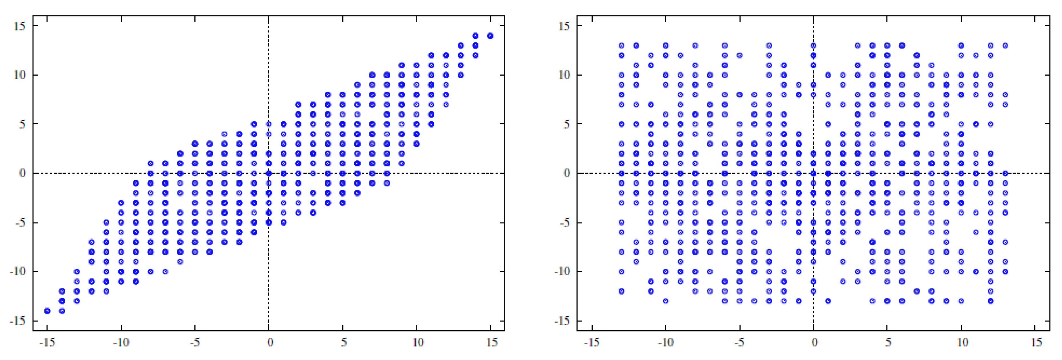
7.4. A Small Density Comparison with Ideal Lattices

Using an ideal lattice as a noise reduce the available set of secret keys drastically. The main point of ideal lattices is to reduce the size of the public key and the computation costs. In that regard, given a principal ideal lattice $\mathcal{L}(p,f)$, f should be public for efficient computations to be available. $p^{i}modf$ by iterating over i should give the rest of the noise beyond the first vector. Assuming f is anti-cyclic, or chosen in a way where $p^{i}modf$ has a taxicab norm lower than some constant D for all i, then the noise structure is decided by the choice of the first vector p.

Basically, compared to an ideal lattice, we pick $n-1$ more vectors randomly. Which means that while the choice for p is at most $\parallel V_n\parallel$ possibilities, our noise set has a factor $\parallel V_n{\parallel }^{n-1}$ over ideal lattices. $V_n$ being a set that grows more than exponentially as n increase, we can safely assume our noise set has a higher density than ideal lattices. It is unclear, however, if the density is exponentially vanishing for a fixed determinant as it is the case of ideal lattices: We do not know how to fix the determinant of a newly sampled DRS lattice.

Nevertheless, we believe it is safe to claim that the structure used here is safer than the structure provided by ideal lattices which are currently quite popular. Our reasoning should also apply for module lattices in a lesser extent (but with a similar asymptotic scale).

8. Conclusions and Open Questions

We presented in this paper a new method to generate secret keys for the DRS scheme, providing experimental results on the statistical distribution of the keys generated. We demonstrate that our new approach is sufficient to improve DRS to be secure against machine learning attacks as reported earlier in the literature. However, the secret matrix is still diagonal dominant and it remains an open question whether there exists a tight security proof to a well-known problem or if there is any unforeseen weaknesses to diagonal dominant lattices as both Li, Liu, Nitaj and Pan’s [17] and Yu and Ducas’s attacks [16] could lead to. The open questions for improvement stated in the original DRS report are also still applicable to our proposed iteration. Overall, we showed that both efficiency and security of such schemes are related to the noise more than the diagonal coefficients. Given a fixed diagonal, [16,17] showed weakness on particular noise sets. It is unclear if our choice of uniform sampling in the n-dimensional ball is provably secure, but we stress that the literature is very scarce concerning this lattice family and thus lots of open questions remain.

On the technical side, our method to generate random samples is also slow and might need improvement. It also impacts the setup as mentioned earlier, as keeping the current DRS parameters one can see the possibility to overflow and go over 64 bits, even though the probability is extremely low; thus, changing the public key generation is also left as an open question. The initial DRS scheme was very conservative not only on their security but also the manipulated integer size bounds: One might use heuristics to drastically increase the memory efficiency of the scheme and allow some small error probability, for example.

References

1. NIST. NIST Kicks Off Effort to Defend Encrypted Data From Quantum Computer Threat; NIST: Gaithersburg, MI, USA, 2016.
2. Shor, P.W. Polynomial-Time Algorithms for Prime Factorization and Discrete Logarithms on a Quantum Computer. Siam J. Comput. 1997, 26, 1484–1509. [Google Scholar] [CrossRef] [Green Version]
3. Minkowski, H. Geometrie der Zahlen; B.G. Teubner: Leipzig, Germany, 1896. [Google Scholar]
4. Ajtai, M. Generating hard instances of lattice problems. In Proceedings of the Twenty-Eighth Annual ACM Symposium on Theory of Computing; ACM: New York, NY, USA, 1996; pp. 99–108. [Google Scholar]
5. Goldreich, O.; Goldwasser, S.; Halevi, S. Public-key cryptosystems from lattice reduction problems. In Proceedings of the Annual International Cryptology Conference; Springer: Berlin, Germany, 1997; pp. 112–131. [Google Scholar]
6. Nguyen, P. Cryptanalysis of the Goldreich-Goldwasser-Halevi cryptosystem from crypto’97. In Proceedings of the Annual International Cryptology Conference; Springer: Berlin, Germany, 1999; pp. 288–304. [Google Scholar]
7. Fischlin, R.; Seifert, J.P. Tensor-based trapdoors for CVP and their application to public key cryptography. In Cryptography and Coding; Springer: Berlin, Germany, 1999; pp. 244–257. [Google Scholar]
8. Micciancio, D. Improving lattice based cryptosystems using the Hermite normal form. In Cryptography and Lattices; Springer: Berlin, Germany, 2001; pp. 126–145. [Google Scholar]
9. Paeng, S.H.; Jung, B.E.; Ha, K.C. A lattice based public key cryptosystem using polynomial representations. In International Workshop on Public Key Cryptography; Springer: Berlin, Germany, 2003; pp. 292–308. [Google Scholar]
10. Sloane, N.J.A. Encrypting by Random Rotations. In Cryptography, Proceedings of the Workshop on Cryptography Burg Feuerstein, Germany, 29 March–2 April 1982; Beth, T., Ed.; Springer: Berlin/Heidelberg, Germany, 1983; pp. 71–128. [Google Scholar]
11. Regev, O. New lattice-based cryptographic constructions. J. ACM 2004, 51, 899–942. [Google Scholar] [CrossRef]
12. Gama, N.; Izabachene, M.; Nguyen, P.Q.; Xie, X. Structural lattice reduction: Generalized worst-case to average-case reductions and homomorphic cryptosystems. In Annual International Conference on the Theory and Applications of Cryptographic Techniques; Springer: Berlin/Heidelberg, Germany, 2016; pp. 528–558. [Google Scholar]
13. NIST. Post-Quantum Cryptography Standardization; NIST: Gaithersburg, MI, USA, 2018.
14. Plantard, T.; Sipasseuth, A.; Dumondelle, C.; Susilo, W. DRS: Diagonal Dominant Reduction for Lattice-Based Signature. PQC Standardization Process, Round 1 Submissions. 2018. Available online: https://csrc.nist.gov/Projects/Post-Quantum-Cryptography/Round-1-Submissions (accessed on 15 May 2019).
15. Plantard, T.; Susilo, W.; Win, K.T. A digital signature scheme based on CVP max. In InInternational Workshop on Public Key Cryptography; Springer: Berlin/Heidelberg, Germany, 2008; pp. 288–307. [Google Scholar]
16. Yu, Y.; Ducas, L. Learning Strikes Again: The Case of the DRS Signature Scheme. In Proceedings of the International Conference on the Theory and Application of Cryptology and Information Security, Brisbane, Australia, 2–6 December 2018; pp. 525–543. [Google Scholar]
17. Li, H.; Liu, R.; Nitaj, A.; Pan, Y. Cryptanalysis of the randomized version of a lattice-based signature scheme from PKC’08. In Proceedings of the Australasian Conference on Information Security and Privacy; Springer: Berlin/Heidelberg, Germany, 2018; pp. 455–466. [Google Scholar]
18. Brualdi, R.A.; Ryser, H.J. Combinatorial Matrix Theory; Cambridge University Press: Cambridge, UK, 1991; Volume 39. [Google Scholar]
19. Wei, W.; Liu, M.; Wang, X. Finding shortest lattice vectors in the presence of gaps. In Proceedings of the Cryptographers’ Track at the RSA Conference, San Francisco, CA, USA, 20–24 April 2015; Springer: Berlin/Heidelberg, Germany, 2015; pp. 239–257. [Google Scholar]
20. Ajtai, M.; Dwork, C. A public-key cryptosystem with worst-case/average-case equivalence. In Proceedings of the Twenty-Ninth Annual ACM Symposium on Theory of Computing; ACM: New York, NY, USA, 1997; pp. 284–293. [Google Scholar]
21. Gama, N.; Nguyen, P.Q. Predicting lattice reduction. In Proceedings of the Annual International Conference on the Theory and Applications of Cryptographic Techniques; Springer: Berlin/Heidelberg, Germany, 2008; pp. 31–51. [Google Scholar]
22. Liu, M.; Wang, X.; Xu, G.; Zheng, X. Shortest Lattice Vectors in the Presence of Gaps. IACR Cryptol. Eprint Arch. 2011, 2011, 139. [Google Scholar]
23. Lyubashevsky, V.; Micciancio, D. On bounded distance decoding, unique shortest vectors, and the minimum distance problem. In CRYPTO 2009; Springer: Berlin/Heidelberg, Germany, 2009; pp. 577–594. [Google Scholar]
24. Babai, L. On Lovász’ lattice reduction and the nearest lattice point problem. Combinatorica 1986, 6, 1–13. [Google Scholar] [CrossRef]
25. Bajard, J.C.; Imbert, L.; Plantard, T. Modular number systems: Beyond the Mersenne family. In International Workshop on Selected Areas in Cryptography; Springer: Berlin/Heidelberg, Germany, 2004; pp. 159–169. [Google Scholar]
26. Plantard, T. Arithmétique modulaire pour la cryptographie. Ph.D. Thesis, 2005. Available online: https://documents.uow.edu.au/~thomaspl/pdf/Plantard05.pdf (accessed on 15 May 2019).
27. Nguyen, P.Q.; Regev, O. Learning a parallelepiped: Cryptanalysis of GGH and NTRU signatures. J. Cryptol. 2009, 22, 139–160. [Google Scholar] [CrossRef]
28. Ducas, L.; Nguyen, P.Q. Learning a zonotope and more: Cryptanalysis of NTRUSign countermeasures. In International Conference on the Theory and Application of Cryptology and Information Security; Springer: Berlin/Heidelberg, Germany, 2012; pp. 433–450. [Google Scholar]
29. Gentry, C.; Peikert, C.; Vaikuntanathan, V. Trapdoors for hard lattices and new cryptographic constructions. In STOC 2008; ACM: New York, NY, USA, 2008; pp. 197–206. [Google Scholar]
30. Pernet, C.; Stein, W. Fast computation of Hermite normal forms of random integer matrices. J. Number Theory 2010, 130, 1675–1683. [Google Scholar] [CrossRef] [Green Version]
31. Serra-Sagristà, J. Enumeration of lattice points in l1 norm. Inf. Process. Lett. 2000, 76, 39–44. [Google Scholar] [CrossRef]
32. Smith, N.A.; Tromble, R.W. Sampling Uniformly From the Unit Simplex; Johns Hopkins University: Baltimore, MD, USA, 2004. [Google Scholar]
33. Knuth, D.E.; Graham, R.L.; Patashnik, O.; Liu, S. Concrete Mathematics; Adison Wesley: Boston, MA, USA, 1989. [Google Scholar]
34. Derzko, N.; Pfeffer, A. Bounds for the spectral radius of a matrix. Math. Comput. 1965, 19, 62–67. [Google Scholar] [CrossRef]
35. Wilkinson, J.H. The Algebraic Eigenvalue Problem; Clarendon: Oxford, UK, 1965; Volume 662. [Google Scholar]
36. Bartels, R.H.; Stewart, G.W. Solution of the matrix equation AX+ XB= C [F4]. Commun. ACM 1972, 15, 820–826. [Google Scholar] [CrossRef]
37. Golub, G.; Nash, S.; Van Loan, C. A Hessenberg-Schur method for the problem AX+ XB= C. IEEE Trans. Autom. Control 1979, 24, 909–913. [Google Scholar] [CrossRef] [Green Version]
38. Householder, A.S. The Theory of Matrices in Numerical Analysis; Courier Corporation: Chelmsford, MA, USA, 1964. [Google Scholar]
39. Kannan, R. Minkowski’s convex body theorem and integer programming. Math. Oper. Res. 1987, 12, 415–440. [Google Scholar] [CrossRef]
40. Van de Pol, J.; Smart, N.P. Estimating key sizes for high dimensional lattice-based systems. In Proceedings of the IMA International Conference on Cryptography and Coding; Springer: Berlin/Heidelberg, Germany, 2013; pp. 290–303. [Google Scholar]
41. Hoffstein, J.; Pipher, J.; Schanck, J.M.; Silverman, J.H.; Whyte, W.; Zhang, Z. Choosing parameters for NTRUEncrypt. In Proceedings of the Cryptographers’ Track at the RSA Conference; Springer: Cham, Switzerland, 2017; pp. 3–18. [Google Scholar]
42. Chen, Y.; Nguyen, P.Q. BKZ 2.0: Better lattice security estimates. In Proceedings of the InInternational Conference on the Theory and Application of Cryptology and Information Security; Springer: Berlin/Heidelberg, Germany, 2011; pp. 1–20. [Google Scholar]
43. The FPLLL Team. FPLLL, a Lattice Reduction Library. Available online: https://github.com/fplll/fplll (accessed on 15 May 2019).
44. Sipasseuth, A.; Plantard, T.; Susilo, W. Improving the security of the DRS scheme with uniformly chosen random noise. In Proceedings of the Australasian Conference on Information Security and Privacy; Springer: Cham, Switzerland, 2019. [Google Scholar]
45. Computational Algebra Group. U.o.S. 2018. Available online: https://magma.maths.usyd.edu.au/calc/ (accessed on 15 May 2019).
46. PARI Group. U.o.B. PARI-GP. 2018. Available online: https://pari.math.u-bordeaux.fr/gp.html (accessed on 15 May 2019).
Figure 1. Signatures over l 2 and l .
Information 11 00133 g001
Figure 2. Figures in the second row show the regions to which ( w i , w j ) in two cap regions will be moved by reduction at index i when S i , j = b , 0 , b , respectively, from left to right.
Information 11 00133 g002
Figure 3. Example output where the DRS bound fails but the PSW bound passes
Information 11 00133 g003
Figure 4. Example output where the PSW bound fails but the DRS bound passes
Information 11 00133 g004
Figure 5. f ( v ) distribution for n = 1108 , 1372 , 1779 and D = n 1 over 10 6 samples.
Information 11 00133 g005
Figure 6. Percentage of key recoveries of BKZ20 (20 sample keys/dim).
Information 11 00133 g006