A Generic WebLab Control Tuning Experience Using the Ball and Beam Process and Multiobjective Optimization Approach

Abstract

In control engineering education, the possibility of using a real control system in the learning process motivates professors to improve both students’ knowledge and skills, thus avoiding an approach only based on control theory. While considering that control engineering laboratories are expensive, mainly because educational plants should reproduce classical problems that are found in the industry, the use of virtual laboratories appears as an interesting strategy for reducing costs and improving the diversity of experiments. In this research, remote experimentation was assumed regarding the ball and beam process as an alternative didactic methodology. While assuming a nonlinear and unstable open-loop process, this study presents how students should proceed to control the plant focusing on the topic that is associated with multiobjective optimization. Proportional-Integral-Derivative (PID) controller was tuned considering the Non-dominated Sorting Genetic Algorithm (NSGA-II) to illustrate the WebLab learning procedures described in this research. The proposed strategy was compared to the Åström’s robust loop shaping method to emphasize the performance of the multiobjective optimization technique. Analyzing the feedback provided by the students, remote experimentation can be seen as an interesting approach for the future of engineering learning, once it can be directly associated with industry demand of connected machines and real-time information analysis.

1. Introduction

The control engineering is an area of study where scientific and technological development supports the quality improvement of process and products, thus guarantying repeatability and precision in industrial applications. In this context, automatic control can be considered to be essential in many fields of science and engineering [1], e.g., electronics, chemistry, robotics, manufacturing systems, etc. The two main difficulties that are presented in [2] are related to the educational process that is associated with automatic control, the first one consists in understanding how to draft control systems, and the second is how to associate mathematical results to practical problems.

Active learning methodologies are being used in many areas, and digital media associated with learning activities seem to increase both students’ knowledge and skills [3]. The main idea is to provide a more efficient and faster learning way to assimilate knowledge while considering distinct strategies to hold students’ attention, like simulations, videos, and interactive experiments [4].

This work starts presenting some successful approaches, including digital media in the learning process. The first one was in the health care area [5], where interesting results were obtained using gamification to improve the competences and knowledge while considering a non-traditional training source for caregivers of people with dementia. The authors reported that the game provoked positive attitudes for future caregivers when compared to traditional methods, providing a more relaxed behavior, decreasing fear during the caring process.

While considering that working memory is an essential function for human cognition, in the work presented in [6], it was assumed that robotics and artificial intelligence (AI) would develop a novel system for training human memory based on three aspects: working memory stimulation by remembering visual sequences; development of an intelligent agent for decision-making; and, a fuzzy controller to generate customized levels according to the user. The experimental results showed significant improvement of user’s performance in the presented game, which could be related to improvements that are associated with their working memory.

In the electrical engineering area, a remote-controlled experiment focusing on power electronics was proposed as a virtual laboratory experiment [7]. The main idea is that students can configure parameter controls, connect wires, and test distinct electric load conditions with predefined electronic laboratory instruction. The authors reported that students presented better time management, and improved their learning and understanding of laboratory procedures when compared to traditional laboratory classes.

The use of WebLabs in engineering education provides an alternative option to the inclusion of laboratory experiments during the teaching process. In this approach, teaching laboratories are available on an online platform, where the students can perform their experiments at any time. In this case, laboratory resources can be shared with other institutions, ensuring the diversity of experiments, even in remote locations [8].

Motivated by the results that were obtained in the previously mentioned works, especially the one assuming AI, distance-learning applications are growing fast, especially those that were associated with WebLabs or virtual laboratories. In engineering education, innovative experiments can be used to help students increase practical knowledge in a faster and easier way, developing skills that will be important during their professional activities. However, an ideal infrastructure is not always available. In this way, it is important to solve this issue to guarantee excellence in the learning process [9]. WebLabs can be used to solve the problem that is associated with the variability in infrastructure by sharing laboratory resources among students. Moreover, industries are also considering WebLab during training activities, reducing the learning time and providing a remote evaluation of processes focusing on cost reduction [10].

1.1. Control Engineering Learning Involving the Ball and Beam Process

In the control systems engineering area, students should develop autonomy to solve practical problems that were found in the industry, e.g., fluid level or flow control, temperature regulation, pressure control, among others. In the work that is presented in [11], a machine learning-based system that uses a game formulation for engineering collaboration to develop autonomy in control engineering was presented. While taking into account that remote control systems are in evidence in both academic and industrial areas [12], educational processes can be used to replicate complex systems that are frequently found in the industry. One of these is the ball and beam process, which is a nonlinear open-loop unstable system. The main objective is to control the position of a ball on a beam while considering a variable beam angle. This process, for example, can be used to study the control problem associated with the horizontal stabilization of an airplane [13].

The literature review that is presented in the sequence of this article is focused on studies concerning the ball and beam process to emphasize its importance during control engineering learning. Section 1.1.1 describes studies considering the modeling and simulation of the ball and beam process. Focusing on a more practical approach, some researches adopted the construction of the ball and beam plant in order to avoid just modeling and simulation. In this case, the literature review presented in Section 1.1.2 addressed some studies that considered the construction of the process.

1.1.1. Related Works Associated with the Ball and Beam Modeling and Simulation

The present subsection addresses some works that involve the simulation of control strategies for the ball and beam plant. In the study that is presented in [14], the ball and beam model was used to test a nonlinear control strategy based on input-output linearization. In this case, it was presented that a standard Jacobian linearization fails in controlling the ball and beam system. The study presented that it is possible to control the process based on an approximate input-output linearization idea. Following a similar linearization approach, in [15] a robust feedback linearization to solve the ball and beam control problem was presented. In this case, an outer-loop linear controller was addressed based on the $\mu$-synthesis technique. Finally, robust stability results were obtained through computer simulations of the ball and beam plant.

Ref. [16] presents an association between the sliding-model control and fuzzy control. In this case, the system was divided into two second-order transfer functions and, in each subsystem, it was considered to be a separate control target to each model, those expressed in terms of sliding surfaces. Additionally, the ball and beam system was assumed as one of the three cases selected to evaluate the proposed control strategy. The hybrid strategy showed a reduction in the number of fuzzy rules, thus reducing the complexity of the controller.

Another simulation-based approach considering a similar structure to the one that is presented in this article, but while assuming mono-objective optimization, was presented in [17], where a Proportional Integral-Derivative (PI-D) and a Proportional Integral-Proportional Derivative (PI-PD) controllers were tuned while using Simulated Annealing (SA) and Cuckoo Search Algorithm (CSA). An active disturbance rejection control (ADRC) strategy was presented in [18] to conclude the first part of this literature review. The controller consists of a tracking differentiator (TD), an extended state observer (ESO), a nonlinear state error feedback control law (NLSEF), and a disturbance compensation device (DCD). The ADRC was compared with a classical Proportional-Integral-Derivative (PID) controller showing promising results in terms of the percentage overshoot after reference variations. Additionally, improvements in speed when compared to the traditional PID control strategy were obtained.

1.1.2. Related Works Associated with the Construction of the Ball and Beam Plant

The works that are presented in this subsection constitute the second part of the literature review. Here, works focusing on the construction of a physical plant for the ball and beam process are described.

During simulations, disturbances do not affect the behavior of the system. On the other hand, when a real plant is considered, it is possible to evaluate problems that are associated with the network during communication, additional dynamics as transport delay, noisy signals, among other effects that are associated with the control of real systems. One example is the work that is presented in [19], where an apparatus was used during tests of both static and dynamic Sliding Mode Control (SMC) schemes. Additionally, four approaches assuming two modeling strategies, one simplified and other complete, were considered. The results showed that when the complete model was assumed, improved performance for controlling the ball position was obtained, mainly when the dynamic controller was considered.

An experimental approach was performed in [20], where the developed ball and beam apparatus was associated with a Linear Quadratic Regulator (LQR) controller. The main idea was to both stabilize and control the system by changing poles to optimal locations. While assuming a genetic algorithm to determine the optimal LQR configuration, two approaches were considered during the tests. The first one assumed a model-based configuration, while the second one considered a non-model-based controller. Both of the approaches used the PID controller and its variations, and the LQR strategy. The results showed that the LQR model-based approach provided better results when the steady-state error was evaluated.

Another ball and beam apparatus was presented in [21], where a Takashi-Sugeno fuzzy model-based adaptive dynamic surface controller was proposed. The proposed controller was compared to the conventional Dynamic Surface Control (DSC) strategy. The results showed that superior performance was obtained by the fuzzy approach in terms of computation robustness and feasibility. Other work considering a fuzzy controller was addressed in [22], but, in this case, real-time tuning was the objective of the study. Assuming the Differential Evolution (DE) algorithm [23], the possibility of real-time tuning while considering a classical PID structure was presented.

The association between the ball and beam plant and WebLabs can be found in [13]. This work was developed with the purpose of helping students of control engineering during their activities associated with advanced control theory. In this sense, students could compare the performance of their controllers with classical and well-established strategies. The WebLab system was developed, associating Easy Java Simulations (EJS) and Moodle learning management systems.

A state feedback LQR based control scheme, which consists of Linear Quadratic Estimator (LQE) and LQR, was presented in [24], to conclude this literature review section of this article. The ball position was considered the output, where all system states were calculated using both the ball position and its time derivatives. Additionally, the ball and beam apparatus was built while considering a servo motor used to modify the beam angle and a potentiometer to measure the ball position.

The literature review that is presented in the first part of this article showed that distinct control strategies can be associated with the ball and beam control problem. However, just a few works considered virtual experimentation as the one assumed in the present study. The research question associated with this work can be stated based on this statement. Is it possible to propose an interesting approach directed to advanced control learning, which is capable of reaching as many students as possible that are focused on learning through practical experiments, even considering a limited laboratory structure?

Previous works showed that the ball and beam process became a benchmark for testing different control strategies, showing to be an important process in control engineering learning. By associating virtual laboratories and control engineering, this article presents a WebLab approach for advanced control learning to make the most of the didactical processes available at the university, in order to reach as many students as possible. We considered the ball and beam process as a case study to illustrate all the procedures that should be performed by the students. The methodology consists of the development of advanced control strategies for the process using multiobjective optimization. While considering a wide range of algorithms available for this purpose, we have described all of the procedures using the Non-dominated Sorting Genetic Algorithm (NSGA-II). Finally, students that participate in the control WebLab experience could deal with distinct software, such as LabView and MATLAB, Python programming, among others, verifying the importance of system integration for remote data acquisition and control.

The next section of this article presents the ball and beam apparatus adopted in this study focusing on process modeling procedures. Section 3 presents the theoretical basis of PID control. Section 4 addresses the procedures to apply multiobjective optimization in control problems. When the classical PID control action is assumed, then the procedures to use evolutionary multiobjective optimization (EMO) algorithms to tune the controller are based on three steps: the definition of the multiobjective problem, the multiobjective optimization routine, and the multicriteria decision making. All of the previously mentioned steps are addressed in Section 4. Section 5 presents the experimental routine considering the ball and beam apparatus. Section 6 describes the Non-dominated Sorting Genetic Algorithm (NSGA-II), which is the algorithm that is assumed in this study. In the same section, the results that were obtained using NSGA-II were compared with Åström’s robust loop shaping method to show the advantages of the multiobjective approach. Finally, Section 7 presents the conclusions and future works that are associated with this research.

2. Ball and Beam Process Description and Modelling

This section presents the ball and beam apparatus used during the development of this research, as well as two modeling approaches that were assumed to obtain the process model.

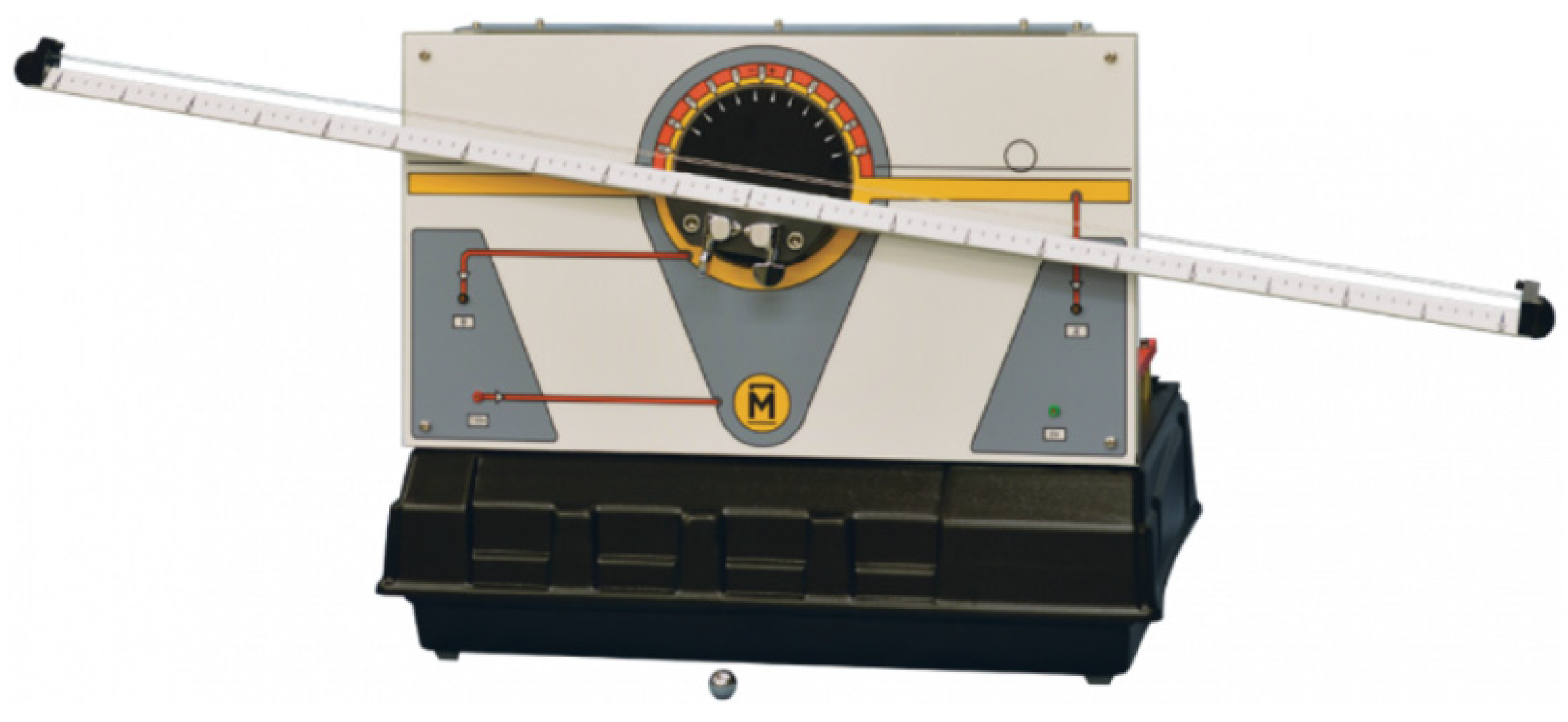
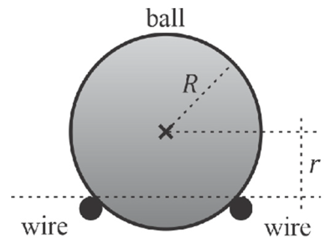
2.1. The Ball and Beam Apparatus

While considering that different hardware implementations may cause differences in the dynamic of the plant, which are mainly due to variations on both mechanical and electrical architectures, the coefficients of the transfer function that are associated with each plant could change [1]. In this way, this section describes the plant that is adopted in this research. The ball and beam apparatus corresponds to the CE 106 from Tecquipment [25] (see Figure 1), which was developed to be an educational plant in learning activities that is associated with control engineering.

The process that was adopted in this study is based on a beam that can rotate through an angle of $\pm 10$°. The input signal represents the motor input voltage ($0$ to $+10$ VDC), and two outputs are available (0 to $\pm 10$ VDC): the ball position and the beam angle, respectively. When a signal is applied to the motor input, it varies the speed of the motor. A profiled cam, which is attached to the motor shaft, links the main beam via a secondary one. Additionally, a potentiometer allows for measuring the voltage that is associated with the beam angle. Two parallel wires are stretched along the top of the beam, where the ball may roll, to measure the ball position. When the ball rests between the wires, it allows for a fraction of the source voltage to be measured at the other wire while using a potentiometer.

There is no fixed point in the beam extremity, just in the center. It is possible to consider two modeling approaches, one that is based on a simplified formulation and a second one based on a complete formulation. Both of the models are presented in the sequence of this work.

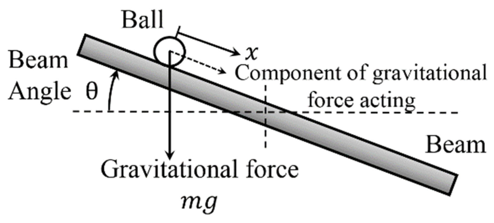
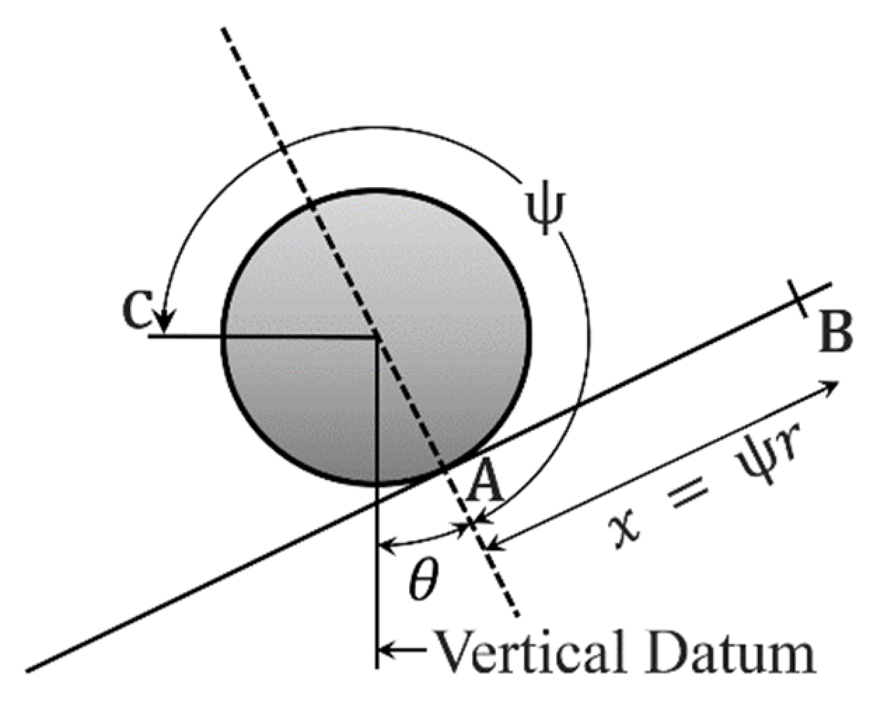
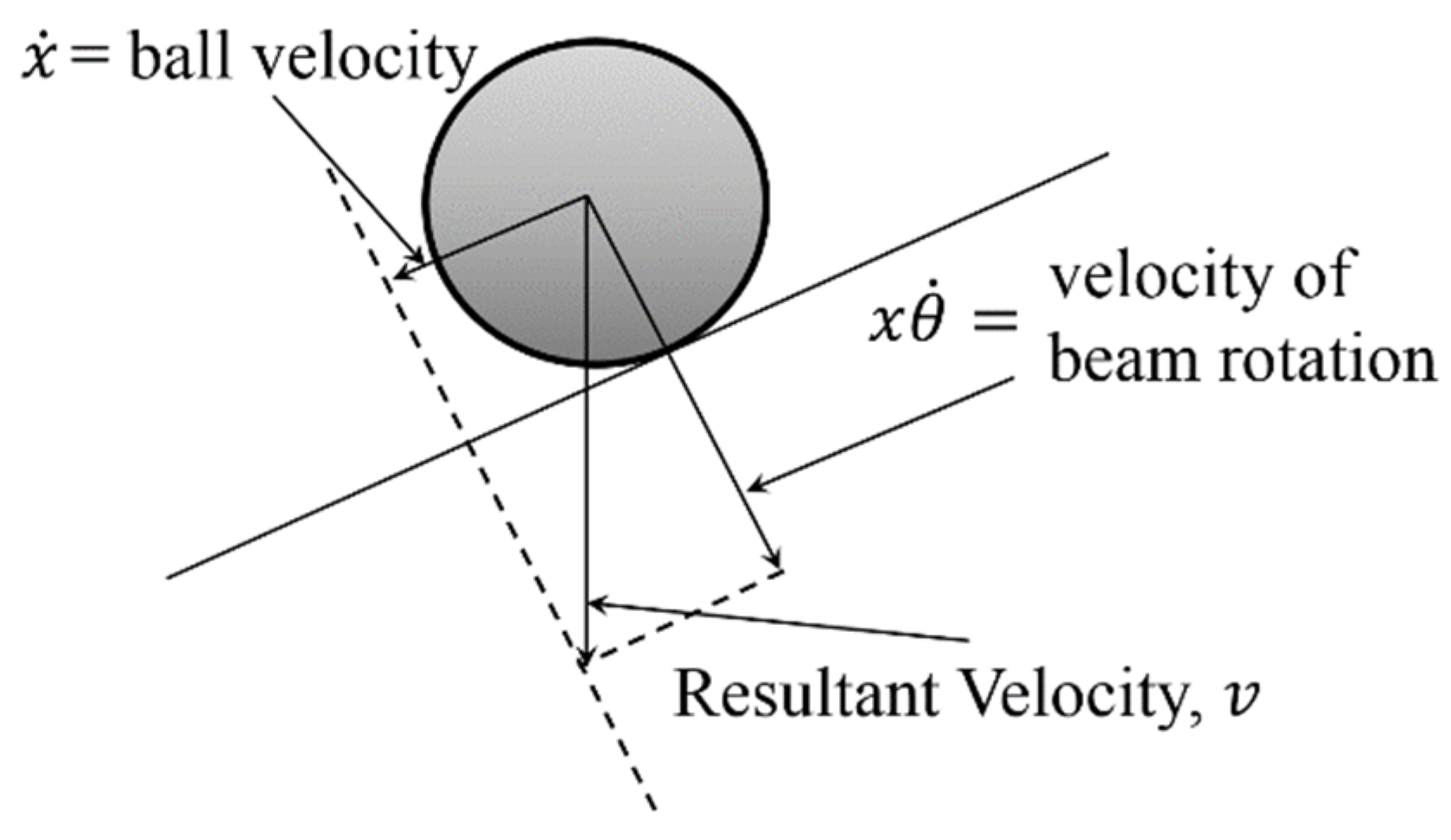
2.2. Physical Modeling

This subsection describes the two modeling methods of the ball and beam process to obtain the simplified model or the full model, which can be used as parametric models for system simulation.

2.2.1. Simplified Model

The modeling process starts with the dynamic of the ball when rolling on the beam. While assuming the force, which accelerates the ball as it rolls, the component can be formulated based on the gravitational force, see Figure 2.

The simplified model considers no friction during the ball sliding over the beam. In this way, the mathematical equation that describes the movement is

$$mg\sin \theta =m\ddot{x}.$$

(1)

When small angles are considered, $\sin \theta =\theta .$ Finally, the transfer function of the plant relates the beam angle, $\theta$, and the ball position, $x$, as presented in Equation (2).

$$\frac{X\left(s\right)}{\Theta \left(s\right)}=\frac{g}{s^2}.$$

(2)

2.2.2. Full Model

The full model can be obtained while considering the Lagrangian method, where the Lagrangian, $L$, for the process can be stated as

$$L=U^{*}-T,$$

(3)

In Equation (3), $U^{*}$ represents the kinetic energy and $T$ is the potential energy in the system. When an open-loop equation is considered, the potential energy becomes zero, since there are no springs in the system. The potential energy that is provided by the gravity is considered and the Lagrangian is given by the kinetic energy, which represents both the translational and the rotational kinetic energy of the ball.

$$L=U^{*}=\frac{1}{2}m{v}^2+\frac{1}{2}I{\omega }^2$$

(4)

where $m$ is the ball mass and $I$ is the ball moment of inertia. The translational velocity of the ball, $v$, and the angular velocity of the ball, $\omega$, have to be re-written in terms of the generalized coordinates $x$ and $\theta$ to obtain the transfer function. While considering an angular distance $x$, which was rolled by the ball, the angular velocity $\omega$ can be obtained, see Figure 3. In this case, $r$ represents the rolling radius of the ball.

$$\omega =\frac{\dot{x}}{r}+\dot{\theta }.$$

(5)

Figure 4 presents the velocity $v$ of the ball can be obtained from the velocity diagram.

$$v^2={(\dot{x})}^2+{(x\dot{\theta })}^2,$$

(6)

While considering the angular velocity that is presented in Equation (5), and the resultant velocity of Equation (6), the Lagrangian of Equation (4) can be re-written, as presented in Equation (7), while the moment of inertia of the ball is presented in Equation (8).

$$L=\frac{1}{2}m\left({(\dot{x})}^2+{(x\dot{\theta })}^2\right)+\frac{1}{2}I{\left(\frac{\dot{x}}{r}+\dot{\theta }\right)}^2,$$

(7)

$$I=\frac{2}{5}m{R}^2$$

(8)

where $R$ represents the ball radius. While considering that the ball rest between two wires, the radius $R$ is always larger than the rolling radius $r$, see Figure 5.

Finally, the model of the system can be obtained based on the Lagrangian equation.

$$\frac{d}{dt}\left(\frac{\delta L}{\delta \dot{x}}\right)-\frac{\delta L}{\delta x}=mg\sin \theta .$$

(9)

The complete model of the ball and beam process, which associates the radius $R$, the rolling radius, $r$, the beam angle, $\theta$, the ball position, $x$, and the gravitational acceleration, $g$, can be expressed by:

$$\frac{d}{dt}\left(\frac{\delta L}{\delta \dot{x}}\right)-\frac{\delta L}{\delta x}=mg\sin \theta .$$

(10)

Equation (10) represents a nonlinear model, as it involves a nonlinear term that associates both the beam velocity and its angle, and the ball position. In this case, the model must be linearized while considering small-angle variations to obtain an approximated linear system. Moreover, the velocity of the beam and its acceleration are also both considered to be small. In this way, the transfer function of the ball and beam process can be obtained while considering the full formulation associating the ball position (output of the system), and the beam angle (input of the system), see Equation (11).

$$\frac{X\left(s\right)}{\Theta \left(s\right)}=\frac{g}{\left(1+\frac{2R^2}{5r^2}\right)s^2}.$$

(11)

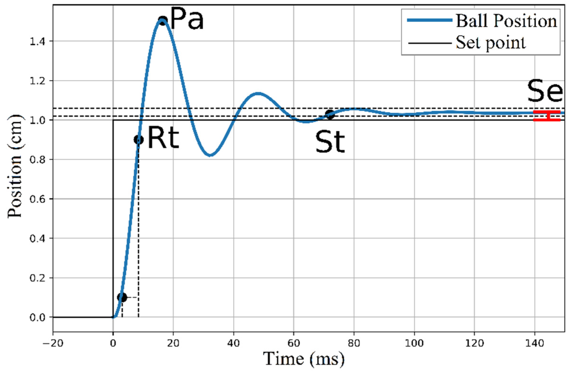
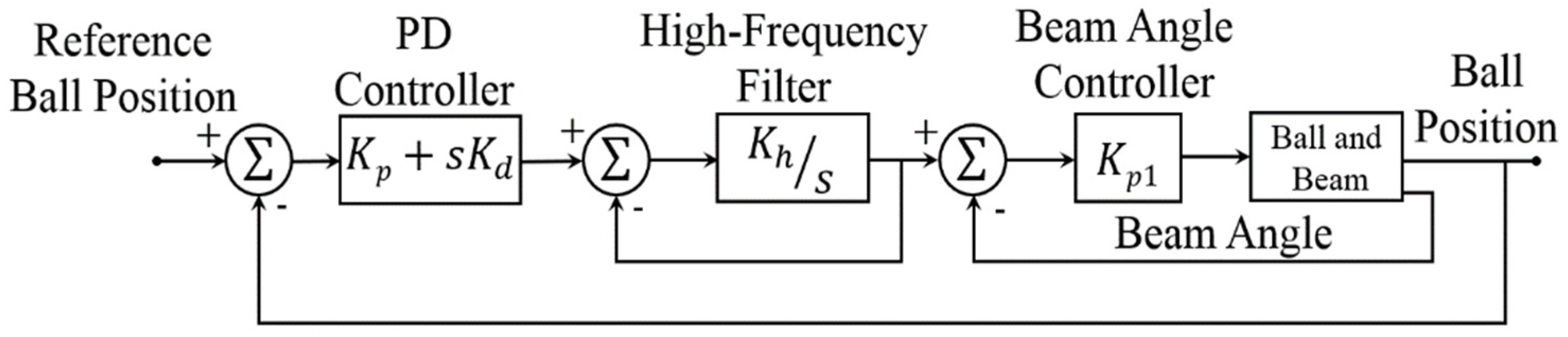
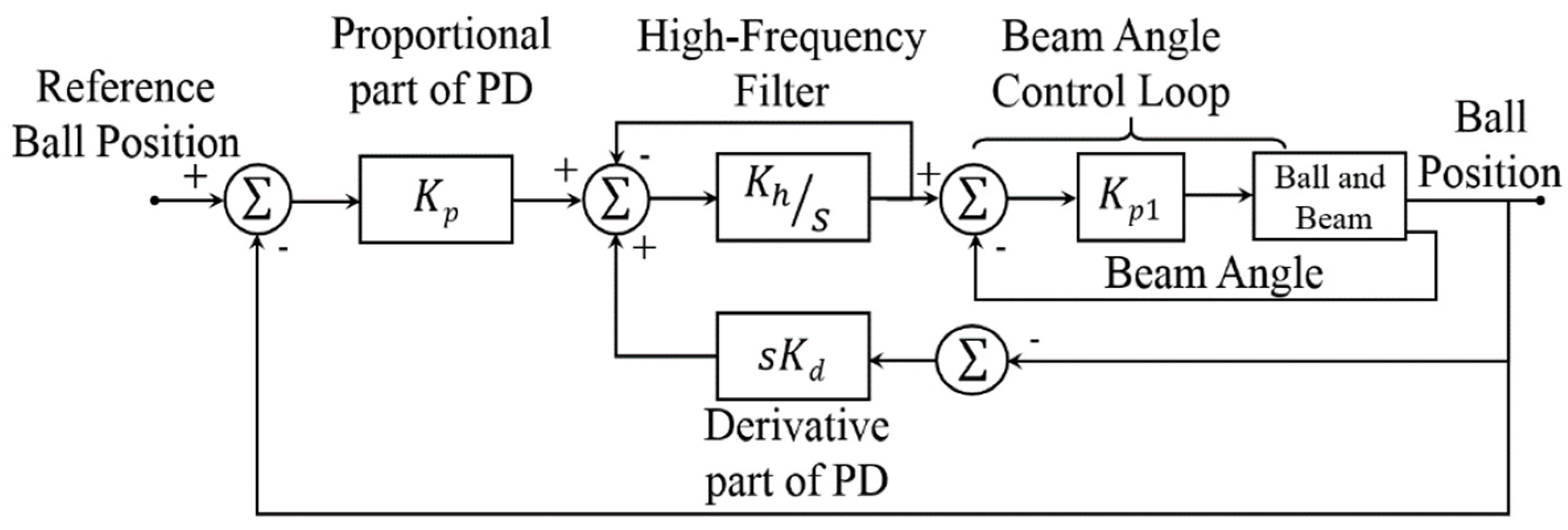
3. PID Control and Performance Measures

Proportional-Integral-Derivative (PID) controllers are used in 90% of control applications [26], as reported by the Japan Electric Measuring Instrument Manufacturers’ Association. The main motivation to be considered is that other approaches often need mathematical models as a state-space representation or transfer functions to be formalized, short implementation time, and when the implementation effort is evaluated, other techniques frequently present small advantages over the PID controllers [27].

The classical PID controller transfer function, $C\left(s\right)$, can be defined based on three gains: the proportional gain, $K_p$, the derivative gain, $K_d$, which can be associated with the derivative time, $T_d$, and the integral gain, $K_i$, which can be associated with the integral time, $T_i$.

$$C\left(s\right)=K_p+\frac{K_i}{s}+K_{d}s=K_p\left(1+\frac{1}{T_{i}s}+T_{d}s\right).$$

(12)

Frequently, one of the most common objectives in control systems is to reduce the errors between the reference and the system output in a shorter time [18,24]. In the case of the ball and beam system, the objective is to control the ball position that is based on an error signal,$e\left(t\right)$, which represents the difference between the desired ball position and the real ball position. A classical PID work on the error signal, which is processed to generate a control signal. These procedures form an iterative process until the stabilization of the ball on the desired position.

In control systems, the analysis of the response of the system over time consists of two sections: the transient response and the steady-state response. The first one is related to a change in the reference of the system, the response goes from the initial to a final state. Performance metrics can be assumed to evaluate the transient response of the system, such as the rise time ($Rt$); the time spent by the system to reduce the output error from 90% to 10%; the peak amplitude or overshoot ($Pa$), which is the maximum value reached by the system response caused by a reference change; and, the settling time ($St$), representing the time that is taken for the error to be reduced to a value smaller than 2% or 5%. The second one, or the steady-state response, refers to the output system behavior is stabilized, i.e., when the system do not present an oscillatory behavior or the time approaches to infinity, in this situation the stationary error ($Se$), which indicates the percentage error after output stabilization, can be evaluated [1]. Figure 6 illustrates the previously mentioned performance coefficients for a second-order system step response, where a change in the reference is performed and the system presents an oscillatory behavior until the stabilization, more information regarding the previously mentioned performance measures can be found in [1].

The PID control system has block diagram variations that can be found in the literature [28]. Some of them are the PI-D (Figure 7a) and Integral-Proportional Derivative (I-PD) (Figure 7b). The PI-D variation has the derivative portion removed from the forward branch and placed on the feedback branch. The forward branch corresponds to the direct way between the input and the output of the system. The feedback branch corresponds to a measure of the output signal that is used to calculate the error between the reference and the real system’s output. This modification results in a control strategy where the derivative term acts on the plant output signal $y\left(t\right)$, not in the difference $x\left(t\right)-y\left(t\right)$. In this way, no differentiation is applied over $x\left(t\right)$ step input, because step differentiation would generate a high amplitude signal at the actuator, thus leading to sorter lifetime or damages. In other cases, PI-D is used to avoid the amplification of high-frequency noise that might be present in the reference or in the error signals.

Some metrics that are commonly used in experiments that are related to the error are the Integral Absolute Error ($IAE$) (13) and the Integral of Time multiplied by Absolute of the Error ($ITAE$) (14) to evaluate the controller’s performance. Related to the control effort, it can be cited the Integral of Time multiplied by the Squared Error ($ITSE$) (15) and the Integral of the Absolute Variation of Control Signal ($IAVU$) (16), where $u$ represents the control signal and $t$ is the current experiment time in seconds [29].

$$IAE={\displaystyle \int }\left|e\left(t\right)\right|dt$$

(13)

$$ITAE={\displaystyle \int }t\left|e\left(t\right)\right|dt$$

(14)

$$ITSE={\displaystyle \int }t{e}^2\left(t\right)dt$$

(15)

$$IAVU={\displaystyle \int }\left|\frac{du\left(t\right)}{dt}\right|dt$$

(16)

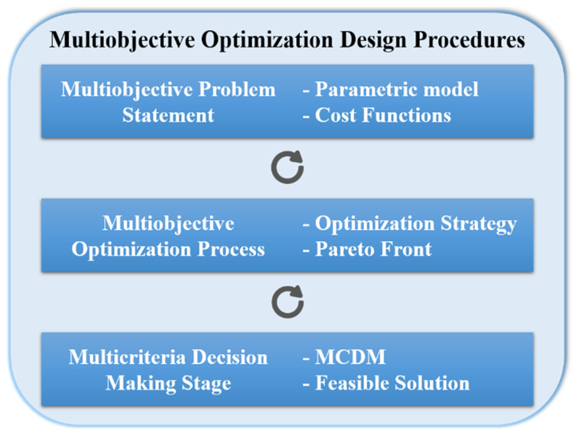
4. Multiobjective Optimization Applied to Control Engineering

When trying to solve an engineering problem, it is common to search for solutions that provide the best performance when compared to other possible solutions. This is the principle of an optimization problem, where a solution based on predetermined assessment conditions, which improves the system performance, is required [30].

Most of the engineering problems can be stated as optimization problems. When multiple objectives are considered, conflicting objectives often appear during the problem formulation. An example of this case was addressed in [31], where the authors focused on the improvement of the system performance, trying to avoid the increase of energy consumption.

Assuming the condition of conflicting objectives, some strategies can be stated in order to obtain a reasonable solution for the problem. Most of these strategies consist of aggregating multiple objectives in a single function, thus reducing the complexity of analyzing a set of solutions. Aggregating strategies have an articulation of preferences prior to the optimization process, e.g., by defining weighting factors among all of the objectives, where the solution will reflect the preferences of the decision-maker. Examples of the previously mentioned case are the weighted global criterion method, the weighted sum method, the lexicographic method, the weighted min-max method, and others (for a detailed description see [32]).

Some recent techniques that can be used to solve this kind of problems are the Jaya algorithm [33], the Proactive Particles in Swarm Optimization (PPSO) [34], the Hybrid Population-Based Mean-Variance Mapping Optimization (MVMO-PH) [35], the Successful-History based Adaptative Differential Evolution with Linear size reduction and four adaptation strategies with Improved ε constraint-handling method (LSHADE44-IEpsilon) [36], the Hunting Optimization (HO) [37], and the Modified Adaptative Bats Sonar Algorithm with Doppler Effect (MABSA-DE) [38].

Another approach for solving multiobjective optimization problems is though the simultaneous optimization of different objective functions. In this case, each objective function is treated as a distinct problem, and a set of solutions is obtained at the end of the optimization process. In this case, it is not necessary to normalize the cost functions, as the analysis and selection of a solution will be made a posteriori of the optimization process. Some of the newer techniques that can be used are the Bayesian Multi-Objective Optimization (BMOO) [39], the Adaptative Gradient Multiobjective Particle Swarm Optimization (AGMOPSO) [40], the Multiobjective Simulated Kalman Filter algorithm (MOSKF) [41], the Hybrid Multi-Objective Cuckoo Search (HMOCS) [42], among others.

The main difference between the two presented approaches is that the second one needs a multicriteria decision making (MCDM) strategy. In classical decision-making researches, it is common to find some formulations to aggregate multiple cost functions into a single objective function, where the focus is to select an optimal solution. The MCDM method evaluates the trade-offs of the candidate solutions to assess the contribution of each one for the problem, ranking them [43].

While considering MOPs in the control engineering area, the process of improving performance measures, those that are mentioned at the end of the previous section, are directly related to the selected control action. When the classical PID control action is assumed, the procedures to use evolutionary multiobjective optimization (EMO) to tune this controller were provided as a general framework in [44]. These procedures consist of three main stages that are illustrated in Figure 8.

The first stage is the problem statement, where both the parametric model and the cost functions are defined. The second stage consists of the multiobjective optimization, where an algorithm (optimization strategy) is assumed to obtain the Pareto Front. The Pareto Front consists of a set of non-dominated solutions when the cost functions are analyzed according to the decision variables. In a two objective optimization problem, the Pareto Front can be represented in a two-dimensional (2D) cartesian plot, where each cost function represents a specific axis. In this case, the Pareto Front, as presented in Figure 2, is represented by the solutions that are plotted in green color.

The relation between dominated and non-dominated solutions consists of a comparison of the cost functions for each candidate solution. If there is no solution that is better in all the evaluated cost functions, that candidate solution is non-dominated, otherwise, it is a dominated solution [45]. The set of all the non-dominated solutions will form the Pareto Front; Figure 9 presents an example of dominated and non-dominated solutions obtained during the optimization process.

Finally, the last stage assumes a multicriteria decision-making method to select a feasible solution for the problem.

While considering the wide range of algorithms that are available to solve multiobjective optimization problems [46], the EMO methods are interesting for consideration. The use of EMO algorithms to obtain the Pareto Front is motivated by the idea that these techniques allow for obtaining multiple Pareto optimal sets in a single execution, thus reducing the complexity of the problems or when compared with direct methods [47]. These methods are based on the Pareto Front approximation, where the Pareto optimal solutions represent the result of the optimization process [48]. Through the Pareto Front approximation, it is possible to analyze and select a suitable solution that is based on distinct criteria. The procedure to select the candidate solution can be performed through an empirical analysis or considering well-founded decision-making strategies [49], some of these strategies are discussed in Section 4.3 of this article.

When applied to control problems, the use of MCDM strategies, those that can relate multidimensional data, is indicated [48]. In this case, it is possible to emphasize the trade-offs analysis through data visualization. The sequence of this section describes the multiobjective optimization procedures (MOOP), showing, in detail, the three stages, as presented in Figure 8.

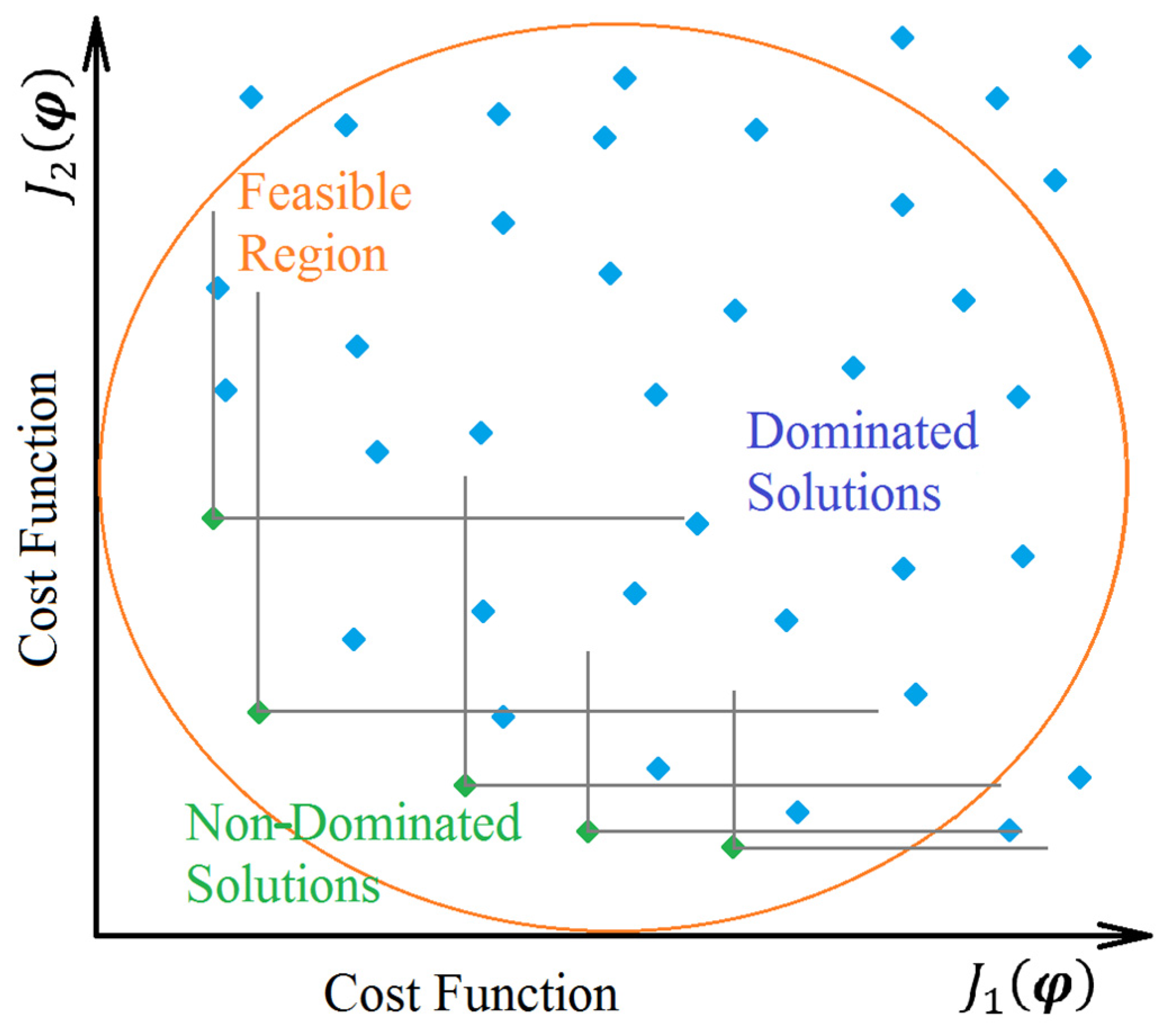
4.1. Multiobjective Problem Statement

The Equation (17) shows a general MOP formulation [32], where the goal is to simultaneously minimize $n$ objectives, $J_i\left(\mathit{\phi }\right)$, $i=\left[1,2,\dots ,n\right]$, of a variable vector $\mathit{\phi } \left(1\times m\right)$ with $l$ inequality constraints and $q$ equality constraints, see Equation (18). In a control problem, the coefficients of the minimization function $\left[x_1,x_2,\dots ,x_m\right]$ represent the gains of the controller.

$$\underset{\mathit{\phi }}{\min }J\left(\mathit{\phi }\right)=\left[J_1\left(\mathit{\phi }\right),J_2\left(\mathit{\phi }\right),\dots ,J_i\left(\mathit{\phi }\right)\right]$$

(17)

where

$$\begin{array}{c}\mathit{\phi }=\left[x_1,x_2,\dots ,x_m\right], \mathrm{subject} \mathrm{to} g_j\left(\mathit{\phi }\right)\le 0, j=\left[1,2,\dots ,l\right],\\ h_k\left(\mathit{\phi }\right)=0, k=\left[1,2,\dots ,q\right].\end{array}$$

(18)

The first step is associated with the definition of a parametric model that will be used to perform computational simulations to calculate the cost functions. In control applications, a transfer function is assumed as a parametric model. The transfer function can be obtained through a system identification procedure [50], or through physical modeling. In Section 2, two models were described and assumed for the ball and beam apparatus while considering the physical modeling approach.

The second step is the cost functions definition. In this case, at least one error criterion, this being related to the performance of the system, and one robustness criterion, which is associated with controllers’ confidence, are assumed. Frequently, the performance criterion is related to the minimization of the error signal, improving the system capability to follow the reference and reject disturbances in the system, as presented in Equations (13) and (14). On the other hand, the robustness criterion considers the behavior of the control signal that is subject to noises and unexpected variations in the working cycles, see Equations (15) and (16).

4.2. Multiobjective Optimization Process

The multiobjective optimization stage is dedicated to obtaining a set of possible solutions for the control problem, which is represented by the parametric model and associated with the minimization of the cost functions. In the case of non-conflicting objectives, a single solution can be considered to be an optimal solution, and the use of additional methods to analyze the set of solutions is not necessary. However, when conflicting objectives are considered, the final result of the optimization process is a set of solutions that are defined as non-dominated solutions, named the Pareto Front [45]. In this case, a ranking criterion can be assumed to define the optimal solution.

The multiobjective optimization techniques are strategies that can be used to approximate the Pareto Front. These techniques are classified into two basic types: the direct methods, and multiobjective evolutionary algorithms [51].

The direct methods are a class of algorithms that are oriented by the iterations of previous results according to the descending information, e.g., gradient information, presenting fast convergence and searching efficiency. Nevertheless, this kind of algorithm has some problems when the gradient is hard to, or cannot be, calculated, frequently getting trapped in local optimal solutions [52]. Some strategies for approximating the Pareto Front through direct methods are the Normal-Boundary Intersection (NBI) [53], the Physical Programming [54], the Normalized Normal Constraint method [55], among others.

In another way, the multiobjective evolutionary algorithms are stochastic optimization techniques, where, at each iteration, the cost functions are evaluated for each individual, obtaining the dominance relations among the solutions. This information is used to select potentially better solutions and produce the next generation [56]. Some metaheuristics that can be used for this purpose are the Nondominated Sorting Genetic Algorithm II (NSGA-II) [57], the Multi-Objective Artificial Bee Colony Algorithm with Regulation Operators (RMOABC) [58], and the Adaptive Multiswarm Comprehensive Learning Particle Swarm Optimization (AMCLPSO) [59], among others.

4.3. Multicriteria Decision Making

The multicriteria decision-making stage is the last step of the multiobjective optimization design procedure, where a method is applied to select a reasonable solution for the problem that is based on the conflicting criteria of the objective functions.

There are two main approaches for applying MCDM techniques, one considering a single method and others assuming multiple multicriteria methods. In the first approach, the decision-maker should have knowledge regarding the MOP to decide which objective function will be emphasized. In the second approach, while considering multiple MCDM methods, the main idea is to adequately visualize the decision scene defining a mathematical model to reflect the decision-maker preferences. In this way, it is possible to reduce the set of solutions, and to then solve the mathematical model while using another MCDM technique, i.e., the set of solutions is successively reduced [49].

Some interesting examples of MCDMs that can be directly applied to select a candidate solution in the Pareto Front are the cooperative solutions of the bargaining games [60]. These can be divided into the Nash solution (Ns), the Kalai–Smorodinsky solution (K-Ss), and the Egalitarian solution (Es). Both cooperative solutions need the specification of a utopian solution and a disagreement point to be founded, and these points consist of the best (even impossible) situation and the combination of the worst value for each cost function for all of the candidate solutions, respectively. The Ns is a solution selected from the set of candidates where the biggest volume (n-dimensional, depending on the number of cost functions) is obtained, starting from the disagreement point until the candidate solution evaluated. The K-Ss is the candidate solution in the point of intersection between a line connecting the points of disagreement and the utopian solution and the Pareto Front, and the Es is obtained through the intersection of a line, which started in the disagreement point and had an angle of 45 degrees, and the Pareto Front.

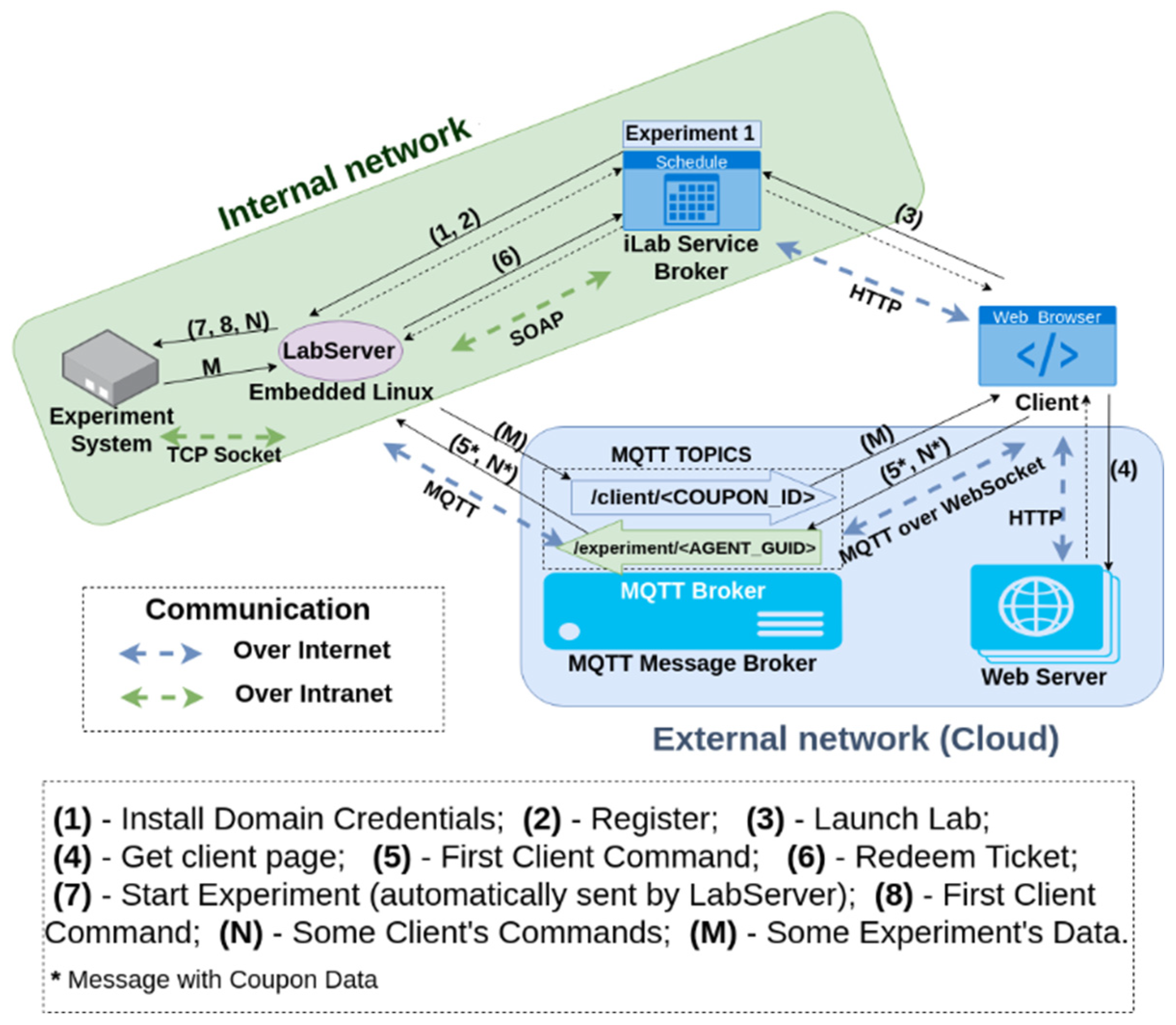
5. Remote Experiment Description

This section describes the remote experiment structure, followed by procedures that have to be performed by the students along an advanced control course.

5.1. Experiment Structure

The control system of the remote ball and beam experiment was hosted on a Raspberry Pi 3 microcomputer, which was connected to the university network. This microcomputer, called a lab server, is intended to receive commands from a user while considering an interface hosted on a cloud server. This cloud server communicates with the lab server through an MQTT protocol-based architecture.

The user must connect to a service broker to access the remote experiment. After authorized access, the date and time scheduling routine can be configured. After that, the user can perform a remote experiment. Once authorized to run the experiment, the user is redirected to the interface webpage of the experiment, where he will perform the actions and collect datasets of his results that will be stored on a storage server for later access if needed. The architecture that is described here is called ISA—iLab Shared Architecture [61].

Additionally, the operating system that is used for both the lab server and the interfaces located on the cloud server consists of Linux distributions. For programming, the control systems of the remote experiment, as well as communication via MQTT, the Python programming language was used. Additionally, for the programming of the controller of the remote experiment, the C language was considered.

Figure 10 illustrates all of the architecture described above, which is composed of the cloud server, the lab server, the communication protocols, and the intermediation of this communication through ISA. This architecture was called ELSA-SP.

First, the user accesses the ISA server through a university-provided internet address by entering login and password data. In the sequence, the user selects the desired date and time to access the experiment. Once the date and time were configured, the user requests the access and the execution of the experiment. ISA will send an access coupon containing data, such as user ID, server ID, and passkey to the lab server. The lab server checks on a new ISA connection whether the coupon is correct and, if it is, ISA provides a ticket to the lab server containing access data and the duration of the experiment. The lab server authorizes the execution of the experiment by informing ISA of the ticket data. ISA, which has ticket data, finally authorizes the user to access and operate the experiment interface.

The main contribution that is expected through experimentation procedures in control engineering courses is to assist in the critical review in studies of advanced control. In this way, the ball and beam system can be used in the comparison between the configuration and analyses of the controller’s parameters. Additionally, the controller’s performance obtained while considering two methods can also be verified. In this case, the first approach usually assumes a classical controller tuning rules, and the second one is based on multiobjective optimization with evolutionary algorithms.

5.2. Experimental Procedures

This section presents the experimental procedures that are associated with the control of the ball and beam system. A sampling time of $100$ ms was considered, and the additional parameters are the ball radius, $R=2.0$ cm, its mass, $m=50$.0 g; the rolling radius was measured as $r=1.65$ cm, and the beam length of $1$ m.

For the remote experimental procedures, we suggest two distinct control structures that are based on PD control action. The first one considers a cascade controller with an integrator as a high-frequency filter. Additionally, the beam angle control was performed, as shown in Figure 11. The second one with the derivative part in the feedback loop, as shown in Figure 12. The second structure with the derivative term in the feedback loop is an interesting approach, as students can analyze and understand how to reduce the noise amplification.

Figure 13 presents the sequence for the experimental approach. The basis of the study is structured in four main stages to be followed: (i) to simulate the models presented in Section 2 of this article, the simplified model (3), and the full model (13); (ii) to use a classical controller tuning rule to define the controllers’ parameters. Some interesting methods for this purpose can be found in [63]; (iii) to study MOOP designed for control engineering problems, as described in Section 4. In the sequence, students must define the cost functions, those that are adopted to minimize the performance measures described in Section 3. In this case, MOEA and MCDM methods are both considered; and, (iv) to perform tests of the controllers tuned through distinct methods for the ball and beam WebLab system, when comparing the simulated solutions with the real system performance.

6. Results and Discussion

This section is dived into two subsections in order to illustrate all of the procedures described in Section 4 associated with multiobjective optimization, and results that were obtained while applying the NSGA-II algorithm. The first one shows how the three steps, those that were addressed in Section 4 for multiobjective optimization, were applied to the ball and beam control problem. In the sequence, the results were presented and discussed, showing promising results in assuming EMO strategies for control tuning.

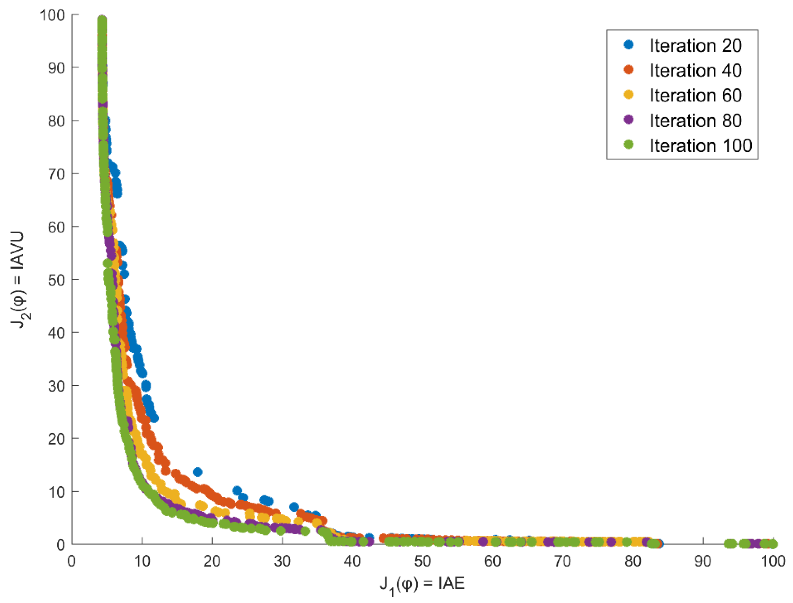
6.1. Multiobjective Optimization Procedures

This subsection describes the procedures applied to the ball and beam process to optimize the controller gains that are based on MOOP.

6.1.1. Problem Definition

The authors assumed the parametric model presented in Figure 11, once it was possible to compare the multiobjective approach to a reference controller already described in [25], in order to define the multiobjective problem associated with the control of the ball and beam apparatus. In this way, a minimization problem was assumed to optimize the controller gains.

$$\underset{\mathit{\phi }\in U}{\min }\left(J_1\left(\mathit{\phi }\right),J_2\left(\mathit{\phi }\right)\right) | J_1\left(\mathit{\phi }\right)={\displaystyle \int }\left|e\left(t\right)\right|dt, \mathrm{and} J_2\left(\mathit{\phi }\right)={\displaystyle \int }\left|\raisebox{1ex}{$du\left(t\right)$}\!\left/ \!\raisebox{-1ex}{$dt$}\right.\right|dt,$$

(19)

where $\mathit{\phi }=\left[K_p,K_d,K_h,K_{p1}\right]$ are the controller’s gain vector, being $K_p$ and $K_d$ the proportional and derivative gains, $K_h$, the high-frequency filter, and $K_{p1}$ the proportional gain that controls the beam angle. All of the gains are restricted to the [0, 50] interval, since the critical gain of the system transfer function tends to infinity. The selected interval was used to simplify the example regarding the search space.

The two cost functions that were presented in Equation (19) were considered. As described in Section 3, the first one represents an error criterion, the Integral of Absolute Error (IAE), and the second one is the control robustness criteria, the Integral of the Absolute Variation of Control Signal (IAVU). While assuming what is presented in Section 4.1, to select both the error and the robustness criteria in the optimization statement improves the confidence in the obtained controller.

6.1.2. Multiobjective Optimization through NSGA-II

Due to interesting results that were presented by the NSGA-II in works that are associated with control applications [64,65,66], this algorithm was assumed in this study. We used the classical multiobjective algorithm NSGA-II, which was described in Algorithm 1 [57], to tune the PD controller applied to the ball and beam apparatus. The PD controller was selected, since the transfer function of the full model described in Equation (13) has two integrators.

Algorithm 1 NSGA-II procedures

1: Initialize the population

2: Evaluate the objective functions for the individuals

3: Rank the individual based on non-dominated sorting

4: Calculate the crowding distance

5: While (Stopping Criteria is not satisfied)

6:      Select the individuals by using a binary tournament for the mating pool

7:      Apply the genetic operators, crossover, and mutation, to the mating pool

8:      Evaluate the objective functions of the offspring population

9:      Combine the offspring population with the current generation

10:    Rank the individual based on non-dominated sorting

11:    Calculate the crowding distance

12:    Select better solutions until complete the size of the population

13: End While

14: Output the non-dominated solutions

A population size of 200 was assumed, and the stopping criterion was based on the number of generations, in this case, being equal to 100. The probability of genetic operations was applied, as proposed in [57], for crossover 90% and, for mutation, the inverse of the number of decision variables, i.e., 25%.

6.1.3. Multicriteria Decision Making Strategy

A set of non-dominated solutions was obtained as the considered optimization strategy is an EMO algorithm. The normalized approximation result was obtained through a linear transformation and is shown in Figure 14 at every 20 iterations, showing the method convergence. The axes of Figure 14 represent the selected cost functions IAE and IAUV.

While considering the set of solutions in the Pareto Front, the Nash solution, as described in Section 4.3, was selected and compared to the reference controller that was provided by the manufacturer [25]. Furthermore, for comparison purposes, the Åström’s robust loop shaping method [29] was applied, and the controller’s gains of the method were obtained while considering a joint sensitivity of 1.4. This value was found on the previously cited reference for a double integer system (see

Table 1. Controller’s gains calculation for the Åström’s robust loop shaping method.

Model	${\mathit{K}}_{\mathit{p}}$	${\mathit{T}}_{\mathit{i}}$	${\mathit{T}}_{\mathit{d}}$
$G_m\left(s\right)=\frac{K_m{e}^{-s{t}_m}}{s^2}$	$\frac{0.0214}{K_m{t}_m^2}$	$17.570t_m$	$14.019t_m$

). We considered, for the time delay, $t_m$, a small approximation of 10 ms, since the method needs a time delay to obtain the controller’s gains. This approximation is one-tenth of the sampling time, and it was just assumed for calculation purpose, as it does not interfere in the system dynamics. For the gain $K_m$, the gravitational force in the city of Curitiba (Brazil) equal to 9.78 m/s² was considered.

Table 2. Controllers’ gains and cost functions values.

	${\mathit{K}}_{\mathit{p}}$	${\mathit{K}}_{\mathit{d}}$	${\mathit{K}}_{\mathit{h}}$	${\mathit{K}}_{\mathit{p}1}$	${\mathit{J}}_1\left(\mathit{\phi }\right)$	${\mathit{J}}_2\left(\mathit{\phi }\right)$
Reference Controller	0.5	0.8	8	8	1931.2	240.4
Optimized Controller	50	11.3588	40.6189	0.1376	1064.7	191.9
	${\mathit{K}}_{\mathit{p}}$	${\mathit{T}}_{\mathit{i}}$	${\mathit{T}}_{\mathit{d}}$		${\mathit{J}}_1\left(\mathit{\phi }\right)$	${\mathit{J}}_2\left(\mathit{\phi }\right)$
Åström Controller	21.8814	0.1757	0.1402	-	1952.0	233.5

presents the controllers’ gain and the cost function values for all of the controllers.

As can be verified in Table 2, the optimized controller performed better than the other controllers for both of the cost functions, with a reduction of 44.87% in the reference tracking error and 20.17% in the control effort when compared to the reference controller. Additionally, a reduction of 45.46% and 17.82% for the error and the control effort were obtained, respectively, when compared to the Åström robust loop shaping method.

In Figure 15, comparisons were performed while considering changes in the desired position of the ball. The output signal of the ball and beam process, which represents the real ball position, was presented while considering the three controllers. Moreover, Figure 16 represents the control signal that is associated with the results that were obtained in Figure 15. In this case, it is important to emphasize the control effort of each strategy. It is also possible to verify that the optimized controller presents an overshoot of 2.6% versus 10.92% for the Åström Controller. Even observing that the Reference Controller did not present an overshoot, its settling time, reduction of the error to a value lesser than 2% from reference, is 2.37 s. When the optimized controller is analyzed in terms of settling time, just 0.83 s was obtained, while the Åström controller provided a 5.30 s for this criterion in positive reference changes.

As previously presented, the use of multiobjective optimization procedures in control engineering can be used to improve the performance of the system. The combination of these procedures can be assumed to be a generalist tool in control tuning problems. A more specific analysis of the ball and beam control case presented in this study showed that the application of the multiobjective optimization procedures that are described in Section 4 increases the possibility of considering distinct control objectives. These objectives could be the classical ones presented in Figure 6 (Section 3) or additional ones that can be defined according to optimization requirements that are associated with the problem.

When remote experimentation is considered, multiobjective optimization can be used to improve students’ knowledge and the quality of the courses that are associated with industrial processes simulations and its challenges, especially when a new and specific process has to be inserted into the academic environment. Moreover, remote experimentation provides a more complex environment in terms of technology integration, as students will not only work with control theory, but with data acquisition, data communication, and virtual instrumentation, technologies that are being assumed in the recent context of industry 4.0.

7. Conclusions

This research started presenting an overview of the essential learning methods that are used in the control engineering learning, as well as the importance that is associated with the approximation of the academic to the industrial area. As the next step, a brief description of the ball and beam process, which represents an example of a complex system that is frequently found in industry, was addressed. The third section presented the PID control theory, showing two variations that can be found in the literature to control the ball and beam system. Additionally, metrics that were commonly used as performance measures related to both the error and the control effort were described. Section 4 presents the multiobjective optimization approach that was related to control engineering problems, while Section 5 showed the experimental structure for the WebLab and experimental procedures assumed in this study. Finally, Section 6 reported how the presented method is effective in comparison with a classical control tuning approach, emphasizing the advantages of applying multiobjective optimization in the educational context that is associated with control engineering.

The use of WebLabs in education is an interesting tool for improving the quality of control engineering courses, since it is possible to improve the diversity of experiments and approximate the challenges of industrial areas to the academic space. The present research proposed a sequential method for the use of WebLabs that is associated with PID tuning problems, where the use of computational intelligence through multiobjective optimization design was applied.

The control of the ball and beam plant, which is a nonlinear and unstable open-loop process, is a common problem that students will find in industry, and the comparison between the classical direct tuning method with the multiobjective optimization strategy provides a better understanding of the advantages of assuming EMO techniques for similar problems that are associated to control systems.

WebLabs can be used to improve the availability of the laboratory structures for experimentation processes while considering a collaboration network. The implementation costs for this solution is around US$3000.00. The ball and beam plant cost is US$2500.00, the lab server, US$60.00, the cloud server, US$200.00/year, and other devices can be estimated at US$240.00. These values are related to the implementation of the structure in a Brazilian university.

For future works, we will expand on the use of intelligent control systems through multiobjective optimization for other processes, while also including the use of fuzzy systems for specialist control, and machine learning methods that can be used in the identification procedures while focusing on the obtention of parametric models, these procedures that are always associated with virtual laboratories. Additionally, a formal analysis focusing on the feedback provided by the students will also be performed. Previous results that are associated with the students’ feedback indicated that this type of methodology is understood as the future of engineering learning, once the industry demand nowadays is directly associated with connected machines, integrated systems, and real-time information analysis.

References

1. Ogata, K. Modern Control Engineering, 5th ed.; Pearson: Upper Saddle River, NJ, USA, 2010; ISBN 9780136156734. [Google Scholar]
2. Hernández-Guzmán, V.M.; Silva-Ortigoza, R. Automatic Control with Experiments; Advanced Textbooks in Control and Signal Processing; Springer International Publishing: Cham, Switzerland, 2019; ISBN 978-3-319-75803-9. [Google Scholar] [CrossRef]
3. Gan, B.; Menkhoff, T.; Smith, R. Enhancing students’ learning process through interactive digital media: New opportunities for collaborative learning. Comput. Hum. Behav. 2015, 51, 652–663. [Google Scholar] [CrossRef]
4. Roberto, J.; Peña, Q.; Oliveira, J.; Leonel, M.; Henrique, L.; Rodrigues, N. Active Methodologies in Education of Electronic Instrumentation Using Virtual Instrumentation Platform Based on Labview and Elvis II. In Proceedings of the 2018 IEEE Global Engineering Education Conference (EDUCON), Islas Canarias, Spain, 17–20 April 2018; pp. 1696–1705. [Google Scholar]
5. Maskeliunas, R.; Damaševičius, R.; Lethin, C.; Paulauskas, A.; Esposito, A.; Catena, M.; Aschettino, V. Serious game iDO: Towards better education in dementia care. Information 2019, 10, 355. [Google Scholar] [CrossRef] [Green Version]
6. Araujo, V.; Mendez, D.; Gonzalez, A. A Novel Approach to Working Memory Training Based on Robotics and AI. Information 2019, 10, 350. [Google Scholar] [CrossRef] [Green Version]
7. Cheng, K.W.E.; Chan, C.L. Remote hardware controlled experiment virtual laboratory for undergraduate teaching in power electronics. Educ. Sci. 2019, 9, 222. [Google Scholar] [CrossRef] [Green Version]
8. Selmer, A.; Kraft, M.; Moros, R.; Colton, C.K. Weblabs in Chemical Engineering Education. Educ. Chem. Eng. 2007, 2, 38–45. [Google Scholar] [CrossRef] [Green Version]
9. Oliveira, O.N., Jr. Research Landscape in Brazil: Challenges and Opportunities. J. Phys. Chem. 2016, 120, 5273–5276. [Google Scholar] [CrossRef] [Green Version]
10. Zheng, P.; Wang, H.; Sang, Z.; Zhong, R.Y.; Liu, Y.; Liu, C.; Mubarok, K. Smart manufacturing systems for Industry 4.0: Conceptual framework, scenarios, and future perspectives. Front. Mech. Eng. 2018, 13, 137–150. [Google Scholar] [CrossRef]
11. Raz, A.K.; Blasch, E.; Cruise, R.; Natarajan, S. Enabling Autonomy in Command and Control Via Game-Theoretic Models and Machine Learning with a Systems Perspective. AIAA Scitech Forum 2019. [Google Scholar] [CrossRef]
12. Carreras Guzman, N.H.; Mezovari, A.G. Design of IoT-based Cyber—Physical Systems: A Driverless Bulldozer Prototype. Information 2019, 10, 343. [Google Scholar] [CrossRef] [Green Version]
13. De Torre, L.; Guinaldo, M.; Heradio, R.; Dormido, S. The Ball and Beam System: A Case Study of Virtual and Remote Lab Enhancement With Moodle. IEEE Trans. Ind. Inform. 2015, 11, 934–945. [Google Scholar] [CrossRef]
14. Hauser, J.; Sastry, S.; Kokotović, P. Nonlinear control via approximate input-output linearization: The ball and beam example. IEEE Trans. Automat. Control 1992, 37, 392–398. [Google Scholar] [CrossRef]
15. Chang, B.C.; Kwtany, H.; Hu, S.-S. An Application of Robust Feedback Linearization to a Ball and Beam Control Problem. In Proceedings of the IEEE International Conference on Control Applications, Trieste, Italy, 4 September 1998; pp. 694–698. [Google Scholar]
16. Lo, J.; Kuo, Y. Decoupled Fuzzy Sliding-Mode Control. IEEE Trans. Fuzzy Syst. 1998, 6, 426–435. [Google Scholar]
17. Ali, T.; Adeel, M.; Malik, S.A.; Amir, M. Stability Control of Ball and Beam System Using Heuristic Computation Based PI-D and PI-PD Controller. Tech. J. Univ. Eng. Technol. 2019, 24, 21–29. [Google Scholar]
18. Ding, M.; Liu, B.; Wang, L. Position control for ball and beam system based on active disturbance rejection control. Syst. Sci. Control Eng. 2019, 7, 97–108. [Google Scholar] [CrossRef] [Green Version]
19. Almutairi, N.B.; Zribi, M. On the sliding mode control of a Ball on a Beam system. Nonlinear Dyn. 2010, 59, 221–238. [Google Scholar] [CrossRef]
20. Keshmiri, M.; Jahromi, A.F.; Mohebbi, A.; Amoozgar, M.H.; Xie, W. Modeling and control of ball and beam system using model based and non-model based control approaches. Int. J. Smart Sens. Intell. Syst. 2012, 5, 14–35. [Google Scholar] [CrossRef] [Green Version]
21. Chang, Y.; Chan, W.; Chang, C.T.-S. Fuzzy Model-Based Adaptive Dynamic Surface Control for Ball and Beam System. IEEE Trans. Ind. Electron. 2013, 60, 2251–2263. [Google Scholar] [CrossRef]
22. Osinski, C.; La, A.; Silveira, R. Control of Ball and Beam System Using Fuzzy PID Controller. In Proceedings of the 2018 13th IEEE International Conference on Industry Applications (INDUSCON), São Paulo, Brazil, 12–14 November 2018; IEEE: New York, NY, USA; pp. 875–880.
23. Storn, R.; Price, K. Differential Evolution—A Simple and Efficient Heuristic for Global Optimization over Continuous Spaces. J. Glob. Optim. 1997, 11, 341–359. [Google Scholar] [CrossRef]
24. Shah, M.; Ali, R.; Malik, F.M. Control of Ball and Beam with LQR Control Scheme using Flatness Based Approach. In Proceedings of the 2018 International Conference on Computing, Electronic and Electrical Engineering (ICE Cube), Quetta, Pakistan, 12–13 November 2018; IEEE: New York, NY, USA; pp. 1–5. [Google Scholar]
25. Tecquipment Academia. Ball and beam apparatus. In CE106: User manual; Tecquipment: Nottingham, UK, 1993; p. 132. [Google Scholar]
26. Khalore, A.G. Relay Approach for tuning of PID controller. Int. J. Comput. Technol. Appl. 2012, 3, 1237–1242. [Google Scholar]
27. Åström, K.J. PID controllers: Theory, Design and Tuning; Instrument society of America: Pittsburgh, PA, USA, 1995. [Google Scholar]
28. Sain, D. PID, I-PD and PD-PI controller design for the ball and beam system: A comparative study. Int. J. Control Theory Appl. 2016, 9, 9–14. [Google Scholar]
29. Åström, K.; Hägglund, T. Advanced PID Control; ISA—Instrumentation Systems and Automation Society: Research Triangle Park, NC, USA, 2006. [Google Scholar]
30. Goldberg, D.E. Genetic Algorithms in Search, Optimization, and Machine Learning, 2nd ed.; Addison-Wesley: Boston, MA, USA, 1989; ISBN 0-201-15767-5. [Google Scholar]
31. Kagami, R.M.; Reynoso-Meza, G.; Santos, E.A.P.; Freire, R.Z. Control of a Refrigeration System Benchmark Problem: An Approach based on COR Metaheuristic Algorithm and TOPSIS Method. IFAC-PapersOnLine 2019, 52, 85–90. [Google Scholar] [CrossRef]
32. Marler, R.T.; Arora, J.S. Survey of multi-objective optimization methods for engineering. Struct. Multidiscip. Optim. 2004, 26, 369–395. [Google Scholar] [CrossRef]
33. Venkata Rao, R. Jaya: A simple and new optimization algorithm for solving constrained and unconstrained optimization problems. Int. J. Ind. Eng. Comput. 2016, 7, 19–34. [Google Scholar] [CrossRef]
34. Tangherloni, A.; Rundo, L.; Nobile, M.S. Proactive Particles in Swarm Optimization: A Settings-Free Algorithm for Real-Parameter Single Objective Optimization Problems. In Proceedings of the 2017 IEEE Congress on Evolutionary Computation (CEC), San Sebastian, Spain, 5–8 June 2017; pp. 1940–1946. [Google Scholar] [CrossRef]
35. Rueda, J.; Erlich, I. Hybrid Population Based MVMO for Solving CEC 2018 Test Bed of Single-Objective Problems. In Proceedings of the 2018 IEEE Congress on Evolutionary Computation (CEC), Rio de Janeiro, Brazil, 8–13 July 2018. [Google Scholar] [CrossRef] [Green Version]
36. Fan, Z.; Fang, Y.; Li, W.; Yuan, Y.; Wang, Z.; Bian, X. LSHADE44 with an Improved ϵ Constraint-Handling Method for Solving Constrained Single-Objective Optimization Problems. In Proceedings of the 2018 IEEE Congress on Evolutionary Computation, Rio de Janeiro, Brazil, 8–13 July 2018; IEEE: New York, NY, USA; pp. 1–8. [Google Scholar] [CrossRef]
37. Zhao, Z.; Wang, X.; Wu, C.; Lei, L. Hunting optimization: An new framework for single objective optimization problems. IEEE Access 2019, 7, 31305–31320. [Google Scholar] [CrossRef]
38. Azlan, N.A.; Yahya, N.M. Modified Adaptive Bats Sonar Algorithm with Doppler Effect Mechanism for Solving Single Objective Unconstrained Optimization Problems. In Proceedings of the 2019 IEEE 15th International Colloquium on Signal Processing & Its Applications (CSPA), Penang, Malaysia, 8–9 March 2019; pp. 27–30. [Google Scholar] [CrossRef]
39. Feliot, P.; Bect, J.; Vazquez, E. A Bayesian approach to constrained single- and multi-objective optimization. J. Glob. Optim. 2017, 67, 97–133. [Google Scholar] [CrossRef] [Green Version]
40. Han, H.; Lu, W.; Zhang, L.; Qiao, J. Adaptive gradient multiobjective particle swarm optimization. IEEE Trans. Cybern. 2017, 48, 3067–3079. [Google Scholar] [CrossRef]
41. Azwan, A.; Razak, A.; Jusof, M.F.M.; Nasir, A.N.K.; Ahmad, M.A. A multiobjective simulated Kalman filter optimization algorithm. In Proceedings of the 2018 IEEE International Conference on Applied System Invention (ICASI), Chiba, Japan, 13–17 April 2018; pp. 23–26. [Google Scholar] [CrossRef]
42. Zhang, M.; Wang, H.; Cui, Z.; Chen, J. Hybrid multi-objective cuckoo search with dynamical local search. Memetic Comput. 2018, 10, 199–208. [Google Scholar] [CrossRef]
43. Antunes, C.H.; Alves, M.J.; Clímaco, J. Multiobjective Linear and Integer Programming; Springer International Publishing: Cham, Switzerland, 2016; ISBN 978-3-319-28744-7. [Google Scholar] [CrossRef]
44. Reynoso-Meza, G.; Garcia-Nieto, S.; Sanchis, J.; Blasco, F.X. Controller tuning by means of multi-objective optimization algorithms: A global tuning framework. IEEE Trans. Control Syst. Technol. 2013, 21, 445–458. [Google Scholar] [CrossRef] [Green Version]
45. Miettinen, K. Nonlinear Multiobjective Optimization; International Series in Operations Research & Management Science; Springer: Boston, MA, USA, 1998; Volume 12, ISBN 978-1-4613-7544-9. [Google Scholar] [CrossRef]
46. Ojha, M.; Singh, K.P.; Chakraborty, P.; Verma, S. A review of multi-objective optimisation and decision making using evolutionary algorithms. Int. J. Bio-Inspired Comput. 2019, 14, 69–84. [Google Scholar] [CrossRef]
47. Coello, C.C.A.; Lamont, G.B.; Van Veldhuizen, D.A. Evolutionary Algorithms for Solving Multi-Objective Problems; Genetic and Evolutionary Computation Series; Springer: Boston, MA, USA, 2007; Volume 139, ISBN 978-0-387-33254-3. [Google Scholar] [CrossRef]
48. Reynoso-Meza, G.; Blasco Ferragud, X.; Sanchis Saez, J.; Herrero Durá, J.M. Controller Tuning with Evolutionary Multiobjective Optimization; Intelligent Systems, Control and Automation: Science and Engineering; Springer International Publishing: Cham, Switzerland, 2017; Volume 85, ISBN 978-3-319-41299-3. [Google Scholar] [CrossRef]
49. Yano, H. Interactive Multi-Objective Decision Making under Uncertainty; CRC Press: Boca Raton, FL, USA, 2017; ISBN 9781498763547. [Google Scholar]
50. Ljung, L. System Identification: Theory for the User; PTR Prentice-Hall: Hemel Hempstead, UK, 1987; ISBN 0138816409. [Google Scholar]
51. Reynoso-Meza, G. Controller Tuning by Means of Evolutionary Multiobjective Optimization: A Holistic Multiobjective Optimization Design Procedure; Universitat Politècnica de València: Valencia, Spain, 2014. [Google Scholar] [CrossRef]
52. Cui, Y.; Geng, Z.; Zhu, Q.; Han, Y. Review: Multi-objective optimization methods and application in energy saving. Energy 2017, 125, 681–704. [Google Scholar] [CrossRef]
53. Das, I.; Dennis, J. Normal-Boundary Intersection: An Alternate Method for Generating Pareto Optimal Points in Multicriteria Optimization. Nasa Contract. Rep. 1996. [Google Scholar] [CrossRef] [Green Version]
54. Messac, A.; Mattson, C.A. Generating well-distributed sets of pareto points for engineering design using physical programming. Optim. Eng. 2002, 3, 431–450. [Google Scholar] [CrossRef]
55. Messac, A.; Ismail-Yahaya, A.; Mattson, C.A. The normalized normal constraint method for generating the Pareto frontier. Struct. Multidiscip. Optim. 2003, 25, 86–98. [Google Scholar] [CrossRef]
56. Gunantara, N. A review of multi-objective optimization: Methods and its applications. Cogent Eng. 2018, 5. [Google Scholar] [CrossRef]
57. Deb, K.; Pratap, A.; Agarwal, S.; Meyarivan, T. A fast and elitist multiobjective genetic algorithm: NSGA-II. IEEE Trans. Evol. Comput. 2002, 6, 182–197. [Google Scholar] [CrossRef] [Green Version]
58. Huo, J.; Liu, L. An improved multi-objective artificial bee colony optimization algorithm with regulation operators. Information 2017, 8, 18. [Google Scholar] [CrossRef] [Green Version]
59. Yu, X.; Estevez, C. Adaptive multiswarm comprehensive learning particle swarm optimization. Information 2018, 9, 173. [Google Scholar] [CrossRef] [Green Version]
60. Thomson, W. Cooperative Models of Bargaining. In Handbook of Game Theory with Economic Applications; Aumann, R.J., Hart, S., Eds.; Elsevier: Amsterdam, The Netherlands, 1994; Volume 2, pp. 1237–1284. [Google Scholar]
61. Harward, V.J.; del Alamo, J.A.; Lerman, S.R.; Bailey, P.H.; Carpenter, J.; DeLong, K.; Felknor, C.; Hardison, J.; Harrison, B.; Jabbour, I.; et al. The iLab Shared Architecture: A Web Services Infrastructure to Build Communities of Internet Accessible Laboratories. Proc. IEEE 2008, 96, 931–950. [Google Scholar] [CrossRef]
62. Uhlmann, T.S.; Lima, H.D.; Luppi, A.L.; Mendes, L.A. ELSA-SP-Through-The-Cloud Subscribe-Publish Scheme for Interactive Remote Experimentation under iLab Shared Architecture and Its Application to an Educational PID Control Plant. In Proceedings of the 2019 5th Experiment at International Conference, exp.at 2019, Funchal, Portugal, 12–14 June 2019; pp. 58–62. [Google Scholar] [CrossRef]
63. O’Dwyer, A. Handbook of PI and PID Controller Tuning Rules, 3rd ed.; Imperial College Press: London, UK, 2009; ISBN 9781848162426. [Google Scholar]
64. Esmaeili, M.; Shayeghi, H.; Aryanpour, H.; Nooshyar, M. Design of new controller for load frequency control of isolated microgrid considering system uncertainties. Int. J. Power Energy Convers. 2018, 9, 285. [Google Scholar] [CrossRef]
65. Yegireddy, N.K.; Panda, S.; Papinaidu, T.; Yadav, K.P.K. Multi-objective non dominated sorting genetic algorithm-II optimized PID controller for automatic voltage regulator systems. J. Intell. Fuzzy Syst. 2018, 35, 4971–4975. [Google Scholar] [CrossRef]
66. Deng, T.; Lin, C.; Luo, J.; Chen, B. NSGA-II multi-objectives optimization algorithm for energy management control of hybrid electric vehicle. Proc. Inst. Mech. Eng. Part D J. Automob. Eng. 2019, 233, 1023–1034. [Google Scholar] [CrossRef]
Figure 1. The ball and beam process used as a case study in this research [25].
Information 11 00132 g001
Figure 2. The movement of the sphere is affected by gravity when the beam is not on the horizontal position.
Information 11 00132 g002
Figure 3. Angular velocity definition of the ball.
Information 11 00132 g003
Figure 4. Ball velocity diagram.
Information 11 00132 g004
Figure 5. Graphic representation of the radius.
Information 11 00132 g005
Figure 6. Performance coefficients.
Information 11 00132 g006
Figure 7. Block diagrams of Proportional-Integral-Derivative (PID) control variations: (a) Proportional Integral-Derivative (PI-D); and, (b) Integral-Proportional Derivative (I-PD).
Information 11 00132 g007
Figure 8. Multiobjective optimization procedures for control systems (adapted from [44]).
Information 11 00132 g008
Figure 9. Representation of both non-dominated and dominated solutions in the cost functions domain.
Information 11 00132 g009
Figure 10. ELSA-SP structure (adapted from [62]).
Information 11 00132 g010
Figure 11. PD design for the ball and beam apparatus.
Information 11 00132 g011
Figure 12. Alternative PD design for the ball and beam apparatus.
Information 11 00132 g012
Figure 13. Experimental procedures to be developed by the students.
Information 11 00132 g013
Figure 14. The obtained set of non-dominated solutions with normalized cost functions.
Information 11 00132 g014
Figure 15. System response to reference changes for the different controllers.
Information 11 00132 g015
Figure 16. The control signal from different controllers for the reference changes.
Information 11 00132 g016