Article

Noninvasive Blood Pressure Classification Based on Photoplethysmography Using K-Nearest Neighbors Algorithm: A Feasibility Study

by
Hendrana Tjahjadi
* and
Kalamullah Ramli
*
Author to whom correspondence should be addressed.
Information 2020, 11(2), 93; https://doi.org/10.3390/info11020093
Submission received: 16 December 2019 / Revised: 23 January 2020 / Accepted: 28 January 2020 / Published: 9 February 2020
(This article belongs to the Section Artificial Intelligence)

Abstract

:
Blood pressure (BP) is an important parameter for the early detection of heart disease because it is associated with symptoms of hypertension or hypotension. A single photoplethysmography (PPG) method for the classification of BP can automatically analyze BP symptoms. Users can immediately know the condition of their BP to ensure early detection. In recent years, deep learning methods have presented outstanding performance in classification applications. However, there are two main problems in deep learning classification methods: classification accuracy and time consumption during training. We attempt to address these limitations and propose a method for the classification of BP using the K-nearest neighbors (KNN) algorithm based on PPG. We collected data for 121 subjects from the PPG–BP figshare database. We divided the subjects into three classification levels, namely normotension, prehypertension, and hypertension, according to the BP levels of the Joint National Committee report. The F1 scores of these three classification trials were 100%, 100%, and 90.80%, respectively. Hence, it is validated that the proposed method can achieve improved classification accuracy without additional manual pre-processing of PPG. Our proposed method achieves higher accuracy than convolutional neural networks (deep learning), bagged tree, logistic regression, and AdaBoost tree.

Graphical Abstract

1. Introduction

Blood pressure (BP) is a vital parameter for the primary detection of cardiovascular diseases. Hypertension is one of the most significant risk factors for cardiovascular diseases [1]. The outcome of a BP measurement consists of three parameters, namely the diastolic blood pressure (DBP), systolic blood pressure (SBP), and mean arterial pressure (MAP), in millimeters of mercury (mmHg) [2,3,4]. There are two categories of methods for determining BP: invasive and noninvasive methods. While invasive methods can measure BP precisely and continuously, they are not very suitable to apply and trigger infections in patients [5]. The noninvasive methods that are presently implemented using a cuff cause discomfort, particularly for injured people, overweight people, and infants [6].
Many innovations have been developed to measure BP without a cuff continuously and the most promising one is photoplethysmography (PPG) [7,8,9,10]. The generation of PPG signals needs some optoelectronic components: a light-emitting diode (LED) and a photodetector. Figure 1 illustrates an example of a PPG waveform containing direct current (DC) and alternating current (AC) components. The DC component of the PPG waveform relates to the reflected optical signal from the tissue and depends on the configuration of the tissue and the average blood volume of both arterial and venous blood. The DC component fluctuates slowly with respiration, while the AC component shows blood volume changes, which occur between the systolic and diastolic phases of the cardiac cycle. The essential frequency of the AC component depends on the heart rate and is covered onto the DC component [11]. An LED is a light source that can be used to illuminate blood vessels so minor perfusion changes can be supervised on the photodetectors [12]. Perfusion is measured as the degree at which blood is distributed to tissue [13].
ECG together with PPG signals are the most common combination for assessing BP in cuff-less continuous monitoring systems, because they are essential for calculating the pulse transit time (PTT). Teng, X.F et al. [14] examined the relationships between arterial BP and certain features of the PPG. Kim, J.Y et al. [15] measured PTT using PPG and electrocardiogram (ECG) signals and biometric parameters such as weight, height, body mass index (BMI) length of arm and circumference of arm. Y.S. Yan et al. [16] examined a new feature, normalized harmonic area (NHA), which is extracted from PPG signals in the period domain by using the discrete period transform (DPT). McCombie et al. [17] proposed a technique for calibrating the measured pulse wave velocity (PWV) to arterial blood pressure using hydrostatic pressure variation. Studies have shown that the correlation between BP and PTT is significant, but depends on many parameters which can vary among different patients. Therefore the calibration is needed when used in every new patient. The PTT-based BP calculation may not be sufficiently precise because the regulation of BP in the human body is a complex and multivariate physiological process.
To overcome this issue, several calibration-free methods were proposed for accurate and reliable estimation of BP. There is a relation, not always linear, between blood pressure and pulse duration, obtained from PPG signal. They use a combination of machine learning and signal processing algorithms or artificial neural network with multilayer feed-forward back propagation algorithm. Kurylyak et al. [18] proposed a non-invasive continuous BP estimation approach based on artificial neural networks (ANNs). Rundo et al. [19] proposed a physiological ECG/PPG “combo” pipeline using an innovative bio-inspired nonlinear system based on a reaction–diffusion mathematical model, implemented by means of the convolution neural network (CNN) methodology, to filter PPG signal by assigning a recognition score to the wave forms in the time series. However, all these methodologies present the disadvantage that they are based on PTT calculation, which requires ECG/PPG hardware sensors, software, data extraction (PTT and PWV), etc., making them complicated when applied.
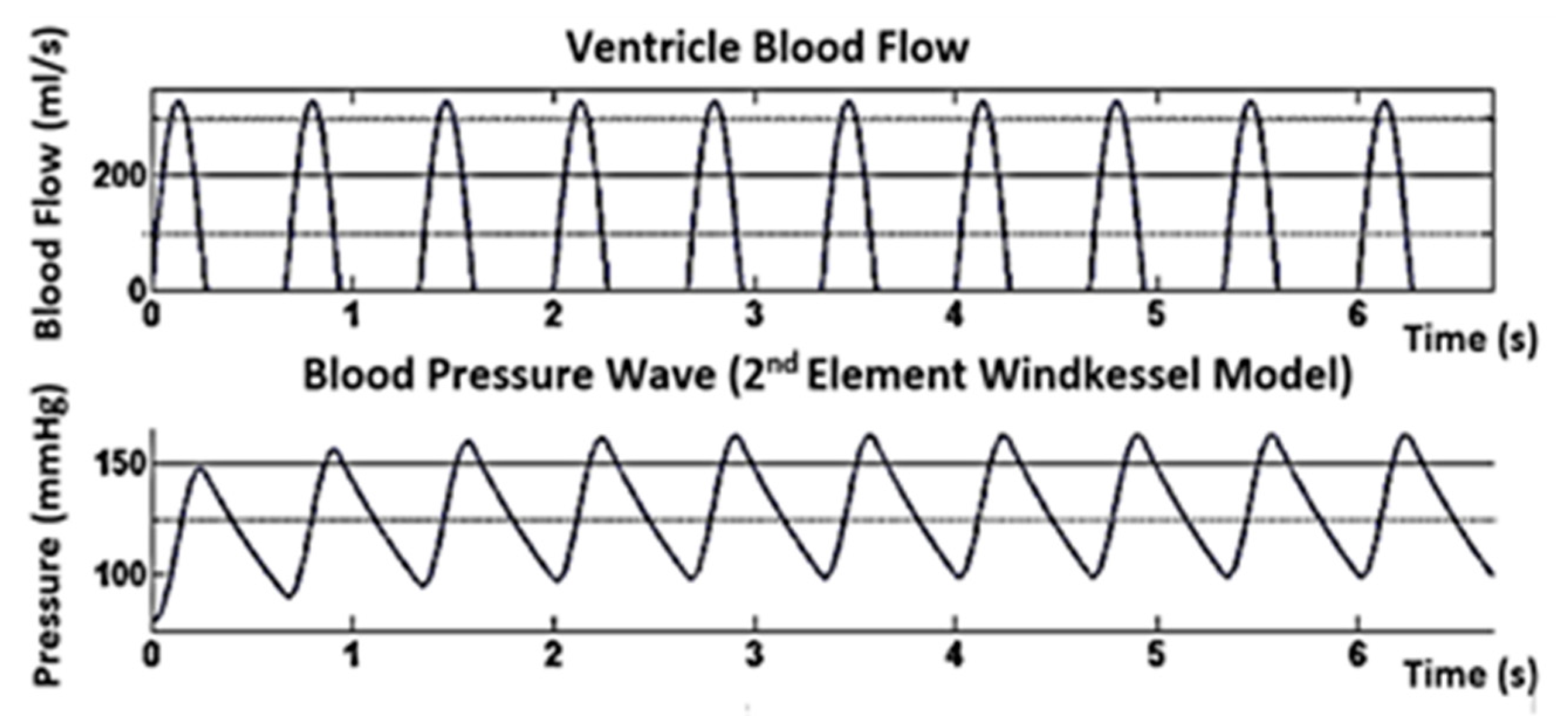
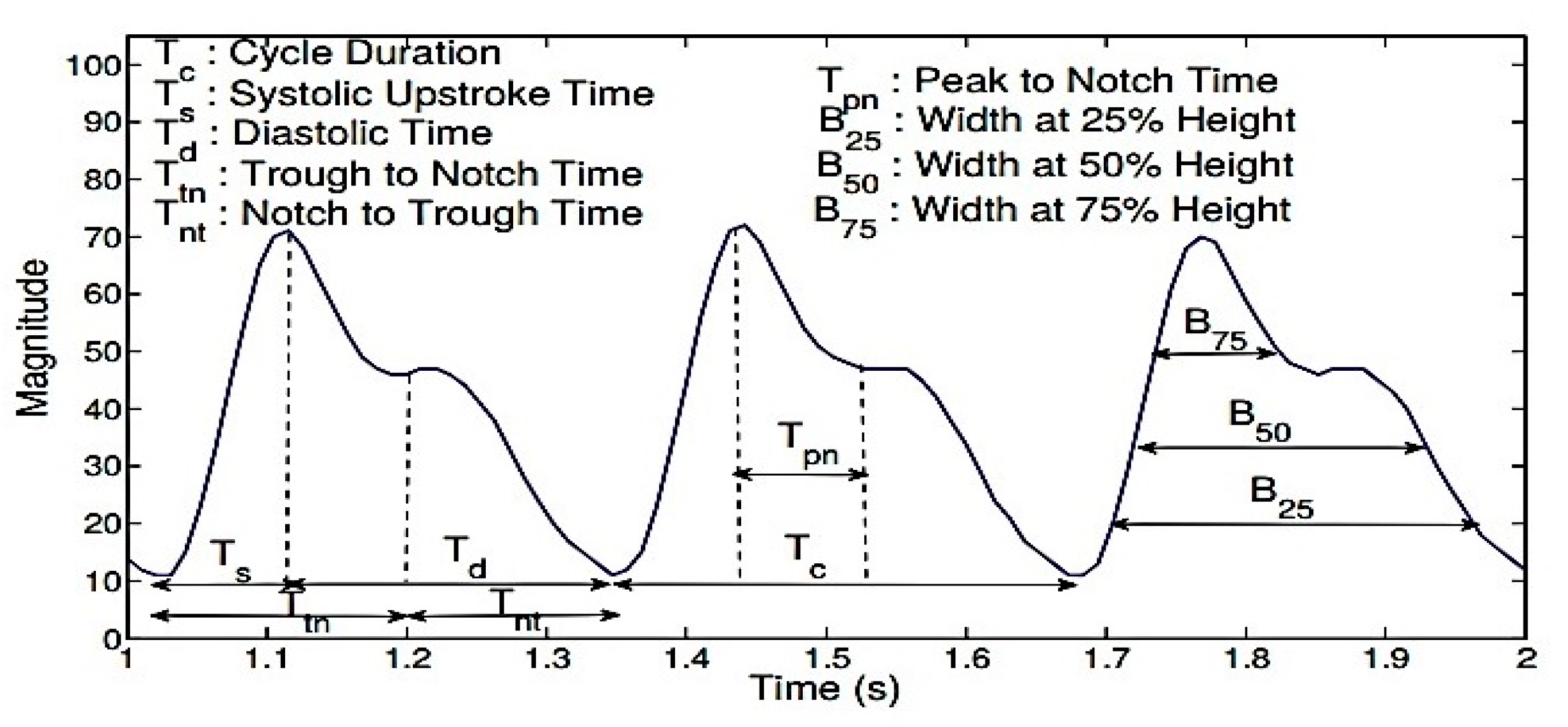
The features of PPG are also recognized to carry important information that can be used as physiological parameters. Indeed, our previous work has presented statistical evidence that the features of PPG can be used to assess BP [20]. A single PPG-based BP estimation study was conducted to make users more comfortable [10,11,12,13]. Presently, there are two methods to reach BP estimation using single PPG. The first method is a parametric model that challenges to extract certain parameters such as the systolic, heart rate, and diastolic periods from every PPG waveform. BP estimation can be achieved using these parameters [13]. Numerous examples of parametric methods include regression of long- and short-term features, the pulse transport theory-based model, linear regression [13], and the Windkessel model. The second element of the Windkessel method estimates the entire peripheral resistance and regulates the value of the body’s arterial capacitance through the PPG waveform, as shown in Figure 2. Parametric models can achieve good expectation results for an individual, but the accuracy declines over time. Besides, these methods need an initial calibration and frequent recalibrations for every person. The second method involves nonparametric models, which try to extract specific features in the frequency domain or time domain, as shown in Figure 3 [11].
There are numerous potential sources of mistakes in BP estimation methods based on PPG:
  • The PPG waveform is easily affected by motion artifacts, leading to errors in the measurement [21,22,23,24,25]. Most motion artifacts associate with the sensor motion relative to the skin [26]. The dimensions of the finger have a significant contribution. Therefore, the pressure applied to the fingers is hard to control. This situation greatly influences PPG waveforms and reduces the accuracy of BP estimates [18].
  • The system must be calibrated to regulate varying PPG waveform characteristics [27,28,29]. The quality of the PPG waveform is easily corrupted by poor blood circulation, and PPG waveform characteristics vary with fluctuations in peripheral vascular resistance, blood vessel wall elasticity, and blood viscosity [19]. PPG waveforms are easily affected; consequently, the connection between peripheral pulses and BP may not be optimal [21]. Therefore, the system needs frequent recalibrations for every person [22]. There is not sufficient evidence to provide a calibration-free BP estimation with PPG signals only.
  • BP estimation methods based on PPG do not actually measure pressure. Instead, they use waveform feature analysis and theoretical models to calculate the hemodynamics and associate them to BP [23].
  • Most importantly, the actual volume measured by PPG is the total amount of hemoglobin, which is considered to be proportional to the volume of blood. This hypothesis may fail in patients with anemia or edema [24].
  • Cold temperature triggered by diseases can also reduce the correlation between peripheral pulsation and blood pressure [25]. High blood viscosity reduces blood flow and significantly impacts the PPG waveform [27]. Hypertension may also be attended by arrhythmia diabetes or pregnancy, which may introduce unknown parameters to the method and reduce the fitting accuracy [28].
However, most previous studies have attended to the estimation of BP value. With these methods, medical supervision is still needed [29,30]. Blood pressure classification methods can automatically analyze BP symptoms. Users can instantaneously know their BP condition to provide an early warning system for potential patients. Visvanathan et al. [31] used a support vector machine to classify BP values. The classification process was performed using the radial basis function kernel. BP values were collected from the Multiparameter Intelligent Monitoring in Intensive Care Database. They divided the BP value range into bins of hypotension, desired, prehypertension, Stage 1 hypertension, Stage 2 hypertension, and hypertensive. Their proposed method with frequency domain features was first tested with the University of Queensland’s vital signs dataset, which covers a wide range of BP values, recorded from 32 surgical cases ranging in duration from 13 min to 5 h over four weeks at the Royal Adelaide Hospital. They proposed an effective feature extraction approach using the concept of maximal information coefficient. Liang. Y et al. [26] used four distinctive classifiers: logistic regression, AdaBoost tree, bagged tree, and K-nearest neighbors (KNN) for blood pressure classification. These studies usied PAT and PPG features extracted from ECG and PPG signals. Three BP classifications were defined as normotension (NT), prehypertension (PHT), and hypertension (HT). The KNN classifier presented the best performance compared with the other models. Additionally, the feature set of the PAT feature and 10 PPG features achieved higher accuracy than the other models. Liang. Y et al. [26] discussed the early screening of hypertension while using the morphological features of photoplethysmography (PPG). Numerous morphological features of PPG and its derivative waves were defined and extracted. Six types of feature selection methods were chosen to screen and evaluate these PPG morphological features. The data processing and modeling estimations were carried out using MATLAB software. The F1 scores for the normotension versus prehypertension, normotension and prehypertension versus hypertension, and normotension versus hypertension trials were 83.34%, 94.84%, and 88.49%, respectively. Based on the ranked features, multiple classifications were conducted using the top 10 features. In these studies, KNN (K = 10) showed better performance in classifying the different BP categories.
In recent years, deep learning methods have presented their outstanding performance in pattern recognition applications [32]. Liang. Y et al. examined in depth learning methods for classifying BP based on PPG signals using the continuous wavelet transformation (CWT) and convolutional neural networks (CNNs) [33]. To classify BP based on a PPG signal, three classification experiments were conducted: normotension (NT) versus prehypertension (PHT), normotension (NT) versus hypertension (HT), and NT + PHT versus HT. They used 80% of the dataset for training and the remaining 20% for testing. Data records were obtained from the MIMIC physiological database with a 125 Hz sampling rate containing atrial BP and PPG signals. The F1 scores for the NT vs. PHT, NT vs. HT, and (NT + PHT) vs. HT trials were 80.52%, 92.55%, and 82.95%, respectively. The specific disadvantages of their studies are summarized as follows:
  • They require higher processing power and properties. The computation difficulty was high and, consequently, considered during the training stage.
  • They need extra training time. The training stage was too long. The training set contained 2323 images and the testing set contained 581 images. For these thousands of images, the training time of each trial lasted more than 350 min.
  • They need training with large-scale data.
However, there are two main problems in deep learning classification methods: the classification accuracy and time consumption during training. We attempt to address these limitations and propose a method for the classification of BP using the K-nearest neighbors algorithm based on PPG. The proposed method is suitable for real-time blood pressure classification. K-nearest neighbors is one of the simplest supervised machine learning algorithms and is mostly used for classification. Our main contributions are as follows:
  • We focus on a BP classification based on the Joint National Committee (JNC 7). Therefore, in this study, three BP classification levels were established: normotension (NT), prehypertension (PHT), and hypertension (HT). With our proposed method, users can immediately know the condition of their blood pressure. Accordingly, this method can expedite the treatment process and reduce the risk of mortality.
  • With our proposed method, a special process is not needed to warranty the PPG signal’s quality and excludes the need for a calibration process.
  • Our proposed method uses machine learning instead of deep learning to achieve a faster training time. The common problem of deep learning is that the training stage is too long.
This paper is organized as follows. Section 2 describes the methodology. The experimental results are given in Section 3. Section 4 discusses the results. The conclusion is presented in Section 5.

2. Materials and Methods

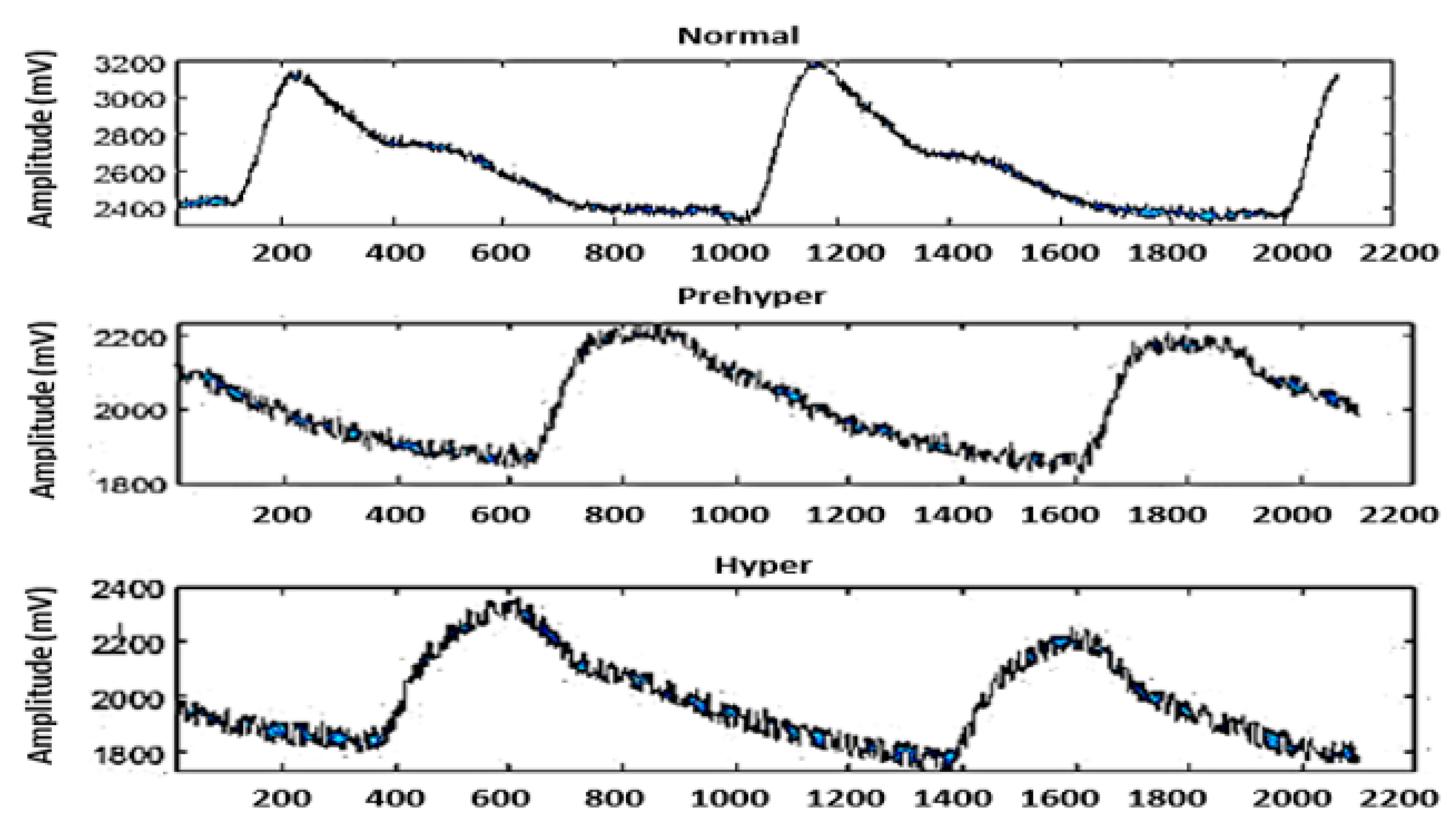
The original PPG signals were shared from a PPG–BP figshare database [34]. We divided the data into signal and label groups. The signals were a cell array consisting of a collection of PPG signals. The labels were an array of categories that contained the ground-truth labels from the signal. Then, we split the signal group into a training set to train the classifier and a testing set to test the accuracy of the classifier. The input one-dimensional PPG time domain was divided into BP levels for adults into three main categories, namely normotension, prehypertension, and hypertension, according to the BP levels of the Joint National Committee report. Waveforms of the PPG signals are shown in Figure 4. To prevent bias, datasets were added by duplicating the signal data from each classification level until each group had the same number of datasets (290 normal subjects, 290 subjects, and 290 hypertension signals). In this study, a confusion matrix was used to visualize classifier performance for a dataset where the true values are known. To comprehensively evaluate the testing models, various evaluation indices were used, including accuracy (Ac), recall (Re), specificity (Sp), precision (Pr), sensitivity (Se), and the F1 scores.

2.1. Data Acquisition

The dataset was collected from 219 adult subjects aged 21–86 years. Males accounted for 48% of the participants. We collected 870 recorded data from the PPG–BP Figshare database [34]. A dataset collection program was written to obtain information about individual basic physiology, which also collected PPG waveform signals and detected the arterial BP at the same time. The dataset includes PPG and BP information from subjects who were diagnosed with normotension, prehypertension, and hypertension. The records include an identification number, sex, age, and disease. The total duration of the experiment was approximately 15 min. The data collected from the PPG signals and BP took approximately 3 min. Each data segment consisted of 2100 sampling points, which corresponded to 2.1 s of data. The waveform was sampled at a frequency of 1 kHz during the signal acquisition, with a 12-bit analog-to-digital conversion precision. The waveform signal quality evaluation method adopted the skewness signal quality index (SSQI) (more details about the dataset can be found in [34]).
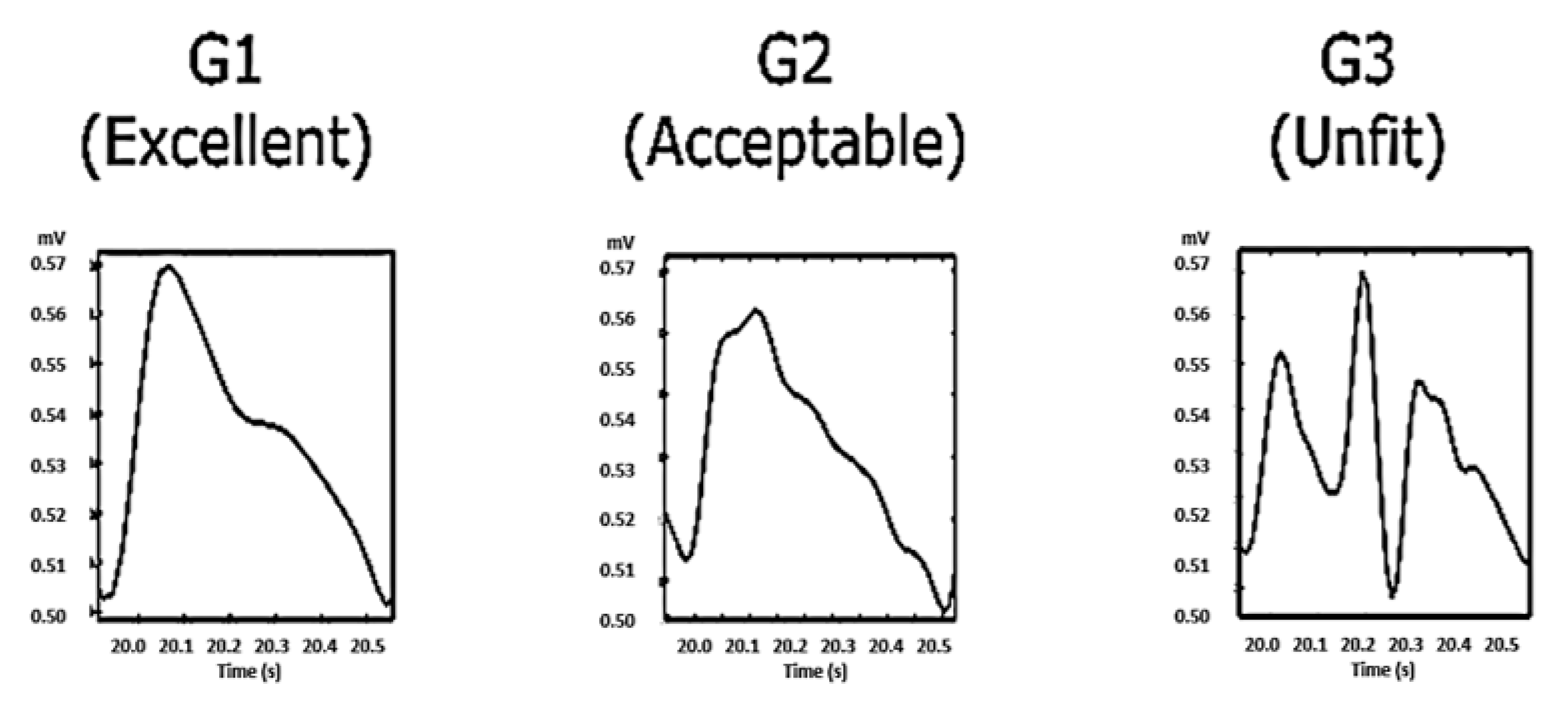
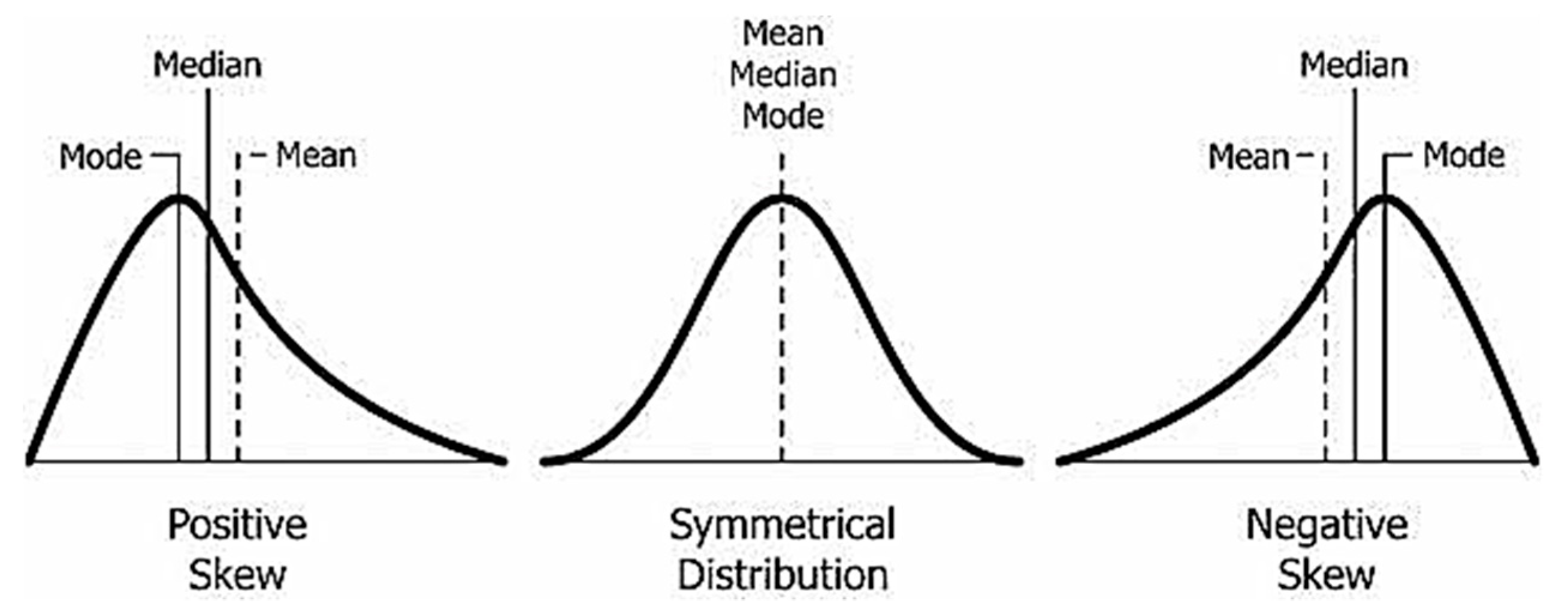
Skewness characterizes the degree of asymmetry of a given distribution around its mean. If the distribution of the data is symmetric, then the skewness will be close to 0. Positive skewness indicates a distribution with an asymmetric tail extending toward more positive values. Negative skewness indicates a distribution with an asymmetric tail extending toward more negative values, as shown in Figure 5. Each segment of the PPG signal was evaluated by classification thresholds as an excellent, acceptable, or unfit PPG waveform to determine whether it should be saved, as detailed in Figure 6. [35]. This step was developed to reduce the PPG segments with high noise and motion artifacts. Skewness is used to measure the probability distributions of symmetric signals. Mathematicians discuss skewness in terms of the third moment around the mean. The specific definition is as follows [35]:
S SQI   =   i = 1 N ( A i A ¯ ) 3 ( N 1 ) σ 3
where SSQI is the skewness signal quality index, N is the number of variables in the distribution, σ is the standard distribution, Aᵢ is a random variable, and A ¯ is the mean of the distribution.

2.2. K-Nearest Neighbors Algorithm

KNN is one of the simplest supervised machine learning algorithms and is mostly used for classification [35]. It classifies a data point based on how its neighbors are classified. It is basically based on the idea that objects near each other will have similar characteristics. The nearest neighbor rule is the simplest form of KNN when K = 1. In this method, each sample must be classified the same as the neighbor sample. Therefore, if the classification of the sample is not identified, it can be predicted by considering the classification of the nearest neighbor sample. Therefore, unidentified samples can be classified based on this classification of closest neighbors [36].

2.2.1. Distance Metric

As mentioned above, KNN makes predictions based on the result of the K-neighbors closest to that point. Hence, to create predictions with KNN, we need to describe a metric for calculating the distance between the request point and cases from the example sample. The KNN makes predictions based on results from the neighbor K closest to that point. Therefore, to make predictions with KNN, we need to determine the metric to calculate the distance between the request point and the case reference point from the sample. One of the most common distance metrics for measuring this distance is known as the Euclidean distance [36]. The Euclidean distance can be described by:
i = 1 k ( x i y i ) 2
where x and y are the query point and a case from the examples sample, respectively. Notably, the Euclidean distance is only valid for continuous variables such as PPG signals.

2.2.2. K-Nearest Neighbor Predictions

After selecting the value of K, we can make predictions based on KNN examples. For regression, the KNN prediction is the average of the K-nearest neighbors’ outcome [36].
y =   1 K   i = 1 k y i
where yi is the ith case of the examples sample and y is the prediction of the query point. In contrast to regression, in a classification problem, KNN predictions are based on a voting scheme where the winner is used to label the query. Another method is to use large K values at random with more attention to the case closest to the query point. This is achieved by using what is called distance weighting.

2.2.3. Distance Weighting

Since KNN predictions are based on the intuitive assumption that objects close in distance are potentially similar, it makes good sense to discriminate between K-nearest neighbors when making predictions. That is, let the closest points among the K-nearest neighbors have more say in affecting the outcome of the query point. This can be achieved by introducing a set of weights W, one for each nearest neighbor, defined by the relative closeness of each neighbor concerning the query point [36].
W ( x , p i ) =   e x p ( D ( x , p i ) ) i = 1 k e x p ( D ( x , p i ) )
where D(x, pi) is the distance between the query point x and the ith case pi of the example sample.
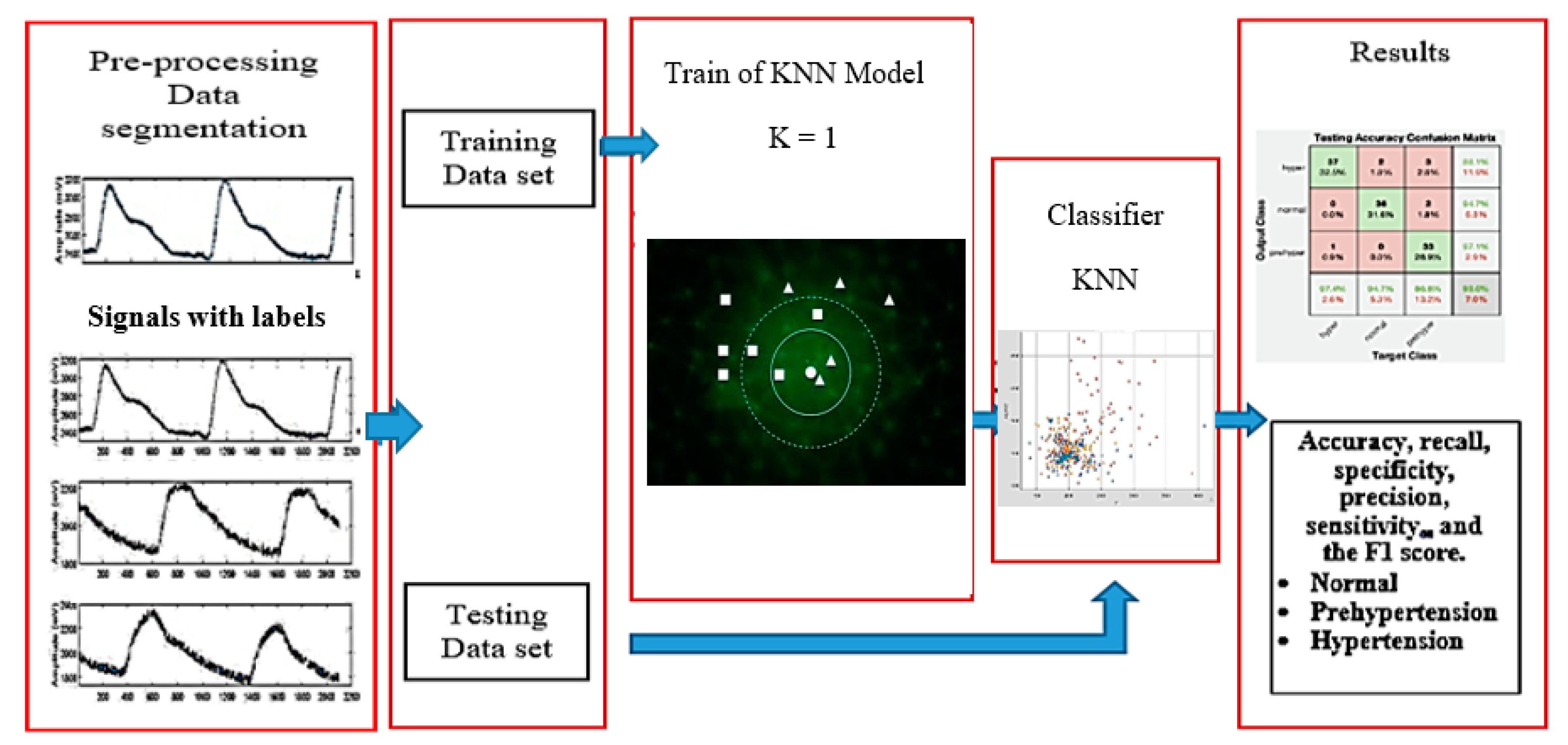
The proposed method consists of training and classification phases. In the training phase, a particular training dataset is extracted and used to train the system using the K-nearest neighbor classifier. In the classification phase, the given test signal is segmented, and then the signal features mentioned above are extracted for classification. These features are questioned to the nearest k-neighbor to be given an unknown signal label. The block diagram of the proposed method is given in Figure 7.

3. Results

We experimented with MATLAB (R2019a version) to classify BP based on PPG signals. In this study, the dataset was divided into a training set and a testing set. We collected data from the PPG–BP figshare database [34] and are available as a MATLAB file extension in Supplementary Materials. The analysis of the PPG features was conducted. Each PPG signal was extracted into 2100 sample points. Feature extraction was carried out point by point so physiological data contained in PPG signals can be explored optimally. It also makes the number of sample points used the largest and most detailed compared to previous studies.
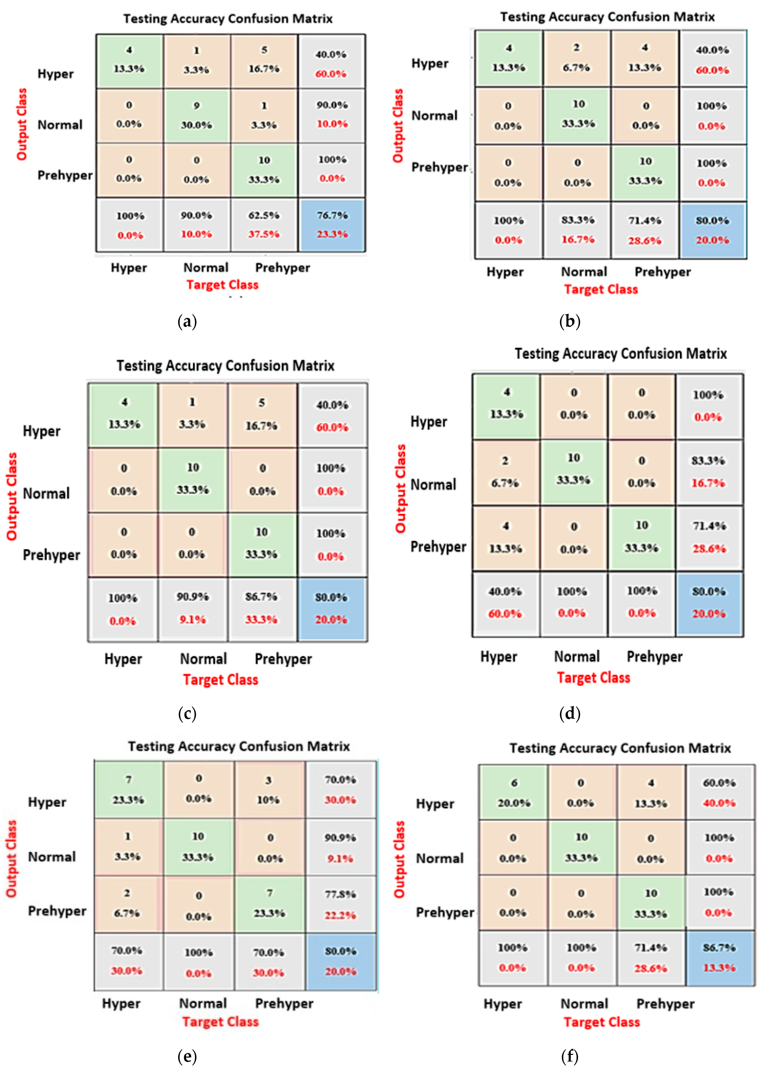
In this study, before deciding which model to use, a comparative analysis was conducted with other models (linier discriminant, decision tree, discriminant analysis, support vector machine, K-nearest neighbor, bagged trees, and deep learning RNN (long short-term memory)) for the same dataset. The dataset was divided into a training set (870 subjects) and a testing set (30 subjects). We compared the testing performance based on accuracy value. The results indicate that KNN algorithm achieved better testing performance than the other classification methods, as shown in Table 1. In this study, a confusion matrix was used to visualize classifier performance for a dataset where the true values are known. The axis labels are the class labels hyper (HT), normal (NT), and prehypertension (PHT). The output class represents the label assigned to the signal by the network.
The target class represents the ground-truth label of the signal. The green cells represent true positive (TP) or true negative (TN) signals. The confusion matrix from the testing process of each model is shown in Figure 8. Based on the results of tests between models, KNN achieved the best results; therefore, this study used KNN as a classifier.
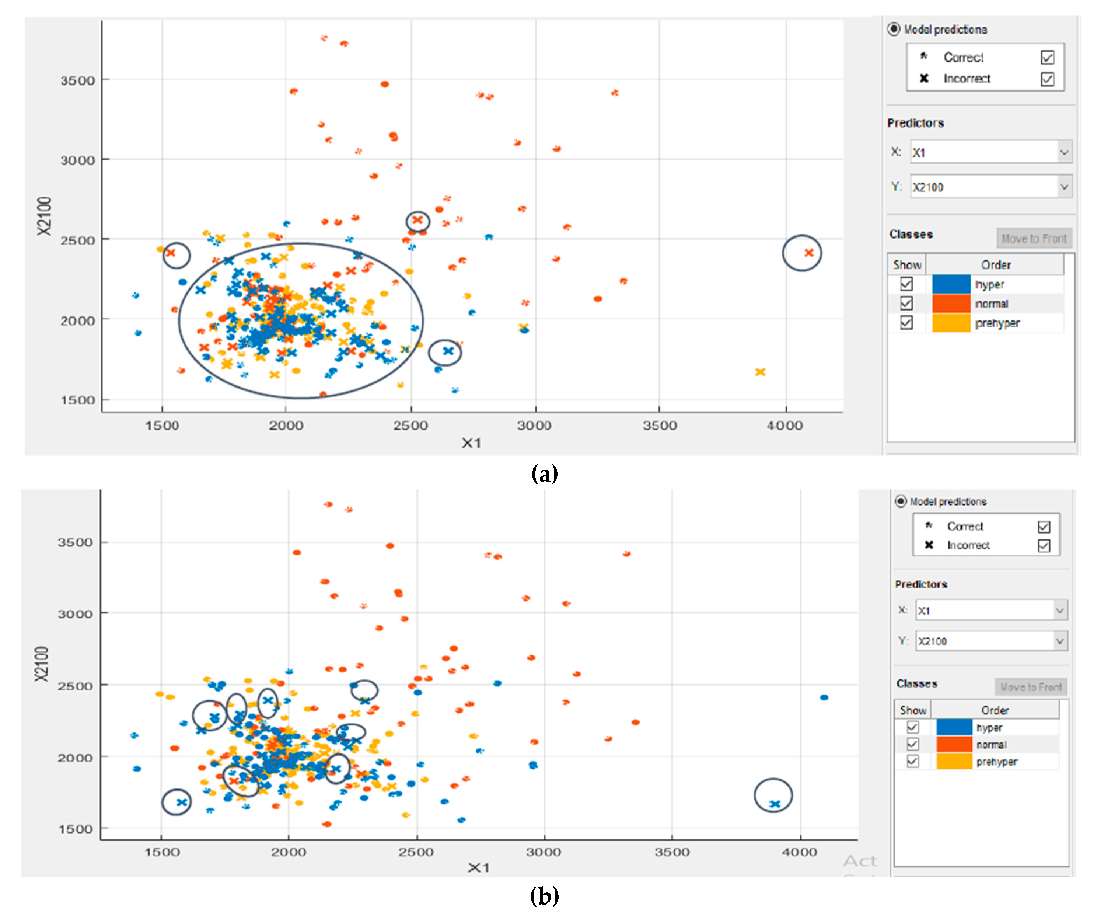
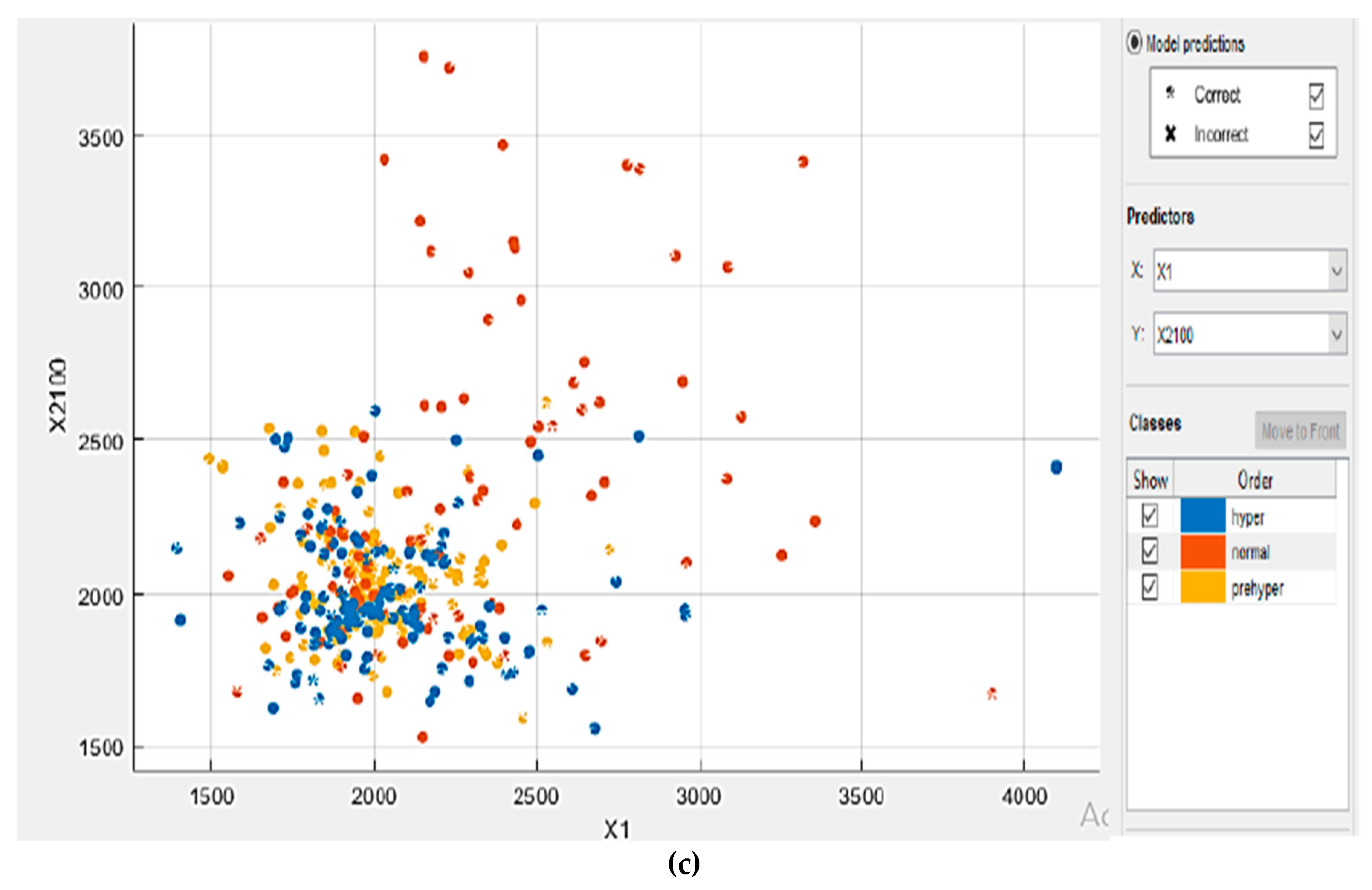
In this proposed KNN model, there are two main parameters: the number of neighbors (K) and the accuracy value that needs to be analyzed. To evaluate these parameters, series of contrast experiments with different training parameter sets were conducted. We tested the contrast experiments with a different number of neighbors to obtain the best accuracy value. When keeping the values of the distance metric (Euclidean), distance weight (equal), and standardized data (true) unchanged, the detailed parameter set is shown in Table 2. The results indicate that KNN algorithm with K value = 1 achieved better training accuracy than the other number of K. The scanter plot can help for investigate features to include or exclude. We can visualize training data and misclassified points on the scatter plot. The scatter plots of a training set with different numbers of neighbors are shown in Figure 9.
To comprehensively evaluate the testing models, various evaluation indices were used: TP, FP, TN, FN, Ac, Re, Sp, Pr, Se, and the F1 score. The confusion matrix used for evaluating the classification performance is as follows [37]:
A c = ( T p + T n T p + F p + T n + F n ) 100 %
R e = ( T p T p + F n ) 100 %
S p = ( T n F p + T n ) 100 %
S e = ( T p T p + F n ) 100 %
P r = ( T p F p + T p ) 100 %
F 1 =   (   2 ( R e   X   P r ) ( R e +   P r )   ) 100 %
where Ac is the accuracy, Re is the recall, Sp is the specificity, Se is the sensitivity, Pr is the precision, and F1 is the F1 score.
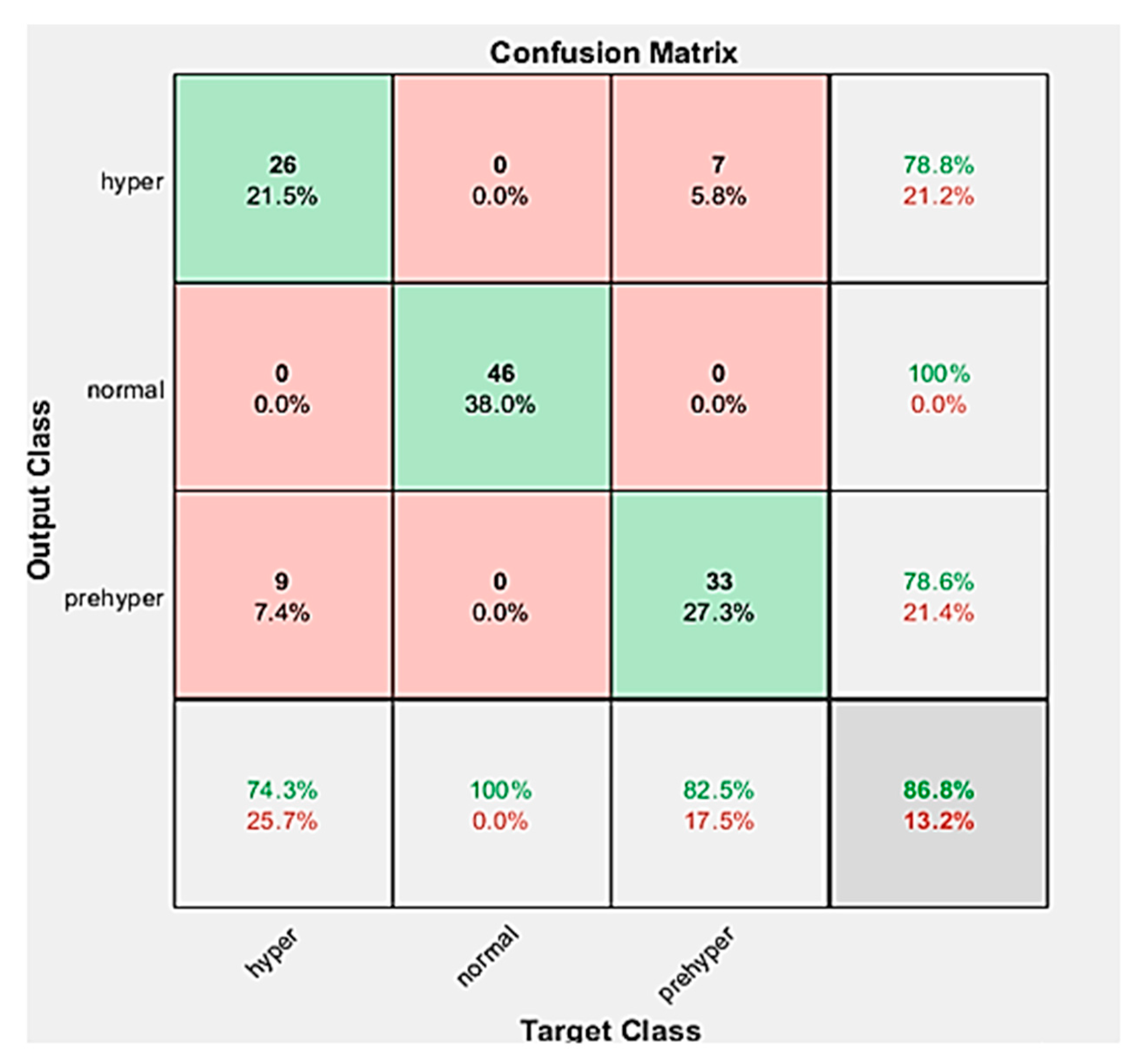
The dataset was divided into a training set (779 subjects) and a testing set (121 subjects). The confusion matrix from the testing process of the KNN algorithm is shown in Figure 10. The confusion matrix of the testing process shows that 74.30% of the ground-truth hyper signals are correctly classified as hyper (HT), 100% of the ground-truth normal signals are correctly classified as normal (NT), and 82.50% of the ground-truth prehyper signals are correctly classified as prehyper (PHT). The above six formulas were computed by the true positive (TP), false positive (FP), true negative (TN), and false negative (FN) quantities. Table 3 shows the classification performance of our proposed method (KNN algorithm). The F1 scores of these three classification trials were 100%, 100%, and 90.80%, respectively.
We performed a comparative study between our method and the results of previous studies [31,33]. To compare BP classifications based on a PPG signal, three classification experiments were carried out: NT (46 subjects) versus PHT (41 subjects), NT (46 subjects) versus HT (34 subjects), and HT (34 subjects) versus PHT + NT (7 subjects). Table 4 presents a performance comparison with earlier studies.

4. Discussion

Our proposed method uses KNN (machine learning) instead of deep learning to achieve faster training times. KNN does not use training data to perform any generalization. In KNN, there is no explicit training phase, or it is very minimal. This also means that the training phase is fast. Lack of generalization means that KNN keeps all the training data. To be more exact, all the training data are needed during the testing phase. We chose KNN as a classifier over other classifiers in the machine learning group because KNN does not require assumptions about data. This situation is suitable for application to nonlinear data such as PPG signals. KNN stores the training dataset and learns from it only at the time of making real-time predictions. This makes the KNN algorithm much faster than other machine learning methods that require training, for example support vector machine (SVM) and linear regression. Since the KNN algorithm requires no training before making predictions, new data can be added seamlessly, which will not impact the accuracy of the algorithm. A disadvantage associated with KNN is that we need to do feature scaling (standardization and normalization) before applying the KNN algorithm to any dataset. Each PPG signal has been extracted into 2100 features. Feature extraction was carried out point-by-point so the physiological data contained in PPG signals can be explored optimally. It also makes the number of features used the largest and most detailed compared to previous studies.
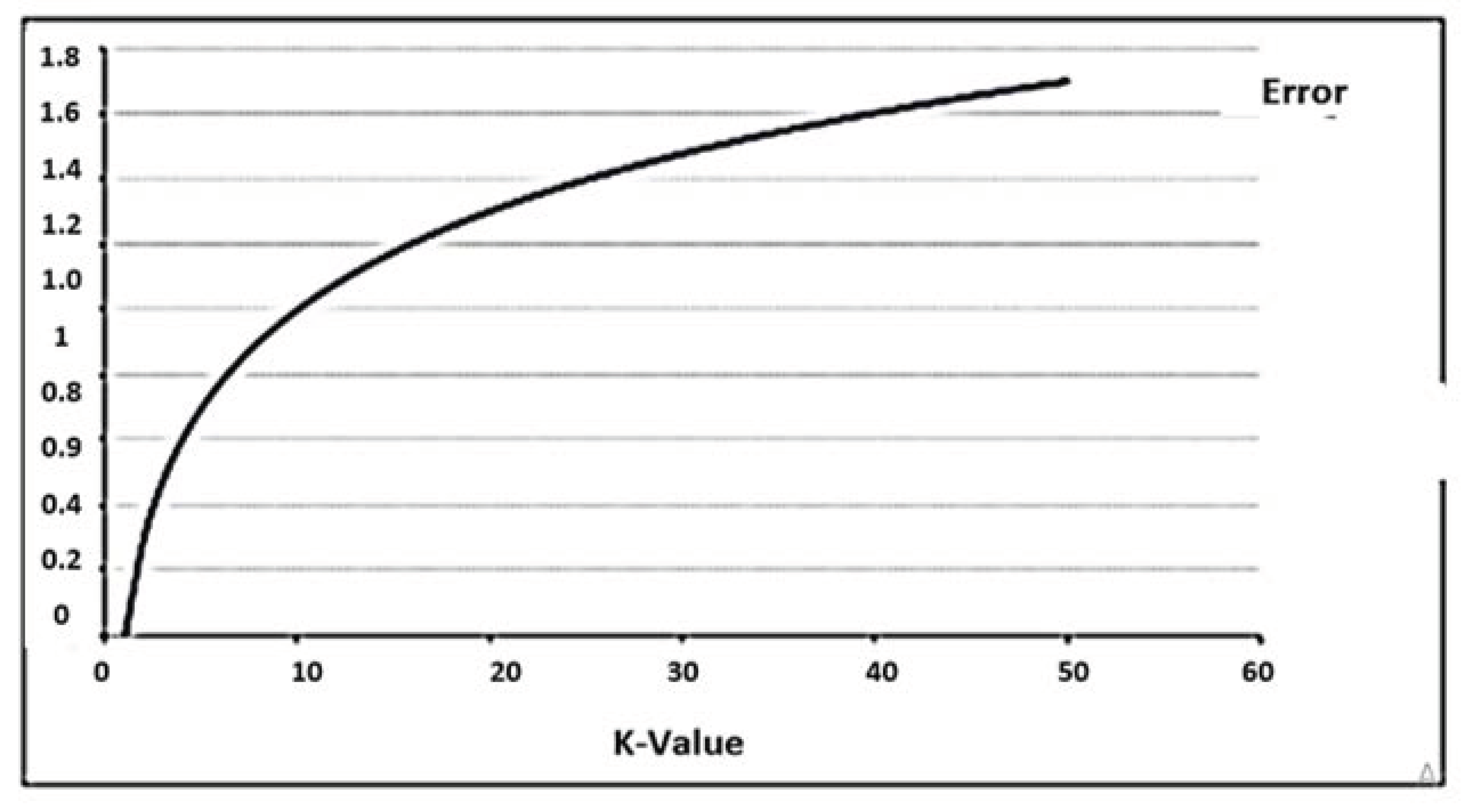
The training error rate and the validation error rate are two parameters we needed to access with different K values. In this study, we made comparisons with several K values, and it was found that K = 1 had the lowest error rate with the highest accuracy value. In Figure 11, the error rate at K = 1 is always zero for the training sample. This is because the closest point to any training data point is itself. Hence, the prediction is always accurate with K = 1.
We performed a comparative study between our method and the results of previous studies [26,33]. The first study by Liang. Y et al. [26] used the PTT-middle to represent the pulse arrival time (PAT) feature, as shown in Figure 12. PAT has some limitations as it cannot classify these three categories of blood pressure levels. Additionally, the combined feature set of the PAT feature and 10 PPG features achieves higher accuracy than other models. The study employed four distinctive classifiers: a bagged tree, K-nearest neighbors (KNN), logistic regression, and an AdaBoost tree. The KNN classifier presented the best performance compared with the other models in the first study by Liang. Y et al. [26], as shown in Table 4. The F1 scores of these three classification trials (NT (46 subjects) vs. PHT (41 subjects), NT (46 subjects) vs. HT (34 subjects), and NT + PHT (87 subjects) vs. HT (34 subjects)) were 83.34%, 94.84%, and 88.49%, respectively. Table 4 shows that the F1 scores of our proposed KNN method were higher than KNN with Liang. Y et al.’s [26] method. The accurate identification of feature points is very important, especially based on the PPG morphology method, and the PPG sampling frequency is the key. In our study, the PPG signal was collected as 1000 Hz sample frequency, whereas the sampling frequency of Liang. Y et al. [26] method is only 125 Hz in the MIMIC database, which could lead to the identification error of each characteristic point. The number of features in the extraction feature greatly affects the level of accuracy of the qualifications. Our study used 2100 PPG features points, whereas Liang. Y et al. [26] used only 10 PPG features. Our method is simpler because it only uses one input signal, i.e. PPG, while Liang. Y et al. [26] used two input signals, namely ECG and PPG, as shown in Table 5.
In the second study of Liang. Y et al. [33], using a continuous wavelet transform (scalogram) and CNNs deep learning for BP classification, the training, unfortunately, took a very long time. They used a training set containing 2323 images, which took about 350 min for training. While our proposed method using a training set of 779 images required a training time of only about 74.116 s. In this case, because the training set was large, the training process could take several minutes. When a network uses data with a large range of values and a large average, the learning process and convergence of the network can be slow [38]. They employed a continuous wavelet transform (Scalogram) and CNNs. The F1 scores of these three classification trials (NT (46 subjects) vs. PHT (41 subjects), NT (46 subjects) vs. HT (34 subjects), and NT + PHT (87 subjects) vs. HT (41 subjects)) were 80.52%, 92.55%, and 82.95%, respectively. Table 4 shows that the F1 scores of our proposed method (KNN) were higher than those of the CNN classifier and regression methods, such as the bagged tree, logistic regression, and AdaBoost tree methods. This result indicates that our proposed method achieved higher accuracy than the CNNs, propagation, and regression methods.

5. Conclusions

Our proposed method has promising potential and exclusively uses raw PPG signals to replace the PPG morphology feature extraction process for BP classification. Users can immediately know the condition of their BP to ensure early detection using our proposed method. This method can expedite the treatment process and reduce the risk of mortality. It is validated that the proposed method classifier using KNN can achieve improved classification accuracy without additional manual pre-processing of the PPG signals. Our proposed method does not require a high-quality PPG signal and does not require the extraction of PPG morphological features; therefore, the method can be easily applied in many situations. In general, normotension has the highest accuracy with a value of 100%. It achieved the best F1 score with a value of 100% among the classification levels. Three classification trials were set: NT vs. PHT, NT vs. HT, and NT + PHT vs. HT. The F1 scores of these three classification trials were 100%, 100%, and 90.80%, respectively. A comparison of current and previous approaches to the classification of BP was accomplished. Our proposed method achieved higher accuracy than convolutional neural networks (deep learning), bagged tree, logistic regression, and AdaBoost tree. In addition, increased sample sizes could be used to further improve the performance of BP classification based on PPG signals.

Supplementary Materials

The following are available online at https://www.mdpi.com/2078-2489/11/2/93/s1. DOI:10. 21227/crpd-4b52.

Author Contributions

H.T. and K.R. conceived, designed, and performed the experiments; methodology, H.T.; software, H.T; review and supervision, K.R.; and all authors contributed to writing the paper. All authors have read and agreed to the published version of the manuscript.

Funding

This research was funded by PDD Grant of Ristekdikti, grant number: NKB-1843/UN2.R3.1/HKP.05.00/2019.

Conflicts of Interest

The authors declare no conflict of interest.

References

  1. Al-Zaben, A.; Fora, M.; Obaidat, A. Detection of Premature Ventricular Beats from Arterial Blood Pressure Signal. In Proceedings of the 2018 IEEE 4th Middle East. Conference on Biomedical Engineering (MECBME), Tunis, Tunisia, 28–30 March 2018; pp. 17–19. [Google Scholar]
  2. Nabeel, P.M.; Karthik, S.; Joseph, J.; Sivaprakasam, M. Arterial blood pressure estimation from local pulse wave velocity using dual-element photoplethysmograph probe. IEEE Trans. Instrum. Meas. 2018, 67, 1399–1408. [Google Scholar] [CrossRef]
  3. Stojanova, A.; Koceski, S.; Koceska, N. Continuous Blood Pressure Monitoring as a Basis for Ambient Assisted Living (AAL) – Review of Methodologies and Devices. J. Med. Syst. 2019, 43, 2. [Google Scholar] [CrossRef] [PubMed]
  4. Shin, H.; Min, S.D. Feasibility study for the non-invasive blood pressure estimation based on ppg morphology: Normotensive subject study. Biomed. Eng. Online 2017, 16, 1–14. [Google Scholar] [CrossRef] [PubMed] [Green Version]
  5. Radha, M.; De Groot, K.; Rajani, N.; Wong, C.C.; Kobold, N.; Vos, V.; Fonseca, P.; Mastellos, N.; Wark, P.A.; Velthoven, N.; et al. Estimating blood pressure trends and the nocturnal dip from photoplethysmograph. Physiol. Meas. 2019, 2, 025006. [Google Scholar] [CrossRef] [Green Version]
  6. Savkar, A.; Khatate, P.; Patil, C.Y. Study on Techniques Involved in Tourniqueteless Blood Pressure Measurement Using PPG. In Proceedings of the in 2018 Second International Conference on Intelligent Computing and Control Systems (ICICCS), Madurai, India, 14–15 June 2019; pp. 170–172. [Google Scholar]
  7. Lin, W.H.; Wang, H.; Samuel, O.W.; Liu, G.; Huang, Z.; Li, G. New Photoplethysmogram Indicators for Improving Cuffless and Continuous Blood Pressure Estimation Accuracy. Physiol. Meas. 2010, 39, 025005. [Google Scholar] [CrossRef]
  8. Tamura, T.; Maeda, Y. Photoplethysmogram. In Seamless Healthcare Monitoring; Springer International Publishing: Cham, Switzerland, 2017. [Google Scholar]
  9. Allen, J. Photoplethysmography and its application in clinical physiological measurement. Physiol. Meas. 2007, 28, R1. [Google Scholar] [CrossRef] [Green Version]
  10. MacKenzie, L.E.; Harvey, A.R. Oximetry using multispectral imaging: Theory and application. J. Optics 2018, 20, 063501. [Google Scholar] [CrossRef] [Green Version]
  11. Datta, S.; Banerjee, R.; Choudhury, A.D.; Sinha, A.; Pal, A. Blood pressure estimation from photoplethysmogram using latent parameters. In Proceedings of the 2016 IEEE International Conference on Communications (ICC), Kuala, Lumpur, 23–27 May 2016. [Google Scholar]
  12. Tjahjadi, H.; Ramli, K. Variance analysis of photoplethysmography for blood pressure measurement. In Proceedings of the 2017 4th International Conference on Electrical Engineering, Computer Science and Informatics (EECSI 2017), Yogyakarta, Indonesia, 19–21 September 2017. [Google Scholar]
  13. Wang, G.; Atef, M.; Lian, Y. Towards a continuous non-invasive cuffless blood pressure monitoring system using PPG: Systems and circuits review. IEEE Circuits Syst. Mag. 2018, 18, 6–26. [Google Scholar] [CrossRef]
  14. Teng, X.F.; Zhang, Y.T. Continuous and noninvasive estimation of arterial blood pressure using a photoplethysmographic approach. In Proceedings of the 25th Annual International Conference of the IEEE Engineering in Medicine and Biology Society, Cancun, Mexico, 17–21 September 2003. [Google Scholar]
  15. Kim, J.Y.; Cho, B.H.; Im, S.M.; Jeon, M.J.; Kim, I.Y.; Kim, S.I. Comparative study on artificial neural network with multiple regressions for continuous estimation of blood pressure. In Proceedings of the 2005 IEEE Engineering in Medicine and Biology 27th Annual Conference, Shanghai, China, 31 August–3 September 2005. [Google Scholar]
  16. Yan, Y.S.; Zhang, Y.T. Noninvasive Estimation of Blood Pressure Using Photoplethysmographic Signals in the Period Domain. In Proceedings of the 2005 IEEE Engineering in Medicine and Biology 27th Annual Conference, Shanghai, China, 31 August–3 September 2005. [Google Scholar]
  17. McCombie, D.B.; Reisner, A.T.; Asada, H.H. Adaptive blood pressure estimation from wearable PPG sensors using peripheral artery pulse wave velocity measurements and multi-channel blind identification of local arterial dynamics. In Proceedings of the 2006 International Conference of the IEEE Engineering in Medicine and Biology Society, New York, NY, USA, 30 August–3 September 2006. [Google Scholar]
  18. Kurylyak, Y.; Lamonaca, F.; Grimaldi, D. A Neural Network-based Method for Continuous Blood Pressure Estimation from a PPG Signal. In Proceedings of the 2013 IEEE International Instrumentation and Measurement Technology Conference (I2MTC), Minneapolis, MN, USA, 6–9 May 2013. [Google Scholar]
  19. Rundo, F.; Ortis, A.; Battiato, S.; Conoci, S. Advanced Bio-Inspired System for Noninvasive Cuff-Less Blood Pressure Estimation from Physiological Signal Analysis. Computation 2018, 6, 46. [Google Scholar] [CrossRef] [Green Version]
  20. Tjahjadi, H.; Ramli, K. Review of photoplethysmography based non-invasive continuous blood pressure methods. In Proceedings of the QiR 2017—2017 15th International Conference on Quality in Research (QiR): International Symposium on Electrical and Computer Engineering, Bali, Indonesia, 24–27 July 2017. [Google Scholar]
  21. Choudhury, A.D.; Banerjee, R.; Sinha, A.; Kundu, S. Estimating blood pressure using Windkessel model on photoplethysmogram. In Proceedings of the 2014 36th Annual International Conference of the IEEE Engineering in Medicine and Biology Society, Chicago, IL, USA, 26–30 August 2014. [Google Scholar]
  22. Blomqvist, K.H.; Kärkkäinen, L. Differential photoplethysmogram sensor with an optical notch filter shows potential for reducing motion artifact signals. Biomed. Phys. Eng. Express Inst. Phys. Eng. Med. 2018, 4, 1–25. [Google Scholar] [CrossRef]
  23. Couceiro, R.; Carvalho, P.; Paiva, R.P.; Henriques, J.; Muehlsteff, J. Detection of motion artifact patterns in photoplethysmographic signals based on time and period domain analysis. Physiol. Meas. 2014, 35, 2369–2388. [Google Scholar] [CrossRef] [PubMed]
  24. Lim, P.K.; Ng, S.C.; Lovell, N.H.; Yu, Y.P.; Tan, M.P.; McCombie, D.; Lim, E.; Redmond, S.J. Adaptive template matching of photoplethysmogram pulses to detect motion artefact. Physiol. Meas. 2018, 39, 105005. [Google Scholar] [CrossRef] [PubMed]
  25. Tamura, T. Current progress of photoplethysmography and SPO2 for health monitoring. Biomed. Eng. Lett. 2019, 9, 21–36. [Google Scholar] [CrossRef] [PubMed]
  26. Liang, Y.; Chen, Z.; Ward, R.; Elgendi, M. Hypertension assessment via ECG and PPG signals: An evaluation using MIMIC database. Diagnostics 2018, 8, 65. [Google Scholar] [CrossRef] [Green Version]
  27. Hassani, A.; Foruzan, A.H. Improved PPG-based estimation of the blood pressure using latent space features. Signal. Image Video Process. 2019. [Google Scholar] [CrossRef]
  28. Chiang, P.Y.; Chao, P.C.P.; Yang, C.Y.; Tarng, D.C. Theoretical developments and clinical experiments of measuring blood flow volume (BFV) at arteriovenous fistula (AVF) using a photoplethysmography (PPG) sensor. Microsyst. Technol. 2018, 24, 4587–4603. [Google Scholar] [CrossRef]
  29. Sanuki, H.; Fukui, R.; Inajima, T.; Shin’ichi Warisawa. Cuff-less Calibration-free Blood Pressure Estimation under Ambulatory Environment using Pulse Wave Velocity and Photoplethysmogram Signals. Available online: https://www.scitepress.org/Papers/2017/61125/61125.pdf (accessed on 30 January 2020).
  30. Wu, Y.; Zhong, S. Noninvasive Blood Pressure Measurement Based on Photoplethysmography. Available online: https://www.researchgate.net/profile/Ming_Liu6/publication/320772542_Effects_of_Sample_Tilt_on_Vickers_Indentation_Hardness/links/5b873b27a6fdcc5f8b71068e/Effects-of-Sample-Tilt-on-Vickers-Indentation-Hardness.pdf#page=125 (accessed on 30 January 2020).
  31. Wang, Y.; Liu, Z.; Ma, S. Cuff-less blood pressure measurement from dual-channel photoplethysmographic signals via peripheral pulse transit time with singular spectrum analysis. Physiol. Meas. 2018, 39, 025010. [Google Scholar] [CrossRef]
  32. Rav, D.; Wong, C.; Deligianni, F.; Berthelot, M.; Andreu-perez, J.; Lo, B. Deep Learning for Health Informatics. IEEE J. Biomed. Health Inform. 2016, 21, 4–21. [Google Scholar] [CrossRef] [Green Version]
  33. Liang, Y.; Chen, Z.; Ward, R.; Elgendi, M. Photoplethysmography and deep learning: Enhancing hypertension risk stratification. Biosensors 2018, 8, 101. [Google Scholar] [CrossRef] [Green Version]
  34. Liang, Y.; Chen, Z.; Liu, G.; Elgendi, M. A new, short-recorded photoplethysmogram dataset for blood pressure monitoring in China. Sci. Data 2018, 5, 1–7. [Google Scholar] [CrossRef] [Green Version]
  35. Imandoust, S.B.; Bolandraftar, M. Application of K-Nearest Neighbor (KNN) Approach for Predicting Economic Events: Theoretical Background. Int. J. Eng. Res. Appl. 2013, 3, 605–610. [Google Scholar]
  36. Čisar, P.; Čisar, S.M. Skewness and Kurtosis in Function of Selection of Network Traffic Distribution. Acta Polytech. Hung. 2010, 7, 95–106. [Google Scholar]
  37. Yildirim, O.; Baloglu, U.B.; Tan, R.S.; Ciaccio, E.J.; Acharya, U.R. A new approach for arrhythmia classification using deep coded features and LSTM networks. Comput. Methods Programs Biomed. 2019, 176, 121–133. [Google Scholar] [CrossRef]
  38. Brownlee, J. How to Scale Data for Long Short-Term Memory Networks in Python. Available online: https://machinelearningmastery.com/how-to-scale-data-for-long-short-term-memory-networks-in-python (accessed on 1 February 2019).
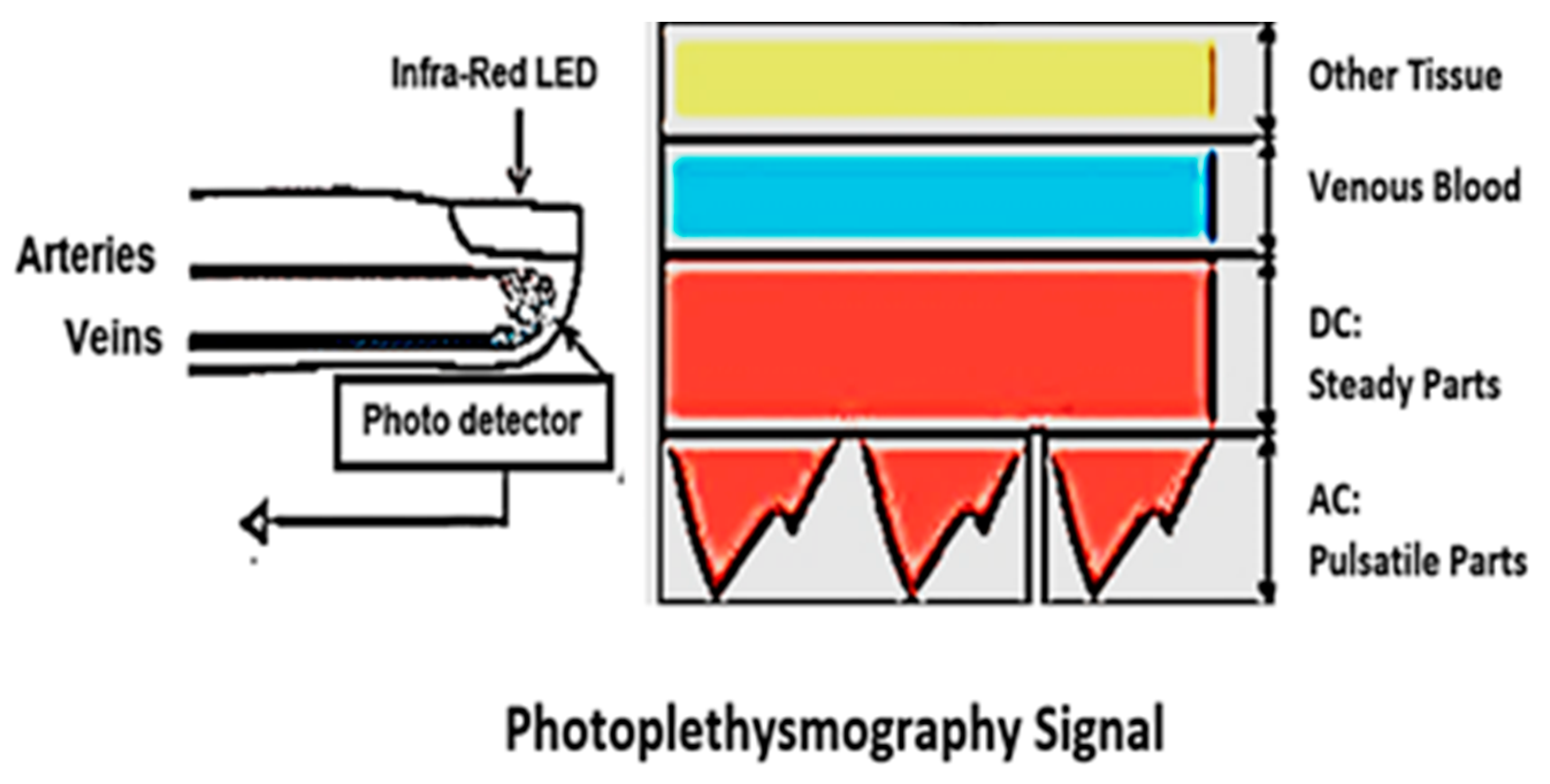
Figure 1. Direct current and alternating current components of the PPG signal due to variation in light absorption.
Information 11 00093 g001
Figure 2. BP simulation using a two-element Windkessel model for SBP/DBP = 160/100 mmHg and HR = 90 bpm parametric models.
Information 11 00093 g002
Figure 3. The PPG features commonly used in prior studies related to BP are the cycle duration (Tc), systolic time (Ts), diastolic time (Td), trough to notch time (Ttn), notch to trough time (Tnt), peak to notch time (Tpn), and the sum of the systolic and diastolic widths at 25% (B25), 33% (B33), 50% (B50), and 75% (B75) of the signal amplitude in each cycle.
Information 11 00093 g003
Figure 4. Three different BP classifications. Each segment consists of 2100 sampling points, corresponding to 2.1 s of data.
Information 11 00093 g004
Figure 5. Skewness characteristics.
Information 11 00093 g005
Figure 6. The PPG waves were categorized into three categories: G1 contains beats with clear systolic and diastolic waveforms with dicrotic notches; G2 contains beats without clear systolic and diastolic waveforms and without dicrotic notches; and G3 contains noisy waveforms.
Information 11 00093 g006
Figure 7. Detailed block diagram of the proposed BP classification technique.
Information 11 00093 g007
Figure 8. (a) Support vector machine, mean testing accuracy: 76.7%; (b) bagged trees, mean testing accuracy: 80%; (c) discriminant analysis, mean testing accuracy: 80%; (d) decision tree, mean testing accuracy: 80%; (e) long short-term memory, mean testing accuracy: 80%; (f) K-nearest neighbor, mean testing accuracy: 87.6%.
Information 11 00093 g008
Figure 9. The coordinates of the points (1200–4100) are scattered according to their respective classifications. There are three classes marked in different colors. Each dataset contains 2100 sample points. Investigated features in the scatter plot for: (a) K = 7; (b) K = 3; and (c) K = 1.
Information 11 00093 g009aInformation 11 00093 g009b
Figure 10. A testing accuracy confusion matrix is used to describe the performance of the classifier in a dataset where the actual values are known.
Information 11 00093 g010
Figure 11. The curve for the training error rate with a varying value of K.
Information 11 00093 g011
Figure 12. Pulse arrival time (PAT) feature.
Information 11 00093 g012
Table 1. Comparison of testing performance.
ClassifierAccuracy
Support vector machine73.6%
Decision tree80.0%
Discriminant analysis80.0%
Bagged trees80.0%
Long short-term memory80.0%
K-nearest neighbor86.7%
Table 2. Comparison K numbers of neighbors.
Number of NeighborsPrediction SpeedTraining TimeAccuracy
7−120 obs/s57.682 s77.3%
5−120 obs/s56.573 s82.1%
3−120 obs/s90.188 s94.5%
1−120 obs/s74.116 s100%
Table 3. Classification performance of KNN algorithm.
TrialTPFPTNFNAccuracy
(%)
Sensitivity
(%)
Specificity
(%)
Recall
(%)
Precision
(%)
F1 Score
(%)
Normal (NT)460590100.00100.00100.00100.00100.00100.00
Prehyper (PHT)33972786.9982.5088.8882.5078.5780.46
Hyper (HT)26779986.7774.2891.8674.2878.7881.09
NT vs. PHT460330100.00100.00100.00100.00100.00100.00
NT vs. HT460260100.00100.00100.00100.00100.00100.00
(NT + PHT) vs. HT79926786.7791.8674.2891.8689.7790.80
Table 4. Classification performance comparison.
MethodTrialFeature ExtractionDatabaseClassifierF1
PAT and PPG Features [26]NT (46 subjects) vs. PHT (41 subjects)
NT (46 subjects) vs. HT (34 subjects)
NT + PHT (87 subjects) vs. HT (34 subjects)
PAT and 10 PPG features121 subjects
(MIMIC database)
AdaBoost Tree74.67%
90.15%
79.71%
PPG Features [26]NT (46 subjects) vs. PHT (41 subjects)
NT (46 subjects) vs. HT (34 subjects)
NT + PHT (87 subjects) vs. HT (34 subjects)
10 PPG
features
121 subjects
(MIMIC database)
AdaBoost Tree72.26%
80.11%
63.76%
PAT Features [26]NT (46 subjects) vs. PHT (41 subjects)
NT (46 subjects) vs. HT (34 subjects)
NT + PHT (87 subjects) vs. HT (34 subjects)
PAT features121 subjects
(MIMIC database)
AdaBoost Tree66.88%
68.04%
53.19%
PAT and PPG Features [26]NT (46 subjects) vs. PHT (41 subjects)
NT (46 subjects) vs. HT (34 subjects)
NT + PHT (87 subjects) vs. HT (34 subjects)
PAT and 10 PPG features121 subjects
(MIMIC database)
Bagged Tree83.88%
94.13%
88.22%
PPG Features [26]NT (46 subjects) vs. PHT (41 subjects)
NT (46 subjects) vs. HT (34 subjects)
NT + PHT (87 subjects) vs. HT (34 subjects)
10 PPG
features
121 subjects
(MIMIC database)
Bagged Tree78.48%
84.98%
75.32%
PAT Features [26]NT (46 subjects) vs. PHT (41 subjects)
NT (46 subjects) vs. HT (34 subjects)
NT + PHT (87 subjects) vs. HT (34 subjects)
PAT features121 subjects
(MIMIC database)
Bagged Tree66.95%
84.98%
75.32%
PAT and PPG Features [26]NT (46 subjects) vs. PHT (41 subjects)
NT (46 subjects) vs. HT (34 subjects)
NT + PHT (87 subjects) vs. HT (34 subjects)
PAT and 10 PPG features121 subjects
(MIMIC database)
Logistic Regression63.92%
79.11%
62.26%
PPG Features [26]NT (46 subjects) vs. PHT (41 subjects)
NT (46 subjects) vs. HT (34 subjects)
NT + PHT (87 subjects) vs. HT (34 subjects)
10 PPG
features
121 subjects
(MIMIC database)
Logistic Regression63.66%
67.94%
47.10%
PAT and PPG Features [26]NT (46 subjects) vs. PHT (41 subjects)
NT (46 subjects) vs. HT (34 subjects)
NT + PHT (87 subjects) vs. HT (34 subjects)
PAT and 10 PPG features121 subjects
(MIMIC database)
KNN83.34%
94.84%
88.49%
Raw PPG Signal [33]NT (46 subjects) vs. PHT (41 subjects)
NT (46 subjects) vs. HT (34 subjects)
NT + PHT (87 subjects) vs. HT (34 subjects)
Continuous Wavelet Transform
(Scalogram)
121 subjects
(MIMIC database)
CNNs80.52%
92.55%
82.95%
Raw PPG Signal
(Proposed method in this study)
NT (46 subjects) vs. PHT (41 subjects)
NT (46 subjects) vs. HT (34 subjects)
(NT + PHT) (87 subjects) vs. HT (34 subjects)
2100 PPG features points121 subjects
(Figshare database)
KNN100%
100%
90.80%
Table 5. Comparison classification performance of KNN.
StudyTrialFeature ExtractionDatabaseSampling FrequencyClassifierF1
Liang.Y et al. [26]NT (46 subjects) vs. PHT (41 subjects)
NT (46 subjects) vs. HT (34 subjects)
NT + PHT (87 subjects) vs. HT (34 subjects)
PAT and 10 PPG features
(two sources: ECG and PPG
121 subjects (MIMIC database)125HzKNN83.34%
94.84%
88.49%
Tjahjadi. H et al.
(Proposed method)
NT (46 subjects) vs. PHT (41 subjects)
NT (46 subjects) vs. HT (34 subjects)
NT + PHT (87 subjects) vs. HT 34 (subjects)
2100 PPG features points (one source: PPG only)121 subjects
(Figshare
database)
1000HzKNN100%
100%
90.90%