A Novel Method for Twitter Sentiment Analysis Based on Attentional-Graph Neural Network

Abstract

Twitter sentiment analysis is an effective tool for various Twitter-based analysis tasks. However, there is still no neural-network-based research which takes both the tweet-text information and user-connection information into account. To this end, we propose the Attentional-graph Neural Network based Twitter Sentiment Analyzer (AGN-TSA), a Twitter sentiment analyzer based on attentional-graph neural networks. AGN-TSA fuses the tweet-text information and the user-connection information through a three-layered neural structure, which includes a word-embedding layer, a user-embedding layer and an attentional graph network layer. For the training of AGN-TSA, dedicated loss functions are designed for the structural controllability of AGN-TSA network. Experiments based on real-world dataset concerning the 2016 presidential election of America exhibit that AGN-TSA is superior under multiple metrics over several prevailing methods, with a performance boost of over 5%. The empirical settings of parameters are given based on extensive rotation experiments.

1. Introduction

Twitter is a well-known social network giant, whose ecosystem has covered a good portion of the populated area on Earth [1]. With such a large number of registered users online, commercial opportunities, management needs and safety concerns on Twitter platform have drawn a lot of attention both academically and industrially. In this situation, the understanding, classification and identification of Twitter users have become important issues to address for Twitter management teams, intelligence agencies and so on. To this end, Twitter sentiment analysis (TSA) came into the spotlight during the last decade, and it has now become an effective tool for Twitter public opinion mining.

In this paper, TSA refers to an analytical task which aims to predict Twitter user sentiment polarity by analyzing the data gathered from the Twitter platform, in order to provide higher-level information for Twitter management operations, to discover underlying trends in public opinion and so on. Research, such as the prediction of election outcomes based on Twitter information [2,3], has validated the value of TSA. Although some ethical concerns about data privacy have induced debates inside both industry and academia, such concerns can be mitigated effectively by leveraging data collected through application programming interfaces (API) [4], which are provided officially by Twitter itself. Meanwhile, when the data collection process abides strictly by the Twitter rules of data collection, and the usage of such data is for proper causes such as building up public-opinion awareness for better management rather than anything related to the infringement of user privacy, ethical problems can be minimized to an acceptable degree.

Traditional methods [2,3,5] based on machine learning take the tweet’s text messages as the input. These works usually use statistical methods to extract features for later analysis, and they are able to achieve decent results (generally above 80% in accuracy). Recent technologies [6,7] adopt various kinds of neural nets for TSA, which are free of hand-crafted features. However, one of the key existing challenges is that all these methods do leverage either tweet-text data or user-connection data, where a fusion-based method, which concerns both kinds of data, is still absent.

To meet the aforementioned challenges, we propose a novel method for TSA based on an attentional-graph neural network—the Attentional-graph Neural Network based Twitter Sentiment Analyzer (AGN-TSA). AGN-TSA mines information from both tweet-text data and user-information data. The core network of AGN-TSA has a three-layered structure, which integrates an embedding layer based on an autoencoder for user embedding, a synthesizing layer based on graph-attention for new representation learning and a prediction layer based on a feed-forward net to predict Twitter user sentiment. An integrated loss function is designed to guarantee end-to-end training of the whole network, which at the same time grants controllability to the overall structure of the network to satisfy different needs. AGN-TSA is tested with a real-world dataset concerning the 2016 presidential election in America, where empirically-optimized parameter settings are searched, and the experiment results show that AGN-TSA outperforms in comparison with multiple traditional methods. Our contributions can be summarized in three ways:

• AGN-TSA is a neural-network-based method which takes both the tweet-text data and the user-connection data into account, which to the best of our knowledge is the first time such an attempt has been made.
• We bridge the gap between graph neural networks (GNN) and TSA by designing a three-layered network with an integrated loss function for regularization, which guarantees the structural-controllability to satisfy different needs for analysis.
• AGN-TSA is tested extensively based on a real-world Twitter dataset concerning the 2016 presidential election in America, where empirically-optimized settings for parameters are given.

The rest of this paper is organized as follows: The Section 2 provides a detailed explanation of the feasibility of AGN-TSA, and this section also gives modular and mathematical elaboration on the structure of AGN-TSA, as well as the loss function design. The Section 3 concerns the experiments based on the real-world dataset, where the experiment configuration, the experiment results and corresponding analysis is given in detail. The final section summarizes the whole work and gives a conclusion to our research.

2. Related Works

In this section, we briefly survey the relevant works on Twitter sentiment analysis for a better understanding of the state-of-the-art methods, as well as the current challenges. There are two major aspects to cover, the first one is about some of the existing TSA techniques, and the other concerns the algorithms for use in TSA.

2.1. Related Works Regarding Twitter Sentiment Analysis

In the last decade, the prediction of Twitter-user sentiment has been brought into the spotlight and has received a wide range of attention. Early in 2010, Tumasjan [2] has done message analysis using Linguistic Inquiry and Word Count (LIWC) [8] software for the 2010 German federal election prediction based on over 100,000 Tweet messages. Instead of a specific statistic for conclusion, the experiment results in this paper reveal that Twitter is used a lot for political purposes, and the user Twitter sentiment closely corresponds to the election results. Such research has been carried out with data regarding elections in other areas. Maynard [3] has done opinion mining using the UK election data from Twitter. The author develops a new data representation for sentiment analysis, which is a triplet containing the user, the opinion and the party of the user. For classification, the author leverages an unsupervised approach based on lexicon analysis. The experiment result delivers a prediction precision of 62.2%, which is a considered a promising result at the early stage of research according to the author. Besides, the author has carried out further experiments based on manual annotation, which gives a relatively-better result with a precision of 79%.

Recent research from Hasan [5] provides us with an integrated approach based on sentiment analyzer and machine learning. For the sentiment analyzer, the author considered the TextBlob [9], a customized Word Sense Disambiguation (W-WSD) [10] and The SentiWordNet [11] for comparison. For the classifier, the author leverages the Waikato Environment for Knowledge Analysis (WEKA) [12] software to deliver the classification based on the calculated polarity and subjectivity, using Naïve Bayes Classifier (NBC) [13] and Support Vector Machine (SVM) [14]. The experiment results show that TextBlob and W-WSD are able to achieve better sentiment analysis results than SentiWordNet could under their experiment settings, with accuracies of 76%, 79% and 55% respectively where NBC is the classifier, and 63%, 62% and 53% when SVM is used.

Severyn and his team [6] proposed a Twitter sentiment analysis method using deep convolutional neural networks (CNN). The author maps the tweet messages into a dedicated sentence matrix with concatenated word vectors. Later the author use a deep CNN to process the sentence matrix, with Rectified Linear Unit (ReLU) [15] as non-linearity and max pooling. Besides, Stochastic Gradient Descent (SGD) is used as the optimizer, and $l_2$ norm is adopted for regularization. During the experiment, the author leverages both unsupervised learning and learning on weakly-supervised data, where the latter involves using the distant supervised data for a network weight update. The experiment results show that the best performance could be reached when the network is initialized with a supervised set with accuracies around 70% over most of the tested datasets. The Word2Vec initialization follows with an averaged 1% performance degradation, while the random initialization achieves far worse results.

Later in 2017, Zhang [7] goes further by carrying out multiple experiments on three different attention CNN schemes for TSA. To bridge the gap between three attention CNN methods, a cross-modality consistent regression (CCR) and transfer learning module are adopted. The results show that the proposed method exceeds the state-of-the-art methods in performance. The sentiment embedding and the lexicon embedding are able to achieve better performance than the semantic embeddings, and the proposed model with expanded attention (model 3 in the article) is able to achieve the best performance over various CNN-based techniques, with an accuracy of 88.83%. Further evaluations regarding the F-1 score strengthen the perspective that expanded attention over multiple words can effectively improve the performance of TSA based on CNN, and the transfer-learning mechanism gives an additional performance boost to the proposed method.

Considering the fusion of different information sources for better neural analysis related to Twitter, such topic is discussed in some other fields of interest, such as the work of Xing [16] which addresses the asset allocation problems in financial markets via neural nets based on social-media sentiment, price change and trading volume information. The data to fuse in Xing’s work is represented in a numeric sequential form, and the network for use is a well-modified recurrent network called evolving clustering method and Long Short-term Memory (ECN-LSTM). AGN-TSA differs from the work of Xing in three fundamental aspects—the first difference is about the fields of interest, where ECN-LSTM is a remedy for asset allocation and AGN-TSA is designed for TSA tasks. The second difference lies in the data for fusion, since the data categories fused in AGN-TSA have totally different data structures, and they cannot be put directly into a numeric sequence in our scheme. The reason is that tweet-text data is in pure-text form, while the user-connection data has a graph structure. The last difference is that instead of RNN, AGN-TSA uses a specifically-designed network with three modular neural-net layers with a sophisticated attention mechanism to address the fusion of text data and graph data for TSA.

In the sense of Twitter-related content, all this aforementioned research relies on the analysis of the tweet-text messages themselves, where no connection information between users is involved. It is our basic argument that the mining of environmental information (user-connection information) stands as a key role in TSA works, and a method which could in this scenario fuse both the tweet-text information and user-connection information will surely be needed for thorough TSA work.

2.2. Related Works Regarding Graph Neural Network

In this subsection we focus on recent trending methods which are potential solutions to the analysis of Twitter user sentiment. Keep in mind that, besides the tweet text data, we are also trying to mine information from connection data, which usually in representation is commonly known as the graph data. To begin with, the spectral graph theory [17] is able to map some information from the topology space to the numeric space, which paves the road to the emergence of numeric-analysis-based methods for graph data learning among neural-network researches. In 2013, Bruna [18] introduced the spectral-CNN to common audiences, which brings the graph neural learning to the spotlight. The author proposed the prototype GNN based on spectral graph theory, where a convolutional kernel is the spectral band-pass function, which is able to achieve locality in the graph spectrum. However, this prototype does not have spatial-locality, and it is also computationally intensive and cannot process multi-graph data.

The following researches focus on finding an optimized approximation of the convolutional kernel, so that the heavy burden of computation could be alleviated. Smooth Spectral CNN [19] is proposed in 2015, where the spectral band-pass kernel is substituted with an interpolated weight function based on the notion that the smoothness in frequency is correlated in the locality in space. Later in 2016, Defferrard [20] has proposed ChebNet, which further simplifies the kernel function into a weight function based on Chebyshev polynomials. In 2017, Kipf [21] proposed the graph convolutional network (GCN), which retains only the first polynomial of the kernel in ChebNet, resulting in a linear band-pass kernel function. This move has finally made the GNN a feasible learning tool for common use. In 2018, Veličković [22] introduced the attention mechanism into the GNN architectures, which contains dedicated attention coefficients for use in the convolutional process of the graph learning.

Our work tries to bridge the gap between the current graph neural network and the application to Twitter sentiment analysis. By developing a hybrid architecture to learn meaningful user embeddings and to fuse both tweet-text data and user-connection data together, we are able to disentangle the problem and achieve better results than the state-of-the-art methods could.

3. Methodology Explanation

3.1. Method Viability

Observations on two major aspects are needed to know a person, one is what it says, the other is what it does. While on Twitter, what a user says can be understood as the tweets it generates, while what the user does refers to the interactions the user has with its environment, namely the connections with other users. The tweets which the target account generates are of crucial importance when we try to identify the account. Yet different from a standard natural-language-processing problem, we tried to combine the tweet-text information with the user-connection information. So in our work, the target for the processing of tweet text is to generate viable and efficient embeddings from the original tweets for later use. For this task we adopt an embedding layer based on word2vec to embed the user based on their tweets, whose aim is to get numerical user embeddings while maximally shred out the redundant information from the tweets.

The modeling of the connections between users comes next. There are multiple kinds of interactions among Twitter users, such as retweeting, liking and following. For retweeting, when a user retweets, it creates a new tweet which contains another tweet and some comments on it. When a user follows another user, it adds all the tweets of the followed user to the follower list. Moreover, a user can like a tweet to express their attitude towards the tweet content, though this attitude may have higher-level polarity such as liking for sarcasm. Noting that different interactions represent different stances of the user, we argue that by taking all possible connections into account, together with the original tweets from the user, we are able to capture a major portion of the user-behavioral information.

As is mentioned in the introduction section, AGN-TSA takes both the tweet-text information and the user-connection information into account. GNN techniques [18,19,20,21,22] are a natural solution to such problems. Among which, GAT [22] considers not only the convolution of structural information from neighbour nodes, but it also gives trainable attention weights for how much such information is utilized. However, GAT is yet not a complete solution to TSA, which needs further structural design to fit in the TSA scenario. AGN-TSA counters such problem using a three-layered neural structure, which successfully couples GAT and TSA in our research scenario. This is the logic flow for the reasoning of our work, and the detailed methodology will be introduced in the following subsections.

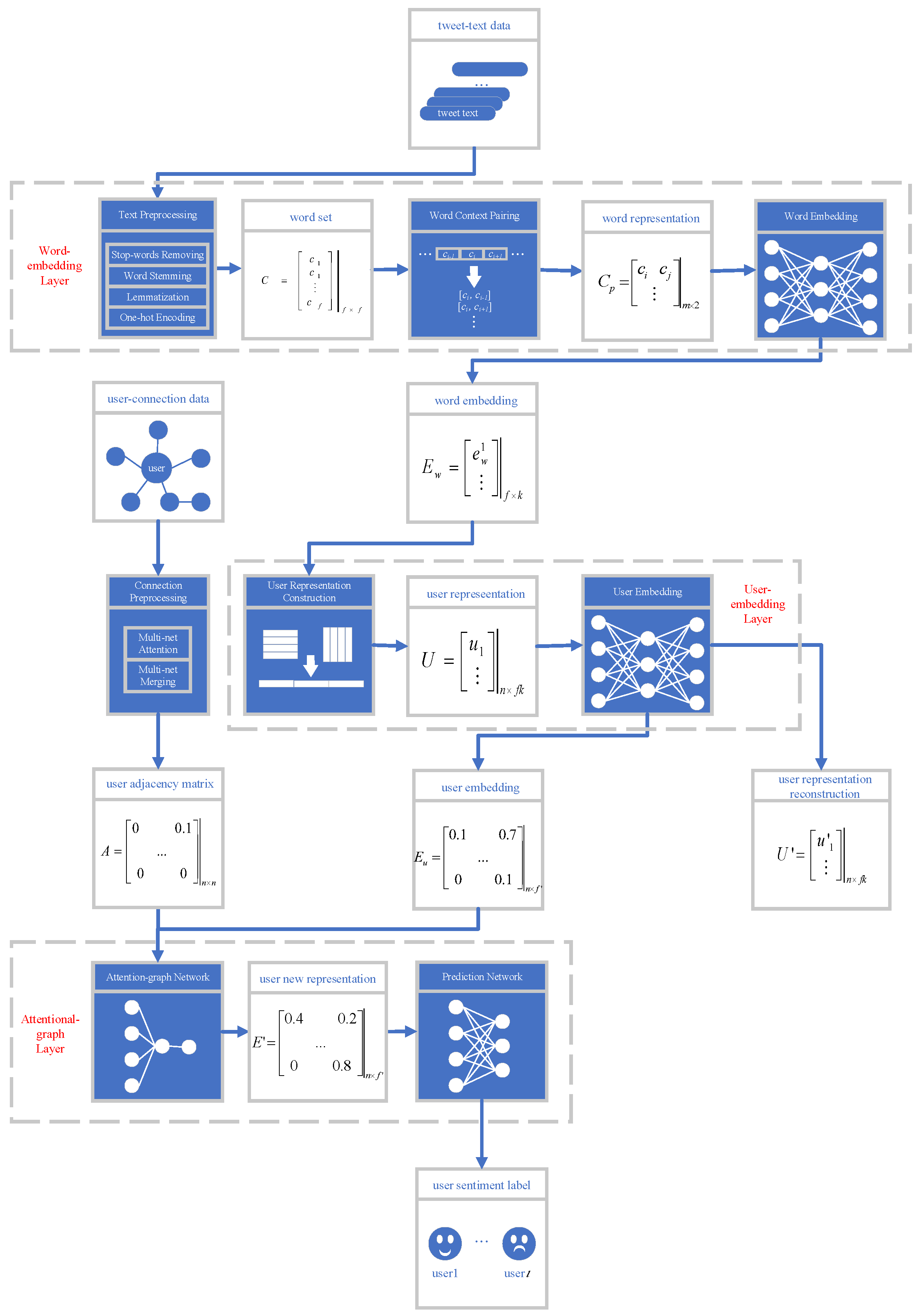
3.2. AGN-TSA Structure

The workflow of the proposed method is shown in Figure 1. From the figure we can see that there are three major layers for the neural network structure—the user embedding layer, the attentional-graph layer and the prediction layer.

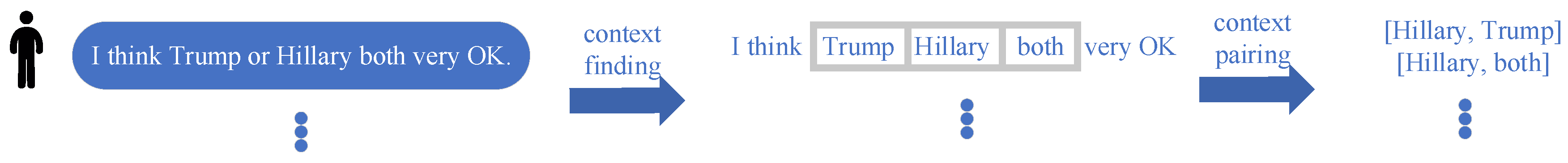
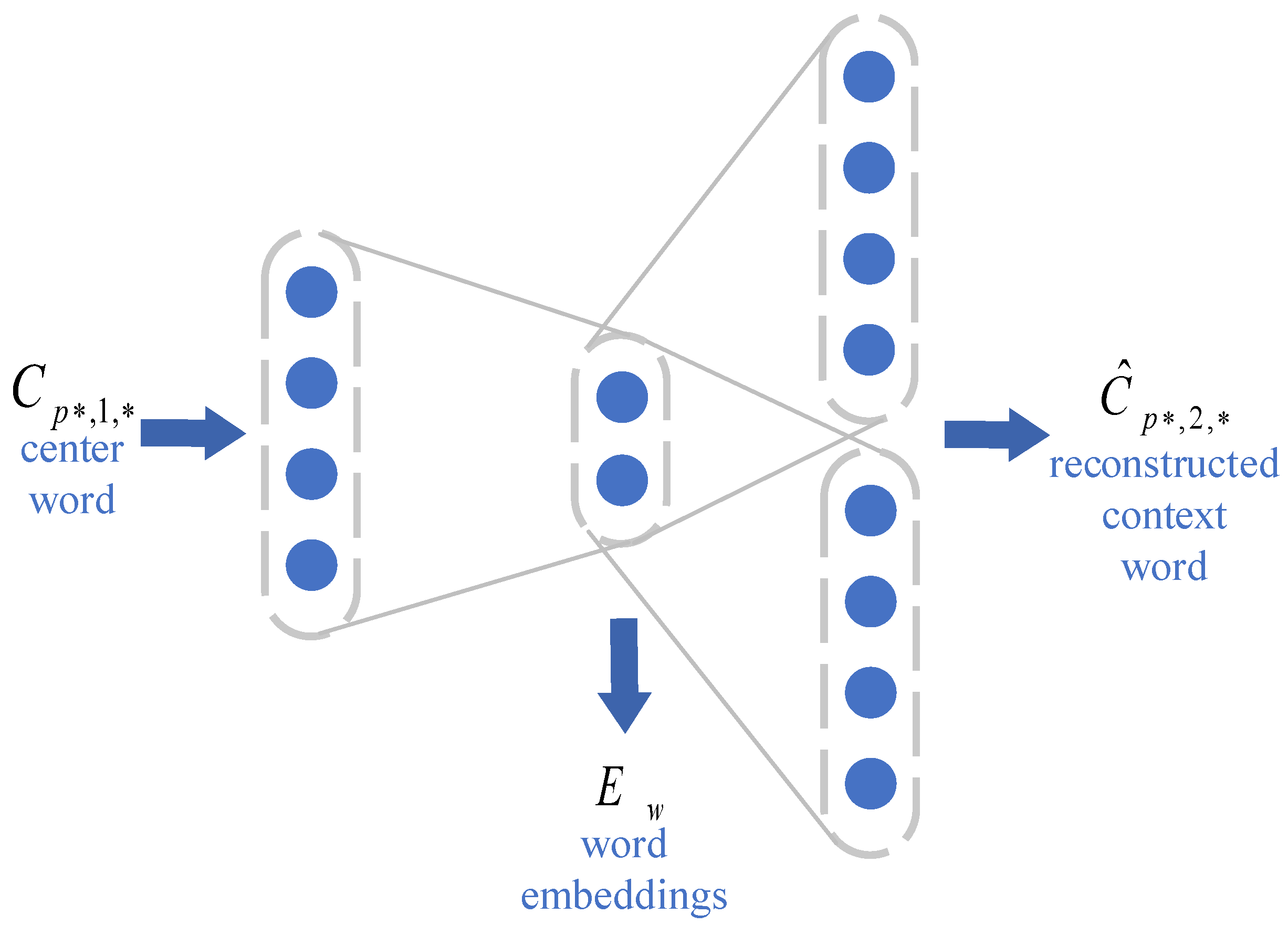
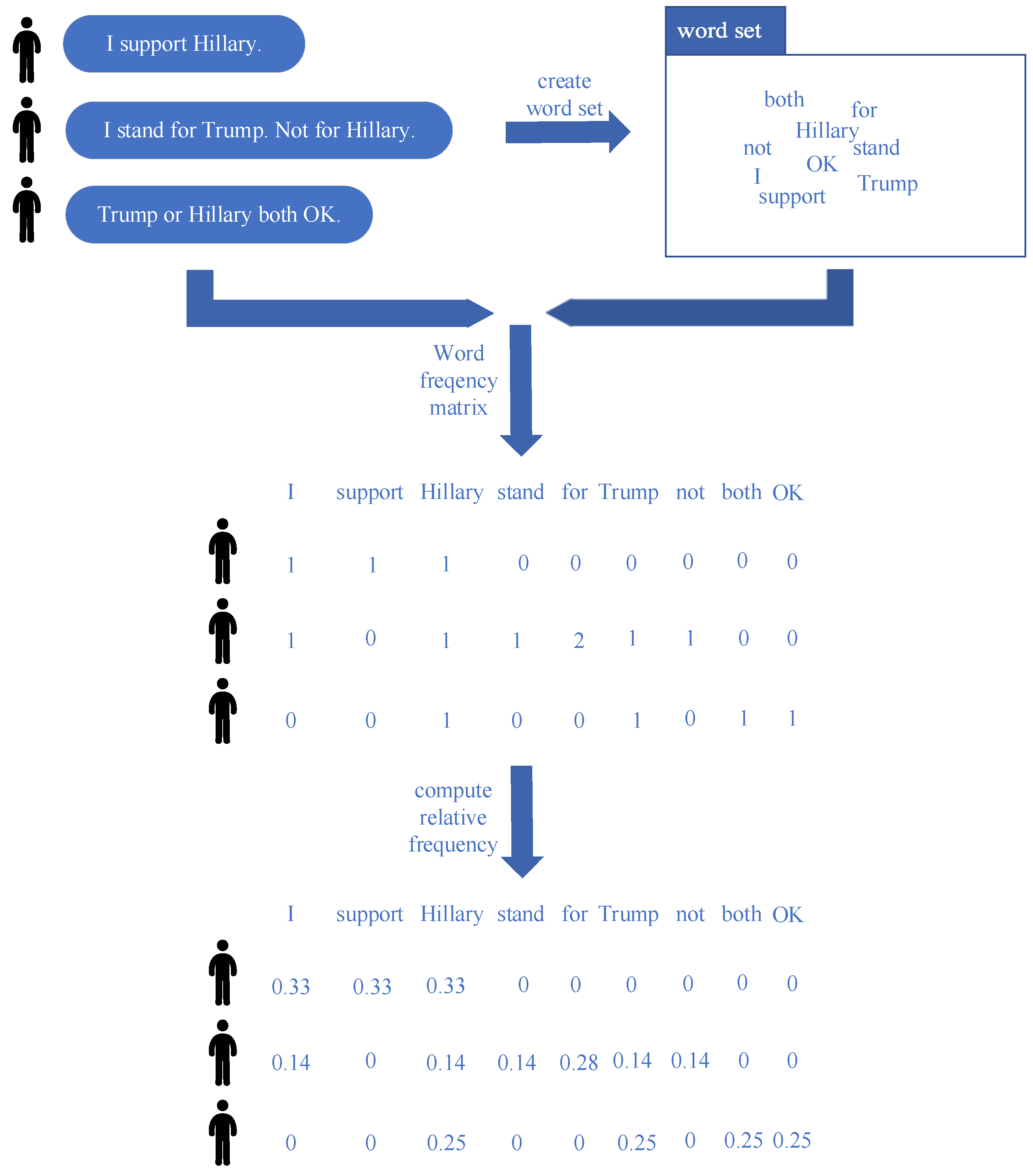
3.2.1. The Word-Embedding Layer

Raw tweet data collected from Twitter is in text form, which neural networks cannot process directly. Besides, raw data is always noisy, which requires corresponding denoising strategies to counter. Thus, preproccessing the data is needed to guarantee the smooth running of AGN-TSA. The preprocessing converts the raw data into feasible data representations as the inputs for latter neural-networks. There are two major tasks for the preprocessing layer, where one is to convert the tweet-text data into numeric representations for neural-network processing, and the other task is to generate integrated user-connection data concerning multiple kinds of user connections.

The preprocessing of tweet-text data consists of stop-words removal [23], word-stemming [24], the lemmatization [25] and vectorization. While the stop-word removing, the word stemming and the lemmatization are standard text-formalization operations to get the basic text form of a word, the vectorization is to convert the text data into a numeric form. In our research, we adopt a word2vec-based method for vectorization. The mathematical explanation is given as follows.

Given the sorted and fixed vocabulary of all investigated users as $C=[c_1,c_2,\dots ,c_f]\in {\mathbb{R}}^{f\times f}$, where $c_i\in {\mathbb{R}}^f$ stands for the one-hot encoding of the ith word inside the word set. The notation f is the total number of word to consider, which is also the input feature number. To quantify the word based on the tweets, word modeling methods are needed, such as the Skip-Gram and continuous bag of words (CBOW). Here in our introduction, we choose the Skip-Gram method as an example to derive the whole process. Denoting the word modeling function as $\mathcal{H}:{\mathbb{R}}^{f\times f}\to {\mathbb{R}}^{m\times 2\times f}$, where m is the number of word representation entries. The word representations $C_p$ can be computed through the simple equation below:

$$C_p=\mathcal{H}\left(C\right).$$

(1)

Let us take the Skip-Gram modeling as an example, and the process is shown in Figure 2. For word $c_i$, we can generate the word-pair entry $[c_i,c_j]$ based on the context of $c_i$, where $c_j$ refers to a word from the context of $c_i$. In this way, $C_p$ can be generated by concerning every word in C. From the computation process we can see that this prototype $C_p$ treats every word-pair entry equally, but some of the entries appear multiple times inside the tweet set, which deserve more attention during learning. Thus, we introduce the weighted word representation $C_p^{\prime }$ to satisfy such needs. Denoting the frequency of appearance for the ith entry $c_p^i$ as $a_{wp}^i\in \mathbb{R}$, thus $a_{wp}=[a_{wp}^1,a_{wp}^2,\dots ,a_{wp}^{1}1]$ refers to the total frequency sequence concerning every context word pair. Noting that $a_{wp}$ is treated as the weight coefficient for the learning of word embeddings, where $C_p^{\prime }$ can be computed through the equation below:

$$\begin{array}{cc}\hfill C_p^{\prime }& =a_{wp}\circ C_p\hfill \\ \hfill & =[a_{wp}^1{c}_p^1,a_{wp}^2{c}_p^2,\dots ,a_{wp}^m{c}_p^m],\hfill \end{array}$$

(2)

where the notation ∘ refers to the Hadamard production between two vectors. After obtaining $C_p^{\prime }$, we can now start to compute the word embeddings based on a butterfly-shaped neural network, which is shown in Figure 3. The function which converts $C_p^{\prime }$ into word embeddings $E_w$ is denoted as $\mathcal{E}:{\mathbb{R}}^{m\times 2\times f}\to {\mathbb{R}}^{f\times k}$, where k refers to the word embedding length. $\mathcal{E}$ is an encoding network with reducing neuron count as the neural layer goes deeper. For each entry in $C_p^{\prime }$, $\mathcal{E}$ takes the first word in this entry as input and output the embedding of this word. For the whole set, the process can be described in the equation below:

$$E_w=\mathcal{E}(C_{p\ast ,1,\ast }^{\prime }),$$

(3)

where $C_{p\ast ,1,\ast }^{\prime }$ denotes the first plane regarding the second dimension of $C_p^{\prime }$. $E_w$ is used to reconstruct $C_{p\ast ,2,\ast }^{\prime }$ through a neuron-increasing series of neural layers, which is denoted as $\mathcal{D}:{\mathbb{R}}^{f\times k}\to {\mathbb{R}}^{m\times n\times f}$. Concerning the whole set, the process is shown in the equation below:

$$\begin{array}{cc}\hfill {\widehat{C}}_{p\ast ,2,\ast }^{\prime }& =\mathcal{D}\left(E_w\right)\hfill \\ \hfill & =\mathcal{D}(\mathcal{E}(C_{p\ast ,1,\ast }^{\prime })),\hfill \end{array}$$

(4)

where ${\widehat{C}}_{p\ast ,2,\ast }^{\prime }$ refers the reconstruction of $C_{p\ast ,2,\ast }^{\prime }$. Noting that ${\widehat{C}}_{p\ast ,2,\ast }^{\prime }$ is computed in order to measure its difference from $C_{p\ast ,2,\ast }^{\prime }$, which is used as the loss function for the update of parameters in $\mathcal{E}$ and $\mathcal{D}$ (which will be covered in the back propagation section). Until now, the word-embedding layer is finished.

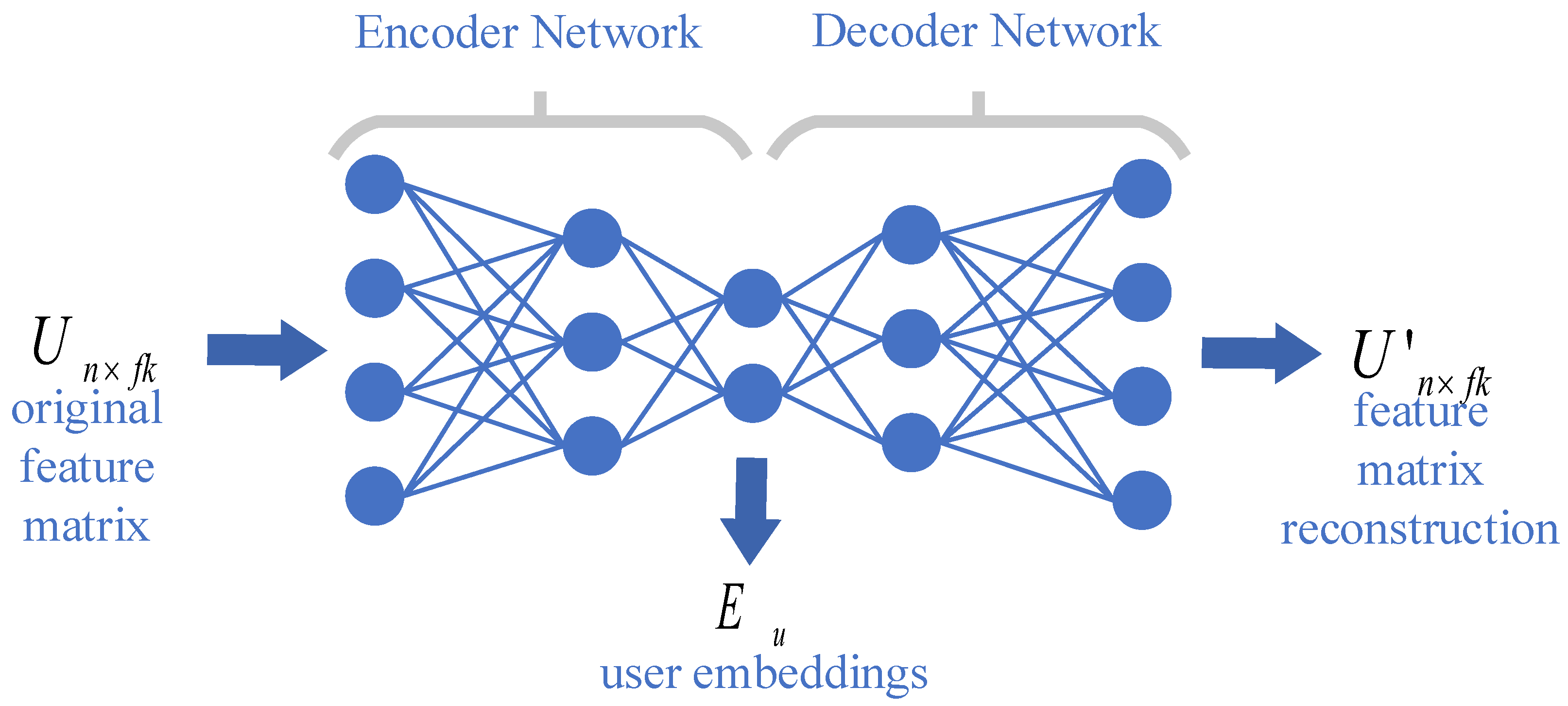
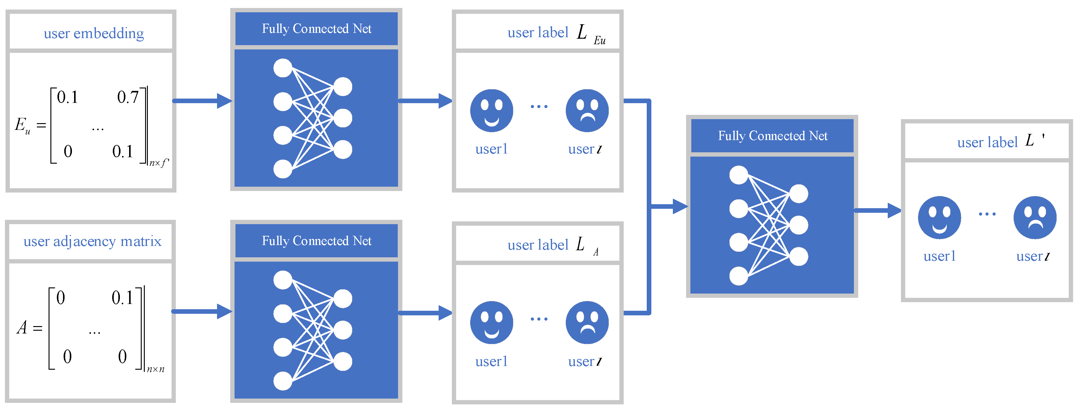
3.2.2. The User-Embedding Layer

The user embedding layer converts the tweet-text data representation into user embeddings according to the word embeddings from the previous layer. After obtaining $E_w$, The following task is to generate user representations $U=[u_1,u_2,\dots ,u_n]\in {\mathbb{R}}^{n\times fk}$, where n refers to the number of users. For user i, a word frequency sequence $c_{freq,i}=[c_{freq,i}^1,c_{freq,i}^2,\dots ,c_{freq,i}^f]\in {\mathbb{R}}^f$ is generated, where $c_{freq}^i$ refers to the frequency of the ith word. $u_i$ is generated through the following equation:

$$u_i=\mathtt{concat}(c_{freq,i}\circ E_w),$$

(5)

where operation $\mathtt{concat}$ is a concatenation operation to generate a long sequence from multiple short sequences. As we can see, $u_i$ has a length of $fk$, which is usually much higher than that of C, since k is commonly larger than 1. Since most of the users do not cover the whole vocabulary C in their tweet set, $u_i$ would always be highly-sparse. To counter these problems, we introduce an autoencoder network to embed $u_i$ into a dense space, where the redundant information inside $u_i$ could be maximally cut out, while useful information could be optimally retained. The process of the autoencoder is shown in Figure 4. Denoting this encoder part of this autoencoder as $\mathcal{A}:{\mathbb{R}}^{fk}\to {\mathbb{R}}^{f^{\prime }}$, where $f^{\prime }$ refers to the length of the user embeddings $E_u=[e_u^1,e_u^2,\dots ,e_u^n]\in {\mathbb{R}}^{n\times f^{\prime }}$. The process is shown in the following equation:

$$E_u=\mathcal{A}\left(U\right).$$

(6)

Following the encoder network, a decoder network follows to try to reconstruct U, where the reconstruction is denoted as $U^{\prime }$. The purpose of this decoder is to create $U^{\prime }$, where the difference between U and $U^{\prime }$ could be measured, and the network could be optimized towards minimizing the difference. Similar to the encoder denotation, we denote the decoder part of this autoencoder as $\mathcal{B}:{\mathbb{R}}^{f^{\prime }}\to {\mathbb{R}}^{fk}$, and the process is shown in the following equation:

$$\begin{array}{cc}\hfill U^{\prime }& =\mathcal{B}\left(E_u\right)\hfill \\ \hfill & =\mathcal{B}\left(\mathcal{A}\right(U\left)\right).\hfill \end{array}$$

(7)

By Reaching $E_u$ and $U^{\prime }$, the user-embedding layer is finished.

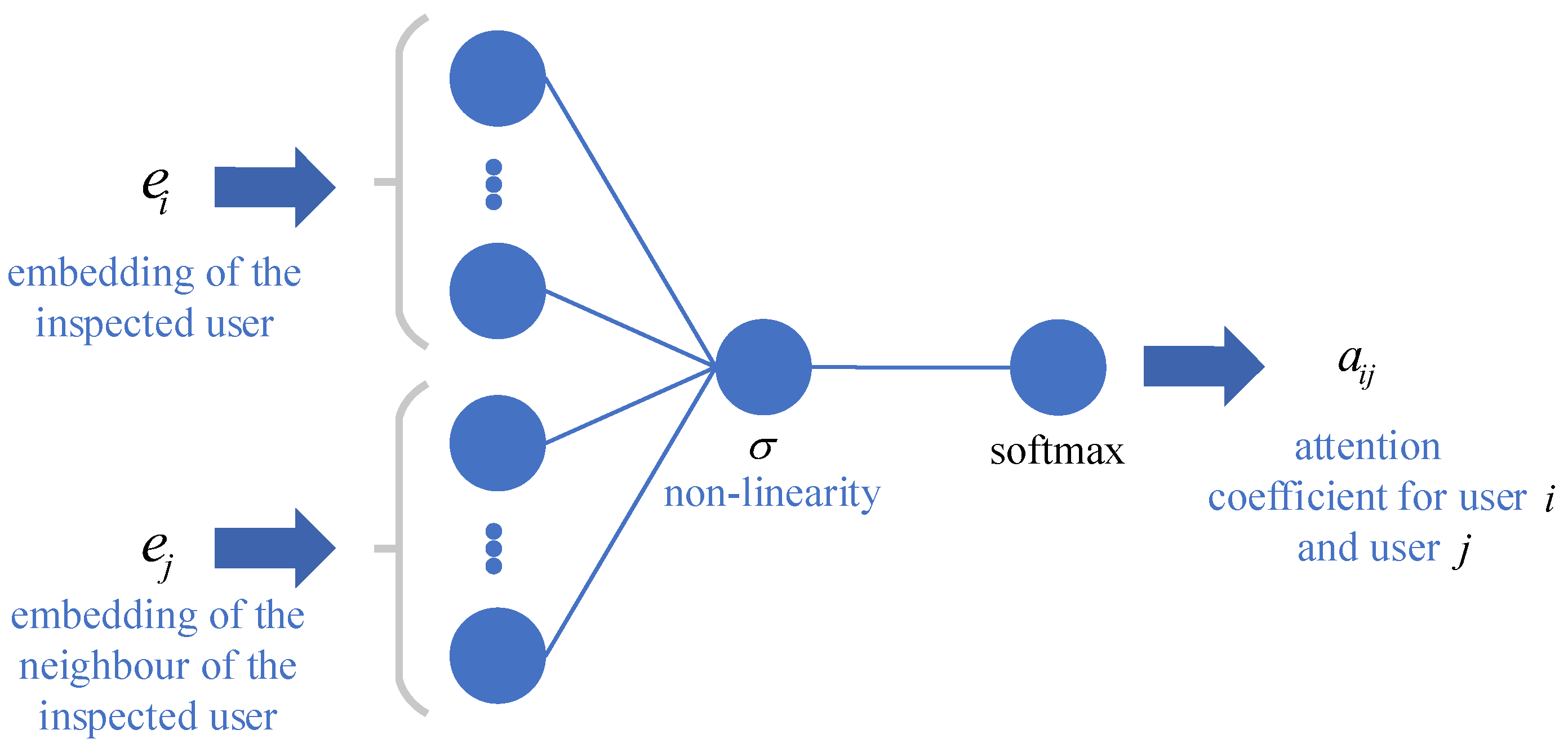
3.2.3. The Attentional-Graph Layer

The user embedding $E_u$ is a good representation of the tweet-text information, but it contains no user-connection information. Following the embedding layer, the attentional-graph layer kicks in, which fuses the user embedding and the connection data together, and generate the new user representation which contains both the tweet-text information an the user-connection information. We leverage an integrated representation based on adjacency matrix for the user-connection data under multiple connection categories. Denoting the adjacency-matrix vector as $A^{\prime }=[A_1,A_2,\dots ,A_v]\in {\mathbb{R}}^{v\times n\times n}$, where v denotes the number of interaction’s category. The combined adjacency matrix with attention $A\in {\mathbb{R}}^{n\times n}$ can be defined with the equation below:

$$\begin{array}{cc}\hfill A& =a_{adj}•A^{\prime }\hfill \\ \hfill & ={\displaystyle \sum _{i=1}^k}{a}_{adj}^1{A}_1,\hfill \end{array}$$

(8)

where $a_{adj}=[a_{adj}^1,a_{adj}^2,\dots ,a_{adj}^v]\in {\mathbb{R}}^v$ stands for the attention coefficients for adjacency matrix, which will be optimized alongside the training of the neural network. Till now, the adjacency matrix and the feature matrix are all prepared for use. With $E_u$ and A, we can derive the mathematical equations for the attentional-graph layer. For a user in the connection graph, the graph-attention layer generates a new representation for this user by integrating its neighbour information with its own information using an attention mechanism. The core conception beneath the attention mechanism is to find out how much the neighbours contribute to the prediction of the core node, which is to compute the attention coefficients between considered node and its neighbours. Denoting the embedding for user i as $e_i$, and the neighbour set of user i as $N_i$ (including user i itself). Denoting the attention coefficient for user i to its neighbour user j as $a_{ij}$, the computation of $a_{ij}$ is reached through a neural network denoted as $\mathcal{G}:{\mathbb{R}}^{2f^{\prime }}\to {\mathbb{R}}^{f^{\prime }}$ defined in the equation below:

$$a_{ij}=\mathcal{G}(e_i,e_j),$$

(9)

where $\mathcal{G}$ contains a $\mathtt{concat}$ operation, a single-layered feed-forward network and a softmax layer, thus we can expand Equation (9) into a more detailed version:

$$\begin{array}{cc}\hfill a_{ij}& =\mathtt{softmax}\left(\sigma \left(W(e_i,e_j)\right)\right)\hfill \\ \hfill & =\frac{\mathtt{exp}\left(\sigma \left(\alpha \left(\mathtt{concat}(e_i,e_k)\right)\right)\right)}{{\sum }_{k\in N_i}\mathtt{exp}\left(\sigma \left(\alpha \left(\mathtt{concat}(e_i,e_k)\right)\right)\right)},\hfill \end{array}$$

(10)

where $\sigma$ refers to the nonlinearity (Leaky ReLU for example) operation, and $\alpha$ is the network parameter to train. Again, the operation $\mathtt{concat}:{\mathbb{R}}^{f^{\prime }}\times {\mathbb{R}}^{f^{\prime }}\to {\mathbb{R}}^{2f^{\prime }}$ concatenate two weighted embeddings into a long vector for network input. The computation process for $a_{ij}$ is shown in Figure 5. Until now, the new representation $e_i^{\prime }$ of user i can be reached through an arithmetic averaging over all its neighbours:

$$e_i^{\prime }=\frac{1}{k}\sum _{j\in N_i}{a}_{ij}{e}_j.$$

(11)

After this, the new representation of the total user set $E^{\prime }=[e_1^{\prime },e_2^{\prime },\dots ,e_k^{\prime }]$ can be thus obtained. Now we have obtained the final representation $E^{\prime }$ for the users, the final task is to predict the user labels $L^{\prime }\in {\mathbb{R}}^c$ with $E^{\prime }$, where c indicates the number of the label category. We leverage a fully-connected net $\mathcal{P}:{\mathbb{R}}^{f^{\prime }}\to {\mathbb{R}}^c$ to achieve the prediction.

$$L^{\prime }=\mathcal{P}\left(E^{\prime }\right).$$

(12)

Note that reaching $L^{\prime }$ means the end of the forward pass of AGN-TSA. In our design, the purpose of the forward pass in AGN-TSA is to compute $U^{\prime }$ and $L^{\prime }$, as well as to update the parameters inside the network based on the computed loss function from $U^{\prime }$ and $L^{\prime }$, which will be stated in the next subsection.

3.3. The Back Propagation Process

The major issue in the back propagation process is to design a viable loss function to update the parameters of the network during training. For optimization, there are two major part of this network which will be optimized separately. The first part is the word-embedding network, and the other part is the user-embedding network and the attentional-graph network. The reason for isolating the word-embedding network is that an optimized word embedding $E_w$ is essential for constructing the user representation U, which requires a fully-trained word-embedding network to compute. For the word-embedding network training, we use the cross entropy between ${\widehat{C}}_{p\ast ,2,\ast }^{\prime }$ and $C_{p\ast ,2,\ast }^{\prime }$ as the loss function. Denoting the ground truth probability of word i as $p_w^i$, and the predicted probability of word i as ${\widehat{p}}_w^i$, the cross entropy for word-embedding network ${\mathsf{\Phi }}_w:{\mathbb{R}}^{f\times k}\times {\mathbb{R}}^{f\times k}\to \mathbb{R}$ is shown in the equation below:

$${\mathsf{\Phi }}_w(C_{p\ast ,2,\ast }^{\prime },{\widehat{C}}_{p\ast ,2,\ast }^{\prime })=-{\displaystyle \sum _{i=1}^l}{p}_w^i\mathtt{log}({\widehat{p}}_w^i).$$

(13)

As for the loss function for the user-embedding and the attentional-graph layer, we consider the mean-square error $\Theta :{\mathbb{R}}^{fk}\times {\mathbb{R}}^{fk}\to \mathbb{R}$ (MSE) between the original user representation U and the reconstructed user representation $U^{\prime }$ for the user embedding network, which is defined in the equation below:

$$\Theta (U,U^{\prime })=\frac{1}{fk}{\left({\parallel U-U^{\prime }\parallel }_2\right)}^2.$$

(14)

For the prediction process, again we adopt the cross Entropy ${\mathsf{\Phi }}_l:{\mathbb{R}}^c\times {\mathbb{R}}^c\to \mathbb{R}$ to quantify the difference between the predicted label $L^{\prime }$ and the ground truth L. Similar to the definition of $\mathsf{\Phi }$, denoting the ground truth probability of user i as $p_i$ and that of the predicted label as $p_i^{\prime }$, the cross entropy can be defined in the equation below:

$$\Omega (L,L^{\prime })=-{\displaystyle \sum _{i=1}^l}{p}_i\mathtt{log}\left(p_i^{\prime }\right).$$

(15)

Thus, the joint optimization objective $\Gamma :{\mathbb{R}}^{fk}\times {\mathbb{R}}^{fk}\times {\mathbb{R}}^c\times {\mathbb{R}}^c\to \mathbb{R}$ can be reached as the weighted sum of $\Theta (F,F^{\prime })$ and $\Omega (L,L^{\prime })$, as is shown in equation below:

$$\begin{array}{cc}\hfill \Gamma (U,U^{\prime },L,L^{\prime })& =\theta \Theta (U,U^{\prime })+\Omega (L,L^{\prime })\hfill \\ \hfill & =\frac{\theta }{fk}(\parallel U-U^{\prime }{{\parallel }_2)}^2-{\displaystyle \sum _{i=1}^l}{p}_i\mathtt{log}\left(p_i^{\prime }\right),\hfill \end{array}$$

(16)

where $\theta$ refers to the weight of the MSE term $\Theta (F,F^{\prime })$, noting that $\theta$ can be treated as the controller for the user-embedding network. When $\theta =0$, the parameters in the reconstruction part of the user-embedding network will not get updated during the training, since the MSE term in the optimization objective is disabled. In this situation, the user-embedding network will become a simple feed-forward network, where the learned embeddings are no longer guaranteed to be input-reconstructable. Considering that our method is designed for prediction tasks, we set the weight of the cross-entropy term to be permanently 1. Again, please bear in mind that ${\mathsf{\Phi }}_w$ an $\Gamma$ will be optimized separately.

4. Experiments and Analysis

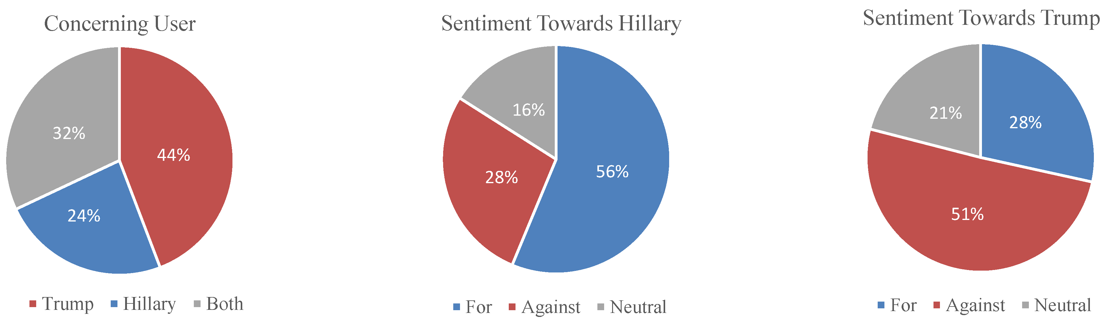
4.1. Experiment Configuration

In this experiment, we try to evaluate our methods based on a real-world dataset. The prediction target is the user sentiment towards the two major presidential candidates during the 2016 presidential election in America—Hillary Clinton and Donald Trump. The complete label categories and their explanations are shown in

Table 1. The categories for twitter user sentiment analysis.

Category Name	Category Explanation
Hillary_for	Most of the user’s tweets have positive attitude towards Hillary Clinton.
Hillary_neutral	No prominent attitude towards Hillary Clinton has been found.
Hillary_against	Most of the user’s tweets have negative attitude towards Hillary Clinton.
Trump_for	Most of the user’s tweets have positive attitude towards Donald Trump.
Trump_neutral	No prominent attitude towards Donald Trump has been found.
Trump_against	Most of the user’s tweets have negative attitude towards Donald Trump.

. From Table 1 we can see that there are two sets of categories, where the first three categories concerns the sentiment towards Hillary Clinton, and the others concerns those towards Donald Trump. As a result, the experiments will be done on these two sets separately.

The dataset involved in this paper was collected legitimately by our research team during the 2016 presidential election in America, through the APIs were officially provided by Twitter itself. It took a consistent capture which lasted for over two months to build up this dataset. All the captured tweets and user profile pages were publicly accessible back then during our capture. More than three years have passed, though some of the tweets might be deleted, and some of the accounts might be terminated due to various reasons, we believe that there should be a good portion of tweets or user pages which are still accessible, which makes it quite possible to trace back the original user according to the tweet content even if the dataset is anonymized. Thus, for the avoidance of potential privacy infringement, our research team decided not to share the dataset involved in this paper.

The raw dataset is very noisy since there is quite a portion of users who have not expressed any opinion concerning the 2016 presidential election of America. Thus, we selected 1224 users with mutual connections between each other from the raw dataset. Since AGN-TSA requires both tweet-text data and user-connection data to run, there are two criteria for the user selection to guarantee both kinds of data are present. One is that during the monitoring period, these selected users have at least once expressed their political sentiment towards the aforementioned presidential candidates, so that the selected users all have their own candidate-related tweets. The second criterion is that during the monitoring period, each selected user has at least once interacted with another user who is also in this dataset, whether liking, following or retweeting, so that all the selected users could be covered in the user-connection data.

Regarding the ground truth of this dataset, to guarantee a relatively-high accuracy, all the ground-truth labels are annotated manually by our research crew after going through all the content the users generated in this dataset. For example, a user is annotated as “For Hillary” if a majority of their election-related tweets during the monitoring period have positive sentiment towards Hillary Clinton. The ground truth user composition is shown in Figure 6. The total number of our annotators involved in this task is 108, and a majority of them are graduate students in our lab, while the others are undergraduate interns. Each user is annotated by at least three annotators, where any dispute about the label will be decided through sufficient discussions among the annotators, so that each user has only one ground-truth label for each prediction target.

For the word-embedding layer, there are multiple methods for modeling the tweet-text data. In the introduction we choose the Skip-Gram method as an example, however other prevailing methods such as CBOW are also viable choices. So to find out an empirically-optimized method for word-modeling in AGN-TSA, We compare the performance of AGN-TSA under different word-modeling methods, which include the Skip-Gram, CBOW and pure autoencoder. While we cover no excessively elaboration of the CBOW mechanism, which is quite similar with Skip-Gram, the word-modeling with autoencoder is shown in Appendix A at the end of this paper.

For the construction of the adjacency matrix, we build undirected graphs from the connection data. The edge value between two users are the frequency of connections during our monitoring period. For the denoising of the tweet-text data, the retained-word count f is also a critical parameter to attend to. the retained-word count f refers to the number of retained words to consider when we build our original input for embedding layer, and it will be concerned in our experiments.

In order to exhibit the power of our method, we also carried out contrasting experiments with some of the traditional machine learning algorithms, which includes Naïve Bayes Classifier (NBC), Decision Tree (DST), Support Vector Machine (SVM) and Random Forest (RDF). Moreover, since AGN-TSA is a framework where the data fusion happens at the embedding stage (at the attentional-graph layer), another experiment is added where AGN-TSA is compared with another framework whose fusion occurs at the decision stage. This decision-stage-fusion framework (DSF) is explained in detail in Appendix B at the end of this paper. For the purpose of getting a thorough evaluation, The metrics we use in our experiments for comparison are accuracy, precision, recall and F1-score.

4.2. Experiment Results and Analysis

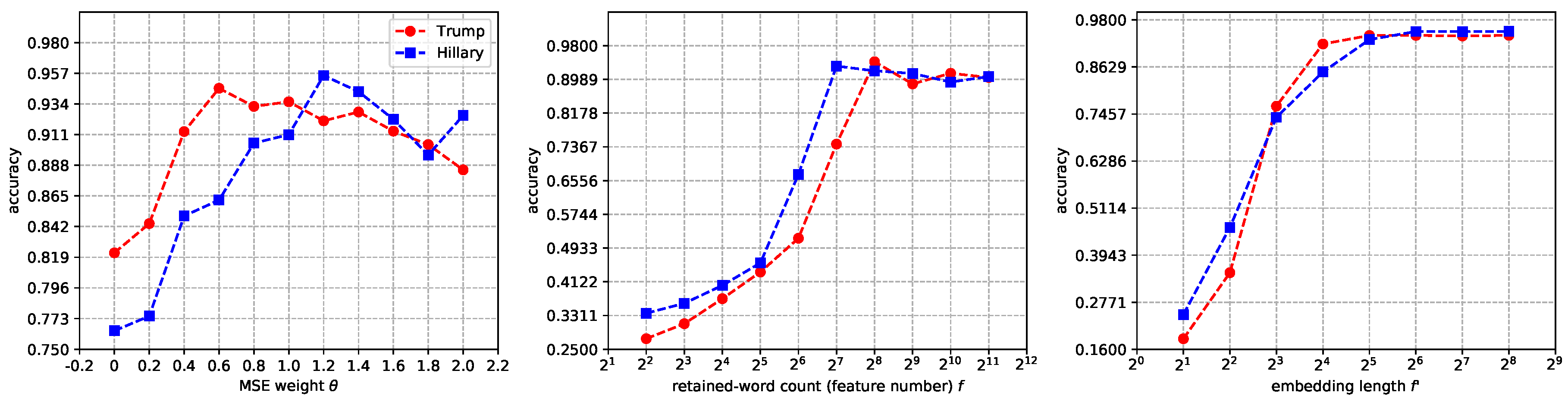
4.2.1. Parameter Rotation Experiment

The first set of experiments we have conducted are the parameter-rotation experiments. In these experiments, we rotate on several key parameters and try to get empirically-optimized settings for these parameters. The parameters to rotate includes the MSE weight $\theta$, the retaining words count f and the embedding length $f^{\prime }$. For these experiments, we use the accuracy as the evaluation metric. The results are shown in Figure 7.

From the sub-figure located in the left side of Figure 7, we can see that as $\theta$ increases, the accuracy shows an growing tendency at the beginning. After reaching a maximum value, the accuracy starts to decrease turbulently. This peak-shape curve is spotted both in the Hillary experiment and the Donald experiment, though their $\theta$ values for maximal accuracy are different. This validates the contribution of the reconstruction network in the embedding layer, where the accuracy is greater than that when it is just a feed-forward network (when $\theta =0$). However, we can notice that if $\theta$ grows too big, the reconstruction network is overly emphasized, where the training would put too much attention on updating the values of the reconstruction network, and the overall prediction task is less attended. Based on our observation, we suggest to set $\theta$ to be somewhere between 0.5 and 1.5.

For the experiment on the retained-word count f (also known as the input feature number), from the figure we can see that as f increase exponentially, the accuracy curve goes a slow increase at the beginning, while at the middle the curve goes up faster and after reaching a maximum, the accuracy starts to decrease very slowly and turbulently. The slow start is an indication that the most-commonly used words are not good choices for classification, since that everyone is using it also means that it is not discriminative. The rapid increase in accuracy after the slow start also validate such a claim, the rare usage of words may increase the performance in classification tasks. However, since the increase of f also adds up to the scale of the embedding layer, which brings heavier burden to the training process. Once the optimization puts more effort to the updating of the embedding layer parameters, the overall prediction-oriented optimization will be diluted, and the overall accuracy will stop increasing or even start to decrease, as is observed in our experiments. Thus, we suggest to choose a mid-ranged number for the retained-word count f, where it is between $2^6$ and $2^8$ in our experiments.

Finally, concerning the embedding length $f^{\prime }$, the experiments gives us a converging curve, where as the neurons in embedding layer keep increasing, the accuracy also goes up monotonically with a decreasing speed. As the embedding length getting longer, more user information is retained inside the embedding, and the prediction can get more useful information for classification, which leads to higher accuracy. Nevertheless, the long embedding length will again increase the burden of the training, which slows down the overall prediction process and makes the optimization more consuming both temporally and spatially. So based on our observation, feasible value for $f^{\prime }$ should be set to somewhere between $2^4$ and $2^5$.

4.2.2. Word-Embedding Method Experiment

As is mentioned in the previous section, we consider optimizing the choice of method for word modeling during the word-embedding process. The choice we consider are three—Skip-Gram, CBOW and pure autoencoder. We test the settings for all four metrics which are mentioned early in this paper, and the results are shown in

Table 2. Performance comparison between three word-modeling methods.

Method	Sentiment Towards Trump				Sentiment Towards Hillary
	Accuracy	Precision	Recall	F1-Score	Accuracy	Precision	Recall	F1-Score
autoencoder	0.7692	0.7705	0.7692	0.7697	0.7462	0.7486	0.7462	0.7471
CBOW	0.8615	0.8645	0.8615	0.8615	0.8692	0.8696	0.8692	0.8682
Skip-Gram	0.9462	0.9467	0.9462	0.9457	0.9539	0.9557	0.9539	0.9536

. From the table we can clearly see that Skip-Gram is a better choice here, with a performance boost of 8% over CBOW and 17% percent over pure autoencoder. The reason behind this phenomenon is that Skip-Gram is a method which performs well for modeling the rare words. Fortunately, as is shown in our last experiment, rare words are good choices for our prediction, and this is why the Skip-Gram gets to shine in this set of experiments. The more rare words we choose, the better the performance of Skip-Gram, and the better the prediction results. Though CBOW is also a good modeling method, but it does not quite stand out for this scenario. While for pure autoencoder, the results are the worst, which could be explained by the nature of this modeling: it contains no context information in the generated word embeddings, which leads to a low prediction accuracy.

4.2.3. Method Contrasting Experiment

Another set of experiments we deliver is the method contrasting experiments. In these experiments, the traditional methods use the user representation U as feature for input. The results are shown in

Table 3. Performance comparison between AGN-TSA and traditional methods.

Method	Sentiment Towards Trump				Sentiment Towards Hillary
	Accuracy	Precision	Recall	F1-Score	Accuracy	Precision	Recall	F1-Score
NBC	0.8385	0.8391	0.8385	0.8387	0.8076	0.8107	0.8077	0.8082
DCT	0.8769	0.8782	0.8769	0.8773	0.8462	0.8491	0.8462	0.8460
SVM	0.8923	0.8934	0.8923	0.8926	0.8692	0.8704	0.8692	0.8686
RDF	0.8846	0.8885	0.8846	0.8852	0.8769	0.8799	0.8769	0.8765
DSF	0.9077	0.9080	0.9077	0.9076	0.9154	0.9168	0.9153	0.9158
AGN-TSA	0.9462	0.9476	0.9462	0.9463	0.9539	0.9550	0.9539	0.9538

. we can see that the traditional methods are able to achieve decent performance, but AGN-TSA is able to achieve better results than the tradition methods does over all metrics. One reason for such an outcome is that our method fuses both the tweet-text data and user-connection data for better results. So in comparison with the feature-only methods, AGN-TSA is able to take advantage from the user-connection information for better performance. This idea is further validated with the outcome of DSF, who also leverages the user-connection information to strengthen the prediction.

Regarding the comparison between the results of DSF and AGN-TSA, we can see that AGN-TSA is able to achieve better results with all metrics 4% higher than those of DSF. This difference is introduced mainly by the usage of the user-connection data. As we know, each row of the adjacency matrix stands for the connection one user has to all the users, and a connection value between two users alone does have indication for the user sentiment, but this indication is not strong. So when the decisions from two different predictors are fused, the prediction based on the user-text information would win over the other side most of the time, which renders the user-connection part frequently inactive. This claim is validated by the fact that DSF has a limited performance boost over the traditional methods, as is shown in Table 3. Instead, intuitively speaking, AGN-TSA leverages the user-connection data as the clue to improve the embeddings of the users, as is stated in the methodology section. In this way, the user-connection information is always actively leveraged for better prediction, which results in a better performance than DSF could achieve.

5. Conclusions

This paper proposes AGN-TSA, a Twitter sentiment analyzer based on Attentional-Graph neural network. AGN-TSA is the first neural framework proposed to leverage both tweet-text data and user-connection data for TSA tasks, where we bridge the gap between GNN and TSA by coupling the word-embedding network and attentional-graph network together through a user-embedding network. Beside, by designing a three-layered network structure and dedicated loss functions, the structural controllability over AGN-TSA could be achieved. Notably, all the data involved in this paper is collected legitimately according to terms of usage for Twitter API, and the purpose of AGN-TSA is to improve situation awareness of public opinion for better management. Usages of AGN-TSA which might induce any infringement of user privacy should be stopped for both ethical and legal reasons.

Regarding the parameter rotation experiments, empirically-optimized settings are found based on experiment settings. For the MSE weight coefficient $\theta$, a value between 0.5 to 1.5 is ideal. For the retained-word count f, optimal value locates between $2^6$ to $2^8$. While for the user embedding length $f^{\prime }$, we suggest a value between $2^4$ to $2^5$. Later in the word-embedding method experiments, Skip-Gram shows potent power over CBOW and pure autoencoder in our scenario, which make it empirically the best choice among these three methods. Finally in the comparison experiments against some prevailing methods, AGN-TSA has achieved promising results on real-world dataset concerning the 2016 presidential election of America. In these experiments, AGN-TSA has accuracies over 5% higher than those of the contrasting methods, where similar difference is observed in metrics including precision, recall and F1-score. Additional experiment in concern of the stage for information fusion is carried out, where AGN-TSA outperforms DSF, with about 4% higher metrics than those of DSF. Based on our experiment results, we have reasons to believe AGN-TSA is capable and feasible for TSA tasks.

References

1. Twitter Transparency Report. Available online: https://transparency.twitter.com (accessed on 2 January 2020).
2. Tumasjan, A.; Sprenger, T.O.; Sandner, P.G.; Welpe, I.M. Predicting elections with twitter: What 140 characters reveal about political sentiment. In Proceedings of the Fourth International AAAI Conference on Weblogs and Social Media, Washington, DC, USA, 23–26 May 2010. [Google Scholar]
3. Maynard, D.; Funk, A. Automatic detection of political opinions in tweets. In Proceedings of the Extended Semantic Web Conference, Crete, Greece, 29 May–2 June 2011. [Google Scholar]
4. Twitter Developer Webpage. Available online: https://developer.twitter.com (accessed on 2 January 2020).
5. Hasan, A.; Moin, S.; Karim, A.; Shamshirband, S. Machine learning-based sentiment analysis for twitter accounts. Math. Comput. Appl. 2018, 23, 11. [Google Scholar] [CrossRef] [Green Version]
6. Severyn, A.; Moschitti, A. Twitter sentiment analysis with deep convolutional neural networks. In Proceedings of the 38th International ACM SIGIR Conference on Research and Development in Information Retrieval, Santiago, Chile, 9–13 August 2015; pp. 959–962. [Google Scholar]
7. Zhang, Z.; Zou, Y.; Gan, C. Textual sentiment analysis via three different attention convolutional neural networks and cross-modality consistent regression. Neurocomputing 2018, 275, 1407–1415. [Google Scholar] [CrossRef]
8. Tausczik, Y.R.; Pennebaker, J.W. The psychological meaning of words: LIWC and computerized text analysis methods. J. Lang. Soc. Psychol. 2010, 29, 24–54. [Google Scholar] [CrossRef]
9. Loria, S. Textblob Documentation. Technical Report; Release 0.15.2. 2018. Available online: https://buildmedia.readthedocs.org/media/pdf/textblob/latest/textblob.pdf (accessed on 7 February 2020).
10. Farooq, U.; Dhamala, T.P.; Nongaillard, A.; Ouzrout, Y.; Qadir, M.A. A word sense disambiguation method for feature level sentiment analysis. In Proceedings of the 2015 9th International Conference on Software, Knowledge, Information Management and Applications (SKIMA), Kathmandu, Nepal, 15–17 December 2015; pp. 1–8. [Google Scholar]
11. Khan, F.H.; Qamar, U.; Bashir, S. SentiMI: Introducing point-wise mutual information with SentiWordNet to improve sentiment polarity detection. Appl. Soft Comput. 2016, 39, 140–153. [Google Scholar] [CrossRef]
12. Russell, I.; Markov, Z. An introduction to the Weka data mining system. In Proceedings of the 2017 ACM SIGCSE Technical Symposium on Computer Science Education, Seattle, WA, USA, 8–11 March 2017. [Google Scholar]
13. Rish, I. An empirical study of the naive Bayes classifier. In Proceedings of the IJCAI 2001 Workshop on Empirical Methods in Artificial Intelligence, Seattle, WA, USA, 4 August 2001; pp. 41–46. [Google Scholar]
14. Hearst, M.A.; Dumais, S.T.; Osuna, E.; Platt, J.; Scholkopf, B. Support vector machines. IEEE Intell. Syst. Their Appl. 1998, 13, 18–28. [Google Scholar] [CrossRef] [Green Version]
15. Xu, B.; Wang, N.; Chen, T.; Li, M. Empirical evaluation of rectified activations in convolutional network. arXiv 2015, arXiv:1505.00853. [Google Scholar]
16. Xing, F.Z.; Cambria, E.; Welsch, R.E. Intelligent asset allocation via market sentiment views. IEEE Comput. Intell. Mag. 2018, 13, 25–34. [Google Scholar] [CrossRef]
17. Chung, F.R.; Graham, F.C. Spectral Graph Theory (No. 92); American Mathematical Society: Providence, RI, USA, 1997. [Google Scholar]
18. Bruna, J.; Zaremba, W.; Szlam, A.; LeCun, Y. Spectral networks and locally connected networks on graphs. arXiv 2013, arXiv:1312.6203. [Google Scholar]
19. Henaff, M.; Bruna, J.; LeCun, Y. Deep convolutional networks on graph-structured data. arXiv 2015, arXiv:1506.05163. [Google Scholar]
20. Defferrard, M.; Bresson, X.; Vandergheynst, P. Convolutional neural networks on graphs with fast localized spectral filtering. In Proceedings of the Advances in Neural Information Processing Systems, Barcelona, Spain, 5–10 December 2016; pp. 3844–3852. [Google Scholar]
21. Kipf, T.N.; Welling, M. Semi-supervised classification with graph convolutional networks. arXiv 2016, arXiv:1609.02907. [Google Scholar]
22. Veličković, P.; Cucurull, G.; Casanova, A.; Romero, A.; Lio, P.; Bengio, Y. Graph attention networks. arXiv 2017, arXiv:1710.10903. [Google Scholar]
23. Yang, Y.; Wilbur, J. Using corpus statistics to remove redundant words in text categorization. J. Am. Soc. Inf. Sci. 1996, 47, 357–369. [Google Scholar] [CrossRef]
24. Jivani, A.G. A comparative study of stemming algorithms. Int. J. Comp. Technol. Appl. 2011, 2, 1930–1938. [Google Scholar]
25. Plisson, J.; Lavrac, N.; Mladenic, D. A rule based approach to word lemmatization. Proc. IS 2004, 3, 83–86. [Google Scholar]
Figure 1. An illustration of the forward-pass workflow of Attentional-graph Neural Network based Twitter Sentiment Analyzer (AGN-TSA) (forward pass). Noting that the blocks with transparent background refers to data, and those with blue background are the processing modules.
Information 11 00092 g001
Figure 2. An illustration of Skip-Gram processing. In this example, if we choose word “Hillary” as the center word, the context words are “Trump” and “both”, resulting in two context-word pair entries: [Hillary, Trump] and [Hillary, both].
Information 11 00092 g002
Figure 3. An illustration of the word embedding network.
Information 11 00092 g003
Figure 4. An illustration of the user embedding network, which is consist of an autoencoder. The example in this figure is a 5-layered autoencoder, with an 3-layered encoder and a 3-layered decoder.
Information 11 00092 g004
Figure 5. An illustration of the computation process to get the attention coefficient a i j .
Information 11 00092 g005
Figure 6. An illustration of the dataset composition. Noting that “Concerning User” refers to the user whose tweets contain content about the corresponding candidate.
Information 11 00092 g006
Figure 7. Results of the parameter rotation experiment. Red curves refers to experiments regard the sentiment towards Donald Trump, and blue curves regard to Hillary Clinton. All three sub-figures share the same legend.
Information 11 00092 g007