Abstract
Sophisticated and high performance embedded systems are present in an increasing number of application domains. In this context, formal-based design methods have been studied to make the development process robust and scalable. Models of computation (MoC) allows the modeling of an application at a high abstraction level by using a formal base. This enables analysis before the application moves to the implementation phase. Different tools and frameworks supporting MoCs have been developed. Some of them can simulate the models and also verify their functionality and feasibility before the next design steps. In view of this, we present a novel method for analysis and identification of possible automation approaches applicable to embedded systems design flow supported by formal models of computation. A comprehensive case study shows the potential and applicability of our method.
1. Introduction
Embedded systems are present in a growing number of different application areas, including a wide complexity range, from simple wearable gadgets to aerospace and biomedical. Power consumption, performance, and cost usually figure as key constraints to these systems.
Besides the growing number of embedded systems applications, their integration and connectivity, aiming to improve control and monitoring methods, have created the concept of cyber-physical systems (CPS). This represents the integration of computation and physical processes controlled by embedded computers and its networks, generally, by using feedback loops. Therefore, computation and physical systems affect one another [1].
As embedded systems and CPS complexity grows, it gets harder and harder to specify, model and simulate them, therefore making the system implementation phase more difficult. In this sense, formal-based design methods have been developed to make this process reliable, robust and scalable.
Towards the correct-by-construction development, optimizing the available resources, Edwards et al. [2] argue that systems should be implemented at a high abstraction level, using formal models. This implementation consists on an executable model which makes no references to implementation code or platforms. Thus, models of computation (MoC) are presented as a key approach to formal-based system modeling and simulation. There is a range of existing MoCs where each one represents and captures different aspects and semantics of system’s functionalities. Therefore, one should carefully choose the MoC to use based on the type of application being modeled, besides the modeling and simulation methods [3]. In other words, the selection of a MoC depends on the application’s characteristics, for example, all events must be synchronized or just parts of them.
Considering the design phase, a range of frameworks were developed aiming to aid in the modeling and simulation of systems on a formal base. Examples are Ptolemy II [4], ForSyDe [5], SDF [6], and Simulink [7]. Each framework focuses on different design methodologies aspects and has its own profits and drawbacks when compared to the others.
In view of this, we present a method to identify possible automation approaches within design flows based on formal models of computation, aiming to assist in a future low-level implementation of automatic code generation and also a trustable, robust and scalable embedded systems design flow.
We show both the design and the high level implementation, that is, in the specification domain, of a case study following formal design methods to model and simulate an embedded system.
Basically, two classes of MoCs with different timing abstraction [8] are used here. One is the timed class, represented by the synchronous (SY) MoC, and the other is the untimed one, represented by the synchronous dataflow (SDF) and scenario-aware dataflow (SADF). The last being a generalization of SDF to model dynamic systems.
The main contribution of this paper is the introduction of a novel method to identify automation approaches applicable to embedded systems’ formal-based designs, along with a demonstration of the proposed method with both modeling and simulation supported by the theory of MoC.
The remainder of this document is organized as follows. Section 2 presents a background on the main concepts used in this paper. In Section 3, it is described a proposed method for possible automation identifications. Next, Section 4 shows the implementation of a case study based on the introduced method, demonstrating its potential and applicability. Section 5 tackles a discussion regarding the case study development and results. Finally, Section 6 summarizes the research conclusions, contributions and possible future works.
2. Background
2.1. Models of Computation (MoC)
According to Jantsch [9], a model is an abstraction or simplification of an entity, which can be a physical system or even another model. It includes the tasks’ relevant characteristics and properties for that particular model. In this context, a MoC is an abstraction of a real computing device, which can serve different objectives and thus, different MoCs can be used for modeling different systems depending on its behavior. Essentially, MoCs are collections of abstract rules that dictate the semantics of execution and concurrency in heterogeneous computational systems.
A meta-model, or framework, for reasoning about properties of MoCs, named tagged signal model (TSM) was introduced in Reference [10]. This meta-model is used in our work to support the selection of a MoC to model a given application. Within that framework, systems are regarded as compositions of processes acting on signals.
Definition 1
(Signal). A signal s, belonging to the set of signals S, is a set of events . Events are elementary information units composed by a tag and a value . A signal can be understood as a subset of .
Definition 2
(Process). A process P is a set of possible behaviors, and can be viewed as relations between input signals and output signals . The set of output signals is given by the intersection between the input signals and the process, . A process is functional when there is a single value mapping describing it. Therefore, a functional process has either one behavior or no behavior at all.
Models within the TSM are classified as timed or untimed. In a timed MoC, the set of tags T is totally ordered, meaning that one can order every event in every signal of the MoC based on its tag. In an untimed MoC, the set of tags T is partially ordered, meaning that not all, but only local groups of events can be ordered based on its tag, for example, the ones belonging to the same signal.
2.1.1. Synchronous (SY) MoC
In the SY MoC, every signal is synchronized, that is, for any event in a signal, there is an event with the same tag in every other signal. Thus, the SY MoC is classified as a timed MoC within the TSM.
The SY MoC is based on the perfect synchrony hypothesis, which states that neither computation nor communication takes time [11]. It means that the processes receives an event, computes the output at zero time and waits for the next event. To make this hypothesis feasible, SY MoC splits the time axis into slots, where the evaluation cycle and process occur. For this model to work faithfully as the system physical behavior, the time slot must be chosen in a way that the system is able to respond fast enough. It means to compute the output event of an input within one evaluation cycle, and before the next input arrives, leading to a separation of functional and temporal behavior of the system.
2.1.2. Synchronous Dataflow (SDF) MoC
SDF belongs to the family of untimed MoCs, named dataflow. According to Reference [12], dataflows are directed graphs where each node represents a process and each arc represents a signal path. Each process when activated, that is, fired, consumes a certain amount of data, denominated tokens, from its input ports, and generates a certain amount of data for its output ports.
In the SDF, each input and output port is associated with a fixed natural number. Such numbers, denominated token rates, define the token consumption, for input ports, or the token production, for output ports in each activation cycle. An actor can fire only if the signal paths have enough tokens to supply the amount needed by all input ports of the actor. As a consequence, no signal path can have a negative amount of tokens.
The fact that an SDF actor always consumes and generates the same amount of tokens, that is, fixed token rates, allows efficient solutions for problems like finding a static schedule for single and multi-processor implementations and buffer size definitions [12].
2.1.3. Scenario-Aware Dataflow (SADF) MoC
The SADF semantics was first presented by Reference [13]. It consists of a SDF generalization able to model dynamic system aspects by including the scenarios concept. SADF scenarios describe distinct modes of processes operation where the execution times and amounts of data can vary at each fire cycle. In this context, SADF classifies actors into two types: kernels and detectors.
Kernels are reconfigurable actors responsible for computation. Each kernel k has a set of scenarios. The scenarios selection is controlled by tokens consumed from an input control channel at each fire cycle. The kernel control channel input consumption token rate is always 1. At each kernel scenario, its data channels inputs consumption token rates and outputs production token rates can vary, ensuring the computation dynamism modeled by the kernels [14]. Figure 1a illustrates a kernel.

Figure 1.
Scenario-aware dataflow (SADF) actor types, both with m inputs and n outputs, from Reference [14].
Detectors are the actors responsible for determining the kernel scenarios. A detector d can have multiple data input channels , containing fixed token rates , and multiple output channels, which can only be control channels , with production rates , which serves as control inputs for kernel [14]. A detector is illustrated in Figure 1b.
2.2. Frameworks Supporting Formal MoCs
There is a wide range of formal-based development frameworks that differs on a series of aspects, such as available MoCs, user interface, functionality, underlying programming paradigm and language, and license styles.
Simulink is considered one of the most powerful and complete available framework, being a block diagram environment for simulation and model-based design that is integrated to Matlab [7]. Simulink includes tools for modeling, simulating and automatic code generation, among other features. It also checks the model compatibility with industry standards such as DO-178C, DO-331 and ISO 26262. Its main disadvantage, if one can point that, is the commercial license style, besides being a proprietary code framework.
Regarding open source frameworks, Modelica is presented as a modeling language alternative targeting CPS, which was formalized in 1997, and it is supported by a global and non-profit association [15]. It also provides a modeling and simulation environment, the OpenModelica, also maintained by a non-profit association, the OSMC [16].
SDF3 [6], read as “SDF For Free”, is presented as a tool that aims the generation, analysis and visualization of SDF graphs. Its analysis computes parameters of the SDFG, such as the repetition vector, which represents the number of times each actor should be fired to bring the system back to beginning state. An actor is the representation of an SDF node. The source code of that framework is accessible under the SDF3 proprietary license conditions. One disadvantage of this framework is the lack of a system simulation tool.
A variety of other frameworks can be found in the literature, for example, EWD framework [17] and the SystemC modeling framework presented in Reference [18].
To reduce the multitude of frameworks to analyze, a set of criteria were defined by Horita et al. [8] and it is also used in the present research. Frameworks must support both modeling and simulation of embedded systems, besides the open source code license style. Based on that, the frameworks used in this paper are ForSyDe and Ptolemy II.
2.2.1. Formal System Design (ForSyDe)
Aiming the elevation of model abstraction level, and still based on formal design methods, formal systems design (ForSyDe) was first presented in 1999 [19] as a methodology based on a purely functional language, Haskell, and on the perfect synchrony hypothesis, thus supporting only synchronous MoC at first. Its main modeling and simulation tool is the ForSyDe-Shallow, implemented as a Haskell embedded domain specific language (EDSL). Nowadays, ForSyDe methodology framework has evolved, including new MoCs, such as continuous time, SDF, and scenario-aware dataflow (SADF) [14], besides other branches and frameworks, for example, ForSyDe-SystemC, a modeling framework based on the IEEE standard language SystemC [5].
2.2.2. Ptolemy II
The Ptolemy II framework is part of the Ptolemy project, that has been developed at the University of California at Berkeley, starting in the 80’s. It aims the formal modeling and simulation of heterogeneous cyber-physical systems and it is based on the imperative paradigm and object-oriented design, using Java as base language. This provides multi-threading and graphical user interface [4].
Since Ptolemy II is based on a strongly typed and objected-oriented language, that is, Java, its architecture has a well-defined package structure and packages functionality.
Nowadays, Ptolemy project has grown and includes different branches based on Ptolemy II, some sponsored by commercial partners, having as main purpose the application of formal-based design methodologies. This set of branches composes the Industrial Cyber-Physical Systems Center (iCyPhy) [20].
2.3. MoCs Perspective under Ptolemy II and ForSyDe
Considering the MoCs variety and complexity, some concepts and implementation methods can slightly differ from one framework to another, each one having its benefits and drawbacks.
2.3.1. ForSyDe Overview
ForSyDe implements its models of computation based on the TSM. The signals are modeled as list of events, where the tags can either be implicitly given by the event position in the list or explicitly specified by a list of tuples, depending on which MoC is used. Two events from different signals with the same tag do not necessarily happen at the same time, their tags only represent the order of events in their specific signal.
The ForSyDe processes modeling methodology is mainly based on the concept of process constructors. These are basically higher-order functions that take side effect-free functions and values as arguments to create processes. Each MoC implemented in ForSyDe is essentially a collection of process constructors that enforce the semantics of that specific MoC. The implementation of heterogeneous systems can be done by using process constructors from different MoC libraries.
ForSyDe defines the untimed MoCs by sets of process constructors and combinators, characterized by the way its processes communicate and synchronize with each other, and in particular, by the absence of timing information available to and used by processes. It operates on the causality abstraction of time. Only the order of events and cause and effect of events are relevant [21]. ForSyDe includes the following MoCs in this category: dataflow (DF); synchronous dataflow (SDF); cycle-static dataflow (CSDF); scenario-aware dataflow (SADF); and the untimed MoC (U) [22].
In the timed MoCs, timing information is conveyed on the signals by absent events transmitted in regular time intervals, allowing the processes to know when a particular event has occurred and when no event has occurred. The sole sources of processes information are input signals, without the need of access to a global state variable. ForSyDe includes two timed MoCs, the synchronous (SY) and the continuous time (CT) [22].
2.3.2. Ptolemy II Overview
The main way to model and simulate systems using Ptolemy II is using its GUI called Vergil. The models are represented as a set of actors, that communicates through interconnected ports. The model semantics are driven by an special actor called Director, which is the graphical representation of the selected MoC.
The actors represent the system processes and can be classified into two groups: opaque and transparent. The opaque actor has its intern logic invisible to the outside model, that is, the sub-model inside it can be driven by a different Director, composing a hierarchical and heterogeneous system model. The transparent actor semantics are driven by the Director included in the model they belong to. All the actors have its source code available and are customizable.
Ptolemy II includes a wider set of MoCs when compared to ForSyDe. In Ptolemy II, synchronous-reactive (SR) MoCs execution follows ticks of a global clock. At each tick, each variable, represented visually in Vergil by the wires that connect the actors, may or may not have a value. Its value, or absence of value, is given by an actor output port connected to the wire. The actor maps the values at its input ports to the values at its output ports, using a given function. The function can vary from tick to tick.
The Ptolemy II SR MoC is by default untimed, but it can optionally be configured as timed, in case there is a fixed time interval between ticks.
In Ptolemy II dataflow MoCs, the execution of an actor consists of a sequence of firings, where each firing occurs as a reaction to the availability of input data. A firing is a computation that consumes the input data and produces output data.
Considering the SDF domain, when an actor is executed, it consumes a fixed amount of data from each input port, and produces a fixed amount of data to each output port. As a consequence, the potential for deadlock and boundedness can be statically checked, and its schedules can be statically computed. Ptolemy II SDF MoC can be timed or untimed, though it is usually untimed.
2.4. Functional Programming Paradigm
Considering that systems should be first modeled at a high abstraction level during the specification phase of a project [2], the present work focus is on functional programming paradigm-based framework, that is, ForSyDe.
The reason is that the functional paradigm elevates the model abstraction level. It is possible to list higher-order and side-effect free functions, data abstraction, lazy evaluation and pattern-matching as useful features.
Functional programming base was first introduced in 1936, when Alonzo Church et al. presented the main concepts of Lambda Calculus [23]. In that paradigm, all the computation functions of a program are mathematical expressions to be evaluated. This makes the testing and verification processes as easy to assess as checking whether an expected result is found based on some defined inputs.
Some languages were then created based on that paradigm, including Lisp, Miranda, Scheme and Haskell. ForSyDe has Haskell as its main programming language.
As Haskell becomes more popular, more tools and packages are developed. Its main compiler is the Glasgow Haskell Compiler (GHC), commonly used with its interactive environment GHCi, which supports different operational systems and platforms. Besides, the environment has an useful system used for building and for packages libraries called cabal. It builds the applications in a portable way. The main tools can be found in the Haskell home page [24].
2.5. Imperative Programming Paradigm
Although the imperative programming paradigm has not the same abstraction level as the functional one, it has characteristics that can contribute in model-based design, for example, concurrency programming or classes inheritance.
The imperative paradigm representation is directly derived from the way digital hardware works, by signals changing state over time. The machine code works in an imperative way, without abstractions. This paradigm can be explained as a sequential execution of commands over time, producing a program that behaves as a state function of time [25]. Some widely used pure imperative languages are C, Pascal, Basic and Fortran.
Imperative programming paradigm can be divided into some subsets, depending on the research, this classification can differ. The research presented in Reference [25] includes into these subsets the von Neumann, scripting and object-oriented paradigms.
2.6. Related Works
In the context of higher abstraction level models and abstraction gap, frameworks and methodologies have been developed towards possible automation approaches for formal model-based design flows. Those tools differ in aspects such as input modeling language, output implementation language and target design step.
Simulink is one of the most powerful and commercially used tools for model-based design of systems. One of its design flow automation tool is the Embedded Coder, which generates C and C++ code for embedded processors in mass production. The generated code is intended to be portable and can be configured to attend standards such as MISRA C, DO-178, IEC 61508 and ISO 26262 [26]. Studies have used that tool to test and implement code into customized applications.
The work presented in Reference [27] discusses Simulink usage for automatic generation of C code in critical applications, according to DO-178C and DO-331 standards. They also discussed the possibility of automatic code generation of a whole application or of separate parts, or tasks.
The main difficulties when working with Simulink tools are related to its license costs and proprietary implementation source code, commonly making it impracticable for researchers and developers to perform a deeper analysis of its capabilities and algorithms.
The present research advocates to open source frameworks and tools, making it possible to take advantage of researches collaborative environment and deeper code analysis.
Related to open source software, Copilot is presented as a DSL, based on Haskell, targeting runtime verification (RV) programs for real-time, distributed and reactive embedded systems [28]. Runtime verification programs are applications which runs in parallel with the systems application, monitoring its correctness ans consistency at the runtime. Copilot is implemented throughout a range of packages, including automatic generations of C code: copilot-c99, based on Atom Haskell package, and copilot-sbv, based on SBV Haskell package.
Although Copilot is a powerful tool for safe C code generation, even for critical systems, it mainly targets a specific application type, the RVs. The present work aims to address a wider range of applications and cyber-physical systems.
Requirements to Design Code (R2D2C) project was first presented by NASA aiming full formal development, from requirements capture to automatic generation of provable correct code [29]. Its approach takes the specifications defined as scenarios using DSLs, or UML cases, infers a corresponding process-based specification expressed in communicating sequential processes (CSP), and finally transforms this design to Java programming language. That tool also makes it possible to apply reverse engineering, extracting models from programming language codes. The present research aims to analyze possible automation strategies for embedded systems design flows having as inputs formal MoCs implemented through a framework or an EDSL.
Some challenges, advances and opportunities of embedded systems design automation were presented in Reference [30]. According to that research, some CPS characteristics were listed as obstacles for this automation, including: heterogeneity, dynamic and distributed systems, large-scale and existence of human-in-the-loop. They argued that, for design automation tools, a series of features would be necessary, for example, cross-domain, learning-based, time-awareness, trust-aware and human-centric. One of the possible presented approaches was the combination of model-based design (MBD), contributing with formal mathematical models, and data-driven learning, which inputs data resulted from extensive field testing.
The present work represents an effort on contributions to the embedded design automation based on MBD research. A case study is designed, modeled, simulated, verified and implemented in high level, targeting the identification of automation approaches to help overcoming the listed difficulties.
3. Analysis and Identification of Possible Automation Approaches (AIPAA)
This section introduces a novel method for analysis and identification of possible automation approaches (AIPAA) applicable to embedded systems design flow supported by formal models of computation. Towards the automation approaches identification, the introduced method uses a design methodology separated into well-defined steps.
One of the first steps when designing an embedded system is the system description in the form of problem statement. This includes functionalities, behaviors, capabilities and constraints of the system. An accurate and detailed problem statement leads to an effective, robust and optimized design flow.
Elaborating the embedded system detailed problem statement is not a trivial task. The present research work considers a design flow methodology assuming the problem statement is already described. The problem statement is considered as an input for the design flow.
The AIPAA method takes into account only the system specification domain. The implementation domain comprehends a variety of concepts and tools other than this research scope. However, the present work presents straightforward guidelines on how the implementation domain can take advantage of the AIPAA outputs.
Figure 2 illustrates the proposed method, that is, AIPAA. Each one of the five steps are detailed next.
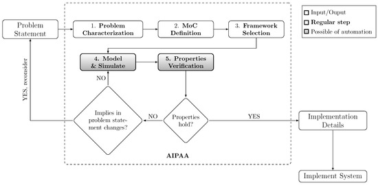
Figure 2.
Analysis and identification of possible automation approaches (AIPAA) applicable to embedded systems design flow. AIPAA needs the “problem statement” as a given input, and aids to produce a model, which is verified and executable, as output. This output can be used as entry point in the implementation domain, e.g., “implementation details” and “implement system”.
3.1. Problem Characterization Step
This first step, problem characterization, aims to conduct an initial analysis on the “problem statement” input aiming the identification of its relevant behaviors and characteristics towards the design of the system.
To facilitate the identification of problem semantics, both the problem procedures and processing must be separated into functions, also defining how they should execute and communicate to each other. These definitions allow for the problem analysis and characterization, which will next support the MoC selection and definition. When applying this step, the following questions must be answered.
- Q1 -
- Does the problem have concurrent, or only sequential, processes?
- Q2 -
- Are the problem communication paths totally or partially ordered?
- Q3 -
- Is the problem a dataflow problem?
- Q4 -
- Are the inputs and processing cyclic?
- Q5 -
- Can a single clock be used to synchronize all the involved processes?
To summarize, the required input for this step is the problem statement describing the problem functionalities, behaviors, inputs and desired outputs. After the application of this step, the expected outputs are the problem separation into functions and their relationship definition, besides a list of well-defined problem characteristics according to the previously stated questions.
3.2. MoC Definition Step
As stated in Section 2.1, models of computation describe only the characteristics that are relevant for a given task. In this sense, it is needed to analyze the problem characterization step outputs aiming the identification of relevant behaviors and functionality that permits its semantics classification into one or more MoCs.
A range of complex applications comprehends behaviors that may not be possible to be modeled using just a single MoC. As a consequence, the model semantics must be split into more than one MoC, generating the concept of heterogeneous systems modeling. In that case, a second phase should be included into this step, defined as MoC division, which classifies each problem characteristic into a MoC that better fits it.
The present paper only addresses the study of a single MoC at a time within a system, that is, using either SY, SDF or SADF MoCs. For this limitation, an analysis on the available MoCs was performed and just three MoCs were selected, based on the criteria that they had to be representative, widely used and should differ on timing abstractions.
As stated in Section 2.1.1, SY is a timed MoC, that is, its signals are totally ordered, and it is based on the perfect synchrony hypothesis. The SDF, on the other hand, is an untimed MoC, that is, its signals are partially ordered, composed by nodes with fixed token rates and it is non-terminating, as described in Section 2.1.2. Finally, the SADF represents a generalization of SDF in which the token rates may vary on each actor fire cycle.
This step’s required input is the list of problem characteristics. After the application of this step, the expected output is the definition of a MoC to be used in the system design flow.
3.3. Framework Selection Step
A support framework is an important tool that aids in the system modeling and simulation step of the design flow. There is a number of facts to be considered when selecting a formal-based framework. The proposed AIPAA method considers the following, based on Reference [8].
- License style: The framework license style must comply with the project requirements. It can vary from open source or freeware to a proprietary and paid license style;
- Included MoCs: The set of available MoCs can drastically differ when comparing frameworks. For example, SDF3 only supports SDF, SADF and CSDF, on the other hand, Simulink, ForSyDe or Ptolemy II supports a range of MoCs. The selected MoC, in Section 3.2, must be part in the framework supported MoC list;
- Capabilities: The frameworks varies on its capabilities, including system simulation and heterogeneous system modeling. In this sense, model simulation figures as an interesting feature for a framework to have;
- Interfaces: Frameworks differ on its modeling and simulation interfaces. It ranges from a script environment to a GUI. The simulation input and output interfaces varies from files, predefined or user inputted and must also be considered;
- Scalability: Towards scalable models, some frameworks are implemented based on programming languages and have interfaces that facilitates the modeling of large or distributed systems;
- Programming language paradigm: Frameworks are based on a wide range of programming languages, leading to a variation on its programming paradigm, for example, imperative or functional. Each paradigm has its own benefits. Functional can lead to a better model scalability and higher abstraction level, on the other hand, imperative paradigm facilitates new MoCs modeling due to inheritance capability.
A research on available frameworks must be performed, submitting them to a posterior analysis considering the previously listed criteria, as a minimum one. Each framework has its own benefits and drawbacks, and as a consequence the framework that best suits the system modeling and simulation varies from one application to another. Horita et al. [8] conducted a research with respect to the framework selection considering a list of predefined parameters and criteria. That work parameters are used in the present research.
This step’s required inputs are the problem characterization and the selected MoC. After the application of this step, the expected output is the definition of the framework to be used for system modeling and simulation.
3.4. Modeling and Simulation Step
The modeling and simulation step next to the properties verification are fundamental steps towards the correct-by-construction design. After the application of these steps, the model correctness can be verified and the system is ready for advancing to the implementation domain.
Based on the problem characterization, the first part of this step is to model the target system, using the previously selected MoC with the aid of the defined support framework.
Aiming the model consistency verification, some frameworks detects model errors during compile time, such as inconsistent types in a communication path and processes missing information, for example, types or number of ports. Besides, a synthetic input data set must be simulated as the last part of this step, aiming the detection of runtime inconsistencies, such as model infinite loops or model acceptance of unwanted inputs types, leading to unexpected behaviors.
In case any model inconsistency is detect, it is necessary to modify and fix the model, recompile and re-simulate it, within an iterative way. After testing boundary conditions and different input types and sizes, resulting in expected outputs and system behavior, the model can be submitted to the next step in the AIPAA context.
This step’s required inputs are problem characterization, besides the selected MoC and framework. After the application of this step, the expected output is the system formally modeled, compiled and simulated aiming its further properties verification.
3.5. Properties Verification Step
After the model consistency is verified, it is necessary to check whether the system model’s properties, with respected to the chosen MoC, hold. This is performed by checking a list of minimum defined system properties.
In this sense, the first part of this step is to identify the minimum or basic properties set that the system must hold. Each MoC comprehends a set of properties that needs to be verified. Besides the in-use MoC specific properties, it is also possible to verify system particular properties in this step. Focusing on the MoCs included in this work scope, the following properties must hold.
- For the SY MoC:
- PSY1
- signals synchronized and totally ordered;
- PSY2
- well-defined absent value for an event; and
- PSY3
- absence of zero-delay feedback, that is, for each loop-back, a delay must be implemented, avoiding algebraic loop. In SY MoC, there are some options to handle loop-backs [31]. The AIPAA method adopts the strategy of forbidden zero-delay loop-backs.
- For the SDF MoC:
- PSDF1
- buffer size determination based on a feasible schedule, that is, the buffers must be in accordance with token rates, so that there is nor data loss neither overflows;
- PSDF2
- system is non-terminating, that is, it cannot have deadlocks;
- PSDF3
- schedulability, that is, it must be possible to extract a valid single-core schedule as a finite sequence of actor firings; and
- PSDF4
- fixed model token rates. As SDF blocks have fixed token rates, the model also will not vary its rates.
- For the SADF MoC [13]:
- PSADF1
- Boundedness: this property is similar to the . The system model production and consumption token rates must be designed in a manner that the number of buffered tokens are bounded;
- PSADF2
- Absence of deadlocks: As SDF, the SADF must be also non-terminating, that is, it must not have deadlocks; and
- PSADF3
- Determinacy: the model performance depends on probabilistic choices that determine the sequence of scenarios selected by each detector. As discussed by Reference [14], in the performance SADF model a detector’s behavior is represented by a Markov chain. On the other hand, in the functional SADF model, representing the detector’s behavior as a Markov chain would violate the tagged signal model definition’s of functional process, since a Markov chain describes more than one behavior, that is, it is non-deterministic. In view of this, the functional model is used in the present work, where the detector’s behavior is dictated by a deterministic finite-state machine.
The last part of this step consists of verifying whether the system holds the minimum listed properties. Some properties are verified by explicit analysis, that is, they are simply MoC intrinsic. For the others, there are different methods for property verification, including mathematical proof, model analysis or test cases application, which is selected based on the property to be verified.
- For the SY MoC:
- VSY1
- Signals are synchronized and totally ordered.This property is MoC intrinsic for SY. As long as the system is modeled following the SY MoC abstraction, this property holds. It is important that the input signals are correctly ordered considering this property, not having unexpected model behaviors. This verification is carried out by explicit model analysis;
- VSY2
- Well-defined absent value for an event.This property is also MoC intrinsic for SY. The framework must handle the absent value for an event towards the maintenance of the perfect synchrony hypothesis; This verification is through explicit model analysis;
- VSY3
- For each loop-back, a delay must be implemented.The verification of this property must be through the model implementation code or interface analysis. First, it is necessary to check whether the model has any loop-back, and in positive case, check the existence of the at least one cycle delay in it. This verification is possible to be automated by using a regular expression checker.
- For the SDF MoC:
- VSDF1
- Buffer size determination based on feasible schedule.The verification of this property can be mathematically demonstrated, as presented by Reference [12]:
- (a)
- Find the model topology matrix ; and
- (b)
- Check if .
- VSDF2
- System is non-terminating.The absence of deadlocks is mathematically proven, as demonstrated by Reference [12]. To verify this property it is necessary to prove the existence of a periodic admissible sequential schedule (PASS), which can be done by performing the following:
- (a)
- Check whether the model holds . If not, the system has no PASS;
- (b)
- Find a positive integer vector q belonging to the null space ;
- (c)
- Create a list L containing all model blocks;
- (d)
- For each block , schedule a feasible one, just once;
- (e)
- If each node has been scheduled times, go to next feasible ; and
- (f)
- If no block in L can be scheduled, the system has a deadlock.
- VSDF3
- Schedulability analysis;For a model to be schedulable, property must hold. Moreover, the model graph must be connected [12]. This must be verified through model analysis.
- VSDF4
- Fixed model token rate.The fixed token rate property is verified by submitting the model to test cases. Different input values and signal sizes must be used to verify the model robustness.
- For the SADF MoC [13]:
- VSADF1
- The boundedness verification considers three aspects:
- (a)
- Boundedness in fixed scenarios case: In case all processes only operate in a fixed scenario, the system behaves as a SDF based model;
- (b)
- The boundedness of control channels: For each kernel k, controlled by a detector d, the inequality must hold for every scenario s in which k is inactive, where represents the duration of d to detect and send the scenario s to kernel k; represents how many cycles the k computation are executed in the scenario s; and is the duration of each k computation cycle; and
- (c)
- The effect of the scenario changes on boundedness: The number of tokens in channels between active processes after an iteration of the SADF model is the same as before. In this context, an iteration is the firing of each process p configured in a scenario s for times.
- VSADF2
- For all kernels’ scenarios combinations, there must have sufficient initial tokens in each cyclic dependency between processes such that every included process can fire a number of times equal to its repetition vector entry. Feedback loops can be considered as a cyclic dependency of a single process; and
- VSADF3
- The functionality non-determinism only occurs between multiple independent concurrent processes. If existing in a model, it leads to satisfying the diamond property. This property states that when two or more independent processes are concurrently enabled, the system functionality is not affected by the order that they are performed. This statement proof is fully described in Reference [13].
This is the last step of the system specification domain. This last AIPAA method step produces a possible entry point for the system implementation domain. For this reason, the system properties’ verification must be checked until the system correctness is proven. The output of this step must be a verified correct simulateable system, which must be also in accordance to the input problem statements.
This step’s required inputs are the MoC minimum properties list and the simulateable system model. After the application of this step, the expected output is a formal-based system executable model with its stated correctness and properties verified.
3.6. Directions to Implementation Details and System Implementation
This section provides some possible directions to the implementation details, as the AIPAA method does not contemplate this domain. System implementation includes complex and extensive procedures and methods that can be considered in future works.
Here, an analysis of systems model and functionalities implementation possibilities is performed, defining a list of implementation details.
- Division of the functionalities implemented in hardware and the ones in software, that is, hardware and software co-design;
- Communication interfaces, methods and protocols;
- Hardware architecture comprehending:
- (a)
- Necessary resources for example, memories, processors, power; and
- (b)
- Necessary units, such as arithmetic logic unit (ALU), floating point unit (FPU), graphics processing unit (GPU), or reconfigurable hardware (FPGA).
- Software architecture comprehending:
- (a)
- Implementation programming language; and
- (b)
- Programming frameworks and tool-chains to be used.
Implementation models can be developed to assist in this analysis [32]. This step represents the base of the system implementation. Related to correct-by-construction methodologies, the definition of implementation details can only proceed when modeling, simulation, and properties checking are already verified.
This step’s required inputs are the problem characterization and a verified system model, besides the hardware, software and communication requirements. After the application of this step, the expected outputs are: system implementation architecture description; hardware platforms to be used; low-level programming language to be used; and software tool-chains to be used.
Based on the listed implementation details, and on the system model from Section 3.4, the system can be implemented using hardware description languages, for example, VHDL or Verilog, and software implementation languages, for example, C, C++ or Assembly.
3.7. Analysis of Possible Automation Approaches
This section introduces two main possibilities identified through the AIPAA method elaboration. The first one is about the properties verification, and the second about automatic code generation.
3.7.1. Proposed Automation to Properties Verification
The properties verification through test cases application is a labor intensive task. For that reason, AIPAA considers the use of a partial automated verification tool towards a faster, more scalable, robust and trustable process.
In this sense Quickcheck can be employed. It is a widely used tool to aid in the process of automatic verification of the system properties generating test cases to evaluate whether the system behaves as expected.
Quickcheck was first presented as a domain-specific language, implemented in Haskell, targeting the test of program properties. It was used as a base for other similar tools having the same purpose.
To accomplish the properties verification, Quickcheck uses predefined verifiable formal system specifications, named properties, as inputs and it automatically generates random values test cases for each one, indicating whether the model holds the desired property.
Considering the MoC properties verification methods (Section 3.5), we present the use of Quickcheck to verify the previously defined property , which is based on the application of test cases. This example assumes the verification of a model containing 2 input signals and 1 output signal. The verification is based on two requirements:
- Req1
- The output signal length divided by its corresponding token rate must be equal to the number of model firing cycles, which is calculated by selecting the smaller division result among the input signal length and its token rates; and
- Req2
- The output signal length should be multiple of its corresponding token rate.
Listing 1 presents the properties to be verified, comprehending the following variables definitions:
- propFixTr21: Fixed token rate property to be verified;
- c1 and c2: Input signals token rates;
- p: Output signal token rate;
- a1 and a2: Quickcheck automatic generated model test cases; and
- actor: The model to be tested.
| Listing 1: Quickcheck usage code example in Haskell/ForSyDe. |
 |
The process propFixTr21 models a function that returns a Boolean value which represents whether the inputted values are according to the described requirements. In this sense, is verified by using native Haskell functions to get the smaller quotient between the input signals length divided by their corresponding token rate. is verified by checking if the remainder of the output signal length divided by its token rate is null.
To illustrate the Quickcheck verification usage, Listing 2 presents a minimal model example based on SDF MoC. In this context, interpolate models a minimal system that interpolates the events of two input signals into one output signal, using the ForSyDe process constructor actor21SDF. The process main uses Quickcheck to verify that the model interpolate holds the property propFixTr21.
| Listing 2: SDF-based system model example code in Hakell/ForSyDe. |
 |
Tests were executed with GHC version 8.6.5, QuickCheck 2.13.2, and ForSyDe 3.4.0.
3.7.2. Automatic Code Generation
The AIPAA output consists on a verified high level abstraction model, in the specification domain. One of the strategies adopted to overcome the abstraction gap in a more robust and scalable manner is a semantic preservation mapping and transformation leading to an automatic code generation using as input the verified formal system model, as the one resulted in the AIPAA.
Automatic code generation is an extensive and complex subject that have been studied and implemented by researchs such as that in References [26,33,34]. In this context, ForSyDe framework includes a deep-embedded DSL, named ForSyDe-Deep [35]. That tool is able to compile and analyze the model, automatically transforming it to be embedded into the hardware target platform.
4. Case Study—Lempel-Ziv-Markov Chain Algorithm
To demonstrate the applicability of AIPAA, we chose the Lempel-Ziv-Markov Chain Algorithm (LZMA). This algorithm is a widely used lossless data compression one, first used in 7z file format [36], and presented as a CPU benchmark in Reference [37]. LZMA intends to generate a compressed file based on the processing of a general data stream input.
LZMA is composed by two compression algorithms. The first one is based on an optimized sliding window encoding (SWE), first presented in LZ77 algorithm [38]. The second algorithm is based on the range encoding (RE) [39]. An additional data filter can be added prior to LZMA default phases (here the word phase is in lieu of step, thus making step reserved for the AIPAA) towards the optimization of the compression rate, such as the delta encoding (DE) algorithm, which encodes each byte of the input stream as its difference from the previous byte. In this case, the first byte is not encoded.
The next sections present the AIPAA method steps application to LZMA, as follows: problem characterization (Section 4.1); MoC definition (Section 4.2); framework selection (Section 4.3); model and simulate (Section 4.4); and properties verification (Section 4.5).
4.1. Problem Characterization Step
This step aims to divide the problem into functions and identify how they behave and communicate with each other. In this sense, the LZMA flowchart is illustrated in Figure 3.
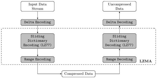
Figure 3.
Lempel-Ziv Markov Chain Algorithm (LZMA) compression and decompression schemes, based on Reference [40].
4.1.1. Sliding Window Encoding (SWE)
The first compression phase is based on LZ77, which searches for a match string of the current look-ahead buffer inside a determined maximum length window already processed. As the bytes are compressed, the look-ahead buffer shifts to the right, together with the search window, thus the name sliding window. For each compression cycle, the LZ77 outputs a tuple containing:
- a distance representing the distance between the current byte and its match in the search window. It is equal to 0 if no match was found and it will be flushed in that case;
- a length representing the match length, that is, how many bytes on the look-ahead buffer were repeated on its match located in the search window. It is equal to 0 if no match was found; and
- a next symbol representing the next symbol in the look-ahead buffer to be processed.
The LZMA sliding window encoding implements additional features towards a higher compression rate, as presented next.
4.1.2. Dictionary Structure
When comparing LZMA to LZ77, the sliding window encoding supports larger dictionaries, which demands an optimized search structure targeting a faster algorithm. The LZMA implements two structure options that can be configured prior to the compression start, the hash-chain and binary trees [41]. Both of them are based on arrays of dynamically allocated lists, called hash-arrays. Each index of the array corresponds to a number N of bytes that are hashed from the input stream at each compression cycle.
The hash-chain array comprehends an array of linked lists. The nodes list contains the positions of the corresponding N hashed bytes of that array index in the input stream. The linked list can be long, and searching for the best match would result in a slow algorithm. For that reason, LZMA only checks for matches considering the 24 most recent positions.
In the binary tree, the nodes of its structure contains the same information as the hash-chain, with an optimized search structure, the binary tree. The most recent occurrences are closer to the tree root. Besides, the tree adopts the lexicographic ordering algorithm.
Without loss of generality, the present case study adopts the hash-chain array dictionary. When compared to the binary tree, the dictionary structure is simpler and the search algorithm is faster, since it limits the number of previously processed hash bytes analysis when finding a match.
Besides the dictionary structure, LZMA also employs an array containing the 4 last used match distances. If the distance of a match is equal to one of this array entries, the 2-bit array index is used to encode this variable [41].
4.1.3. Output Format
The LZMA sliding window encoding comprehends a range of compressed packages possibilities that depends on the identified matches. Table 1 shows the output alternatives, presenting a brief description of each tuple.

Table 1.
Sliding window encoding output packages, based on source code [36]. The symbol ⊕ represents concatenation of binary values.
4.1.4. Range Encoding (RE)
The range encoding (RE) algorithm was first presented by Martin [39]. It consists of a context-based compression algorithm in which the compressed range in each iteration is estimated based on probabilistic algorithms, and it can form a set of predefined types of packages depending on the input range size.
The LZMA range encoding performs a bit-wise compression of a sliding window tuple output at each fire cycle, outputting encoded bytes to the final output stream. It can be configured to update its bit probability at each process cycle, or to use fixed compression probability.
Based on the described LZMA functions and their relationship, the analysis of the problem behavior lies on the questions in Section 3.1, which are answered as follows:
- Q1 -
- The problem has no concurrent processes, that is, the functions are sequentially executed;
- Q2 -
- The problem communication paths are partially ordered, that is, it is not possible to determine the sequence of tokens considering different data paths;
- Q3 -
- the model does not have any deadlock and will be finished only when there is no data in the input stream;
- Q4 -
- the processing of the input streams are cyclic and non-terminating; and
- Q5 -
- The functions cannot be synchronized by a clock, they depend on the data tokens outputted by other functions.
4.2. MoC Definition Step
The LZMA compression comprehends the processing of an input stream, through defined phases, resulting in a compressed output stream. This behavior is classified as untimed and concurrent, which is according to the theory and semantics of the dataflow MoC family.
A first simplified LZMA model was introduced by the author of the present research in Reference [42] using the SDF MoC. That simplified LZMA modeling considered a set of assumptions to be valid. It was assumed that predefined fixed token rates for each actor port applies. Although it models the system process flow, it does not fully address the dynamic behavior of each compression phase, that is, both the sliding window and the range encoding. In this sense, the dynamic LZMA behavior can be better modeled based on the scenario-aware dataflow (SADF) MoC.
4.3. Framework Selection Step
Framework ForSyDe was used for the LZMA modeling and simulation, following the same criteria used in Reference [8]. For the sake of convenience, the points from Reference [8] are listed next.
- License style: the present research work focus is on open source tools;
- Included MoCs: the framework must include the selected MoC, that is, SADF;
- Capabilities: the proposed design includes both modeling and simulation;
- Interfaces: this case study accepts inputs and output from an user interface or from files;
- Scalability: this case study targets model high scalability. In this sense, a text-based coding interface is better than a GUI;
- Programming language paradigm: towards a higher level of abstraction, Haskell, a pure functional programming language, was selected as the framework base language.
A functional model for the scenario-aware dataflow (SADF) model of computation (MoC), as well as a set of abstract operations for simulating it was introduced in Reference [14]. That MoC library is implemented on top of ForSyDe, and it is used in the present research to model and simulate the LZMA according to the SADF semantics.
4.4. Modeling and Simulation Step
The case study is formal modeled in this step, using the previously selected MoC and framework, that is, SADF and ForSyDe. The model consistency is verified through a simulation aiming a correct-by-construction design, as described in Section 3.4. This case study considers only the LZMA compression phase. Assuming that the decompression phase comprehends similar processes, it will not be modeled here.
4.4.1. SADF LZMA Model Description
The LZMA compression takes an input data stream, processes it through two compression phases and produces a compressed data output stream, as previously illustrated in Figure 3.
When modeling LZMA using SADF MoC library from ForSyDe, the data streams are represented by signals, and the processing components by kernels. Besides, a detector is used to control the LZMA dynamic behavior. Figure 4 illustrates the LZMA high level modeling dataflow graph based on SADF MoC.
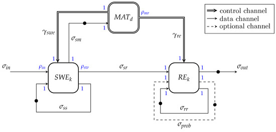
Figure 4.
LZMA high level modeling dataflow graph based on SADF model of computation (MoC). Initial tokens are represented by •.
Kernels, detector, signal paths, token rates and types in the model (Figure 4) are defined as follows:
- is the match detector, which controls the scenarios from both kernels, and . In this sense, comprehends two scenarios, that is, and , as described in Table 2;
Table 2. output control channels token rates and scenarios discrimination.
- -
- The input signal transmits the current status of ;
- -
- The scenarios, , are outputted to the signal , according to Table 3;
Table 3. Scenarios and token rates discrimination.
- -
- Although contains a single scenario, , the control channel is needed for detector to reach a system feasible schedule. To model this behavior, its output token rate can vary from 0 to 1;
- is the sliding window encoding kernel, which compresses the input stream by outputting processed tokens. Without loosing system main behavior and properties, the present modeling adapts the dictionary structure to a sliding window method based on the original LZ77 algorithm, aiming a simple model however preserving its behavior and properties.
- -
- The is an input signal, representing a stream to be compressed. Our model considers the input stream to be always finished with the NULL character;
- -
- The consumption token rate depends on the current scenario, as described in Table 3. It can vary from 0 to 1 . Each represents a character from the input stream;
- -
- The feedback signal carries tuples . In this context, represents the window dictionary, represents a package which is being processed, and models the latest four used distances vector;
- -
- is a signal which carries the produced tokens to ;
- -
- The production token rate can vary depending on the kernel scenario, from 0 to 1 , as described in Table 3. The possible formats are described in Table 4 and Table 5. The original LZMA encodes the variable , contained in format , with different number of bits and contents depending on the match distance value. Our model simplifies the variable encoding, assuming it to be an integer composed by 8 bits;
Table 4. possible token formats.
Table 5. l variable possible sizes.
- -
- The control channel, signal , carries tokens comprehending the possible scenarios ; and
- -
- The signal carries Boolean values that are either , if a package was processed and is ready to be outputted, or otherwise.
- is the range encoding kernel, which performs a bit-wise compression of packages, outputting encrypted bytes to LZMA output stream. Although its token rates are all constants, its fire cycles are controlled by the detector ;
- -
- The input port, connected to the signal , has a fixed consumption token rate equals to ;
- -
- The input control port, connected to the signal , has a fixed consumption token rate of 1;
- -
- The output signal carries the LZMA output stream, composed by encrypted bytes produced by . The fixed output token rate is , consisting on a signal of bytes;
- -
- Signal carries tuples that contains the relevant variables for the range encoding, that is, . In this context, represents the considered range when encoding the next bit. represents the lower limit of the considered range for the next bit encoding. represents a processed value to be outputted to in the next range encoder token production;
- -
- Signal (dashed line in Figure 4) represents the bit probabilities updated at each compression cycle, in case the variable probability is configured. Although the fixed probability configuration has a reduction in the compression rate performance taking into account some cases where the bits patterns are often repeated, there is no loss of generality when considering fixed bit probabilities. In this sense, the present work assumes the range encoder configured to use fixed probability encoding; and
- -
- The initial token in the signal is the compressed file header, which includes LZMA configuration, dictionary size and decompressed file size.
Based on the described definitions, this modeling considers two system scenarios, which are controlled by the detector .
4.4.2. LZMA Modeling with ForSyDe SADF MoC
ForSyDe is used to system modeling based on the model description previously stated and illustrated in the dataflow graph from Figure 4. The model main definitions and processes (that is, kernel, detector, actor) signatures are presented in Listing 3, using the process constructors from the ForSyDe SADF MoC library. In this context, the following concepts are used:
- SWEData represents de kernel output token type, which can be derived to all the package types;
- SWEkScenario and REkScenario models the kernels and scenarios, respectively;
- RangeVars models the tokens contained in the feedback signal , which comprehends the current encoding , its value and the , representing a stored byte to be outputted when the next output token is produced;
- matD models the detector using the ForSyDe process constructor detector12SADF, with one input port and two control output ports;
- sweK models kernel using the process constructor kernel23SADF, indicating it contains two data input ports and three data output ports; and
- rek represents the range encoder kernel , modeled using the process constructor kernel22SADF, indicating it contains two data input ports and two data output ports;
| Listing 3: LZMA model signatures and definitions in Haskell/ForSyDe. |
 |
Each actor is then presented in separate listings. The LZMA detector model main functions and definitions are presented in Listing 4, with the following definitions:
- FDscenario represents the detector scenario, comprehending the output token rates of the control channels ports and the sent kernels scenarios. FDstate models the detector state, based on the kernel boolean output through ; and
- matStateTran represents the detector function to select the scenarios based on a Boolean input, and matStateOut outputs the and scenarios.
| Listing 4: LZMA detector model functions in Haskell/ForSyDe. |
 |
Listing 5 introduces the main functions used to model the LZMA sliding window kernel , with the following definitions:
- sweSearch and sweFlush model the functions executed by sweK depending on its scenario, where:
- -
- sweSearch represents the scenario in which consumes a character from input signal when searching for a match; and
- -
- sweFlush models the output of a found package to signal .
| Listing 5: LZMA sliding window kernel main functions in Haskell/ForSyDe. |
 |
The range encoder main functions and definitions are presented in Listing 6 with the following definitions:
- encBit models the bit-wise processing of the tokens, updating the RangeVars variables;
- normRange models the normalization procedure, executed when the range reaches its lower limit and needs to be re-scaled, producing one byte that will be outputted to the signal, temporarily stored in Cache;
- normFinalRange and finalBytes models the final normalization cycles executed by ;
- rekStdBy models the standby state of kernel , while waiting for a token; and
- rekRead models the function to read a token and encrypt it to .
| Listing 6: LZMA range encoding kernel main functions in Haskell/ForSyDe. |
 |
Finally, the complete process network is shown in Listing 7. The process lzmaCompressPn models the LZMA compression, connecting the sweK output to the reK input. The compressed stream is modeled as sig_out and the input stream as sig_in. In addition, the sliding window encoder process network is also presented as swePn to illustrate and test this compression step separately.
| Listing 7: LZMA compression process network in Haskell/ForSyDe. |
 |
4.4.3. Model Simulation
Towards the verification of system consistency and behavior in accordance to the expected original LZMA results, some input stream examples are used to test the LZMA model. This step is based on the GHCi usage.
Listing 8 introduces the defined processes to simulate the model. sweOutTest models the sliding window output, and lzmaOutTest the LZMA compression output. For a printable character set, lzmaOutTest in outputted as Integer values, based on the ASCII table.
| Listing 8: LZMA compression test processes. |
 |
The first example consists on a sequence of five characters, non repeated. Its simulation was successfully accomplished, as presented in Listing 9. The model behaves as expected. The outputs the correct packages, that is, literals, as it has no repetitions. The LZMA outputs the expected stream of encoded bytes, composed by an initial header followed by a sequence of byte lists, grouped by the output of each cycle.
| Listing 9: LZMA compression input example #1. |
 |
The second example comprehends the inclusion of a package of a found match. Listing 10 presents the simulation results. The model also behaves as expected in this example, identifying the match in the previous buffer and successfully encoding all the packages.
| Listing 10: LZMA compression input example #2. |
 |
In the third example, the empty input boundary case is tested, as presented in Listing 11. The outputs an empty package to , which in turn, just outputs the header, without any data to be compressed, as expected.
| Listing 11: LZMA compression input example #3. |
 |
As the model compiles with no errors and behaves as expected in all the presented simulations, its consistency verification is finished.
4.5. Properties Verification Step
This step aims to check whether the system model holds the required properties, with respect to the in-use MoC. In this sense, this section introduces the LZMA model verification based on the SADF MoC properties, presented in the Section 3.5.
- VSADF1
- BoundednessProperty verification—The three verification aspects are considered for the presented LZMA model:
- (a)
- The first aspect is used for verification of models where all the processes comprehend a single scenario. In the LZMA case, the kernel and detector do not operate in a single scenario, as described in Section 4.4.1. In this sense, this aspect is not applicable;
- (b)
- The LZMA kernel becomes inactive during the detector scenario . In this model, the range encoder fires a single time for each scenario selection (). For the model to be bounded, the duration has to be smaller than the duration between two scenarios detection by ;
- (c)
- The third aspect must be analyzed focusing on kernel and detector , as these are the only processes with multiple scenarios. The interface between these processes consists on a cyclic dependency with fixed and equal token rates, not representing an unboundedness risk. Regarding the boundedness of signal , the production token rate from output port is controlled by , and the consumption token rate from is always one. In scenario , will not produce any tokens in , and in scenario , will produce one token that will be promptly consumed by in the same iteration. In this context, the third boundedness aspect will always hold, as controls the system schedule, so that will not produce another token before consumes the last one.
- VSADF2
- Absence of deadlocksProperty verification—Analyzing the LZMA model, the included cyclic dependency are the feedback signals , and , in addition to the and processes cycle. Initial tokens were added to each of these cycles, satisfying the necessary consumption token rates. As a consequence, it is verified that the LZMA system holds this property.
- VSADF3
- DeterminacyProperty verification—The LZMA does not comprehend multiple independent concurrent processes, as the depends on and vice-versa. Besides, also depends on . As a consequence, the system holds the determinacy property.
In addition to the introduced properties verification arguments and , Table 6 presents a feasible LZMA static sequential schedule, representing a possible sequence of determined running processes, starting with an initial token in signal , and without any deadlock. The reads the initial token S, and sets the system to scenario. generates the detector input at each fire cycle. The schedule finishes when input stream is empty.
Table 6.
A feasible LZMA system static sequential schedule. Token where S = Search and F = Flush.
4.6. Implementation Details and Implement System
The implementation domain is not part in AIPAA scope. Nevertheless, different programming languages, implementation architectures and platforms have been used to implement the LZMA in other related works. But, no implementation was found based on a functional programming language, such as Haskell.
The first LZMA implementation was presented in the 7zip open source application, able to be executed using different platforms, including a range of compression algorithms, and having LZMA as default [36,41]. Another similar application is presented in XZ Utils, having less languages and configuration options [43]. Besides the mentioned applications, hardware description languages (HDL) implementations for FPGA are also available in the literature [40,44]. A benchmark comparing different implementation architectures and platforms was presented by SPEC.
5. Results and Discussion
AIPAA includes two steps aiming the formal-based modeling: the system model functional correctness verification and the consistency. The referred steps are model and simulate and model properties verification, described in Section 3.4, Section 3.5, respectively.
A comprehensive case study was based on Reference [42] published by the authors of this work. That paper modeled the LZMA compression using the ForSyDe SDF MoC library, but not representing part of the system dynamic behavior. The present paper modeled the same algorithm, but now using the ForSyDe SADF MoC library, as described in Section 4.4 and illustrated in Figure 4. The present case study addressed the compression procedure inherent dynamism. Besides, AIPAA method was used to prove the model holds SADF MoC properties (Section 4.5).
The AIPAA method comprehends the specification domain, which outputs a verified high level abstraction executable model.
The implementation domain consists of an extensive subject and, although it is not included in AIPAA, Section 3.6 presents directives on how to overcome the abstraction gap and implement a system based on a verified model. Besides, for case study, implementation related works were cited as a reference to guide possible future researches.
5.1. Analysis Identifying Steps to be Automated
AIPAA includes well-defined design steps on a formal base, making the automation approaches identification feasible and possible to be systematically analyzed.
As a result, this research introduced in Section 3.7, as possible of automation steps the properties verification and the automatic code generation based on a formal and verified model, as follows.
5.1.1. Properties Verification with the Tool Quickcheck
AIPAA also includes a step comprehending the system model properties verification, as described in Section 3.5. Its main purpose is to prove that the model holds the properties of the selected MoCs and possibly a set of system specific properties. In this sense, a range of methods can be applied to verify if the system holds each property, for example, mathematical prove and model analysis.
A widely used method for properties verification is the system submission to a range of test cases, which can be a labor intensive task. Besides, for a robust verification, different tests must be elaborated aiming the detection of different fail cases.
The present research identifies the automation of this verification method as a possibility. In this sense, Section 3.7.1 presents Quickcheck as an alternative for automatic test cases generation and system property verification. A minimal model example based on SDF MoC was presented, using Quickcheck for verification whether the system holds the property , introduced in Section 3.5, as an example of its applicability.
5.1.2. Automatic Code Generation
Although the implementation domain is not included in AIPAA, this research recognizes the abstraction gap between the formal-based model outputted by the introduced method and the implemented system and the difficulties to overcome it. In this sense, this research proposes, as an embedded design automation approach, the automatic low level code generation based on a verified formal-based model. This represents an extensive work that have been studied in related works and can be deeper explored as future works, as mentioned in Section 3.7.2.
6. Conclusions
We presented a method to aid in the identification of possible automation approaches within design flows based on formal models of computation. The method aims to assist in a low-level implementation of automatic code generation and also a trustable, robust and scalable embedded systems design flow.
Our method for analysis and identification of possible automation approaches (AIPAA) includes five basic steps:
- problem characterization—to identify the relevant behaviors and characteristics of the target problem, defining intermediate functions that can represent the system processes and their relationships;
- MoC definition—based on problem characteristics, select a MoC to be used in the system design flow;
- framework selection—to define the formal-based framework for system modeling and simulation;
- model & simulate—to model the specified system, simulating it to verify its consistency;
- properties verification—to verify that the system model holds the defined MoC properties.
To develop a deeper analysis method, a review of the formal-based design flow concepts was performed, including embedded systems, modeling frameworks, MoCs topology and programming paradigms.
To demonstrate the AIPAA application, a case study was presented, taking the Lempel-Ziv Markov Chain Algorithm (LZMA).
The AIPAA application results were discussed, identifying the properties verification and automatic code generation as possible embedded systems design flows’ automation approaches. In this context, the model’s properties verification and low abstraction level code generation were pointed as steps that can be automated. The authors of this work believe that the automation of formal-based design methods is an important alternative to increase the robustness and scalability of CPS and embedded systems development.
The possible automation approaches identified by AIPAA application in the case study, that is, properties verification and low level source code generation, are intended to be implemented as future works.
Author Contributions
Conceptualization, A.Y.H. and D.S.L.; methodology, A.Y.H. and D.S.L.; software, A.Y.H. and R.B.; validation, A.Y.H. and R.B.; formal analysis, A.Y.H.; investigation, A.Y.H.; resources, A.Y.H.; writing—original draft preparation, A.Y.H.; writing—review and editing, A.Y.H., D.S.L. and R.B.; supervision, D.S.L. All authors have read and agreed to the published version of the manuscript.
Funding
This research received no external funding.
Acknowledgments
The authors thank UNICAMP for awarding studies opportunity that supported this research work.
Conflicts of Interest
The authors declare no conflict of interest.
References
- Lee, E.A. CPS foundations. In Design Automation Conference; ACM Press: New York, NY, USA, 2010. [Google Scholar] [CrossRef]
- Edwards, S.; Lavagno, L.; Lee, E.; Sangiovanni-Vincentelli, A. Design of embedded systems: Formal models, validation, and synthesis. Proc. IEEE 1997, 85, 366–390. [Google Scholar] [CrossRef]
- Jantsch, A.; Sander, I. Models of computation and languages for embedded system design. IEE Proc. Comput. Digit. Tech. 2005, 152, 114. [Google Scholar] [CrossRef]
- Ptolemaeus, C. (Ed.) System Design, Modeling, and Simulation Using Ptolemy II. Available online: https://ptolemy.berkeley.edu/books/Systems/chapters/HeterogeneousModeling.pdf (accessed on 21 February 2020).
- Sander, I.; Jantsch, A.; Attarzadeh-Niaki, S.H. ForSyDe: System Design Using a Functional Language and Models of Computation. In Handbook of Hardware/Software Codesign; Springer: Amsterdam, The Netherlands, 2016; pp. 1–42. [Google Scholar] [CrossRef]
- Stuijk, S.; Geilen, M.; Basten, T. SDF3: SDF For Free. In Proceedings of the Sixth International Conference on Application of Concurrency to System Design (ACSD’06), Turku, Finland, 28–30 June 2006; pp. 276–278. [Google Scholar] [CrossRef]
- MathWorks. Simulink Documentation. 2019. Available online: https://www.mathworks.com/help/simulink/index.html (accessed on 21 February 2020).
- Horita, A.Y.; Bonna, R.; Loubach, D.S. Analysis and Comparison of Frameworks Supporting Formal System Development based on Models of Computation. In 16th International Conference on Information Technology-New Generations (ITNG 2019); Latifi, S., Ed.; Springer International Publishing: Cham, Switzerland, 2019; pp. 161–167. [Google Scholar]
- Jantsch, A. Models of Embedded Computation. In Embedded Systems Handbook; Chapter Models of Embedded Computation; CRC Press: Boca Raton, FL, USA, 2005. [Google Scholar]
- Lee, E.; Sangiovanni-Vincentelli, A. A framework for comparing models of computation. IEEE Trans. Comput.-Aided Des. Integr. Circuits Syst. 1998, 17, 1217–1229. [Google Scholar] [CrossRef]
- Benveniste, A.; Berry, G. The synchronous approach to reactive and real-time systems. Proc. IEEE 1991, 79, 1270–1282. [Google Scholar] [CrossRef]
- Lee, E.; Messerschmitt, D. Synchronous data flow. Proc. IEEE 1987, 75, 1235–1245. [Google Scholar] [CrossRef]
- Theelen, B.D.; Geilen, M.C.W.; Basten, T.; Voeten, J.P.M.; Gheorghita, S.V.; Stuijk, S. A scenario-aware data flow model for combined long-run average and worst-case performance analysis. In Proceedings of the MEMOCODE ’06 Fourth ACM and IEEE International Conference on Formal Methods and Models for Co-Design, Napa, CA, USA, 27–30 July 2006; pp. 185–194. [Google Scholar] [CrossRef]
- Bonna, R.; Loubach, D.S.; Ungureanu, G.; Sander, I. Modeling and Simulation of Dynamic Applications using Scenario-Aware Dataflow. ACM Trans. Des. Autom. Electron. Syst. 2019, 24, 5. [Google Scholar] [CrossRef]
- Association, T.M. Modelica Website. 2019. Available online: https://www.modelica.org/ (accessed on 21 February 2020).
- Open Source Modelica Consortium (OSMC). OpenModelica Website. 2019. Available online: https://openmodelica.org/ (accessed on 21 February 2020).
- Mathaikutty, D.; Patel, H.; Shukla, S.; Jantsch, A. EWD: A Metamodeling Driven Customizable multi-MoC System Modeling Framework. ACM Trans. Des. Autom. Electron. Syst. 2008, 12, 33:1–33:43. [Google Scholar] [CrossRef]
- Herrera, F.; Villar, E. A framework for heterogeneous specification and design of electronic embedded systems in SystemC. ACM Trans. Des. Autom. Electron. Syst. 2007, 12, 22. [Google Scholar] [CrossRef]
- Sander, I.; Jantsch, A. Formal system design based on the synchrony hypothesis, functional models, and skeletons. In Proceedings of the IEEE, Twelfth International Conference on VLSI Design, (Cat. No. PR00013), Goa, India, 7–10 January 1999. [Google Scholar] [CrossRef]
- University of California B.o. ICyPhy Home Page. 2018. Available online: https://ptolemy.berkeley.edu/projects/icyphy/ (accessed on 21 February 2020).
- Jantsch, A. Modeling Embedded Systems and SoC’s; Morgan Kaufmann: San Francisco, CA, USA, 2003. [Google Scholar]
- ForSyDe Group, K. ForSyDe Hackage Page. 2019. Available online: https://forsyde.github.io/tools.html (accessed on 30 April 2018).
- Turner, D.A. Some History of Functional Programming Languages. In Trends in Functional Programming; Loidl, H.W., Peña, R., Eds.; Springer Berlin Heidelberg: Berlin/Heidelberg, Germany, 2013; pp. 1–20. [Google Scholar]
- Haskell. The Haskell Purely Functional Programming Language Home Page. 2018. Available online: https://www.haskell.org (accessed on 21 February 2020).
- Scott, M.L. Programming Language Pragmatics, 3rd ed.; Morgan Kaufmann Publishers Inc.: San Francisco, CA, USA, 2009. [Google Scholar]
- MathWorks. Simulink Embedded Coder Website. 2019. Available online: https://www.mathworks.com/products/embedded-coder.html (accessed on 21 February 2020).
- Krizan, J.; Ertl, L.; Bradac, M.; Jasansky, M.; Andreev, A. Automatic code generation from Matlab/Simulink for critical applications. In Proceedings of the 2014 IEEE 27th Canadian Conference on Electrical and Computer Engineering (CCECE), Toronto, ON, Canada, 4–7 May 2014; pp. 1–6. [Google Scholar] [CrossRef]
- Pike, L.; Wegmann, N.; Niller, S.; Goodloe, A. Copilot: Monitoring embedded systems. Innov. Syst. Softw. Eng. 2013, 9. [Google Scholar] [CrossRef]
- Rash, J.L.; Hinchey, M.G.; Rouff, C.A.; Gračanin, D.; Erickson, J. A requirements-based programming approach to developing a NASA autonomous ground control system. Artif. Intell. Rev. 2006, 25, 285–297. [Google Scholar] [CrossRef]
- Seshia, S.A.; Hu, S.; Li, W.; Zhu, Q. Design Automation of Cyber-Physical Systems: Challenges, Advances, and Opportunities. IEEE Trans. Comput.-Aided Des. Integr. Circuits Syst. 2017, 36, 1421–1434. [Google Scholar] [CrossRef]
- Sander, I. System Modeling and Design Refinement in ForSyDe. Ph.D. Thesis, Royal Institute of Technology KTH, Stockholm, Sweden, 2003. [Google Scholar]
- Loubach, D.S. A runtime reconfiguration design targeting avionics systems. In Proceedings of the 2016 IEEE/AIAA 35th Digital Avionics Systems Conference (DASC), Sacramento, CA, USA, 25–29 September 2016; pp. 1–8. [Google Scholar] [CrossRef]
- Bourke, T.; Colaço, J.L.; Pagano, B.; Pasteur, C.; Pouzet, M. A Synchronous-Based Code Generator for Explicit Hybrid Systems Languages. In Lecture Notes in Computer Science; Springer: Berlin/Heidelberg, Germany, 2015; pp. 69–88. [Google Scholar] [CrossRef]
- Grabmüeller, M.; Kleeblatt, D. Harpy. In Proceedings of the ACM SIGPLAN Workshop on Haskell Workshop-Haskell 07; ACM Press: New York, NY, USA, 2007. [Google Scholar] [CrossRef]
- Acosta, A. ForSyDe Tutorial Website. 2008. Available online: https://hackage.haskell.org/package/ForSyDe-3.1/src/doc/www/files/tutorial/tutorial.html (accessed on 21 February 2020).
- Pavlov, I. 7z Format. 2019. Available online: http://www.7-zip.org/7z.html (accessed on 21 February 2020).
- Standard Performance Evaluation Corporation (SPEC). 657.xz_s SPEC CPU 2017 Benchmark Description. 2019. Available online: http:/www.spec.org/cpu2017/Docs/benchmarks/657.xz_s.html (accessed on 21 February 2020).
- Ziv, J.; Lempel, A. A universal algorithm for sequential data compression. IEEE Trans. Inf. Theory 1977, 23, 337–343. [Google Scholar] [CrossRef]
- Martin, G.N. Range Encoding: An Algorithm for Removing Redundancy from a Digitized Message. Available online: https://pdfs.semanticscholar.org/3a46/423f866d53d4e0328faf365c4c9101f82577.pdf?_ga=2.221534352.907706746.1582276987-231942018.1567670099 (accessed on 21 February 2020).
- Leavline, E.J. Hardware Implementation of LZMA Data Compression Algorithm. Int. J. Appl. Inf. Syst. (IJAIS) 2013, 5, 51–56. [Google Scholar]
- Salomon, D. Data Compression: The Complete Reference; with contributions by Giovanni Motta and David Bryant; Springer: Berlin, Germany, 2007; p. 1092. [Google Scholar]
- Horita, A.Y.; Bonna, R.; Loubach, D.S. Lempel-Ziv-Markov Chain Algorithm Modeling using Models of Computation and ForSyDe. In Proceedings of the Aerospace technology Congress 2019 (FT2019), Stockholm, Sweden, 8–9 October 2019. [Google Scholar]
- Collin, L. XZ Utils. 2019. Available online: https://www.tukaani.org/xz/ (accessed on 21 February 2020).
- Zhao, X.; Li, B. Implementation of the LZMA compression algorithm on FPGA. In Proceedings of the 2017 International Conference on Electron Devices and Solid-State Circuits (EDSSC), Hsinchu, Taiwan, 18–20 October 2017; pp. 1–2. [Google Scholar] [CrossRef]
© 2020 by the authors. Licensee MDPI, Basel, Switzerland. This article is an open access article distributed under the terms and conditions of the Creative Commons Attribution (CC BY) license (http://creativecommons.org/licenses/by/4.0/).