Article

GPRS Sensor Node Battery Life Span Prediction Based on Received Signal Quality: Experimental Study

1
African Center of Excellence in Internet of Things, College Of Science and Technology, University of Rwanda, Kigali 4285, Rwanda
2
Abdus Salam International Centre for Theoretical Physics (ICTP), Strada Costiera, 11, I-34151 Trieste, Italy
3
Department of Physics, University of Malawi, P.O. Box 280, Zomba, Malawi
4
Department of Computer Engineering, Copperbelt University, P.O. Box 21692, Kitwe, Zambia
5
Department of Information Technology, School of Computing, SRM Institute of Science and Technology, Chennai 603203, India
*
Author to whom correspondence should be addressed.
Information 2020, 11(11), 524; https://doi.org/10.3390/info11110524
Submission received: 25 September 2020 / Revised: 25 October 2020 / Accepted: 26 October 2020 / Published: 11 November 2020
(This article belongs to the Special Issue Wireless IoT Network Protocols)

Abstract

:
Nowadays with the evolution of Internet of Things (IoT), building a network of sensors for measuring data from remote locations requires a good plan considering a lot of parameters including power consumption. A Lot of communication technologies such as WIFI, Bluetooth, Zigbee, Lora, Sigfox, and GSM/GPRS are being used based on the application and this application will have some requirements such as communication range, power consumption, and detail about data to be transmitted. In some places, especially the hilly area like Rwanda and where GSM connectivity is already covered, GSM/GPRS may be the best choice for IoT applications. Energy consumption is a big challenge in sensor nodes which are specially supplied by batteries as the lifetime of the node and network depends on the state of charge of the battery. In this paper, we are focusing on static sensor nodes communicating using the GPRS protocol. We acquired current consumption for the sensor node in different locations with their corresponding received signal quality and we tried to experimentally find a mathematical data-driven model for estimating the GSM/GPRS sensor node battery lifetime using the received signal strength indicator (RSSI). This research outcome will help to predict GPRS sensor node life, replacement intervals, and dynamic handover which will in turn provide uninterrupted data service. This model can be deployed in various remote WSN and IoT based applications like forests, volcano, etc. Our research has shown convincing results like when there is a reduction of −30 dBm in RSSI, the current consumption of the radio unit of the node will double.

1. Introduction

The internet of things (IoT) is expected to transform almost countless industries including retail, manufacturing, energy, healthcare, education, and transportation. Before building your first IoT network, you have to consider some parameters like the availability of unlicensed frequency and degree of occupancy, availability of service provider, the number of devices to be deployed, number and frequency of message, minimum latency, maximum payload, battery duration, etc. These parameters are the ones to determine the cost for your network [1]. However, the chosen technology will have a big impact on the whole network cost. In Rwanda, especially in Kigali, building a sensor network for IoT applications that can work on technologies like Lora and Sigfox may imply a higher initial cost because of the geographical situation of the country; this will require a lot of base stations or gateways. The GSM cellular network covers 96.4% of the country [2]. This means that any application based on cellular communication will not cost a lot as the network infrastructure is already in place. In this paper, we are trying to work on GSM/GPRS sensor node which can be used to build a WSN or IoT application in Rwanda, without spending a lot of money and we will try to mathematically demonstrate the impact of received signal strength indicator (RSSI) on the power consumption of GPRS Sensor node which will finally help in estimating battery life span. There is a challenge for sensor nodes supplied by batteries, due to power consumption which will even determine the lifetime of the node and the network in general. The battery energy is influenced by the operating temperature and the total current consumption of the node [3,4]; apart from this, sampling rate, signal strengths, and network topology affect the battery life of sensor node [5,6], while other researchers found that factors like energy harvesting, energy transfer, energy conservation, and efficient routing techniques can help in prolongation of the lifetime of a sensor node [7,8]. The big percentage of power consumed by the sensor node is taken by transceiver or radio section: receiving part 26.67% and the transmitting part 33.3 % [8]. In cellular communication, a mobile phone is communicating with the nearest base transceiver station (BTS); the output power from a mobile phone will depend on received signal strength information (RSSI) at that particular location. If the distance between the mobile phone and the nearest BTS is high, the mobile phone will use a lot of power trying to amplify for getting better reception for that weak signal [9]. On the other hand, if the distance is short the phone will output low power as the signal is strong enough which makes the communication easy. The scenario which is happening is almost the same as in human being communication; when someone with whom you are communicating is far away, you will have to use a lot of energy for the communication to be effective and if you are near each other, low energy is used for communication. The amplification of the received signal does not require any extra battery power but, in the situation when the received signal is weak, the mobile phone will try to boost its transmitter power expecting that it will increase the quality of the signal from the base stationl [9]. Then the increase in transmitter power will drain the battery more than in a location with good signal quality. A GPRS sensor node is like a mobile phone, it will transmit data through its nearest BTS as it is shown in Figure 1. In this paper, we are trying to show that when our sensor node has poor signal quality it will try to increase its transmitter power for better reception; this will consume a lot of energy from the battery. In the end, we will demonstrate the relationship between the power consumption and the signal quality (RSSI) at a particular location and this relationship will bring us to mathematically estimate the battery life of a GPRS sensor in that region. In this paper, we have tried to record the current consumption of our GPRS sensor node for six different locations with different received signal strength information (RSSI) levels. For each location, we have recorded: a. Reference current which is the consumed current when the GSM/GPRS module is switched off. b. GSM current which is current when the module is switched ON and connected to the network. And, c. GPRS current which is current when the module is transmitting data to a remote server and the RSSI value. Each of the above parameters has been recorded for 24 h. The received strength signal indicator (RSSI) is an important parameter which shows the quality of the signal which is being received by a receiver; this parameter depends mainly on the power which has been transmitted, the distance between the transmitter and receiver, and the medium between the transmitter and receiver [10]. A lot of research has been conducted about the localization of the receiving sensor node using RSSI and some research demonstrated that there is an impact of RSSI on the drainage of the battery. In this paper, we are trying to find the mathematical model which shows the effect of the RSSI on the power consumption of a receiving GPRS based sensor node and from here we will also estimate the sensor node lifetime.
In our paper, we did our experiment with an IoT application that we can call “Remote temperature monitor (RTM)” which is sending temperature from five different locations to a remote server and at a rate of 20 s; we then try to see how this application will consume current in different locations remembering that each location will be defined by its RSSI. Then we used results from our measurement to derive a mathematical model that links the received strength signal information and the sensor node lifetime. With this, it will be possible to quantitatively understand how poor signal quality will reduce the lifetime of a sensor node, especially a GSM-based node. Basically, we are considering our sensor node as a mobile phone with only one application of sending data to the cloud. This can be applied both indoor as well as outdoor. During our modeling, we are supposing that:
  • Our sensor node is not moving,
  • The rate with which the sensor node is transmitting data is fixed,
  • All sensors in the network are not moving, and
  • The sensor node is dead if and only if the battery voltage drops to 70% of its full charged voltage [11,12].
Our contribution is to develop a data-driven mathematical model that shows the impact of RSSI on the battery life of GPRS/GSM based sensor nodes in a particular location.
The rest of this research work is organized as follows: Section 2 details some other works which are related to our paper. Section 3 gives some details about how the experiments were carried out, different materials, tools, and method which have been used for achieving our results. Section 4 elaborates the results and discussion of our work. In the same section, the mathematical model is developed. Finally, the Section 5 will conclude our work.

2. Related Works

The issue of battery and network life span is not new. Researchers have tried to develop some models for data flow, power management scheme, and power harvesting means targeting to prolong the network lifetime. Leonardo, M. [3] and his teams proposed a software-based approach to estimate both the state of charge and the voltage of batteries in WSN nodes based on the use of a temperature-dependent analytical battery model. In the work of [7], they presented a routing technique that enhances the lifetime of a wireless sensor network. As the power consumption, a wireless sensor network became an issue. Felicia Engmann et al. [8] proposed that power may be harvested by using different technologies such as solar to keep the network alive. Aleksejs Jurenoks et al. [13] have described the conditions of distribution of network nodes that determine coefficients that affect the network lifetime. Mohamed Elshrkawey et al. [14] have proposed an approach for reducing energy consumption in a WSN based on an enhanced cluster head selection method. For optimizing the energy consumption in WSN, routing protocols can also be adjusted. It is within this regard that Trupti Mayee Behera et al. [15] tried to modify LEACH [16] protocol to optimally route data in the network while providing a low power consumption. Apart from the issue of battery life span, researchers also tackled the relationship between the battery drainage and RSSI. Lo’ai A. Tawaleh et al. [17], worked on GPS as a location application for a mobile phone and tried to demonstrate that GPS signal with a higher signal to noise ratio SNR means with high RSSI consume less energy while less SNR signals consume a lot of energy. The works in [17,18] demonstrated that smartphones express a quick battery drains when they are in locations with low signal quality (RSSI) for GSM or WIFI. However, the team was not able to quantitatively bring a relationship between the battery drainage and the signal quality. To the best of our knowledge, this is the only work that brings a mathematical relationship between RSSI and current consumption of a GPRS sensor node which will help during network planning.

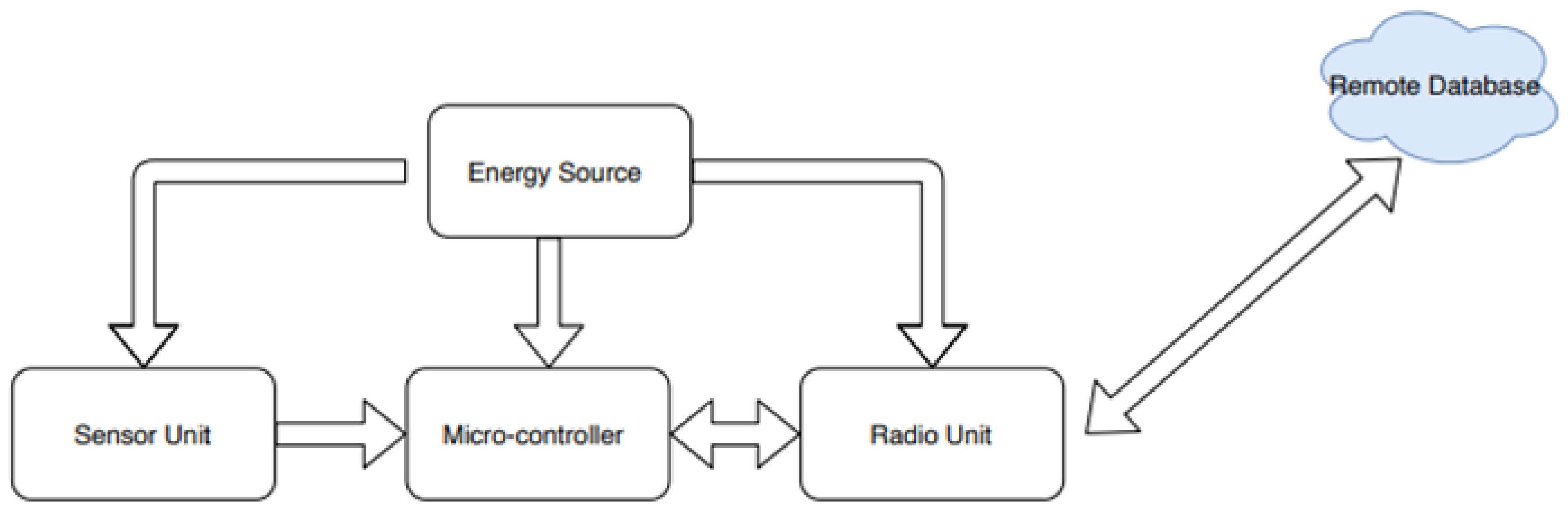
3. Material and Methods

In this work, we did three types of experiments: RSSI recording experiment, current consumption recording experiment, and data transmission experiment. We used SIM800L GSM/GPRS module which was supplied from a 12 V DC power source through an MP1584 adjustable step-down DC to DC converter which helped us to get 4.2 V from 12 V and enough current for the module as it can consume up to 2000 mA [19]. Basically, the experimental set-up has two parts as per Figure 2.

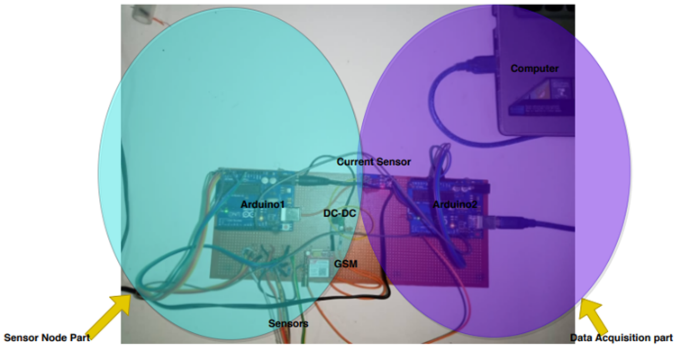
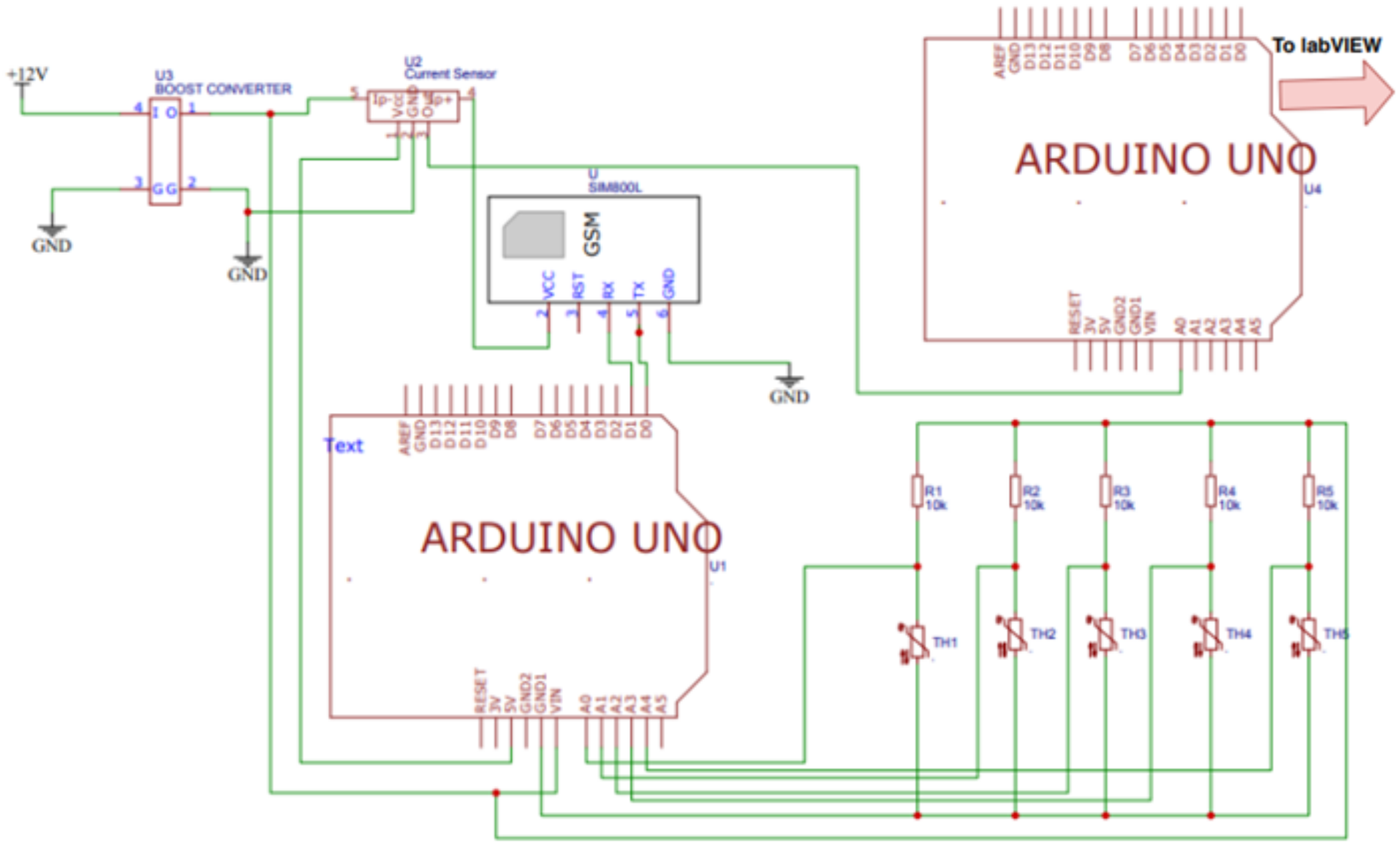
3.1. Current Measuring: Part 1

This is the part that helped us for acquiring data for being analyzed in Python. It is composed of a second Arduino Uno board and a current sensor, details are shown in Figure 3. With this setup, we made a simple LabVIEW program to help us to send data that are coming from the current sensor to an Excel file. From there, data were manually fetched for being analyzed in Python.

3.2. Sensor Node: Part 2

This is the main part of our experiment, which is the one to sense, locally analyze, and send data to a remote database (MySQL DB). It is composed of an Arduino Uno board (Arduino, Turin, Italy) as a micro controller, sensors (20 K NTC Temperature sensors (JINAN BESTAR INC., Jinan, China)) circuitry, and communication mean (GSM/GPRS Module).
The GSM 800L module consumes a maximum of 2 A current so that it can connect to the GSM network [19] with this feature, to supply the module we used an MP1584 (Shenzhen Hengsaisi Technology Co., Ltd., Shenzhen, China) DC-DC converter. Ni LabVIEW, which stands for Laboratory Virtual Instrumentation Workbench, is a National Instrument graphical programming language that is mainly used for data acquisition [20]. In the same way, we have used LabVIEW to help us to acquire, display, and send data to Excel. Figure 4 shows that while data are being sent to Excel, they are displayed on LabVIEW front panel.

3.3. Important Specification about SIM800L

In this paper, SIM800L (SimCom, Shangai, China) GSM module was used as a radio unit. The following Table 1 indicates some important specifications used in this work.

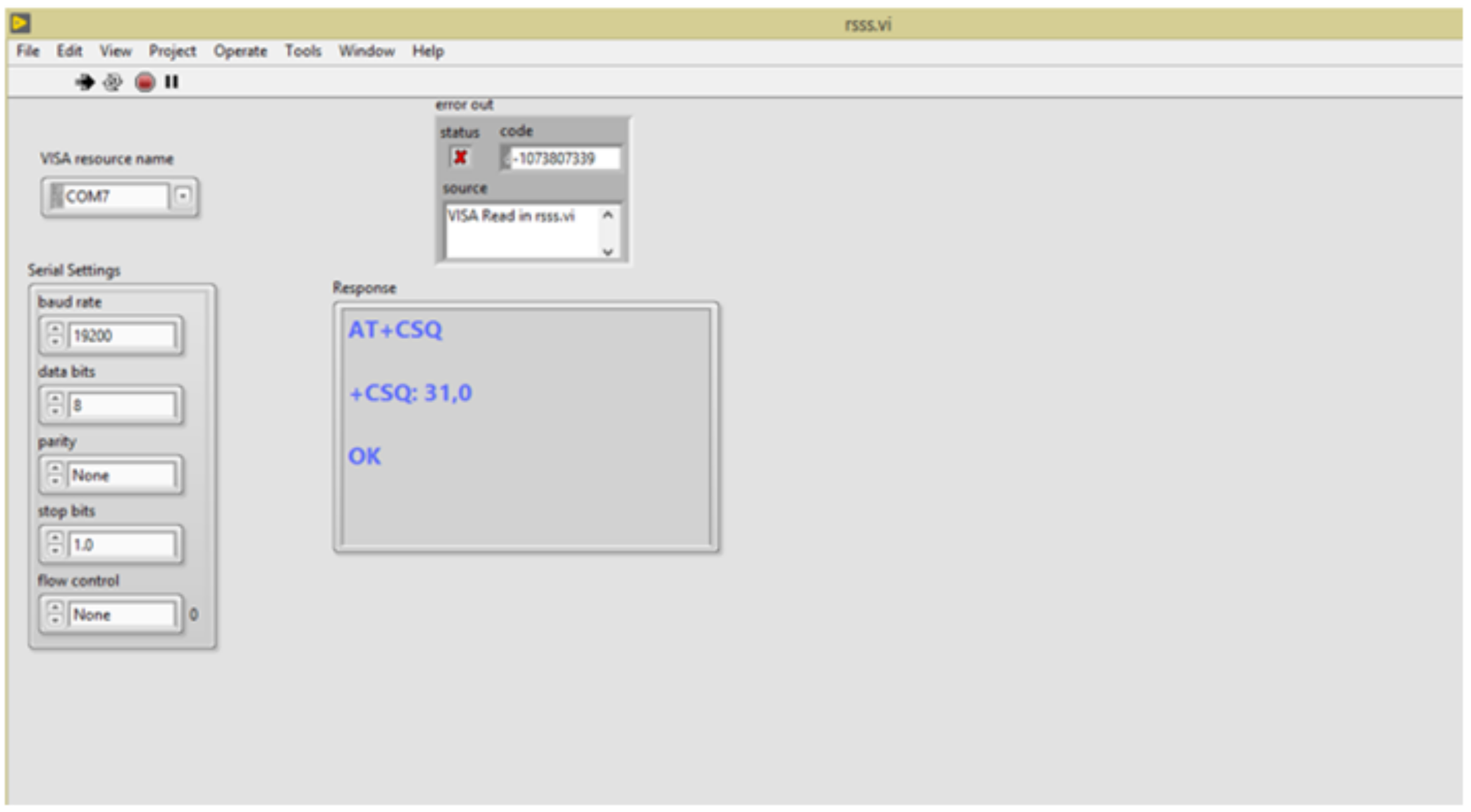
3.4. Useful AT Command for This Research Paper

A microcontroller communicates with GSM module through some commands known as AT commands. The following Table 2 shows AT commands which have been used in this work.

3.5. Battery/Network Life Span

The information about the signal quality in a given area can provide an idea about the energy which is being consumed when the device is trying to connect and send/receive data.

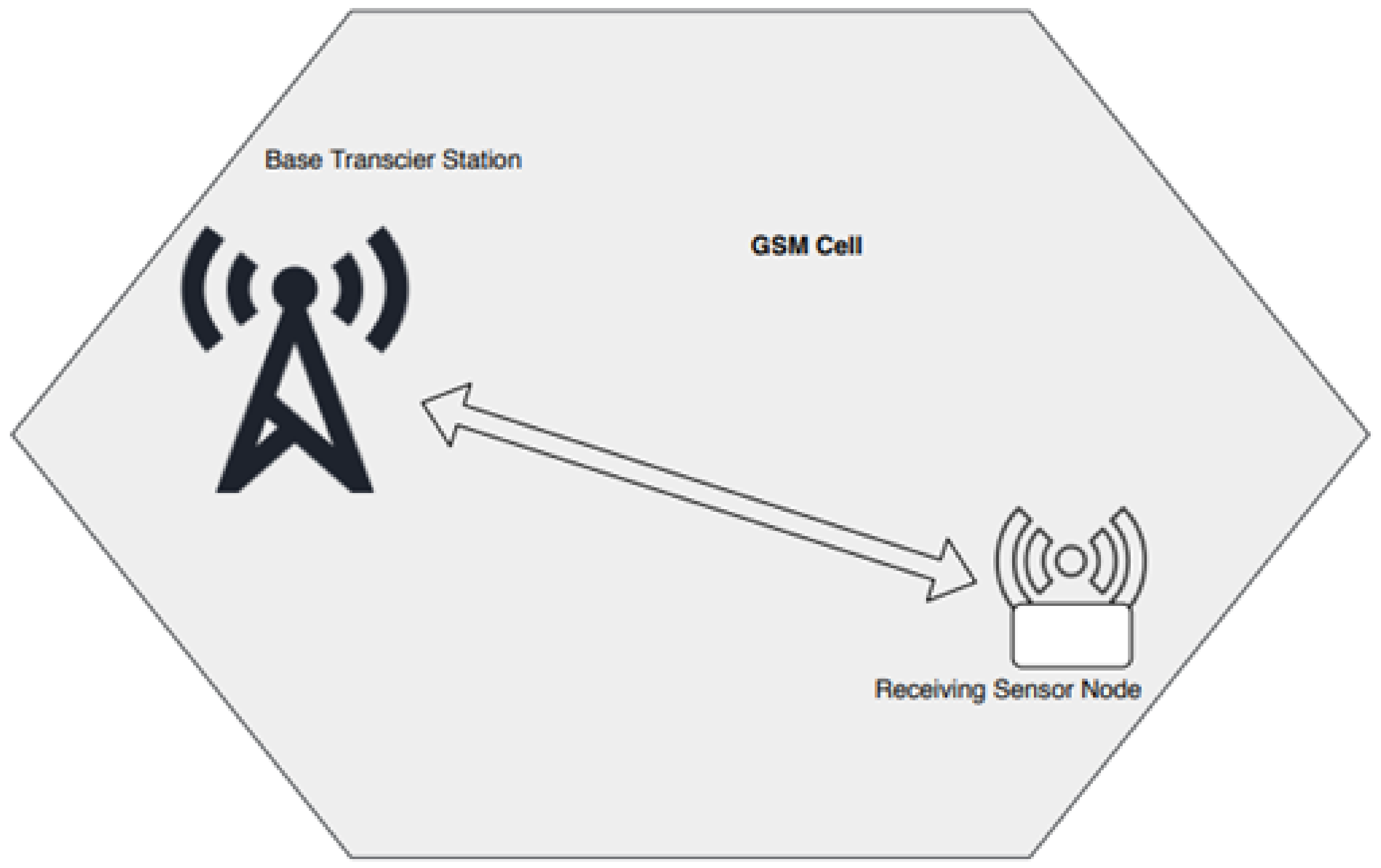
3.6. Experiment Setup

In this paper, we had a target of getting information about the impact of the signal quality represented by received signal quality information (RSSI) on the current consumption of GPRS based sensor nodes. Our experiment had two main parts: the data acquisition part and the data transmission part. Each part has its own microcontroller. This can be seen in Figure 5 below.

3.7. Data Acquisition Part

This is the part in which we collected data about the current consumption for a given location targeting to know the impact of RSSI on the current consumption in that particular area. For each record, we spent 24 h. To achieve this, we used an Arduino Uno based microcontroller, an ACS712 (Shenzhen Hongxuan Electronic Co., Ltd., Shenzhen, China) current sensor, and Ni LabVIEW [21]. The picture for our experiment is shown in Figure 6.
Current data from six locations (with their RSSI values) have been recorded considering four different scenarios.

3.7.1. Scenario1: Reference Current Acquisition

The condition which is taken as reference was a condition when the part 2 (sensor node) was powered off. This time, the current sensor recorded some values and these values were considered as reference current values. We did this for each location because there could be a few changes in electronic circuitry while moving from one location to another. It is a kind of calibration.

3.7.2. Scenario2: GSM Current Acquisition

In this scenario, the GSM module was switched ON and it was connected to GSM network then the corresponding current consumption was recorded too. The current consumed in this situation is the same as sensing current and the current required for connecting to the network.

3.7.3. Scenario3: GPRS Current Acquisition

During this step, with the help of AT commands, the microcontroller for the sensor node was programmed for sending temperature data to a remote database every 20 s, then the current consumption for the whole sensor node was recorded. The total current consumed in this situation is the same as sensing current, the current required for connecting to the network, and the current for sending data to a remote server.

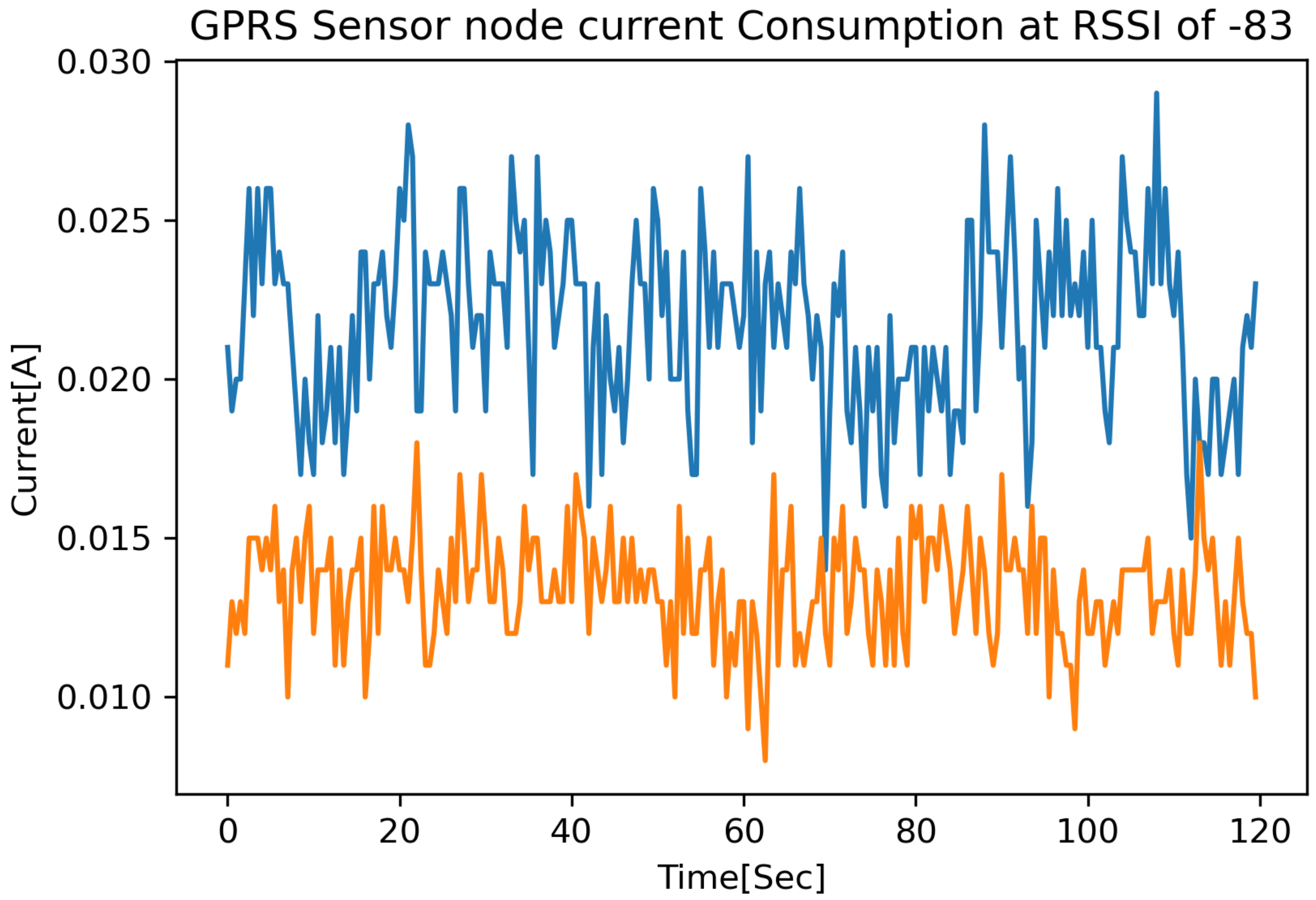
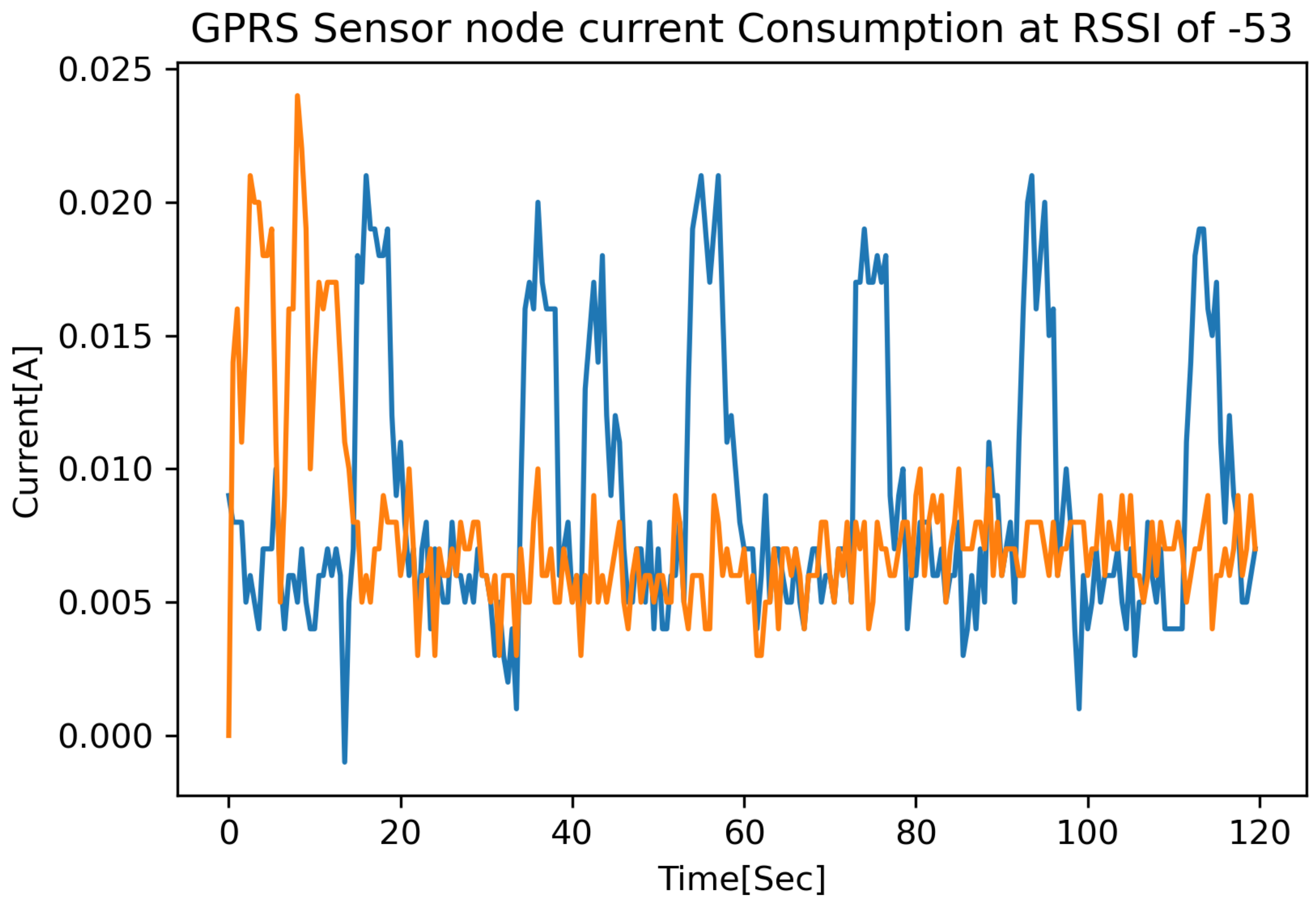
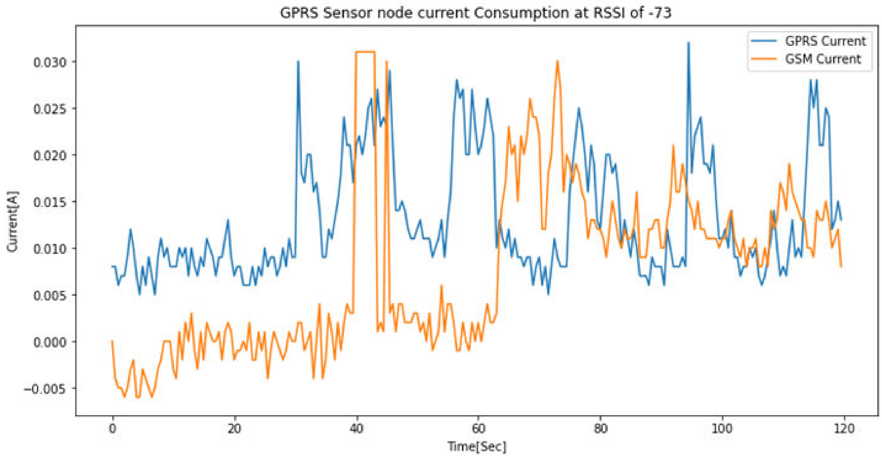
3.7.4. Scenario4: RRSI Acquisition

Received Signal Strength Indicator (RSSI) indicates the strength of the signal power received by a receiving sensor node. RSSI has much application in wireless networks including localization as the distance between the transmitting and receiving devices depends on RSSI. In general, when the distance between those two devices increases, the value of RSSI will reduce [22,23,24,25]. The RSSI value depends on a lot of parameters, including the distance between transmitter and receiver, the geometric orientation of sensors, and the environment characteristics such as rain, temperature, and humidity [25,26,27]; it can also vary with interference from the neighbor network or your own network [28]. Apart from this, the RSSI varies with the presence of a human being [29,30]. The quality of a network depends both on the transmitter and the receiver [31]. On the receiving node, RSSI will depend on the power from the transmitter, the sensibility, the orientation of the antenna toward the transmitter. The information about the received signal power can be calculated by the formulae below [32,33]:
P r = P t . G t . G r ( λ 4 π d ) 2
And RSSI in dBm is generally delivered from the above equation and is given by [32,34]:
R S S I = 10 n l o g ( d ) + A
where P t , G t are taken as the power from the transmitter and the antenna gain respectively in dBm, P r , G r : The power for the receiver and its antenna gain respectively λ and d: The signal wavelength and the distance between transmitter and receiver’s antennas respectively in meters. n: the path-loss constant: This value will vary based on obstacles between the transmitter and receiver. A: the value for RSSI when the distance between the transmitter and receiver is 1 m. If an AT command requesting for the signal quality is sent to a GSM SIM 800 Module, the module will respond will TA (Terminal Adaptor) value. The following Table 3 indicates the relationship between the TA value and the RSSI value [35].
In our experiment, the GSM module will get a signal from the nearby base station (BTS) of the GSM network. For getting information about the RSSI value at a particular location from BTS, through the microcontroller we sent some AT commands.
When AT+CSQ AT command is sent to GSM module, it will respond with the location’s signal quality in the form of TA value. Data information responded by the module is received by the controller and then sent to Microsoft Excel through National Instrument LabVIEW. The acquisition process is shown in Figure 7 and its corresponding LabVIEW dashboard in Figure 8.

3.8. Data Transmission Part

This is the part that can even be called a sensor node. It is made with four subparts: microcontroller, GSM/GPRS Module [36], sensors, and the remote server; the circuit diagram is shown in Figure 9. During this work, we had an idea of sensing the temperature from five different locations and sending them to a remote database using the GPRS protocol. We were sending values every 20 s.

4. Data Analysis and Discussion

The power consumption of the radio unit can be in different operating modes [8]: idle mode which is the mode where the device will be consuming very little current and this time the device does not send or receive any data, with one or two active modes depending on the work. The functional block diagram of sensor node is shown in Figure 10; from this, the total power consumed can be given by the formula below:
P t = P s + P m c r + P r
where P t : Is the total power consumed by the sensor node, P s the total power consumed by the sensor(s), P m c r : The power consumed by the microcontroller unit and P r the total power consumed by the radio unit.
The radio unit power can also be detailed as follows:
P r = P i + P a + P t
where P i is the power when the device is in idle condition, P a active power, when is ready to transmit/receive data and P t the tail power when the module is transmitting/receiving data.

4.1. Sensor Node Current States and Transition

A sensor node has three units which consume power: sensing unit, controller unit, and radio unit. The radio unit is the unit which is consuming a lot of power which is equal to 60% [8] (33% for receiving and 27% for transmitting) and the remaining power is used for sensing/acting and processing units. The graph of Figure 11 shows the current transition of our node from the time it is switched on up to the time when it is transmitting data to a remote database. When the node is switched ON, it took around 60 s consuming low power getting ready to connect to the GSM network and this took an average current of 1.1 mA. We found that the module takes 20 s while jumping from idle state to active mode (the time when the module connects to the GSM network); this transition state consumes an average current of 19.7 mA.
It was seen that when the module connects to the network and transmits data at a constant preprogrammed frequency, it will consume an almost constant current and this will change when there is a change in RSSI value. In our experiment, the active mode has the current for GSM and the current for GPRS and the GPRS current will overshoot each 20 s.
The graph of Figure 12 has been produced in location 3 where the signal quality RSSI was −83 dBm The active mode is the mode where the module has received the AT command for data transmission and it is preparing to send data and the tail mode is the mode during which the module is sending data to the remote server.

4.2. RSSI vs. Current Consumption

Researchers found that when a GSM module in a GSM network has low signal quality, the module will put a lot of effort into trying to get better signal reception; this will make the module consume more power [9,37]. The following Table 4, Table 5, Table 6, Table 7, Table 8 and Table 9 show the impact of the received signal quality on the current consumption of the GSM module. Data have been recorded in six different locations. For each location, we tried to make an average for the consumed current.
The GSM currents were recorded when the module was connected to the network and by disconnecting the cable which links the module to the microcontroller. At this time, the module was not able to receive AT command from the microcontroller.
The graphs for all the six locations show that the GSM current is almost constant and that the GPRS current changes according to how often data are transmitted.
The results from measurements taken from six different locations show that if a GPRS sensor node is located in a place with poor signal quality, the node will consume more current.
Among these six locations, location 2 was the one with poor signal quality (−83 dBm) (Figure 13, Table 5), the node was consuming 17 mA, while location 3 was the one with excellent signal reception( Figure 14 and Table 6), where the sensor node was consuming around 9 mA. Considering location 3 and location 6 with −53 dBm and −63 dB Figure 14 and Table 9) respectively, from those two locations, the results from our experiments show that when the RSSI value reduces with 10 units, the current consumption will increase with 2.91 mA. It can also be seen that between our location with low signal quality (location 2) and location with excellent signal quality (location 3) there is a difference of 30 dBm of RSSI value; this reduction in signal quality made the current double.
We can generally observe that on each graph (Figure 13, Figure 14, Figure 15, Figure 16, Figure 17 and Figure 18), there is an overshoot each 20 s, at this time the module was receiving a GPRS AT command to send data to a remote database. On the same graphs, we can observe that the GPRS protocol consumes more power than GSM protocol. One of the useful services of GSM protocol is transmission of voice which can go to a maximum of 14.4 kbit/s. The GPRS protocol was one of the major developments of GSM network which can support packet switching techniques to accommodate high speed data rate and fast data communication which can go up to 170 kbit/s [38]. In our application there is no voice transmission as there is no microphone or/and speaker connected to the module. However, the module is transmitting some data to a remote database using GPRS protocol; this is why the module consumes more power when it is used in GPRS protocol. It has even been proven by Wataru Toorisaka et al. [39] that the power consumption increases with data rate.
The results from Table 10 consolidate all results from six locations and they are plotted in Figure 19; the TA values of RSSI have been converted using the Table 3.

4.3. SIM 800L Based Sensor None Life Time Estimation

4.3.1. Battery Life Calculation

Even if the RSSI value depends on a lot of factors, when it is measured, we assume that the measured value has been found by taking under consideration its affecting factors. Our data analysis result shows that the average consumption for our sensor node in a particular location depends on the received signal quality at that location; this can be shown on the average currents in Table 10. Considering that our sensor node will be supplied by a small battery of Y Volts with XmAh capacity, let us estimate the lifetime for a sensor node which is working on GPRS protocol. Considering that Lc is the average load current in Amperes, Bc the capacity of the battery in mAh, and the battery lifetime in Hours B l , then the battery life can be given by the battery capacity over the load current [40]
B l = B c L c
Basing on the Equation (5), L c is the total current of the sensor node and is the summation of the current consumed by the sensor unit, microcontroller and radio unit. Then the Equation (5) can be written as:
B l = B c C s + C m c r + C r
where: C s is the sensory unit current, C m c r the microcontroller current, and C r the radio unit current. In our experiment, we tried to record the current consumption of the radio unit and as we recorded for 24 h for each location, we are considering the average current for each location so, C r , the radio unit can be found using the following formula
C r = n = 0 k i k
where: C r is the average radio consumption current at a particular location, k number of measurement, and i the instantaneous current? During our experiment, as we recorded data for 24 h with a waiting time of 500 ms, we made 172,800 measurements for the whole day. Then referring to Equation (7), k = 172,800 and from Table 10, we have Pr form six different locations. Average currents in six different locations are summarized below:
  • Current for Location 1 = 0.016378 A
  • Current for Location 2 = 0.017014 A
  • Current for Location 3 = 0.008890 A
  • Current for Location 4 = 0.012646 A
  • Current for Location 5 = 0.013699 A
  • Current for Location 6 = 0.011800 A

4.3.2. Battery Life Prediction Model for SIM800L Sensor Node

While planning for the development of an IoT network it is necessary to estimate the duration of each network node so that the time on which the battery will be replaced shall be known [6]. It has been found that the GPRS sensor node consumes more power when it is located in a location with bad signal quality and consumes low power when it is located in a location with good signal quality. In this section, we are trying to find a mathematical relationship between the current consumption for a GPRS sensor node at a particular location with the received signal quality.
From the Figure 20, the relationship between the current and RSSI seems to exponentially decay. So, it can be written using the following equation. In this case, the current consumption is our independent variable while the signal quality RSSI is the predictive variable or independent variable and this can be expressed by the following equation:
Y = A e r α
where Y: The average current consumption, A: an initial value and has to be greater than zero r: a decal rate and has to be negative λ : the signal quality or RSSI
The analytical solution for the Equation (8) can be written as:
Y = a + b α + c * l n ( α )
In trying to find a mathematical relationship between the current consumption of a GPRS sensor node with respect to the location where it is placed, we used Python APM (advanced Process Monitor) through its interface GEKKO which is a Python library for machine learning and optimization of mixed-integer and differential equations [41]. We found the solution for the Equation (9) as:
  • a = 0.085966482761
  • b = −0.19094884551
  • c = −0.020681155519
In the end, we tried to calculate the coefficient of determination R 2 to see how our measured data fit our model and the value of R 2 was found to be 0.9231243723176469 which is tending to be unit. This shows that our model is somehow accurate. So, Equation (6) can be written as:
Y = 0.085966482761 0.19094884551 α 0.020681155519 l n ( α )
For our experiment, the above Equation (10), can help us to estimate other currents consumption of our radio unit for other locations in case the RSSI value is known. The RSSI for a particular location can be known using the techniques detailed in Section 3.7.4.
By combining the Equation (10) and equation and Equation (5) and considering that y = Cr (the average current consumed by the radio unit, the Equation (5) can be written as:
B l = B c C s + C m c r + 0.085966482761 0.19094884551 α 0.020681155519 l n ( α )
where:
B l : Battery life in Hours B c : battery capacity in mAh α : the received Signal Strength Information RSSI in dBm Cs, Cmr: the current consumption for sensor circuitry and microcontroller unit respectively.
Considering that the current consumption for the sensory circuitry and the current consumed by the microcontroller are known, the Equation (11) can be considered as our mathematical model which can even help in estimating how long a GPRS sensor node with SIM800L will live at a particular location with known signal quality.

5. Conclusions and Future Work

The results from our experiments show the GSM/GPRS sensor node consumes current in the mA range; this current is not small in WSN or IoT applications. However, in an area like Kigali, Rwanda a country with a lot of hills where the geographical structure does not allow the line of sight communication, building a network using low power sensor nodes like Lora or Sigfox will cost a lot due to a lot of gateways. So, in applications where the line of sight is difficult to achieve and where the GSM network is already in place, GPRS sensor nodes can be used and the cost for building a network will not be expensive as the GSM network is already in place. The quantitative model developed in this paper will help sensor nodes supplied with batteries as it is possible to know how long a battery will last if the information about the signal quality is known and this will finally help to predict when a battery can be replaced. This work has been completed using GSM module. However, we recommend for the future work that a model like the one found in Equation (11) can be found for other modules such as LoRa and Sigfox using the same procedures.

Author Contributions

The ideas presented in this work are a product of contributions by all the authors. The conceptualization of the idea and the development of the manuscript was done by author J.H. in consultation with the supervision team comprising authors M.Z., C.M., E.M., S.K., and K.J. The supervision team played a key role in providing the needed advise and direction throughout the development process of the manuscript. Data curation, Formal analysis, Investigation, Methodology, and Software was done by J.H. with the direct supervision of M.Z. All authors have read and agreed to the published version of the manuscript.

Funding

This research was funded by the African Center of Excellence in Internet of Things (ACEIoT), University of Rwanda.

Conflicts of Interest

The authors declare no conflict of interest.The funder had no role in the design of the study; in the collection, analyses, or interpretation of data; in the writing of the manuscript, or in the decision to publish the results.

Abbreviations

The following abbreviations are used in this manuscript:
IoTInternet of Things
GSMGlobal System for Mobile Communication
GPRSGeneral Packet Radio Services
RSSIReceived Signal Strength Indicator
dBmDecibel
WSNWireless Sensor Network
APMAdvanced Process Monitor
LabVIEWLaboratory Virtual Instrumentation Engineering Workbench
BTSBase Transceiver Station
RTMRemote Temperature Monitor
LEACHLow-Energy Adaptive Clustering Hierarchy
GPSGlobal Positioning Satellite
SNRSignal to Noise Ratio
WIFIWireless Fidelity
DCDirect Current
SSecond
mAMilli Amperes
DBDatabase
MySQLStructured Query Language
ATAttention
TATerminal Adaptor
NoSerial Number
NTCNegative Temperature Coefficient
LoRaLong Range

References

  1. Pietrosemoli, E. IoT Planning and Deployment. In Proceedings of the Workshop on Rapid Prototyping of Internet of Things Solutions, Science Trieste, Trieste, Italy, 21 January–1 February 2019. [Google Scholar]
  2. Prepaid Data SIM Card Wiki Home Page. Available online: https://prepaid-data-sim-card.fandom.com/wiki/Rwanda (accessed on 28 October 2020).
  3. Rodrigues, L.M.; Montez, C.; Budke, G.; Vasques, F.; Portugal, P. Estimating the Lifetime of Wireless Sensor Network Nodes through the Use of Embedded Analytical Battery Models. J. Sens. Actuator Netw. 2017, 6, 8. [Google Scholar] [CrossRef] [Green Version]
  4. Park, C.; Lahiri, K.; Raghunathan, A. Battery discharge characteristics of wireless sensor nodes: An experimental analysis. In Proceedings of the 2005 Second Annual IEEE Communications Society Conference on Sensor and Ad Hoc Communications and Networks, Santa Clara, CA, USA, 26–29 September 2005; pp. 430–440. [Google Scholar] [CrossRef]
  5. Engmann, F.; Katsriku, F.A.; Abdulai, J.; Adu-Manu, K.S.; Banaseka, F.K. Prolonging the Lifetime of Wireless Sensor Networks A Review of Current Techniques. Wirel. Commun. Mob. Comput. 2018, 2018. [Google Scholar] [CrossRef] [Green Version]
  6. Jurenoks, A.; Novickis, L. Analysis of wireless sensor network structure and life time affecting factors. In Proceedings of the 2017 Communication and Information Technologies (KIT), Vysoke Tatry, 4–6 October 2017; pp. 1–6. [Google Scholar] [CrossRef]
  7. Roseline, R.A.; Sumathi, P. Energy Efficient Routing Protocols and Algorithms for Wireless Sensor Networks—A Survey. 2011. Available online: https://www.semanticscholar.org/paper/Energy-Efficient-Routing-Protocols-and-Algorithms-%E2%80%93-Roseline-Sumathi/47810c18daf877a756a3adea891d2cdafe45d94c (accessed on 28 October 2020).
  8. Aderohunmu, F.A.; Paci, G.; Brunelli, D.; Deng, J.; Benini, L. Prolonging the Lifetime of Wireless Sensor Networks Using Light-Weight Forecasting Algorithms. 2013. Available online: https://www.semanticscholar.org/paper/Energy-Efficient-Routing-Protocols-and-Algorithms-https://ieeexplore.ieee.org/document/6529834 (accessed on 28 October 2020).
  9. Ding, N.; Wagner, D.; Chen, X.; Pathak, A.; Hu, Y.C.; Rice, A. Characterizing and modeling the impact of wireless signal strength on smartphone battery drain. ACM SIGMETRICS Perform. Eval. Rev. 2013, 41, 29–40. [Google Scholar] [CrossRef] [Green Version]
  10. Chapre, Y.; Mohapatray, P.; Jha, S.; Seneviratne, A. Received Signal Strength Indicator and Its Analysisin a Typical WLAN System (Short Paper). In Proceedings of the 38th Annual IEEE Conference on Local Computer Networks, Sydney, Australia, 21–24 October 2013. [Google Scholar]
  11. Chang, C. Factors Affecting Capacity Design of Lithium Ion Stationary Batteries. Batteries 2019, 5, 58. [Google Scholar] [CrossRef] [Green Version]
  12. Banguero, E.; Correcher, A.; Pérez-Navarro, Á.; Morant, F.; Aristizabal, A. A Review on Battery Charging and Discharging Control Strategies: Application to Renewable Energy Systems. Energies 2018, 11, 1021. [Google Scholar] [CrossRef] [Green Version]
  13. Jurenoks, A.; Novickis, L. Adaptive Method for Assessing the Life Expectancy of a Wireless Sensor Network in Smart Environments Applications. IFAC PapersOnLine 2016, 49, 25–30. [Google Scholar] [CrossRef]
  14. Elshrkawey, M.; Elsherif, S.M.; Wahed, M.E. An Enhancement Approach for Reducing the Energy Consumption in Wireless Sensor Networks. J. King Saud Univ. Comput. Inf. Sci. 2018, 30, 259–267. [Google Scholar] [CrossRef]
  15. Behera, T.; Samal, U.C.; Mohapatra, S.K. Energy efficient modified LEACH protocol for IoT application. IET Wirel. Sens. Syst. 2017, 8, 223–228. [Google Scholar] [CrossRef]
  16. Yadav, L.; Sunitha, C. Low energy adaptive clustering hierarchy in wireless sensor network (LEACH). Int. J. Comput. Sci. Inf. Technol. 2014, 5, 4661–4664. [Google Scholar]
  17. Tawalbeh, L.A.; Basalamah, A.; Mehmood, R.; Tawalbeh, H. Greener and Smarter Phones for Future Cities: Characterizing the Impact of GPS Signal Strength on Power Consumption. IEEE Access 2016, 4, 858–868. [Google Scholar] [CrossRef]
  18. Balasubramanian, N.; Balasubramanian, A.; Venkataramani, A. Energy Consumption in Mobile Phones: A Measurement Study and Implications for Network Applications. In Proceedings of the 9th ACM SIGCOMM Conference on Internet Measurement, Chicago, IL, USA, 4–6 November 2009; pp. 280–293. [Google Scholar] [CrossRef]
  19. Kanani, P.; Padole, M. Real-time Location Tracker for Critical Health Patient using Arduino, GPS Neo6m and GSM Sim800L in Health Care. In Proceedings of the 4th International Conference on Intelligent Computing and Control Systems (ICICCS), Madurai, India, 13–15 May 2020; pp. 242–249. [Google Scholar] [CrossRef]
  20. Yang, Z.; Wang, S.; Ma, C.; Huang, J. Development of fault diagnosis system for wind power planetary transmission based on labview. J. Eng. 2019, 2019, 9170–9172. [Google Scholar] [CrossRef]
  21. Wang, L.; Tan, Y.; Cui, X. The Application of LabVIEW in Data Acquisition System of Solar Absorption Refrigerator. Adv. Mater. Res. 2012, 16. [Google Scholar] [CrossRef] [Green Version]
  22. Puckdeevongs, A.; Tripathi, N.K.; Witayangkurn, A.; Saengudomlert, P. Classroom Attendance Systems Based on Bluetooth Low Energy Indoor Positioning Technology for Smart Campus. Information 2020, 11, 329. [Google Scholar] [CrossRef]
  23. Nayan, N.P.M.Y.; Hassan, M.F.; Subhan, F. Filters for device-free indoor localization system based on RSSI measurement. In Proceedings of the 2014 International Conference on Computer and Information Sciences (ICCOINS), Kuala Lumpur, Malaysia, 3–5 June 2014; pp. 1–5. [Google Scholar] [CrossRef]
  24. Gorak, R.; Luckner, M.; Okulewicz, M.; Porter, J.; Wawrzyniak, P. Indoor localisation based on GSM signals: Multistorey building study. Mob. Inf. Syst. 2016, 2016, 2719576. [Google Scholar] [CrossRef] [PubMed] [Green Version]
  25. Dolha, S.; Negirla, P.; Alexa, F.; Silea, I. Considerations about the Signal Level Measurement in Wireless Sensor Networks for Node Position Estimation. Sensors 2019, 19, 4179. [Google Scholar] [CrossRef] [Green Version]
  26. Fang, S.; Yang, Y.S. The Impact of Weather Condition on Radio-Based Distance Estimation: A Case Study in GSM Networks With Mobile Measurements. IEEE Trans. Veh. Technol. 2016, 65, 6444–6453. [Google Scholar] [CrossRef]
  27. Nekrasov, M.; Allen, R.; Artamonova, I.; Belding, E. Optimizing 802.15.4 Outdoor IoT Sensor Networks for Aerial Data Collection. Sensors 2019, 19, 3479. [Google Scholar] [CrossRef] [Green Version]
  28. Xie, T.; Jiang, H.; Zhao, X.; Zhang, C. A Wi-Fi-Based Wireless Indoor Position Sensing System with Multipath Interference Mitigation. Sensors 2019, 19, 3983. [Google Scholar] [CrossRef] [Green Version]
  29. Sasiwat, Y.; Jindapetch, N.; Buranapanichkit, D.; Booranawong, A. An Experimental Study of Human Movement Effects on RSSI Levels in an Indoor Wireless Network. In Proceedings of the 12th Biomedical Engineering International Conference (BMEiCON), Ubon Ratchathani, Thailand, 19–22 November 2019; pp. 1–5. [Google Scholar] [CrossRef]
  30. Booranawong, A.; Jindapetch, N.; Saito, H. A system for detection and tracking of human movements using RSSI signals. IEEE Sens. J. 2018, 8, 2531–2544. [Google Scholar] [CrossRef]
  31. Factor Affecting RSSI. Available online: http://www.celtrio.com/ (accessed on 11 June 2020).
  32. Nguyen, N.M.; Tran, L.C.; Safaei, F.; Phung, S.L.; Vial, P.; Huynh, N.; Cox, A.; Harada, T.; Barthelemy, J. Performance Evaluation of Non-GPS Based Localization Techniques under Shadowing Effects. Sensors 2019, 19, 2633. [Google Scholar] [CrossRef] [Green Version]
  33. Shojaifar, A. Evaluation and Improvement of the RSSI-Based Localization Algorithm. Available online: https://www.diva-portal.org/smash/get/diva2:844785/FULLTEXT03.pdf (accessed on 28 October 2020).
  34. Subhan, F.; Khan, A.; Saleem, S.; Ahmed, S.; Imran, M.; Asghar, Z.; Bangash, J.I. Experimental analysis of received signals strength in Bluetooth Low Energy (BLE) and its effect on distance and position estimation. Trans. Emerg. Telecommun. Technol. 2019. [Google Scholar] [CrossRef]
  35. M2MSupport Home Page. Available online: https://m2msupport.net/m2msupport/signal-quality/ (accessed on 12 May 2020).
  36. GPRS with Arduino. Available online: https://hackaday.io/project/27538-remote-data-collection-using-free-gprs (accessed on 2 May 2020).
  37. Why Low Signal Strength Drains More Power; Smartphones Signals and Power Consumption Explained. Available online: https://www.techapprise.com/social/why-low-signal-strength-drains-more-power-smartphones-signals-power-consumption-explained/ (accessed on 19 May 2020).
  38. Ghribi, B.; Logrippo, L. Understanding GPRS: The GSM packet radio service. Comput. Netw. 2000, 34, 763–779. [Google Scholar] [CrossRef] [Green Version]
  39. Toorisaka, W.; Hasegawa, G.; Murata, M. Power Consumption Analysis of Data Transmission in IEEE 802.11 Multi-hop Networks. In Proceedings of the ICNS 2012: The Eighth International Conference on Networking and Servicess, St. Maarten, Netherlands Antilles, 25–30 March 2012. [Google Scholar]
  40. Guo, W.; Healy, W.M. Power Supply Issues in Battery Reliant Wireless Sensor Networks: A Review. Int. J. Intell. Control. Syst. 2014, 19, 15–23. [Google Scholar]
  41. Beal, L.D.R.; Hill, D.C.; Martin, R.A.; Hedengren, J.D. GEKKO Optimization Suite. Processes 2018, 6, 106. [Google Scholar] [CrossRef] [Green Version]
Figure 1. GSM sensor node, in a GSM cell.
Information 11 00524 g001
Figure 2. System Block diagram.
Information 11 00524 g002
Figure 3. Current acquisition process.
Information 11 00524 g003
Figure 4. Current acquisition process LabVIEW graph.
Information 11 00524 g004
Figure 5. System configuration.
Information 11 00524 g005
Figure 6. The picture for the experiment.
Information 11 00524 g006
Figure 7. RSSI acquisition process.
Information 11 00524 g007
Figure 8. RSSI Acquisition LabVIEW graph.
Information 11 00524 g008
Figure 9. System schematic diagram.
Information 11 00524 g009
Figure 10. Sensor Node block diagram.
Information 11 00524 g010
Figure 11. Current transition process.
Information 11 00524 g011
Figure 12. Current consumption in different modes.
Information 11 00524 g012
Figure 13. Current consumption in location 2: RSSI = −83 dBm.
Information 11 00524 g013
Figure 14. Current consumption in location 3: RSSI = −53 dBm.
Information 11 00524 g014
Figure 15. Current consumption in location 1: RSSI = −75 dBm.
Information 11 00524 g015
Figure 16. Current consumption in location 4: RSSI = −73 dBm.
Information 11 00524 g016
Figure 17. Current consumption in location 5: RSSI = −65 dBm.
Information 11 00524 g017
Figure 18. Current consumption in location 6: RSSI = −63 dBm.
Information 11 00524 g018
Figure 19. RSSI vs. current consumption.
Information 11 00524 g019
Figure 20. Mathematical model.
Information 11 00524 g020
Table 1. Important GSM 800L Specification.
FeatureImplementation
Power supply3.4 V–4.4 V
Power savingtypical power consumption in sleep mode is 0.7 mA
Transmitting powerClass 4 (2 W) at GSM 850 and EGSM 900, Class 1 (1 W) at DCS 1800 and PCS 1900
GPRS connectivityGPRS multislot class 12(default), GPRS multislot class 1 12 (option)
Data GPRSGPRS data uplink transfer: max. 85.6 kbps
SIM interfaceSupport SIM card: 1.8 V, 3 V
External antennaFull modem interface with status and control lines, unbalanced, asynchronous, 1200 bps to 115,200 bps
Table 2. Some AT Commands used in this paper.
ApplicationsAT CommandExplanations
AT+CREG?Network cregistration
AT+SAPBR=3,1,Connecting to GPRS
AT+SAPBR=1,1Activation for bear profile
AT Command for GPRSAT+HTTPINITInitialization for HTTP Services
AT+HTTPPARASet HTTP Parameter values
AT+HTTPACTIONHTTP Method action
AT+HTTPREADHTTP Read server response
AT+HTTPTERMTerminate HTTP Service
AT Command for RSSIAT+CSQ=?Signal quality report
Table 3. Mapping between TA value and RSS in dBm.
SNTA ValueRSSI [dBm]Condition
12−109Marginal
23−107Marginal
34−105Marginal
45−103Marginal
56−101Marginal
67−99Marginal
78−97Marginal
89−95Marginal
910−93OK
1011−91OK
1112−89OK
1213−87OK
1314−85OK
1415−83Good
1516−81Good
1617−79Good
1718−77Good
1819−75Good
1920−73Good
2021−71Excellent
2122−69Excellent
2223−67Excellent
2324−65Excellent
2425−63Excellent
2526−61Excellent
2627−59Excellent
2728−57Excellent
2829−55Excellent
2930−53Excellent
Table 4. Current consumption in location 1, RSSI = −75 dBm.
NoTime [s]GSM-Current [A]GPRS-Current [A]RSSI [TA]RSSI [dBm]
100.0110.02319−75
20.50.0130.02820−73
310.0120.02519−75
41.50.0130.02219−75
520.0120.01620−73
......
......
......
172,80086,4000.010.0119−75
Average 0.129225510.01637819.21−75
Table 5. Current consumption in location 2, RSSI = −83 dBm.
NoTime [s]GSM-Current [A]GPRS-Current [A]RSSI [TA]RSSI [dBm]
100.0110.02113−87
20.50.0110.01917−80
310.0110.0218−81
41.50.0140.0218−81
520.0140.02316−79
......
......
......
172,80086,4000.0110.01614−85
Average 0.01170.01701415.20−83
Table 6. Current consumption in location 3, RSSI = −53 dBm.
NoTime [s]GSM-Current [A]GPRS-Current [A]RSSI [TA]RSSI [dBm]
100.0140.00931−53
20.50.0160.00831−53
310.0110.00831−53
41.50.0150.00831−53
520.0210.00531−53
......
......
......
172,80086,4000.0060.00931−53
Average 0.00650.008831−53
Table 7. Current consumption in location 4, RSSI = −73 dBm.
NoTime [s]GSM-Current [A]GPRS-Current [A]RSSI [TA]RSSI [dBm]
100.0110.00819−75
20.50.0070.00818−77
310.0110.00620−73
41.50.0120.00719−75
520.010.00721−73
......
......
......
172,80086,4000.0080.00621−71
Average 0.01020.01264620−73
Table 8. Current consumption in location 5, RSSI = −65 dBm.
NoTime [s]GSM-Current [A]GPRS-Current [A]RSSI [TA]RSSI [dBm]
100.010.01124−65
20.50.0220.00924−65
310.0280.01124−65
41.50.0310.0124−65
520.0280.00924−65
......
......
......
172,80086,4000.0070.00925−63
Average 0.01000.0136924−65
Table 9. Current consumption in location 6, RSSI = −63 dBm.
NoTime [s]GSM-Current [A]GPRS-Current [A]RSSI [TA]RSSI [dBm]
100.0150.03526−61
20.50.0220.03426−61
310.0280.03626−61
41.50.0260.03926−61
520.0310.03426−61
......
......
......
172,80086,4000.0870.12925−63
Average 0.05830.01180025−63
Table 10. Consolidated data for current consumption for all six locations.
LocationAverage RSSI [TA]Average RSSI [dBm]Average Current [A]
Location 119.2−750.016378
Location 215.2−830.017014
Location 330.8−530.008890
Location 424.3−650.012646
Location 519.7−730.013699
Location 625.48−630.011800
Publisher’s Note: MDPI stays neutral with regard to jurisdictional claims in published maps and institutional affiliations.

