Rating Prediction Algorithm Based on User Time-Sensitivity

Abstract

Rating prediction is an important technology in the personalized recommendation field. Prediction results are influenced by many factors, such as time, and their accuracy directly affects the quality of the recommendation. Current time-based collaborative filtering (CF) algorithms have improved the technology of prediction accuracy to a certain extent, but they fail to differentiate the time-sensitivity of different users, which further affects prediction accuracy. To address this issue, we have proposed a rating prediction algorithm based on user time-sensitivity differences. First, we analyzed and modeled the time sensitivities of users, utilized cosine distance and relative entropy to build a judgment function, and then judged the time sensitivities of users based on a voting strategy. Next, we applied the time-sensitivity difference to improve the traditional CF algorithm and optimized the combination of parameters. Finally, we tested our algorithm on standard datasets. The experimental results showed that there are many users who have different sensitivities to time. According to these experimental results, our proposed algorithm has achieved a higher prediction accuracy than other state-of-the-art algorithms.

1. Introduction

With the penetration of information technology into every aspect of people’s personal lives and work, users are not only disseminators of information but also producers of it. With the proliferation of Internet information resources, it becomes more and more difficult for users to find the information they need. Furthermore, the rate of information growth far exceeds people’s ability to process it, resulting in information overload. The collaborative filtering (CF) algorithm is a recommendation method that can help users quickly mine the most valuable information from the massive amount of data sources and provide decision support for users [1,2,3,4,5]. The CF algorithm, proposed by Goldberg [6], is one of the most popular recommendation algorithms. Traditional CF algorithms are generally divided into user-based and item-based CF algorithms. The latter takes into consideration that users’ preferences for items are somewhat similar, and essentially recommend items that are similar to users’ historical preferences. In this study, we calculate item similarities through a user-item rating matrix and then predict the ratings for items that users have not rated.

In general, users’ most recent ratings are more likely to reflect their preference than earlier records or ratings, whose influence on current rating prediction results is relatively minor. For example, user A, who was interested in youth movies one year ago, scored 5 points for High School Musical. However, as time goes by, he grew more fascinated by sci-fi movies, and because he recently watched a number of sci-fi movies, he scored 5 points for Avenger: Endgame. If the changes in the user’s interests and preferences are not taken into account when making rating predictions of new movies for user A, the weights of these two movies in the process of item-based CF recommendation would be the same, which fails to account for the fact that user A currently has a higher preference for sci-fi movies. As a result, the quality of the recommendation will be low. For this reason, researchers have proposed many time-weighted CF algorithms, some of which achieved better results than the traditional CF algorithm [7]. However, they did not consider that different users would have different degrees of sensitivity to time. Some users’ interests and preferences change rapidly with time, while others are relatively stable and less affected by time. Therefore, in this study, we applied the time-sensitivity difference to improve the traditional CF algorithm and proposed a rating prediction algorithm based on user time-sensitivity.

2. Related Work

In recent years, many experts and academics have tried different methods to improve the CF algorithm. Such methods primarily focused on the improvement of similarity calculating methods and the integration of external context (such as time).

2.1. Improvement of Similarity Calculating Methods

In CF, prediction accuracy is a key issue, one that largely influences the prevalence of the recommendation systems. Most of the existing research on CF has focused on designing recommenders with high accuracy. Ratings are determined not only by user preferences but also by the rating habits of users, and the traditional methods of calculating similarity ignored the influence of a rating scale. To solve this problem, Ding et al. [8] proposed converting the user ratings into user preferences and then compared the user preferences to obtain more appropriate similarity scores. Rong Jin et al. [9] presented an approach of normalizing the ratings of different users to the same scale, using an optimization algorithm to automatically compute the weight for different users [10]. While most of the user-item rating matrices are sparse, Ahn et al. [11] proposed an improved similarity calculating method through a heuristic approach, in which the accuracy of CF was improved even when there were few available ratings. Jesús et al. [12] proposed a similarity calculating method based on singular points to extract the contextual user information and calculate the singularity of each item. To increase the accuracy of recommendation, Polatidis et al. [13] improved the CF algorithm by taking the number of items rated jointly by users and the value of Pearson similarity as constraints and adjusted the user similarity according to the corresponding threshold value. Tao et al. [14] divided the dimensions of items into different types and calculated the average preference of all users for these dimensions. The authors then used it to measure the preference sensitivity of each user for each dimension and finally applied the dynamic feature weight to improve the traditional CF algorithm.

2.2. Integration of Time Context

Users’ interests and preferences change dynamically with the passage of time and a change in surroundings. However, traditional CF algorithms only considered the similarity between items and ignored the dynamic changes. In this regard, the current research has been improved in three aspects, the first one of which is based on the time window model. For the first time, Shen et al. [15] considered the rolling time window with the time sequence feature and presented a user-item-time 3D dynamic model with the rolling time window. The authors proposed a dynamic CF recommendation model and algorithm, which processed different ratings according to the time sequence. Finally, they improved the timeliness of the algorithm. The second aspect of improvement was the introduction of a time weight function. Ding et al. [16] proposed a time weight function that used the nonlinear exponential forgetting function to describe the degree of information attenuation, so as to reflect the impact of the ratings in different time periods on the recommendation results. Based on the dynamic time sequence, Koren et al. [17] proposed a CF model for rating prediction, which modeled the change of time over the entire data life cycle and modeled the user’s rating bias of items as a time function, thereby allowing users to change their benchmark ratings. Wei et al. [18] proposed a new algorithm by introducing an interest weight function and a popularity weight function. The algorithm comprised item categories and dynamic time weighting and analyzed the impact of user interest and item popularity that change dynamically with time on recommendations. Zhao et al. [19] proposed time-drifting privacy-preserving CF (TPPCF) based on the privacy protection under the time drift when the authors studied the protection of user privacy and improved the accuracy of rating prediction. They fully considered the characteristics of time drift and assigned a higher weight to the latest rating when calculating user similarities, by adding different time weights to generate relatively accurate results. Based on the nearest neighbor method, Hu et al. [20] integrated the time information into the similarity measurement of the traditional CF algorithm and proposed a time-aware CF algorithm to achieve high-quality web service recommendations. The third aspect of improvement to the CF algorithm was the introduction of a time-series model. For example, Xiao et al. [21] argued that the time-series characteristics of user browsing behaviors were important factors in the prediction model. In this work, the authors proposed a type of CF recommendation algorithm that considered the time-series characteristics of user behaviors.

2.3. Time Context Application for Trust-Based Social Recommendation

In real life, users generally have a tendency to consume items recommended by their friends rather than strangers and trust in friends plays an important role in user’s preferences. Trust between users in social networks emerges as an essential decisive feature when designing social recommender systems, and recommendation quality can be guaranteed based on user interpersonal interests in a social network. To improve the accuracy of recommendation, several social-trust-based recommender systems have recently been suggested. Meo et al. [22] proposed the PTP-MF (pairwise trust prediction through matrix factorization) algorithm, a matrix-factorization approach to predict the intensity of trust and distrust relations in online social networks. The PTP-MF algorithm also incorporated biases in trustor and trustee behavior to make more accurate predictions. Liu et al. [23] presented a contextual trust-oriented social network structure and a concept of quality of trust and proposed a new efficient and effective approximation algorithm D-MCBA based on the Monte Carlo method and optimization search strategies. Time information can be useful in facilitating track in the evolution of user interests and improving recommendation accuracy [24]. In fact, interactions are not perceived the same way over time because some interactions are more important than others when computing an opinion [25]. Taking into account the impact of time, Frikha et al. [26] proposed to integrate the temporal factor in measuring trust between social network friends and developed a Trusted Friends’ Facebook application to demonstrate the importance of time in users’ interactions for determining social trusted friends. Kalaï et al. [27] proposed a level of social trust model, which is founded on novel trust metrics based not only on the users’ interests similarity according to their semantic social profiles but also takes into account the time factor of the users’ active interactions. The experimental results demonstrated how their model produces satisfactory results than other computational models.

The above CF algorithms with time context did not take into account the sensitivity of users to time and held the view that all users’ interests and preferences will change similarly with time. However, in reality, the degree to which the interests and preferences of different users change over time differs. Therefore, in this paper, we analyzed the differences in users’ time sensitivities and divided users into preference-stable users and time-sensitive users, so as to enhance the accuracy of the proposed algorithm. For the preference-stable users, we only needed to use the traditional CF algorithm to predict their ratings. However, for time-sensitive users, it was necessary to premeditate the change of their interests and preferences with time, and therefore we incorporated the time context into the CF algorithm to predict their ratings.

3. Time-Sensitive Detection Algorithm

3.1. Item-Based CF Algorithms

The traditional item-based CF algorithm mainly consists of three phases: constructing ratings matrix R (Table 1), computing similarity of items, and predicting ratings.

Table 1. User-item ratings matrix R.

	I1	I2	I3	…	In
U1	R11	R12	R13	…	R1n
U2	R21	R22	R23	…	R2n
U3	R31	R32	R33	…	R3n
…	…	…	…	…	…
Um	Rm1	Rm2	Rm3	…	Rmn

Phase 1. Constructing ratings matrix R.

Where $U=\{U_1,U_2,U_3,\dots ,U_m\}$ identifies the user set composed of m users, $I=\{I_1,I_2,I_3,\dots ,I_n\}$ identifies the item set composed of n items, R_ij identifies the rating of i-th user to the j-th item, and the value of it is an integer that ranges from 1 to 5. The level of rating implies the degree of user preference to corresponding items; the higher the rating, the more interested the user is in the item.

Phase 2. Similarity computation. There are two main approaches to compute the similarity between two items: cosine similarity and Pearson correlation coefficient.

In cosine similarity, an item is considered as a vector in the m dimension user-space. As in [28], the similarity between different items is measured by calculating the cosine of the angle between different vectors:

$$sim(I_a,I_b)=\cos (\overrightarrow{a},\overrightarrow{b})=\frac{{\displaystyle {\sum }_i^m{R}_{ia}\times R_{ib}}}{\sqrt{{\displaystyle {\sum }_i^m{R}_{ia}{}^2}}\times \sqrt{{\displaystyle {\sum }_i^m{R}_{ib}{}^2}}},$$

(1)

where I_a identifies the a-th item in the item set, R_ia represents the i-th user opinion on the a-th item. I_b identifies the b-th item in the item set, and R_ib represents the i-th user opinion on the b-th item.

The Pearson correlation coefficient standardizes the data and reduces the impact of user differences on ratings [29]. The similarity between different items is measured as follows:

$$sim(I_a,I_b)=\frac{{\displaystyle {\sum }_i^m(R_{ia}-\overline{R_i})\times (R_{ib}-\overline{R_i})}}{\sqrt{{\displaystyle {\sum }_i^m{(R_{ia}-\overline{R_i})}^2}}\times \sqrt{{\displaystyle {\sum }_i^m{(R_{ib}-\overline{R_i})}^2}}},$$

(2)

where $\overline{R_i}$ is the average of the i-th user’s rating.

Phase 3. Rating prediction. In this phase, the prediction of the rating for the given items can be computed by applying the sum of the ratings of the user to items weighted by the similarity between different items as follows:

$$R_{ij}=\frac{{\displaystyle \sum _{c=1}^k{R}_i{}_j\times sim(I_j,I_c)}}{{\displaystyle \sum _{c=1}^{k}sim(I_j,I_c)}},$$

(3)

where I_j identifies the j-th item, I_c identifies the nearest neighbors of it, R_ij represents the i-th user’s opinion on the j-th item, and R_ic represents its opinion on the nearest neighbors.

3.2. Time-Sensitive Detection Algorithm

The key to the item-based CF recommendation algorithm is that it calculates similarities between items, which are based on the user’s preference for items, that is, ratings. Some users’ interests and preferences change dynamically with time and surroundings, which would lead to the change of ratings, and thus affect the accuracy of the CF recommendation algorithm. To solve this problem, we proposed a rating prediction algorithm based on users’ time-sensitive detection.

3.2.1. Time-Sensitive Detection

As shown in Table 2, each rating given by the user has a corresponding timestamp. Therefore, we can construct the timestamp matrix T according to the rating matrix R.

Table 2. User-item timestamp matrix T.

	I1	I2	I3	…	In
U1	T11	T12	T13	…	T1n
U2	T21	T22	T23	…	T2n
U3	T31	T32	T33	…	T3n
…	…	…	…	…	…
Um	Tm1	Tm2	Tm3	…	Tmn

Of these values, T_ij indicates the timestamp that the i-th user rated the j-th item, and 0 indicates that the user did not rate the corresponding item. We then ranked the timestamps in descending order, divided the non-zero timestamps into K time windows, and calculated the prior probability of item types within each time window. For example, $P_{T_1}^a$ indicates the prior probability of type a within time window T₁; similarly, $P_{T_1}^b$ indicates the prior probability of type b within T₁. In our experiments, we randomly selected a time-sensitive user i from the 100K MovieLens dataset and computed the probability distribution of different types that the user watched in five time windows. As shown in Figure 1, Figure 2, Figure 3, Figure 4 and Figure 5, the x-axis represents the types of movies (there are 19 types of movies in the dataset), and the y-axis represents the prior probability of each type in the time window, where its value ranges from 0 to 1.

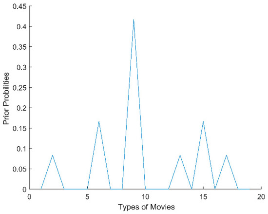
Figure 1. The probability distribution of user i in T₁.

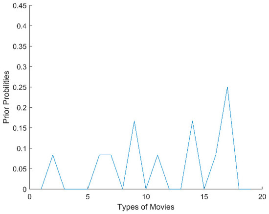
Figure 2. The probability distribution of user i in T₂.

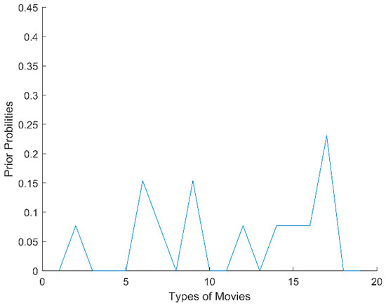
Figure 3. The probability distribution of user i in T₃.

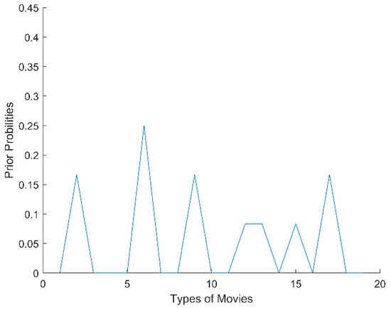
Figure 4. The probability distribution of user i in T₄.

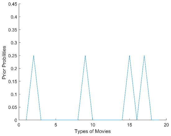
Figure 5. The probability distribution of user i in T₅.

From Figure 1, Figure 2, Figure 3, Figure 4 and Figure 5, we can see that there are obvious differences in the probability distributions within five time windows (T₁ represents the timestamp closest to the current time, T₂ represents the next closest, and so on). Therefore, we planned to use cosine distance and relative entropy to analyze the difference of probability distribution and utilized a voting strategy to judge whether the user’s interests and preferences had changed significantly.

(1) Cosine Distance

In geometry, the cosine is used to measure the difference between two vector directions. As shown in Equation (4), in machine learning this concept is used to measure the difference between sample vectors, and the probability distribution of item types within different time windows can be regarded as sample vectors:

$$D(T_a,T_b)=1-\cos (T_a,T_b)=\frac{{\Vert T_a\Vert }_2{\Vert T_b\Vert }_2-T_a\ast T_b}{{\Vert T_a\Vert }_2{\Vert T_b\Vert }_2},$$

(4)

here, T_a and T_b respectively identify the probability distribution of item types within two time windows a and b and $D(T_a,T_b)$ represents the cosine distance of them. Table 3 shows the cosine distance matrix, which represents the cosine distance of the probability distribution of item types within different time windows.

Table 3. Cosine distance matrix of item type distribution.

	T1	T2	…	Tk
T1	D(T1,T1)	D(T1,T2)	…	D(T1,Tk)
T2	D(T2,T1)	D(T2,T2)	…	D(T2,Tk)
…	…	…	…	…
Tk−1	D(Tk−1,T1)	D(Tk−1,T2)	…	D(Tk−1,Tk)
Tk	D(Tk,T1)	D(Tk,T2)	…	D(Tk,Tk)

(2) Relative Entropy

In probability theory and information theory, relative entropy is often used to describe the difference between two probability distributions. If P(x), Q(x) are the probability distribution of item types within different time windows, then the calculation formula of relative entropy can be expressed as follows:

$$KL\left(P\Vert Q\right)={\displaystyle \sum P\left(x\right)}\log \frac{P\left(x\right)}{Q\left(x\right)}.$$

(5)

Relative entropy is a type of asymmetric measure. In general, $KL\left(P\Vert Q\right)$ and $KL\left(Q\Vert P\right)$ are not equal, that is to say, they are asymmetric, which cannot be directly applied to distance measurements. Therefore, as shown in (6), we used the average value of two-way relative entropy to construct a distance calculation formula based on relative entropy:

$$KL(P,Q)=\frac{KL\left(P\Vert Q\right)+KL\left(Q\Vert P\right)}{2}.$$

(6)

Table 4 is the relative entropy matrix, which represents the relative entropy of the probability distribution of item types within different time windows.

Table 4. The relative entropy matrix of the item type distribution.

	T1	T2	…	Tk
T1	KL(T1,T1)	KL(T1,T2)	…	KL(T1,Tk)
T2	KL(T2,T1)	KL(T2,T2)	…	KL(T2,Tk)
…	…	…	…	…
Tk−1	KL(Tk−1,T1)	KL(Tk−1,T2)	…	KL(Tk−1,Tk)
Tk	KL(Tk,T1)	KL(Tk,T2)	…	KL(Tk,Tk)

Using cosine distance as an example, and based on voting strategy, the voting method is used to judge the users’ time sensitivities. First, we constructed (7) to calculate the threshold:

$$\theta =\frac{{\displaystyle \sum _{i=1}^m(D{(T_a,T_b)}_{\max }+D{(T_a,T_b)}_{\min })}}{2m},$$

(7)

where $D(T_a,T_b)$ represents the maximum value in any user’s cosine distance matrix, while $D{(T_a,T_b)}_{\min }$ represents the minimum value, and m represents the number of users. Then we judged the user’s time-sensitivity according to the indicator function, as shown in Equation (8):

$$S_u=f(\lambda )=\{\begin{array}{cc}0,& \lambda <1\\ 1,& \lambda \ge 1\end{array},$$

(8)

here

$$\lambda =\frac{N_{\theta }^{+}}{N-N_{\theta }^{+}},$$

(9)

where N represents the number of all elements in the distance matrix and $N_{\theta }^{+}$ represents the number of $D(T_a,T_b)\ge \theta$. When $N_{\theta }^{+}$ is the majority, that is, $\lambda \ge 1$, we considered the user to be a time-sensitive user, which is marked as $S_u=1$. However, if we took the user to be preference stable, it is marked as $S_u=0$. The method of calculating threshold and judging time-sensitivity with relative entropy is similar to this and need not be discussed in detail.

3.2.2. Time Function

The above analysis shows that the interests and preferences of time-sensitive users always change dynamically with time, and the closer to the current timestamp, the better the rating can reflect their current interests and preferences.

The German psychologist Hermann Ebbinghaus, a pioneer in the study of memory, put forward the Ebbinghaus forgetting curve, which indicates that people begin to forget knowledge after they learn it, that the amount of knowledge that they can remember gradually decreases, and the forgetting speed changes nonlinearly from fast to slow. Compared with the interest and preference change law of time-sensitive users, the user’s interest decay law and forgetting curve law show some similarities. Therefore, we simulated the attenuation rule of user interest by time weighting, that is, giving different weights to the ratings. The corresponding time function is shown in Equation (10):

$$w(u,i,t)=e^{\frac{t_{\max }-t_{ui}}{T_0}},$$

(10)

where t_ui indicates the timestamp of the rating that rated by the u-th user to the i-th item, w (u, i, t) indicates the weight of it, and t_max indicates the timestamp of the u-th user’s latest rating. T₀ is a half-life parameter, indicates the weight reduction by one-half in T₀ days. Therefore, we proposed a time-weighted method for rating prediction, as shown in Equation (11):

$$R_{ij}=\frac{{\displaystyle \sum _{c=1}^k{R}_{ij}\times sim(I_j,I_c)\times f(S_u)}}{{\displaystyle \sum _{c=1}^{k}sim(I_j,I_c)\times f(S_u)}}$$

(11)

and

$$f(S_u)=\{\begin{array}{cc}w(u,i,t)\hfill & S_u=1\hfill \\ 1\hfill & S_u=0\hfill \end{array}.$$

(12)

From Equation (12), it can be seen that for preference-stable users, the rating prediction result is the same as that of the traditional CF algorithm, and for time-sensitive users, the smaller the distance between the rating timestamp and the current timestamp, the greater the impact on the prediction result and vice versa. This is consistent with the previous analysis.

4. Algorithm Design

4.1. Time-Sensitive Detection Algorithm

Our time-sensitive detection algorithm consists of two parts: one to detect the user’s time-sensitivity, and the other to integrate the time context into the traditional CF algorithm.

(1) User time-sensitivity detection

First, we calculated the cosine distance matrix and the relative entropy matrix of probability distributions of item types within different time windows according to Equations (4) and (6), calculated the value of threshold through the given Equation (7), and then utilized Equation (8) to judge the time-sensitivity of users.

(2) CF algorithm with time context

According to the above analysis, the interests and preferences of time-sensitive users would change significantly with the passage of time. For our proposed algorithm, we first calculated the attenuation of users’ interests with Equation (10), then predicted the ratings with Equation (11). The proposed algorithm is shown in Algorithm 1:

Algorithm 1. Rating Prediction Algorithm Based on User Time-Sensitivity

Input: the ratings matrix R; the number of time windows, K; the number of neighbors, N; the half-life parameter, T0.

Output: predicted rating, ${\stackrel{⌢}{r}}_{ui}$.

1: Initialization, and structure timestamp matrix T.

2: for u = 1, …, m do

3: for i = 1, …, n do

4:  Calculating the similarity between items according to Equations (1) and (2).

5: End for

6: Ranking timestamps in descending order and dividing time windows.

7: for k = 1, …, K do

8:  Calculating item types probability distribution.

9:  Calculating cosine distance matrix according to Equation (4).

10:  Calculating the relative entropy matrix according to Equations (5) and (6).

11:  Judging the user’s sensitivity according to Equations (7)–(9).

12: End for

13: Predicting the rating ${\stackrel{⌢}{r}}_{ui}$ according to Equations (10)–(12).

14: End for

4.2. Parameters Learning Algorithm

In the proposed algorithm, the number of time windows is K, the half-life parameter is T₀ and the number of neighbors is N. Because all three variables have a big impact on rating prediction, it is necessary to find their appropriate values to obtain the optimal prediction results. Nevertheless, because the consumption behavior of individual users is different and the number of historical records of each user is limited, which leads to serious data sparsity, it is difficult to learn the optimal parameters of individual users. Thus, we took the overall perspective into consideration and learned the global optimal parameters that are suitable for specific datasets. If a set of optimal parameters are found, the difference between predicted ratings and actual ratings will be minimal. Therefore, according to the principle of mean absolute error (MAE), we constructed the following function:

$$\begin{array}{c}f(K,N,T_0)=\arg \min MAE\hfill \\ s.t.\{\begin{array}{l}K\in \left\{i\right|i=2,4,\dots ,10\}\\ N\in \left\{j\right|j=1,2,\dots ,20\}\hfill \\ T_0\in \left\{k\right|k=7,30,\dots ,360\}\hfill \end{array}\hfill \end{array}$$

(13)

and

$$MAE=\frac{{\displaystyle \sum _{i=1}^{N\prime }\left|r_{ui}-{\stackrel{⌢}{r}}_{ui}\right|}}{N\prime },$$

(14)

where N’ represents the number of predicted ratings, $r_{ui}$ represents the actual ratings of the users, and ${\stackrel{⌢}{r}}_{ui}$ represents predicted ratings. Based on the observations of our previous experiments, there should be at least two time windows and at most 10 time windows, at most 20 neighbors of items (user consumption records display a long tail phenomenon, if the number of near neighbors is set too large, the noise will be too large), and the half-life parameter T₀ should be set to at most 365 days (based on empirical evidence, the time span of users’ interests and preferences change is about one year, so the half-life parameter is set at 7 days to nearly 1 year). The parameters learning algorithm is as shown in Algorithm 2:

Algorithm 2. Parameters Learning Algorithm

Input: the ratings matrix R; training set of users, U’.

Output: the number of optimal time windows, $f_K$; the number of optimal neighbors, $f_N$; the optimal half-life, $f_{T_0}$.

1: Initialization, K = 2, N = 1, T0 = 7, $f_k=f_N=f_{T_0}=1$, $f_{\min }=10$, MAE = 0

2: while K ≤ 10

3:  while N ≤ 20

4:    while T0 ≤ 360

5:      For each Ui in U’

6:      Call TSDCF(R, K, N, T0)//i.e., call Algorithm 1.

7:        Get Prediction Rating

8:      End for

9:    Calculating MAE

10:     If $f_{\min }$ > MAE then

11:    Update $f_{\min }$, $f_K=K$, $f_{T_0}=T_0$

12:    END if

13:    T0++

14:    End while

15:    N++

16:  End while

17:  K++

18: End while

19: Return $f_K$, $f_N$, $f_{T_0}$

20: END

5. Experiments

5.1. Experiment Design

For this project, we performed experiments on the 100 K MovieLens dataset, which is available from the MovieLens website. It contains 100,000 ratings from 943 users on 1682 movies (each user has at least 20 rating records), and it also contains the rating information, timestamp information and item type attribute information needed by our algorithm. We took the items that were rated by each user at the last time as target items, and then predicted the ratings of them through the proposed algorithm.

In this study, we adopted the most popular metric, mean absolute error (MAE), to evaluate the prediction accuracy of our proposed methods. MAE represents the error between the predicted ratings and the real ratings. A smaller MAE indicates better prediction accuracy [29].

5.2. Experiment (1): The Validity of the Proposed Algorithm

To verify the effectiveness of the proposed algorithm, we compared the time-sensitivity detection CF algorithm (TSDCF) with the traditional CF and the time-weighted CF algorithm (TWCF), which did not take into consideration the difference in users’ time sensitivities. In our experiment, we made K = 5, and T₀ equal to 7 (one week), 30 (one month), 90 (one quarter), 183 (half a year) and 365 (one year), respectively. In the case of the different number of neighbors (N is 5, 10, 15 and 20, respectively), the experimental results with the changes in T₀ are shown in Figure 6, Figure 7, Figure 8 and Figure 9.

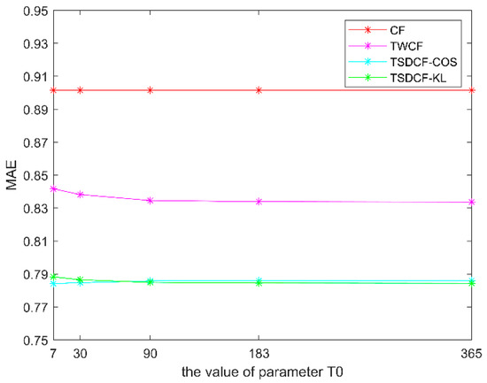
Figure 6. Comparison of algorithms when N = 5.

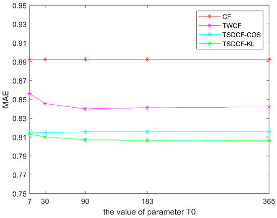
Figure 7. Comparison of algorithms when N = 10.

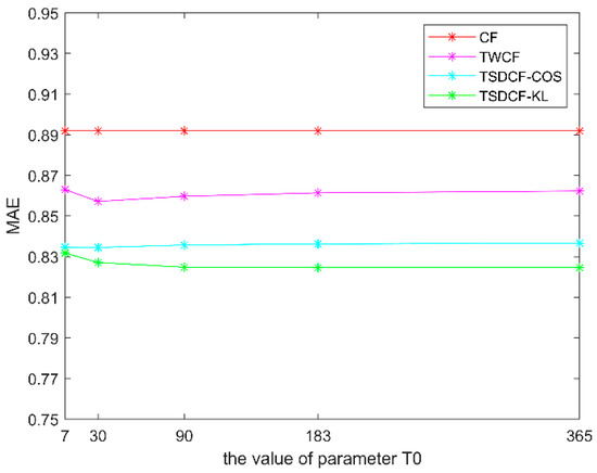
Figure 8. Comparison of algorithms when N = 15.

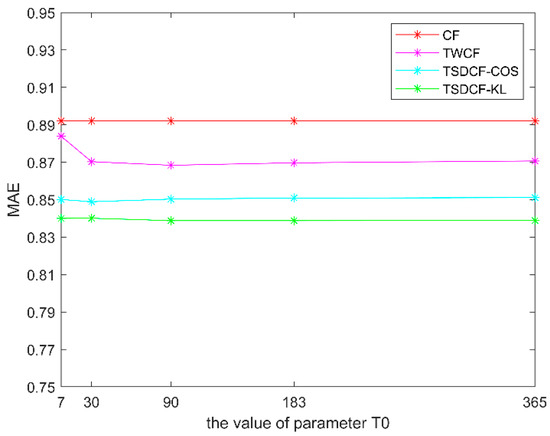
Figure 9. Comparison of algorithms when N = 20.

TSDCF-COS represents the result of the proposed algorithm with cosine distance, while TSDCF-KL represents the result with relative entropy. From Figure 6, Figure 7, Figure 8 and Figure 9, we can see that with different numbers of neighbors, the MAEs of the three algorithms that took into consideration the influence of time context are lower than those of the traditional CF algorithm. Moreover, the results of the proposed algorithm are better than the TWCF algorithm, which does not take into consideration the time-sensitivity of users. When the values of N and T₀ are the same, the prediction error of using relative entropy to measure users’ time sensitivities is slightly smaller than that of using cosine distance. In other words, with the same parameters, the MAE of TSDCF-KL is generally smaller than that of TSDCF-COS. Accordingly, it can be taken that TSDCF-KL is superior to TSDCF-COS. In addition, the MAE will increase with the increase of N, which may be caused by the low similarity between items when N exceeds a certain value or put another way if the number of neighbors is too large, the similarity noise will increase.

5.3. Experiment (2): Parameters Learning Experiments

In Experiment (1), we saw that the algorithm proposed in this paper is better than both the traditional CF algorithm and the time-weighted CF algorithm that did not take the user’s time-sensitivity into consideration. In our experiment, the values of K, T₀, and N have a certain influence on rating prediction. Table 5 displays the results of MAE with different parameters, in which the value of K is respectively 3, 5, and 7, the value of T₀ is, respectively, 7 (one week), 30 (one month), 90 (one-quarter), 183 (half a year), and 365 (one year), and the value of N is, respectively, 5, 10, 15, and 20.

Table 5. Mean absolute error (MAE) with different parameters.

K	T0	N = 5	N = 10	N = 15	N = 20
3	7	0.7745	0.8090	0.8212	0.8398
	30	0.7750	0.8063	0.8199	0.8392
	90	0.7743	0.8056	0.8190	0.8396
	183	0.7748	0.8055	0.8197	0.8402
	365	0.7752	0.8056	0.8201	0.8406
5	7	0.7883	0.8131	0.8318	0.8440
	30	0.7865	0.8102	0.8271	0.8401
	90	0.7849	0.8072	0.8248	0.8388
	183	0.7845	0.8065	0.8246	0.8388
	365	0.7844	0.8062	0.8246	0.8389
7	7	0.7939	0.8158	0.8346	0.8499
	30	0.7938	0.8162	0.8326	0.8471
	90	0.7942	0.8158	0.8324	0.8465
	183	0.7944	0.8161	0.8325	0.8467
	365	0.7944	0.8163	0.8325	0.8467

From Table 5, it can be seen that with different parameter combinations, the value of MAE is changing constantly. It is necessary to find the optimal parameter combinations with the minimum MAE. Therefore, we further optimized the proposed algorithm and carried out parameters learning experiments to obtain the optimal predictions. When T₀ takes different values and MAE is the minimum, the optimal K, N, and corresponding MAE will be as shown in Table 6.

Table 6. Optimal experiment results with different T₀.

T0	K	N	MAE
7	3	5	0.7745
30	4	5	0.7714
90	4	5	0.7701
183	4	5	0.7739
365	4	5	0.7698

Bold figure: The minimum value of MAE.

From Table 6, we can see that when the half-life T₀ = 365 (one year), the MAE receives the minimum value of 0.7698and the corresponding K = 4, N = 5. That is to say, when the number of time windows is 4 and the number of neighbors is 5, the minimum error of the proposed algorithm is 0.7698, which is 14.6% lower than the value of the traditional CF algorithm (0.9015). That is to say, most users’ interests and preferences have changed after one year, at this time, the most suitable value of time windows is 4, and the best number of neighbors is 5.

6. Conclusions and Future Research

Our work leveraged the traditional CF algorithm but took the influence of time context into consideration. The differences in users’ time sensitivities were analyzed, and based on that, we proposed a rating prediction algorithm. The proposed algorithm improved the accuracy of the prediction results. To differentiate and quantify the time sensitivities of different users, we designed a model of user time-sensitivity based on the rating timestamp matrix used to improve the traditional item-based CF algorithms. Furthermore, a parameter learning algorithm was proposed to find the optimal combination of parameters. We verified the effectiveness of the proposed algorithm and obtained the optimal combination of parameters through many experiments on the standard dataset.

In the future, we will use more real datasets to test our algorithm in different fields and attempt to incorporate online testing and application. At the same time, we will further study a strategy, which can automatically select an effective range of values according to different datasets. For example, considering the sparsity of the dataset, the size of time windows for all users was set to the same in this algorithm. However, because, in fact, there are still differences between users, it will be necessary to study the appropriate size of time windows for different users.

References

- Herlocker, J.L.; Konstan, J.A.; Terveen, L.G. Evaluating CF recommender systems. ACM Trans. Inf. Syst. 2004, 22, 5–53. [Google Scholar] [CrossRef]
- Zhang, J.; Lin, Z.; Xiao, B.; Zhang, C. An optimized item-based collaborative filtering recommendation algorithm. In Proceedings of the 2009 IEEE International Conference on Network Infrastructure and Digital Content, Beijing, China, 6–8 November 2009; pp. 414–418. [Google Scholar]
- Wang, X.D.; Sang, J. A Collaborative Filtering Recommendation Algorithm with Time-Adjusting Based on Cloud Model. Comput. Eng. Sci. 2012, 34, 160–163. [Google Scholar]
- Ma, X.; Wang, C.; Yu, Q.; Li, X.; Zhou, X. An FPGA-based accelerator for neighborhood-based collaborative filtering recommendation algorithms. In Proceedings of the2015 IEEE International Conference on Cluster Computing, Washington, DC, USA, 14–17 November 2015; pp. 494–495. [Google Scholar]
- Bobadilla, J.S.; Ortega, F.; Hernando, A.; Bernal, J. A collaborative filtering approach to mitigate the new user cold start problem. Knowl.-Based Syst. 2012, 26, 225–238. [Google Scholar] [CrossRef]
- Goldberg, D.; Nichols, D.; Oki, B.M.; Terry, D. Using collaborative filtering to weave an information tapestry. Commun. ACM 1992, 35, 61–71. [Google Scholar] [CrossRef]
- Cheng, S.; Liu, Y. Time-aware and grey incidence theory based user interest modeling for document recommendation. Cybern. Inf. Technol. 2015, 15, 36–52. [Google Scholar] [CrossRef]
- Ding, Y.; Li, X.; Orlowska, M.E. Recency-based collaborative filtering. In Proceedings of the 17th Australasian Database Conference, Hobart, Australia, 16–19 January 2006; Australian Computer Society, Inc.: Darlinghurst, Australia, 2006; Volume 49, pp. 99–107. [Google Scholar]
- Jin, R.; Si, L. A study of methods for normalizing user ratings in collaborative filtering. In Proceedings of the 27th Annual International ACM SIGIR Conference on Research and Development in Information Retrieval, Sheffield, UK, 25–29 July 2004; pp. 568–569. [Google Scholar]
- Jin, R.; Chai, J.Y.; Si, L. An automatic weighting scheme for collaborative filtering. In Proceedings of the 27th Annual International ACM SIGIR Conference on Research and Development in Information Retrieval, Sheffield, UK, 25–29 July 2004; pp. 337–344. [Google Scholar]
- Ahn, H.J. A new similarity measure for collaborative filtering to alleviate the new user cold-starting problem. Inf. Sci. 2008, 178, 37–51. [Google Scholar] [CrossRef]
- Bobadilla, J.; Ortega, F.; Hernando, A. A collaborative filtering similarity measure based on singularities. Inf. Process. Manag. 2012, 48, 204–217. [Google Scholar] [CrossRef]
- Polatidis, N.; Georgiadis, C.K. A dynamic multi-level collaborative filtering method for improved recommendations. Comput. Stand. Interfaces 2017, 51, 14–21. [Google Scholar] [CrossRef]
- Tao, L.; Cao, J.; Liu, F. Dynamic feature weighting based on user preference sensitivity for recommender systems. Knowl.-Based Syst. 2018, 149, 61–75. [Google Scholar] [CrossRef]
- Yu-pu, S.J.Y. Dynamic Collaborative Filtering Recommender Model Based on Rolling Time Windows and its Algorithm. Comput. Sci. 2013, 40, 206–209. [Google Scholar]
- Ding, Y.; Li, X. Time weight collaborative filtering. In Proceedings of the 14th ACM International Conference on Information and Knowledge Management, Bremen, Germany, 31 October–5 November 2005; pp. 485–492. [Google Scholar]
- Koren, Y. Collaborative filtering with temporal dynamics. In Proceedings of the 15th ACM SIGKDD International Conference on Knowledge Discovery and Data Mining, Paris, France, 28 June–1 July 2009; pp. 447–456. [Google Scholar]
- Wei, S.; Ye, N.; Yang, X. Collaborative Filtering Algorithm Combining Item Category and Dynamic Time Weighting. Comput. Eng. 2014, 6, 45. [Google Scholar]
- Zhao, F.; Xiong, Y.; Liang, X.; Gong, X.; Lu, Q. Privacy-preserving collaborative filtering based on time-drifting characteristic. Chin. J. Electron. 2016, 25, 20–25. [Google Scholar] [CrossRef]
- Hu, Y.; Peng, Q.; Hu, X. A time-aware and data sparsity tolerant approach for web service recommendation. In Proceedings of the 2014 IEEE International Conference on Web Services, Anchorage, AK, USA, 27 June–2 July 2014; pp. 33–40. [Google Scholar]
- Xiao, Y.; Ai, P.; Hsu, C.H.; Wang, H.; Jiao, X. Time-ordered collaborative filtering for news recommendation. China Commun. 2015, 12, 53–62. [Google Scholar] [CrossRef]
- Meo, P.D. Trust Prediction via Matrix Factorisation. ACM Trans. Internet Technol. 2019, 19, 44. [Google Scholar] [CrossRef]
- Liu, G.; Liu, A.; Wang, Y.; Li, L. An efficient multiple trust paths finding algorithm for trustworthy service provider selection in real-time online social network environments. In Proceedings of the 2014 IEEE International Conference on Web Services, Anchorage, AK, USA, 27 June–2 July 2014; pp. 121–128. [Google Scholar]
- Campos, P.G.; Díez, F.; Cantador, I. Time-aware recommender systems: A comprehensive survey and analysis of existing evaluation protocols. User Model. User-Adapt. Interact. 2014, 24, 67–119. [Google Scholar] [CrossRef]
- Haydar, C.; Boyer, A.; Roussanaly, A. Time-aware trust model for recommender systems. In Proceedings of the International Symposium on Web AlGorithms, Deauville, France, 2–4 June 2015. [Google Scholar]
- Frikha, M.; Mhiri, M.; Zarai, M.; Gargouri, F. Time-sensitive trust calculation between social network friends for personalized recommendation. In Proceedings of the 18th Annual International Conference on Electronic Commerce: E-Commerce in Smart Connected World, New York, NY, USA, 17–19 August 2016; p. 36. [Google Scholar]
- Kalaï, A.; Wafa, A.; Zayani, C.A.; Amous, I. LoTrust: A social Trust Level model based on time-aware social interactions and interests similarity. In Proceedings of the 2016 14th Annual Conference on Privacy, Security and Trust (PST), Auckland, New Zealand, 12–14 December 2016; IEEE: West Lafayette, IN, USA, 2016; pp. 428–436. [Google Scholar]
- Karahodza, B.; Supic, H.; Donko, D. An Approach to design of time-aware recommender system based on changes in group user’s preferences. In Proceedings of the 2014 X International Symposium on Telecommunications (BIHTEL), Sarajevo, Bosnia and Herzegovina, 27–29 October 2014; IEEE: West Lafayette, IN, USA, 2014; pp. 1–4. [Google Scholar]
- Li, K.; Zhou, X.; Lin, F.; Zeng, W.; Wang, B.; Alterovitz, G. Sparse online collaborative filtering with dynamic regularization. Inf. Sci. 2019, 505, 535–548. [Google Scholar] [CrossRef]
© 2019 by the authors. Licensee MDPI, Basel, Switzerland. This article is an open access article distributed under the terms and conditions of the Creative Commons Attribution (CC BY) license (http://creativecommons.org/licenses/by/4.0/).