In order to improve the efficiency of outlier detection and avoid the influence of the nearest neighbor parameters on the accuracy of the algorithm, we propose a parameter-free outlier detection algorithm. The parameter-free outlier detection algorithm mainly consists of two stages. Firstly, we propose a DOM method to initialize the original data. In this method, we propose the concepts of partition function (P) and threshold function (T); and filtering the data clusters in which density is greater than a specific threshold, we obtain the initialized datasets. Then, we establish a parameter-free detection method, in which we introduce the concept of the number of residual neighbors and determine outliers via observing the changes of the number of residual neighbors of data points and the size of data clusters.
3.1. Dataset Optimization Method
Each data point exists in different forms, including large data clusters, small data clusters, and sparsely distributed outliers. The traditional outlier detection algorithm needs to calculate the outlier value of each data point, which leads to high time complexity of the algorithm.
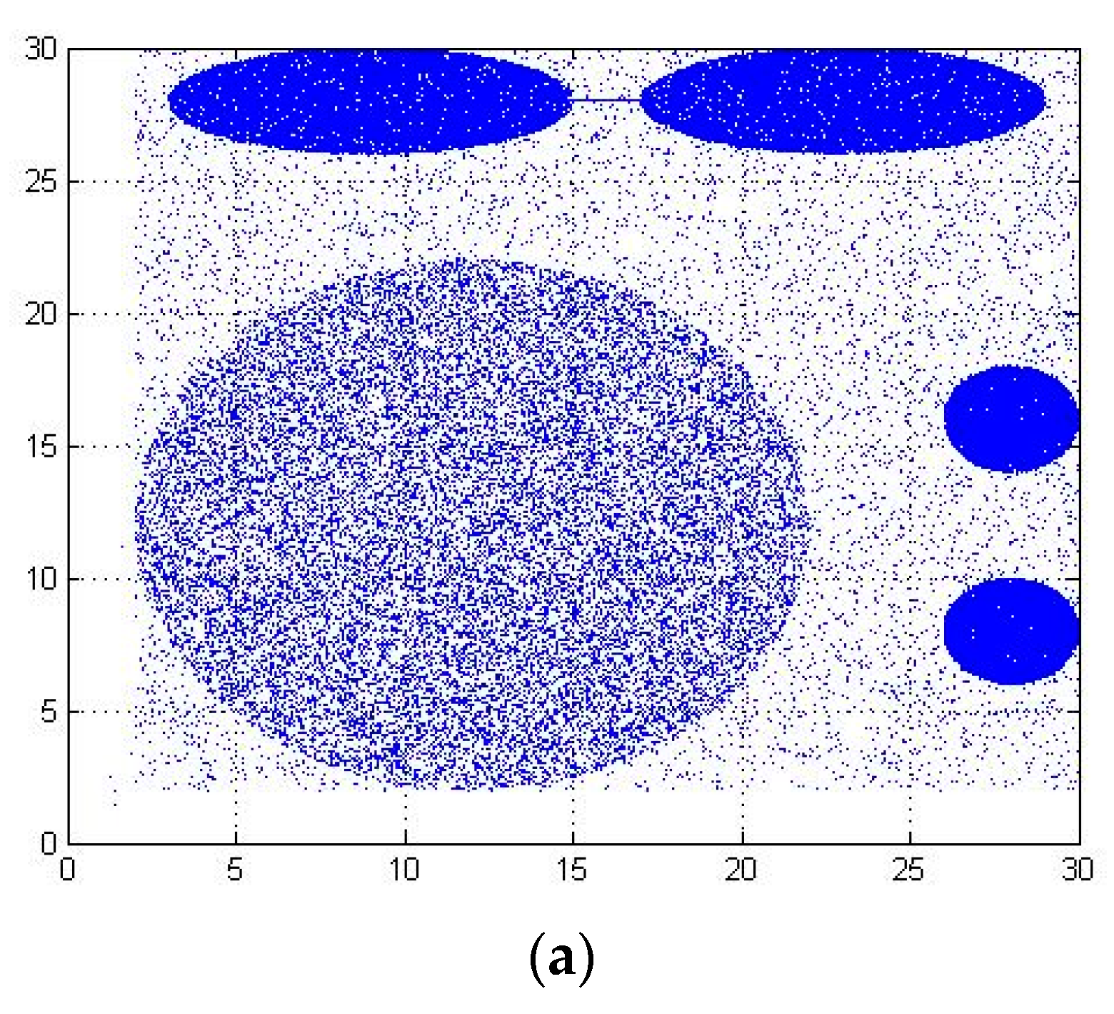
As shown in
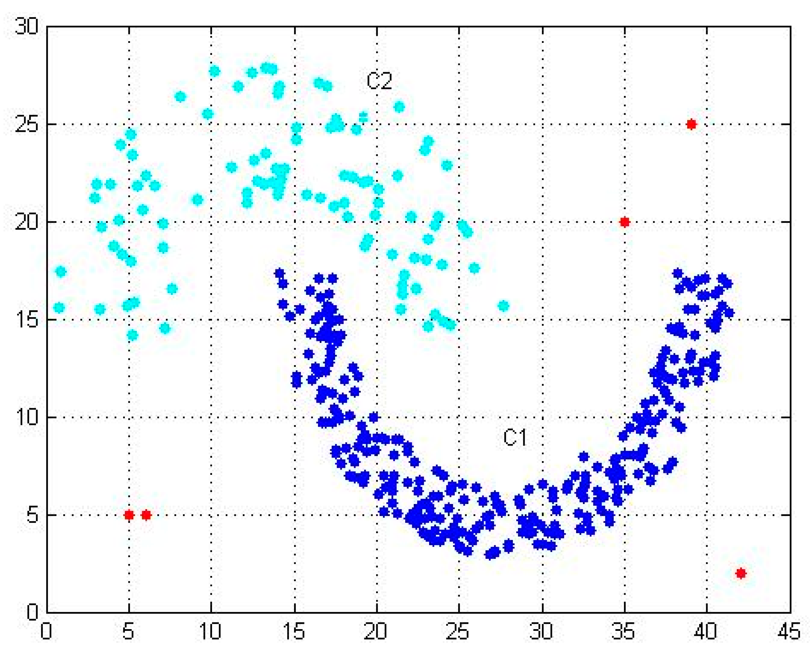
Figure 1, the blue data points are C1 dense clusters, and the blue-green data points are C2 sparse clusters. They are normal data clusters in the dataset. Red data points are outliers. The density-based outlier detection algorithm needs to calculate the outlier degree of each data point (C1 cluster, C2 cluster, outlier), resulting in a high time complexity for the algorithm.
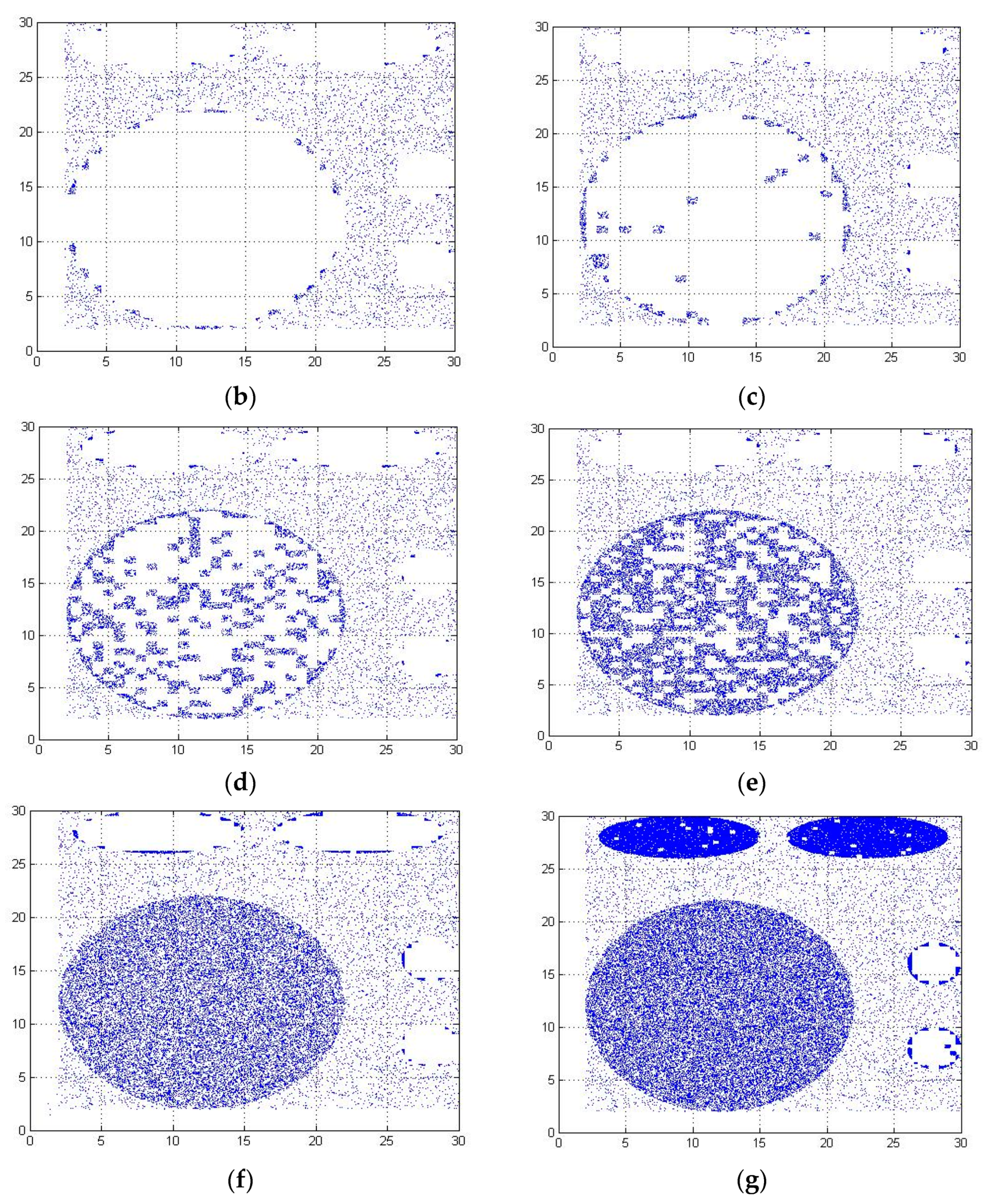
According to the distribution characteristics of outliers and the problem of high time complexity in detection, our paper proposes a dataset optimization method (DOM). In the dataset optimization method, we propose two new functions: partition function (P) and threshold function (T), which are used to determine the data space partition and threshold, and finally achieve the effect of initializing the dataset without parameters. As shown in
Figure 1, the large data cluster (C1) is filtered by the DOM, which ensures that the amount of data entering the next stage is small. On the other hand, it improves the efficiency of the algorithm and requires low time complexity.
To describe the process of dataset optimization, we use Algorithm 1 to describe two-dimensional datasets. In Algorithm 1, we first input the original dataset. Then, in step 1, we use the value of partition function to complete spatial partition and regional data point statistics. In step 2, we compare the number of data points and the size of the threshold function for each region and then determine whether each region is dense or non-dense. If the number of data points in the region is larger than the threshold function, the region is dense. We initialize the data points in this area. Otherwise, the area is not dense. We preserve non-dense data points in the dataset. Finally, we completed the dataset optimization method to obtain candidate datasets as follows:
| Algorithm 1. Dataset optimization method |
| input: Original Dataset {O} |
| output: Candidate Dataset{C} |
| initialize: {c} = ∅ |
| step1: |
| use function Split Area() split space area |
| Block Num = Split Area({o}) |
| //block Num is the number of Blocks |
| for I = 1, 2, … block Num do |
| Num = Count Point Num() |
| End for |
| step2: |
| initialize threshold T |
| for I = 1, 2, … block Num, do |
| get current block points: { block I } |
| get the number num of current block |
| if(num<T) |
| this block area is non-dense set |
| {c} = {c}∪{ block I } |
| else |
| { block I } = ∅ |
| endif |
| endfor |
We propose two new functions, partition function, and threshold function, to partition the data space and achieve the effect of initializing datasets without parameters.
The partition function determines the partition of space and divides N data points into different regions according to their respective positions. If the dataset is large, the partition area should be relatively large. Otherwise, since the number of partition areas are so few that the data in each partition is too dense, the outliers belonging to the abnormal areas are wrongly distributed to the normal area. When the dataset is small, the partition area should be relatively small.
Threshold function is a measure to evaluate whether the areas in the partition function are dense areas. When the number of data points in each region is greater than the threshold function, the data cluster is dense. Then, we filter such dense data clusters to obtain the initialized candidate datasets.
In order to determine the reasonable partition function and threshold function, we verify the data size of 1–100,000 datasets. We express it mathematically as follows.
denotes the dataset; is the number of N; P is the number of rows or columns partitioned by regions; and T refers to the size of threshold function.
The partition function is used to partition the dataset. If the dataset is large, the partition area should increase accordingly. If the dataset is small, the partition area should be correspondingly smaller.
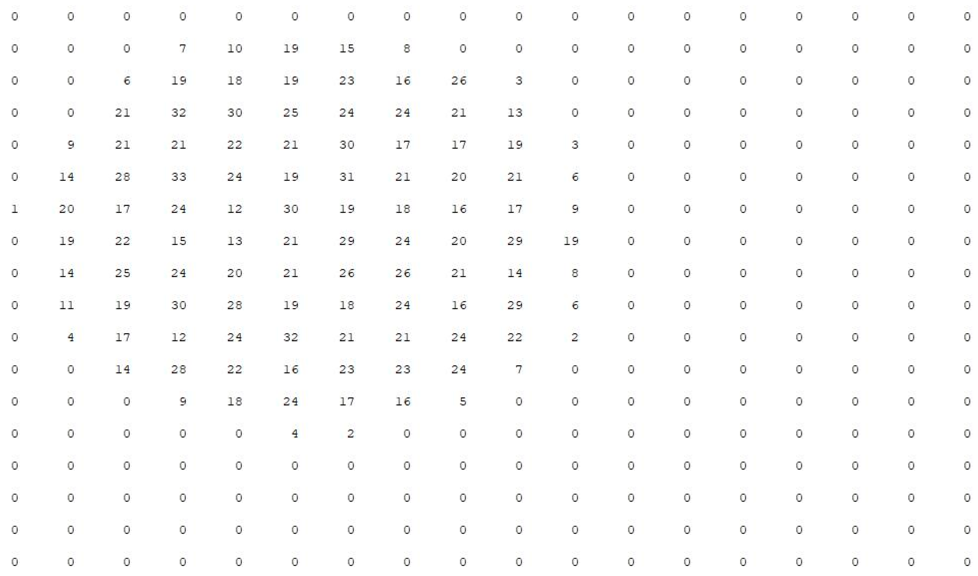
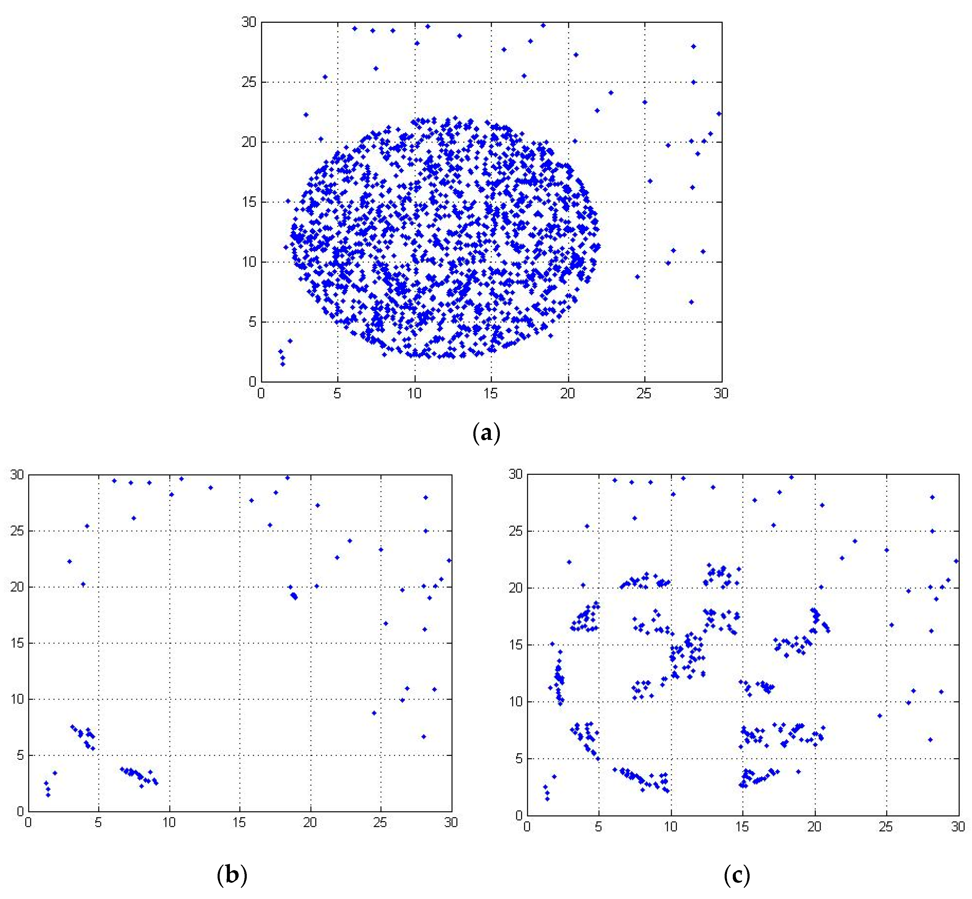
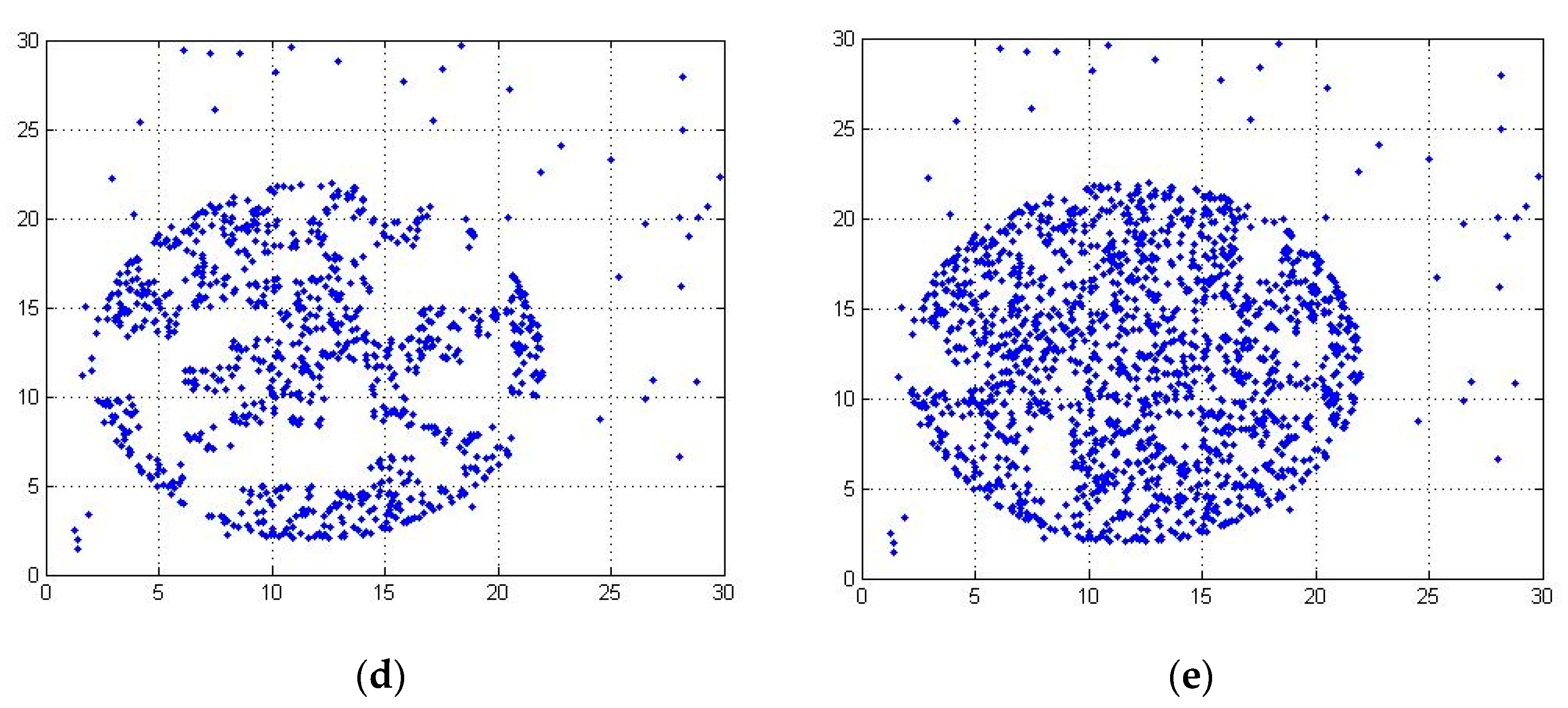
Figure 2 shows the distribution of datasets with |N| = 2000 when the partition function is 18.
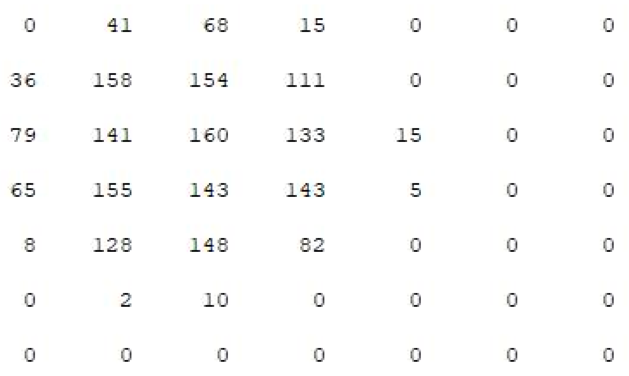
Figure 3 shows the distribution of datasets with |N| = 2000 when the partition function is 7. When the partition function is 7, the dataset of each region is too dense, and the possible abnormal data points are wrongly divided into a region with normal points. Therefore, the size of the partition function and threshold function should change with the change of dataset. Therefore, we propose the definition of partition function P.
The dataset is divided by a partition function. If the data points in the datasets are evenly distributed in the partitioning area, the definition of threshold function T1 can be obtained, as shown in Formula (5).
Since the number of outliers is unknown in advance, it is impossible to judge correctly only by threshold function T1. Therefore, we propose the definition of threshold function T2.
The threshold partition function plays an important role in dataset optimization. If the threshold function value is too large, the dense data in the dataset will be over-preserved. If the threshold function value is small, the sparse datasets and even the outliers in the datasets are filtered out. Neither of them can achieve the effect of initialization filtering. We propose a threshold function that can be applied to many datasets.
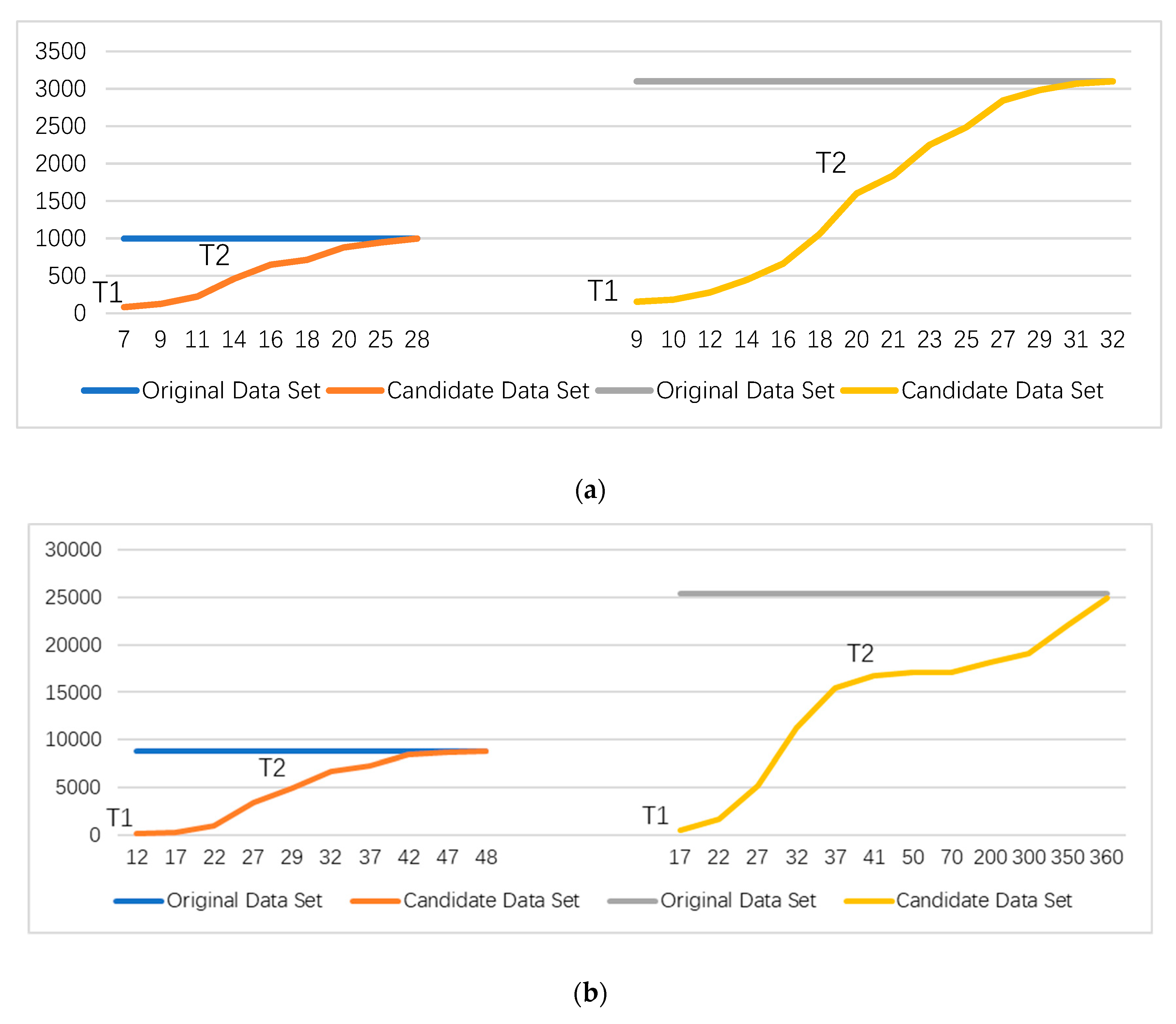
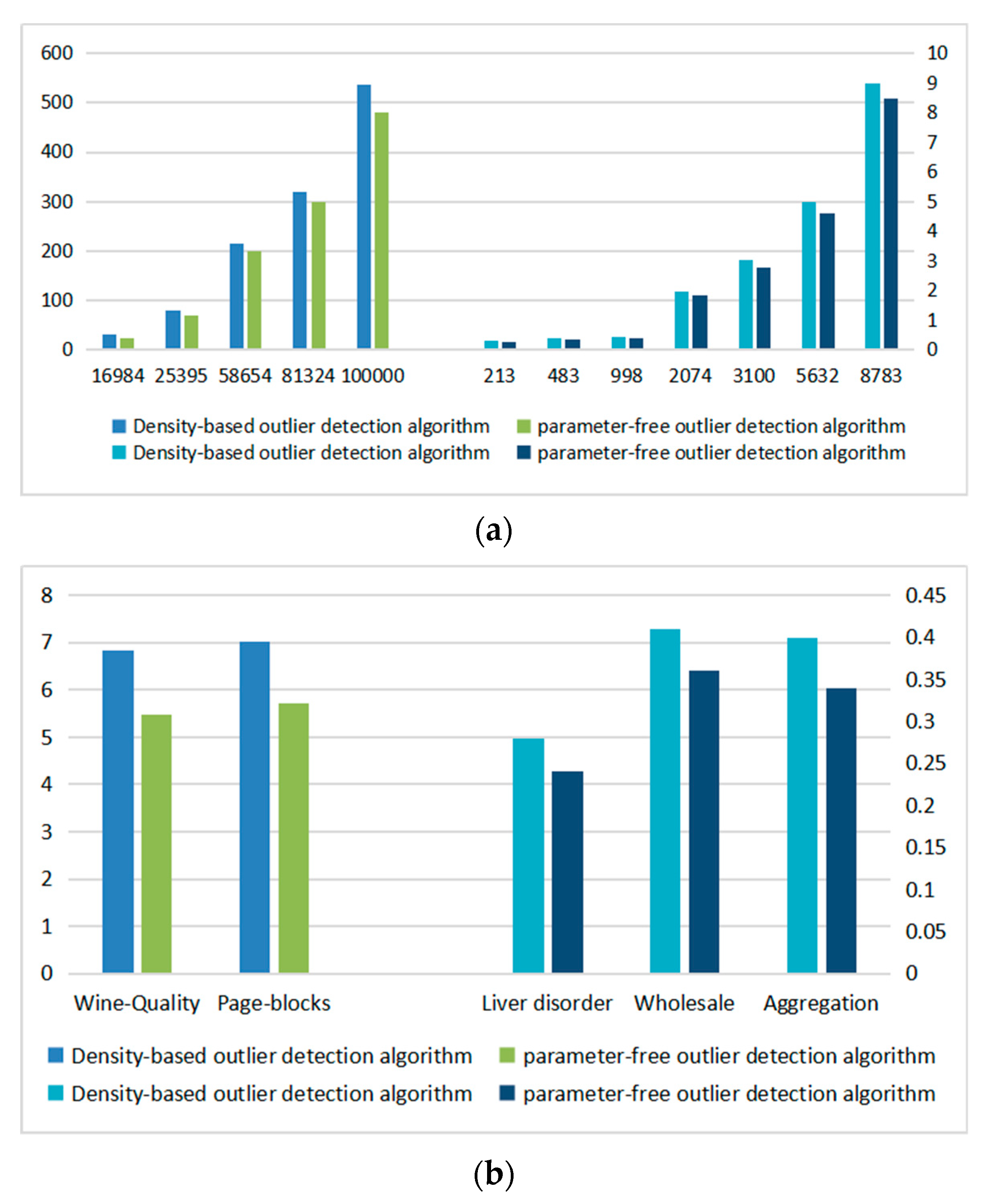
Figure 4 shows the data volume comparison curve between the original dataset and the candidate dataset.
Figure 4a shows the original datasets with data amounts of 998 and 3100. With the increase of the threshold function, the amount of data in candidate datasets increases gradually.
Figure 4b shows the original datasets with data amounts of 8780 and 25,390. The number of outliers in the dataset is unknown. If the number of outliers is large, the threshold function T1 of dataset average partition is too small. If the threshold function is too small, too many data points or even outliers will be initialized, which will affect the accuracy of the algorithm. When the threshold function is T2, the processing effect of the algorithm is better, and the accuracy of the algorithm is guaranteed while the initialization filtering is completed.
According to our analysis, the definitions of the final partition function and the threshold function are obtained. We express it mathematically as follows.
Naturally, as for the data set optimization method, there are cases where the apparent outliers in one partition may be close to the points in another partition. We divide it into three cases:
General situation: Outliers are distributed far away from dense clusters as shown in
Figure 1. The partition function and threshold function increase (decrease) with the increase (decrease) of the dataset. The purpose of partitioning is to exclude data points with very high density in the dataset, so outliers in the dataset will be retained by the data set optimization method.
Special cases: Special outliers (such as individual outliers and a dense data cluster are closer), after partitioning non-dense data clusters and outliers are retained. Outliers are detected by a more accurate outlier detection algorithm in the next step.
Very special case: Very special outliers (such as individual outliers and a dense data cluster are located very close). Most of the outlier detection algorithms cannot guarantee that all outliers can achieve complete detection, so the method proposed in our paper can take both detection efficiency and detection accuracy into account when the number of outliers is large and small. The next step will be a more in-depth study for the very special case.
3.2. Parameter-Free Outlier Detection
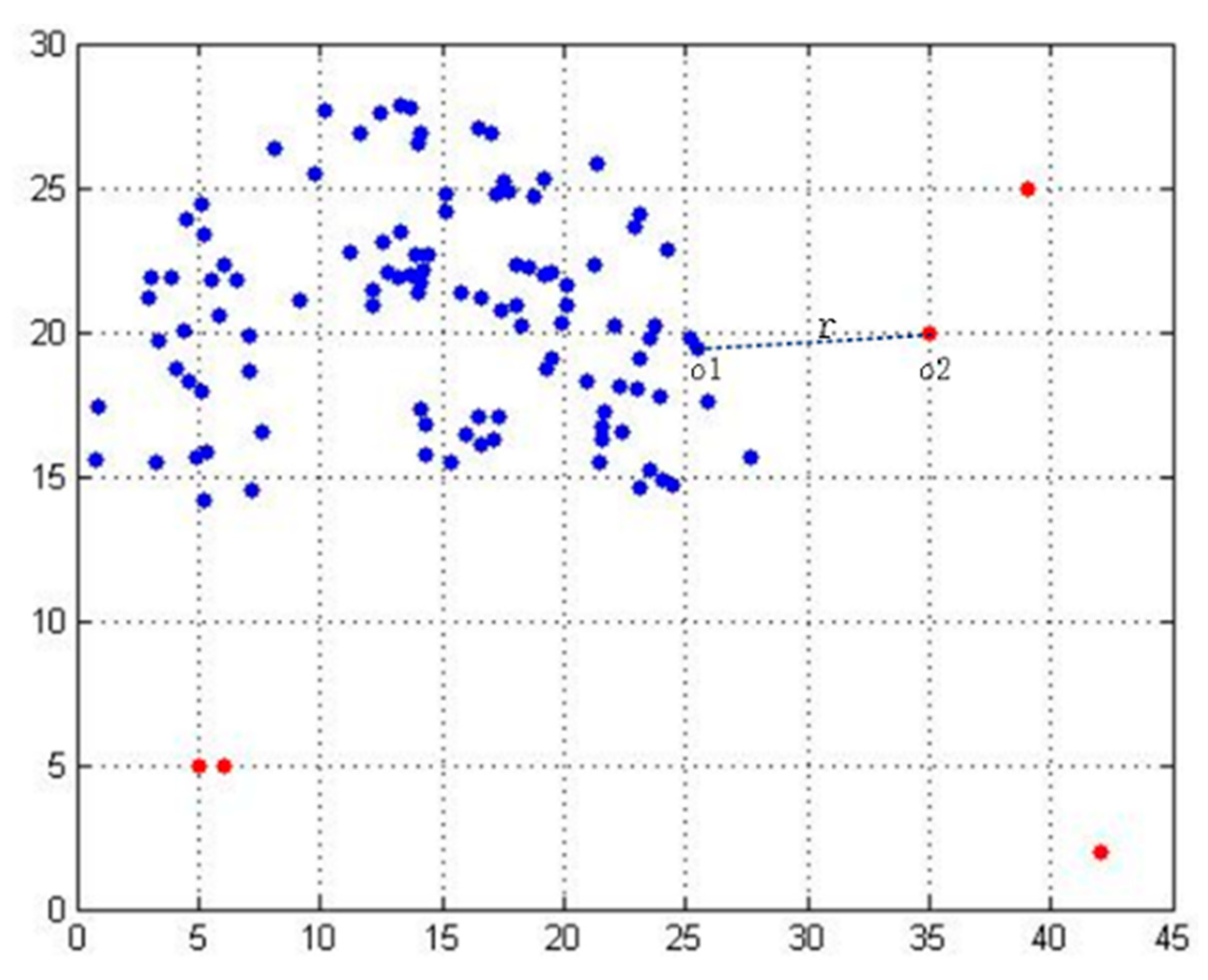
Outlier detection is an important aspect of data mining. The commonly used outlier detection methods are distance-based and density-based outlier detection methods, and their improved methods. These methods are based on the concept of nearest neighbor, so the nearest neighbor selection is very important for outlier detection. As shown in
Figure 5, when the nearest neighbor k of data point o1 is small, the cluster that should be a cluster is divided into several data clusters, which results in the neglect of some neighborhood relationships that should exist. The representation of this situation in the nearest neighborhood graph is that the original whole connected subgraph is split into many small connected subgraphs, and then the data points with the same properties are misclassified into different clusters to get the wrong data relations. Similarly, if we set the nearest neighbor value larger, it will have an overall impact, so that the dataset itself is not a cluster that is divided into a data cluster. Secondly, on the whole, o2 is an outlier, but when the nearest neighbor of o1 is r, the outlier o2 is the nearest neighbor of the data point o1.
The nearest neighbor can reflect the relationship between data points, and one form of this relationship is the neighborhood graph, which can be constructed by connecting each data point to its nearest neighbor [
25]. However, it is difficult to identify outliers accurately only through the single concept of nearest neighbor, so the concept of mutual neighbor is introduced. The mutual neighbor graph can be constructed by connecting the mutual neighbors of each data point.
Definition 8. Nearest neighbor search method. For a given dataset X and the data point q to be queried. The goal of the nearest neighbor search is to find a subset of Formula (1) in dataset X. Definition 9. Mutual neighbor (MN). If p is the neighbor of q and q is the neighbor of p, then we call p and q mutual neighbors.
Definition 10. Mutual neighbor graphs. The graph constructed by connecting each point to its mutual neighbor is called a mutual neighbor graph.
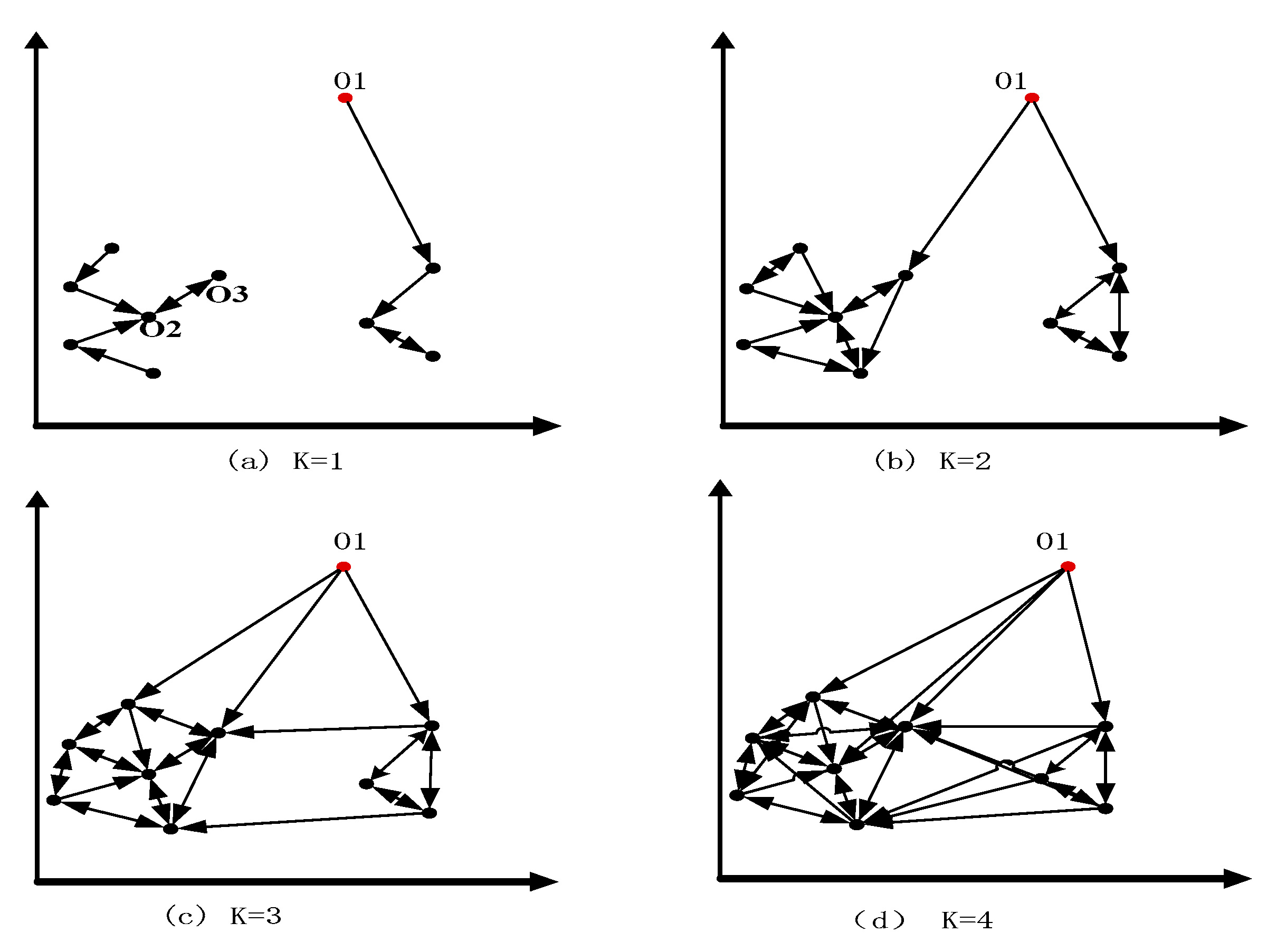
As shown in
Figure 6, the mutual neighborhood graph consists of data points. Firstly, the first nearest neighbor of each data point is searched, and the arrow points to the nearest neighbor direction of the data point, and the nearest neighbor of each data point is obtained, at the same time, the mutual neighbor points are obtained. As shown in
Figure 6a, O2 is the nearest neighbor of O3 and O3 is the nearest neighbor of O2, so O2 and O3 are mutual neighbors. Similarly, continuing to search for the second nearest neighbor of each data point, and getting the nearest neighbor and mutual neighbor of each data point. As shown in
Figure 6b, the point without mutual neighbors is only O1. Then, we look for the third nearest neighbor of the data point, as shown in
Figure 6c. At this point, there is still only O1 without mutual neighbors. When the nearest neighbors k = 2 and k = 3, the number of points without mutual neighbors is the same, and they are only O1 points, so the mutual neighbor graph of the whole dataset remains stable and the algorithm ends. As the number of nearest neighbors increases gradually, the number of mutual neighbors of normal data points increases correspondingly, so that the mutual neighbor graph becomes more and more complex, and the outliers remain unchanged. Based on the above description, we can judge the abnormal situation of data points in the dataset by observing the changes of the mutual neighbor graph of data points.
As the mutual neighbor graph is a form of a data neighbor graph, for many datasets with complex distribution, it cannot be measured accurately through a mutual neighbor graph intuitively, so we propose the concept of the number of residual neighbors in this paper. With the gradual increase of the nearest neighbor k, the number of mutual neighbors of data points is constantly changing; meanwhile, the number of data points without mutual neighbors is also changing. To make outlier detection more intuitive and effective, we can judge the outliers by observing the change of the number of residual neighbors.
Definition 11. The number of residual neighbors. If the data points p and q are mutual neighbors, the number of data points without such a mutual neighborhood is the number of residual neighbors.
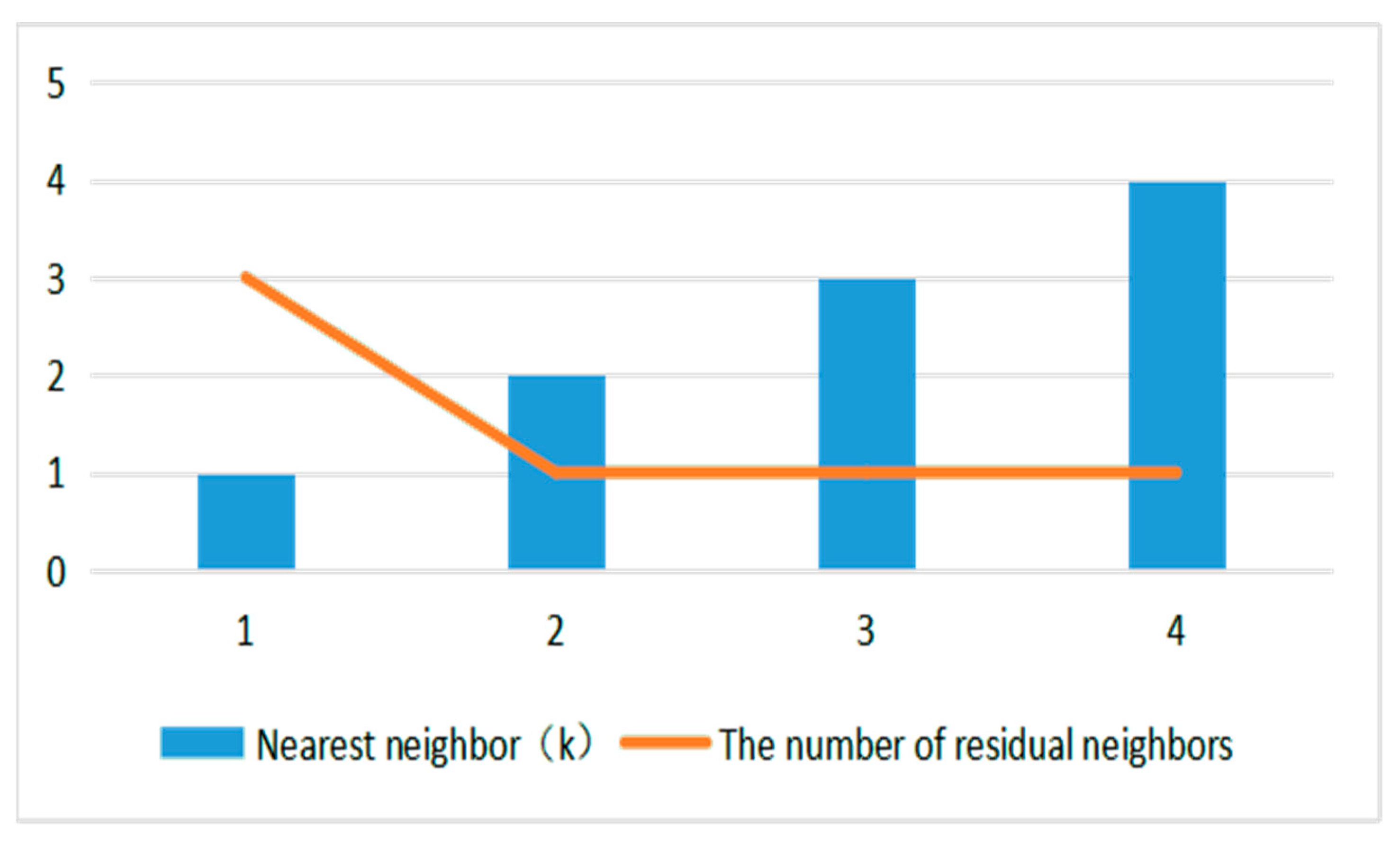
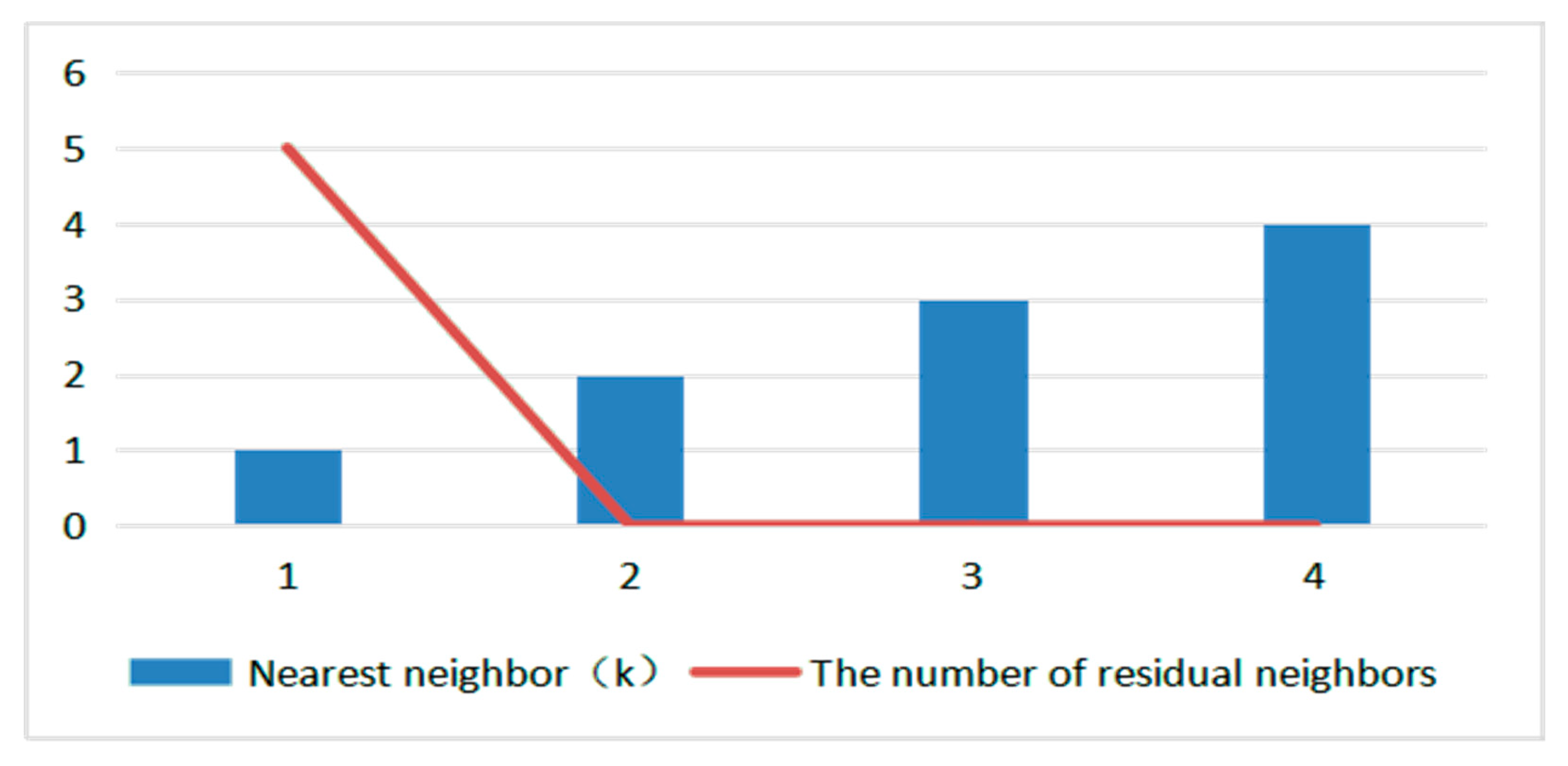
As shown in
Figure 7, it is a variation curve of the number of residual neighbors of the data point in
Figure 6. It can be seen intuitively that when k = 2 and k = 3, the number of residual neighbors is equal, and the number of residual neighbors in the dataset is 1, which satisfies the termination condition of the algorithm. Therefore, it is considered that the whole neighborhood is stable and the algorithm is terminated. So, for the dataset shown in
Figure 6, O1 is the outlier obtained by the parameter-free outlier detection algorithm.
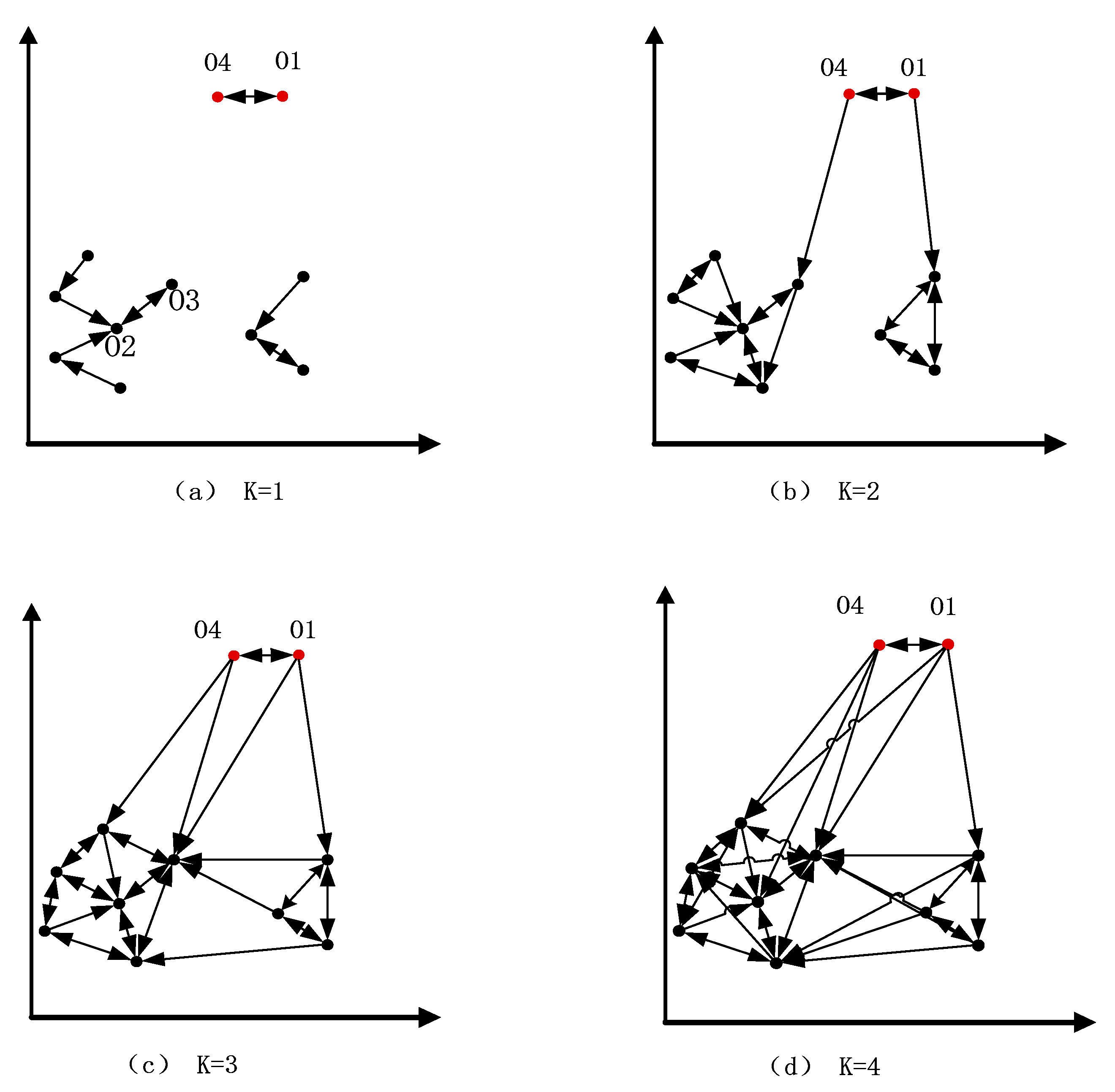
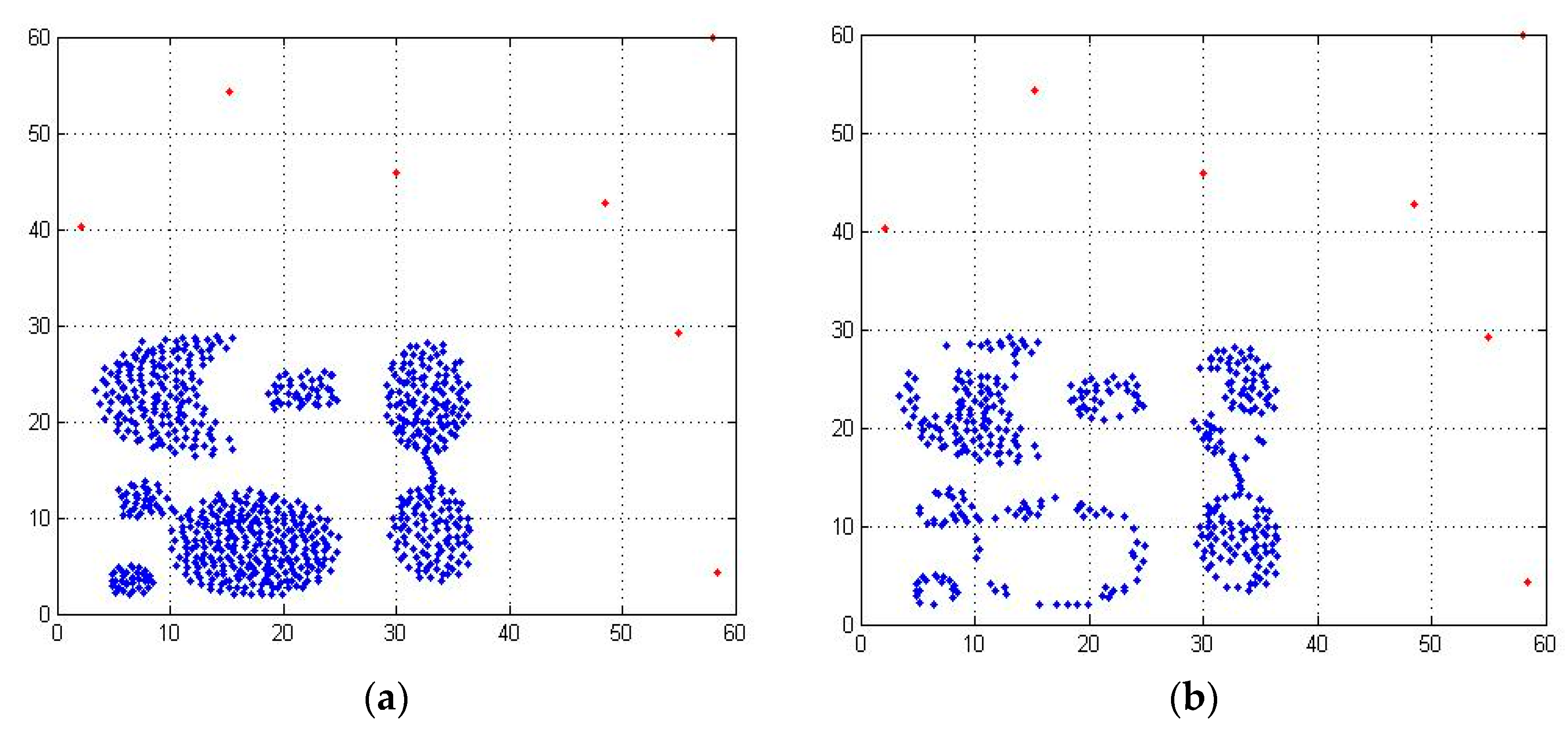
In some distributions of data, outliers exist not only in the form of single points but also in the form of outliers. As shown in
Figure 8, O1 and O4 are outliers and the rest are normal points. Firstly, as the number of nearest neighbors increases gradually, the mutual neighbor graphs of dense clusters become more and more complex until they are stable (only k = 1–4 mutual neighbor graphs are listed in this paper). Secondly, we get the number of residual neighbors as shown in
Figure 9. When k = 2 and k = 3, the number of residual neighbors is equal, and the number of residual neighbors in the dataset is 0, which satisfies the termination condition of the algorithm, but the outliers O1 and O4 of the algorithm cannot be detected correctly.
Therefore, in order to improve the accuracy of the algorithm, when the relationship between data clusters is stable, we compare the size of each data cluster and the number of nearest neighbors. If the size of the cluster is smaller than the number of nearest neighbors, it means that the data cluster is an anomalous cluster, so we can obtain a more accurate set of outliers.
Based on the concept of the number of residual neighbors, Algorithm 2 is used to describe the process of parameter-free outlier detection. In Algorithm 2, we first input the initialized dataset. As the number of nearest neighbors k increases gradually, we traverse to calculate the number of mutual neighbors and residual neighbors until the number of residual neighbors does not change. Then, a single outlier is obtained. By comparing the size of the data cluster with the nearest neighbor k, we get the outlier cluster and the outlier set as follows:
| Algorithm 2. Parameter-free outlier detection |
| Input: Candidate dataset |
| Output: Outlier Dataset |
| Constructing the Mutual Neighbor Graph G; k; C1; |
| k = 1; |
| (1)Random an object x; visited(x) = true; |
| while y∈G ∪ visited(y)! = true |
| then visited(y) = true; calculate (y, mutual neighbor); |
| Calculate (y, single neighbor, num) |
| k = 2; go to(1); |
| k = 3; go to(1); |
| …… |
| if num then outlier = true; |
| if(C1<k) |
| then outlier = true |
There are several characteristics of data distribution in outlier detection: the number of normal data points is large and dense, the number of abnormal data points is small and sparse, and the number of nearest neighbors is uncertain. Firstly, we study the shortcomings of the existing outlier detection algorithms, then combine the above data distribution characteristics, and finally propose the parameter-free outlier detection algorithm in our paper. The algorithm realizes the function of detecting more reasonable outliers efficiently without human participation.


