Article

A Novel Approach to Component Assembly Inspection Based on Mask R-CNN and Support Vector Machines

1
Key Laboratory of Advanced Manufacturing Technology, Ministry of Education, Guizhou University, Guiyang 550025, China
2
Department of Industrial Engineering and Management, Yuan Ze University, Taoyuan 32003, Taiwan
*
Author to whom correspondence should be addressed.
Information 2019, 10(9), 282; https://doi.org/10.3390/info10090282
Submission received: 26 July 2019 / Revised: 20 August 2019 / Accepted: 28 August 2019 / Published: 11 September 2019
(This article belongs to the Special Issue IoT Applications and Industry 4.0)

Abstract

:
Assembly is a very important manufacturing process in the age of Industry 4.0. Aimed at the problems of part identification and assembly inspection in industrial production, this paper proposes a method of assembly inspection based on machine vision and a deep neural network. First, the image acquisition platform is built to collect the part and assembly images. We use the Mask R-CNN model to identify and segment the shape from each part image, and to obtain the part category and position coordinates in the image. Then, according to the image segmentation results, the area, perimeter, circularity, and Hu invariant moment of the contour are extracted to form the feature vector. Finally, the SVM classification model is constructed to identify the assembly defects, with a classification accuracy rate of over 86.5%. The accuracy of the method is verified by constructing an experimental platform. The results show that the method effectively completes the identification of missing and misaligned parts in the assembly, and has good robustness.

1. Introduction

Assembly is a very important process in manufacturing [1]. A large number of mechanical components can be involved in the process. It is hard to prevent machines from having faults related to missing parts and misalignments. These faults in the assembly machines can cause high production downtime and increase running costs [2,3]. Due to rising labor and facility costs, automation and accuracy in assembly have become the clear solution [4]. The use of computer vision systems for assembly inspection has seen a dramatic increase in recent years. Automated assembly machines operate continuously to achieve high production rates [5]. Computer vision technology has been used to provide product inspection, which helps decision making in production systems [6].
Computer vision-based inspection has become one of the most important application areas [7]. Many researchers, from different fields, have studied and developed various inspection methods with different applications. Andres et al. presented the development of a machine vision inspection system (MVIS) purposely for car seat frames, as an alternative to human inspection [8].
They optimized the techniques for visual inspection through qualitative analysis and the simulation of human tolerance for inspecting car seat frames. Jiang et al. [9] designed a machine vision inspection system connected with an MCU to perform the surface detection of shaft parts. Their experiment showed that no defect was omitted, and the false alarm error rate was less than 5% and met the demand for shaft part on-line real-time detection. Wu et al. [10] proposed a novel, accurate subpixel edge detection algorithm for a thin sheet part, based on machine vision. The experimental results indicated that the inspection accuracy of this algorithm was high, with the subpixel edge location accuracy reaching the micrometer level. The traditional machine vision detection method is to extract image features and construct a classifier to complete target detection. The most effective features for image classification include shape, intensity, geometry, gradient, and texture. Common classifiers include the Support Vector Machine, Adaboost, Random Forest, etc. [11,12,13]. For example, Bohlool et al. [14] presented a cost-efficient automated visual inspection (AVI) system utilized as a quality control system. The scale invariant feature transform (SIFT) was used to acquire good accuracy and make it applicable in different situations, with different sample sizes, positions, and illuminations. Sachin et al. [15] proposed an algorithm to accomplish object recognition by using two different methods in which the classification of the extracted features of the object image is based on artificial neural networks (ANN) and SIFT-based features, using Euclidean distance measurements and a measurement algorithm to match the extracted features of the object image to complete image recognition. Chuahan et al. [4] proposed three MVIS methods based on computer vision techniques. The first method was based on Gaussian mixture models (GMMs), the second method used an optical flow approach, and the third method was based on running average and morphological image processing operations. They developed a machine vision performance index (MVPI) for the following measures of performance: accuracy, processing time, speed of response, and robustness against noise. Jiang et al. [9] proposed a method to detect the shaft part surface. They used the dark-field and forward illumination technology to acquire images with a high contrast: First, the images were segmented into bi-value images; then, the main contours were extracted; next, the coordinates of the center of gravity of the defect areas were calculated, that is, the point coordinates were located; finally, the locations of the defect areas were marked by the coding pen in communication with the MCU.
In recent years, deep learning has won numerous contests in pattern recognition. Convolutional neural networks (CNNs) show excellent performance for image processing [16,17]. In 2012, a CNN approach achieved the best results for ImageNet classification [18]. On the basis of CNN, Girshick proposed the R-CNN algorithm based on the candidate region [19]. R-CNN uses the selection search (selective search) algorithm to obtain possible targets in the candidate region, and has achieved good effects [20]. In order to improve the detection accuracy and speed of R-CNN, some excellent algorithms have been proposed in recent years, such as Faster R-CNN, YOLO, and Mask R-CNN [21,22,23]. So far, deep learning has been widely used in industrial production and has achieved good results.
This paper presents a method based on Mask R-CNN and Support Vector Machine (SVM) that uses the Mask R-CNN segment assembly image to extract feature vectors for classification. This method meets the requirements of industrial production. The results show that our method can efficiently identify the missing part and misalignment assembly problems in production.

2. Research Method

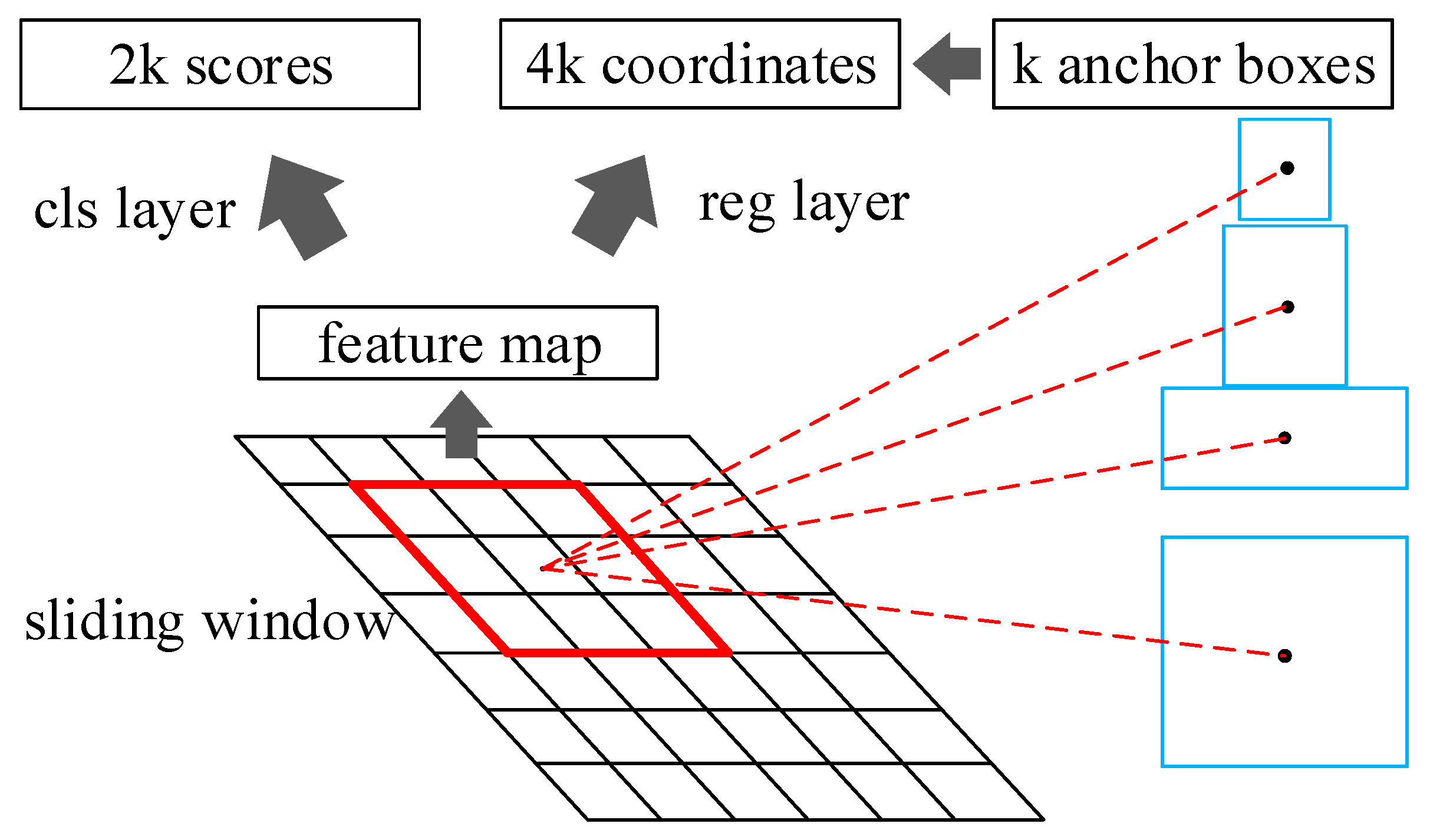
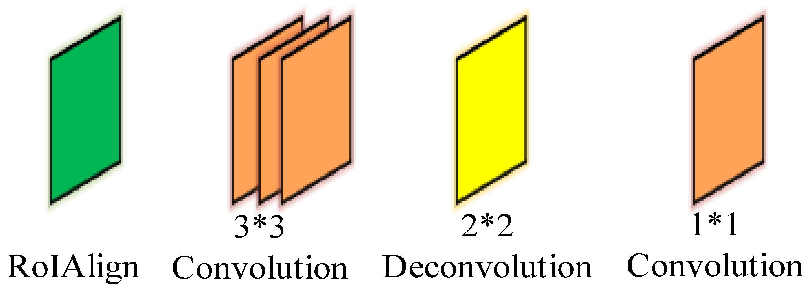
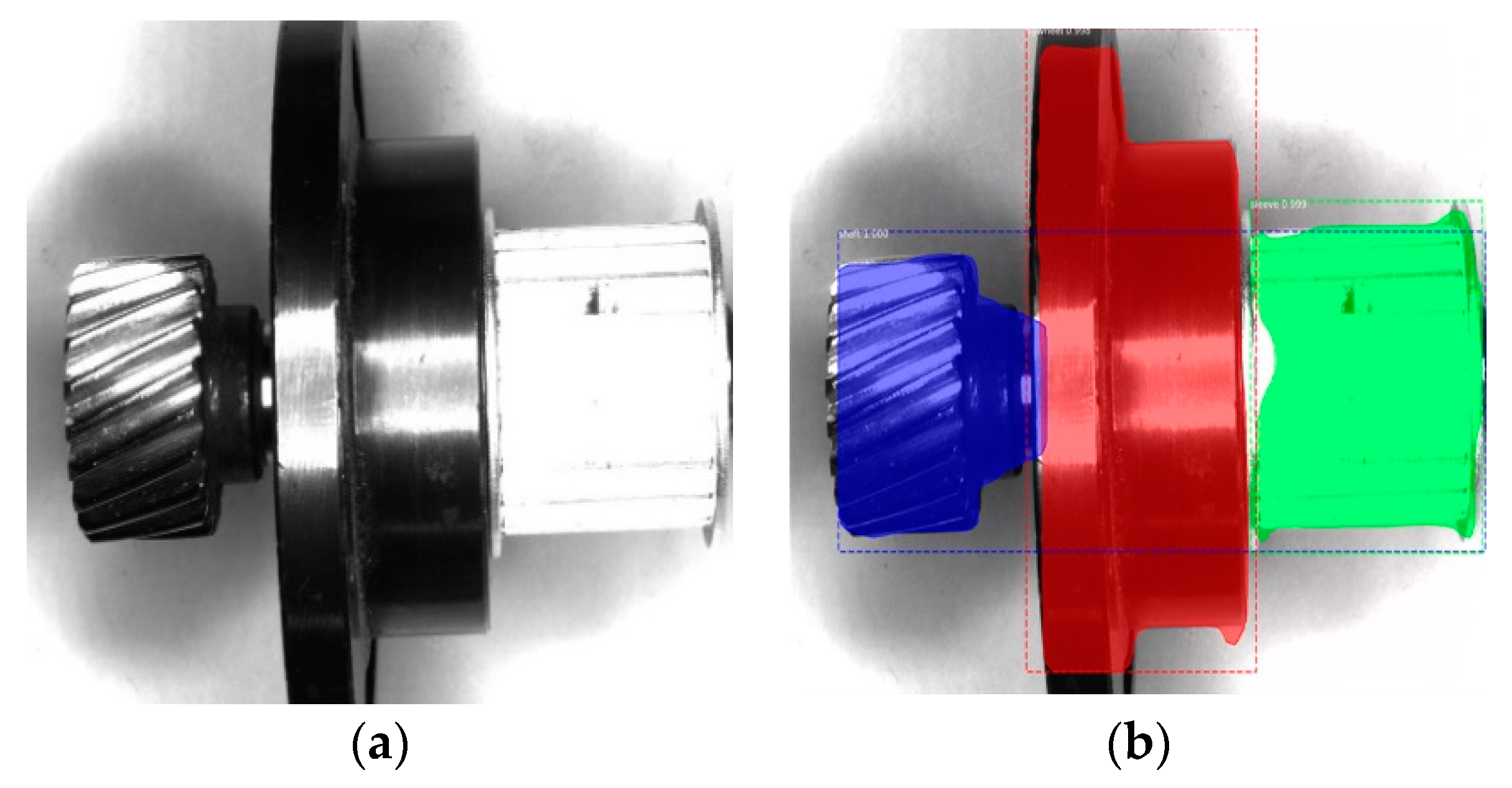
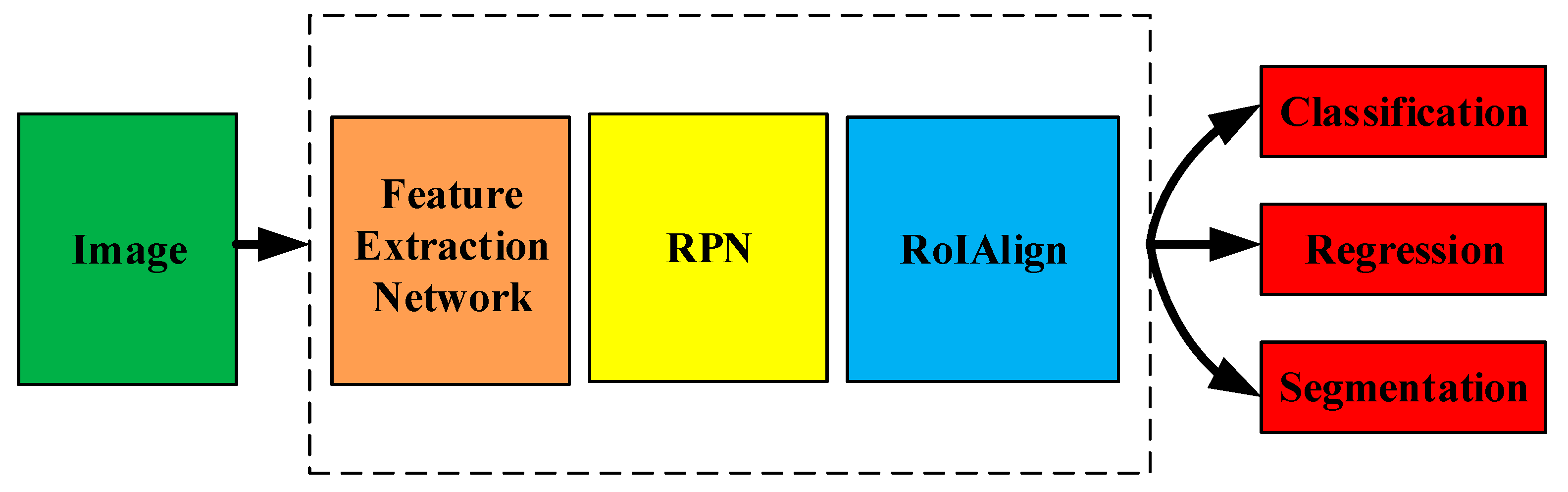
2.1. Instance Segmentation Based on Mask R-CNN

Traditional visual detection methods rely on manual selection for image segmentation. The selection of the artificial method determines the quality of the segmentation effect; for example, OTUS is a traditional image segmentation method. In this paper, the deep learning method was selected for image segmentation. Thus, the errors caused by the manual selection of features and methods were avoided. We used the Mask R-CNN model to recognize and segment the part image and obtain the outline of the assembly. Then, the feature vectors of the contour images were extracted and sent to Support Vector Machines for training to identify the defects of various assembly types. The algorithm flow is shown in Figure 1.
Mask R-CNN is an instance segmentation algorithm that was first proposed by Kaiming He. It is a deep neural network model developed on the basis of Faster R-CNN. Its main functions are target detection, target classification, and target segmentation. The Mask R-CNN model adds a mask segmentation part based on Faster R-CNN, and changes ROIPooling to ROIAlign for better detection. Mask R-CNN is composed of four parts: the feature extraction network, the region proposal network (RPN), ROIAlign, and the target recognition segmentation network. The structure of Mask R-CNN is shown in Figure 2.
The feature extraction network is the backbone network of Mask R-CNN, which can use VGG16, GoogleNet, ResNet101, and other networks [24,25]. The backbone network in this article uses the ResNet101 network. The basic structure of the ResNet network is the residual module, which can solve the problem of gradient dispersion with the increase in network model depth to a certain extent. It improves the network performance, and has better performance in multi-category recognition. The FPN network used in this paper combines feature maps of different depths, with the generated feature map containing better semantic information [26]. Using ResNet101 as an example, starting with five different depth feature maps, which are respectively recorded as C1, C2, C3, C 4, and C5, the FPN network recombines the five different depth feature maps to generate new feature maps: P2, P3, P4, P5, and P6. For i = 1, 2, 3, 4, 5, and 6; correspondence is shown in Equation (1).
P i = c o n v ( s u m ( u p s a m p l e ( P i + 1 ) , c o n v ( C i ) ) ) P 5 = c o n v ( c o n v ( C 5 ) ) P 6 = d o w n s a m p l e ( P 5 )
where conv () is the convolution operation, sum () is the summation operation, upsample () is the upsampling operation, and the downsample () is the downsampling operation.
The RPN is a full convolutional network (FCN) that can quickly generate high-quality candidate boxes with different ratios. The center of each box is called an anchor, which divides the image into multiple regions of interest. The RPN performs a convolution operation on the feature map through a sliding window, and maps the sliding window to a low-dimensional vector. The RPN structure is shown in Figure 3.
After generating the anchor, according to the value of RPN network regression, the anchor is modified to better adapt to the object. The correction value of the anchor box includes Δx, Δy, Δh, and Δw. The correction calculation is as shown in Equation (2).
{ x = ( 1 + Δ x ) · x y = ( 1 + Δ y ) · y w = exp ( Δ w ) · w h = exp ( Δ h ) · h
where Δx, Δy, Δh, and Δw are the correction values of the anchor; x, y represent the central coordinates of the anchor; and w, h represent the width and height of the anchor.
In this paper, the region proposal network uses a 3 × 3 convolution kernel to slide on the feature map, and generate a 256-dimensional vector with each sliding operation. The vector is input into two full-connection layers to classify the regression. Each sliding window center generates an anchor of five lengths and three widths.
In the sample selection strategy, non-maximum suppression (NMS) is used to select samples. Interview over Union (IoU) is the ratio of the intersection area of the detection result and the area of the ground truth. It is shown in Figure 4.
The calculation is shown in Equation (3). IoU is used on a discriminating basis to distinguish whether the target is included in the anchor. Samples were selected for training according to a 1:1 ratio of positive and negative samples.
I o U = D e t e c t i o n   R e s u l t G r o u n d   T r u t h D e t e c t i o n   R e s u l t G r o u n d   T r u t h
In the next stage, the size of the anchor needs to be adjusted to a fixed size. To address the misalignment, Mask R-CNN applies a simple, quantization-free layer named RoIAlign, which is able to faithfully preserve the precise positions. The feature aggregation method of ROI Pooling is used in Faster R-CNN, and there are two quantization operations in this process. First, from the original image through the convolution network to the feature map, the position of the region proposals frame is obtained, which may have floating-point numbers; the rounded operation causes this first quantization. Secondly, when ROI Pooling finds the position of each small grid; this may involve cases where the floating-point number is rounded. The results of these two quantifications cause the position of the region proposals frame to deviate. This paper’s algorithm uses the RoI Align method to convert the feature map into a fixed-size feature map. The RoI Align method uses bilinear interpolation to obtain pixel values at coordinates of floating-point pixels. The back-propagation calculation of RoI Align is as shown in Equation (4):
L x i = r j [ d ( i , i * ( i , j ) ) < 1 ] ( 1 Δ h ) ( 1 Δ w ) L y r j ,
where xi is the pixel point on the feature map before pooling, yij represents the j-th point of the i-th candidate area after pooling, i*(i, j) represents the source of the pixel yij, d(,) represents the distance between two points, and Δh and Δw represent the difference between the xi and x i*(i,j) horizontal and vertical coordinates.
The fixed-size feature map is sent to the functional network known as the head for calculation. The Mask R-CNN is the optimization of Faster R-CNN. There are three branches that contain the information to predict: reg-layer, cls-layer, and object mask. The first two branches are used for bounding-box classification and regression. They use the fully connected layer and the SoftMax layer and complete the classification and position box regression. In order to get more accurate shape information, the third branch is used to the output object mask. Mask R-CNN adds a branch for the forecast mask based on the Faster R-CNN, which uses an FCN structure. FCN is an end-to-end upsampling algorithm; there is no fully connected layer at the end that needs a fixed size of activations. The structure of FCN is shown in Figure 5.
According to the feature of the part, there are four convolution operations on the 14 × 14 feature map generated by RoI Align. The convolution kernel size is 3 × 3, and the feature image size is 14 × 14. Then, the size is upsampled to 28 × 28 by a 2 × 2 deconvolution layer with a convolution kernel. Finally, a 1 × 1 convolution layer and a sigmoid activation layer are used to obtain a 28 × 28 binary feature image. The object is segmented from the background to get the exact shape. As a result of the mask layer being added, the loss function is defined as in Equation (5):
L o s s = L o s s c l s + L o s s r e g + L o s s m a s k
where Losscls is classification loss function, Lossreg is regression loss function, and Lossmask is mask regression function.

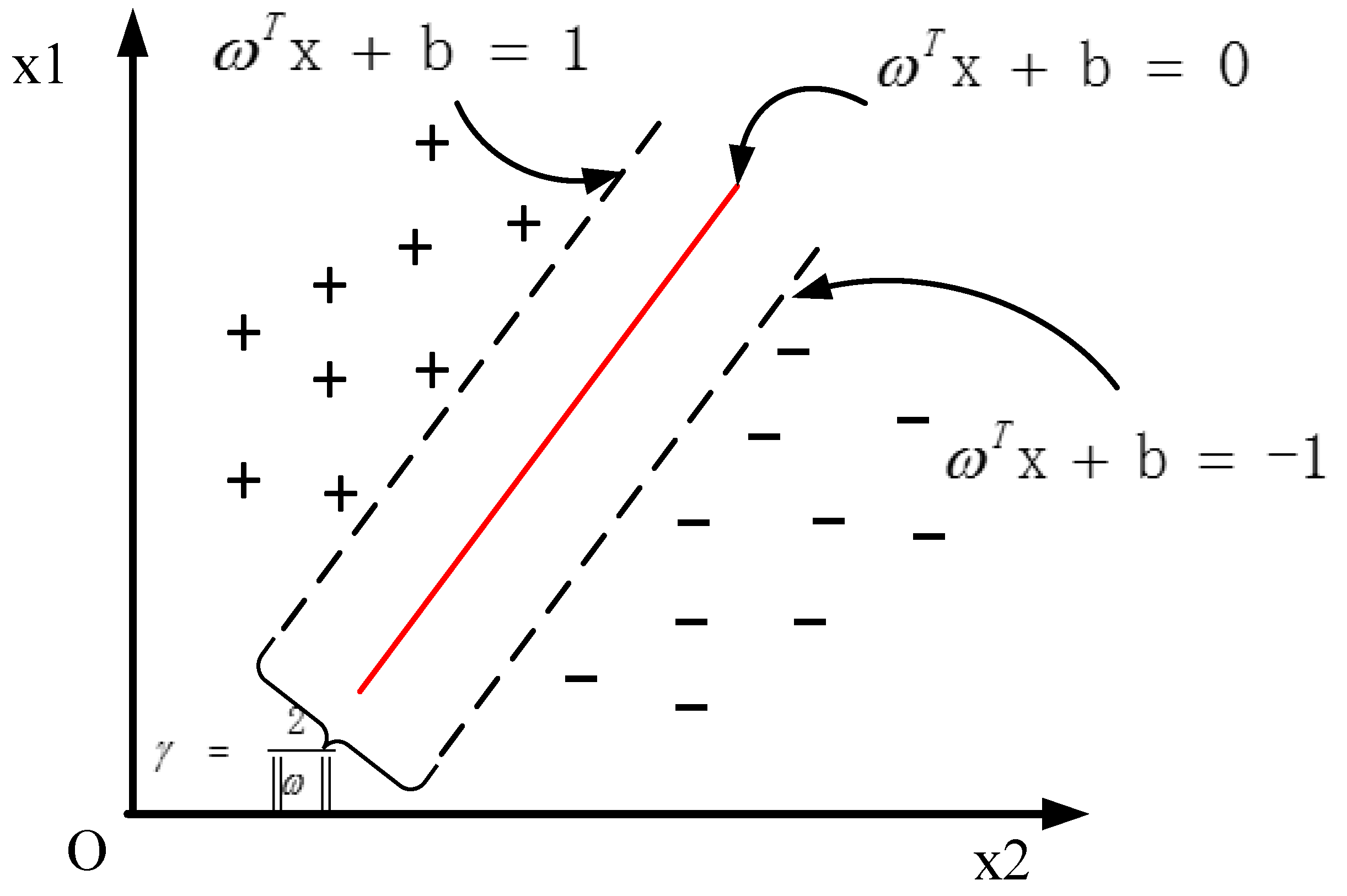
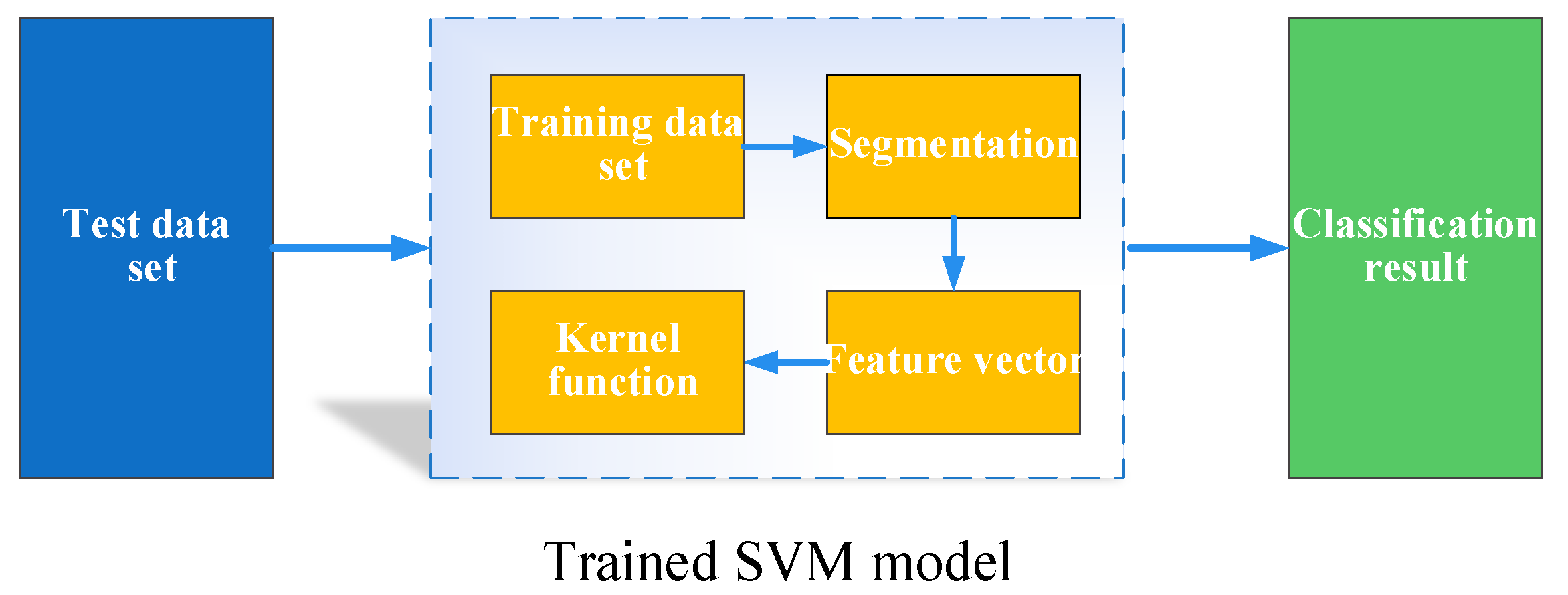
2.2. Component Assembly Inspection Based on SVM

The support vector machine is based on the theory of statistical learning. It has the advantages of global optimization and generalization ability, and performs well and has unique advantages in solving small sample, nonlinear, and high-dimensional pattern recognition problems. The principle of the Support Vector Machine is shown in Figure 6.
The first consideration of SVM is the problem of two classifications. For a given sample set D, as shown in Equation (6),
D = { ( x 1 , y 1 ) , ( x 2 , y 2 ) , ( x m , y m ) } ,   y { 1 , + 1 } ,
we can find a hyperplane, which is expressed as:
ω x + b = 0 ,
where ω is the weight vector, and b is biased. ω and b determine this hyperplane. The hyperplane can correctly classify the sample into two categories, and any of the sample spaces (xi, yi) ∈ D. We get Equation (8):
ω x i + b 0 ,   y i = 1 ω x i + b 0 ,   y i = 1 s . t .   y i ( ω x i + b ) 1 .
ω, b in Equation (9) determine this optimal hyperplane, and y represents the category label. In order to maximize the interval, it is necessary to solve the optimal hyperplane:
min Φ ( ω ) = ω 2 / 2 s . t .   y i ( ω x i + b ) 1 ,   i = 1 , 2 , 3 .
From the above, we get the Hard-Margin Support Vector Machine model. In order to solve the minimum value of the above function, the Lagrangian multiplier method is introduced to obtain its dual problem, and Equation (10) is linearly transformed into:
min W ( α ) = i = 1 l α i 1 2 i = 1 l j = 1 l α i α j y i y j < x i · x j > s . t .   i = 1 m α i y i   = 0 α i 0 ,   i = 1 , 2 , 3 , , m .
where αi represents the Lagrange multiplier. The Lagrange multiplier method was used to transform the problem into a quadratic programming problem and obtain a classification model; the function is as follows:
f ( x ) = sgn ( α i y i ( x x i ) + b ) .
For the linearly inseparable problem, the data can be mapped to a higher feature space by a kernel function, which is transformed into a linearly separable problem. Here, K(x, xj) is a kernel function, and common kernel functions are linear kernel functions, Gaussian kernel functions, etc. We build a Support Vector Machine by choosing the appropriate kernel function and penalty coefficient.
In order to ensure the accuracy of detection, the one-against-one multi-classification algorithm is selected to improve the detection accuracy. The commonly used kernel functions are shown in Table 1.

3. Data Preparation and Training

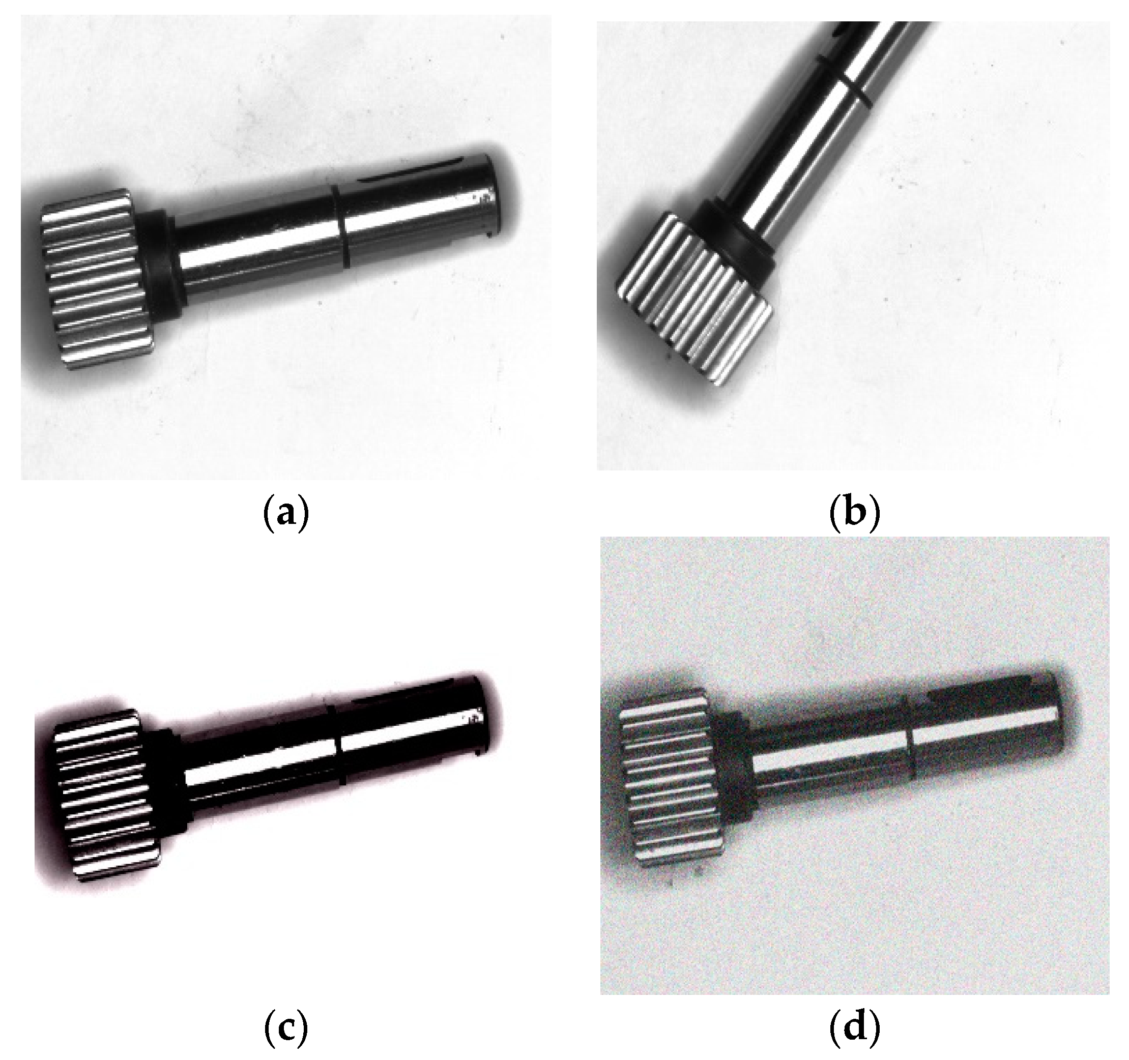
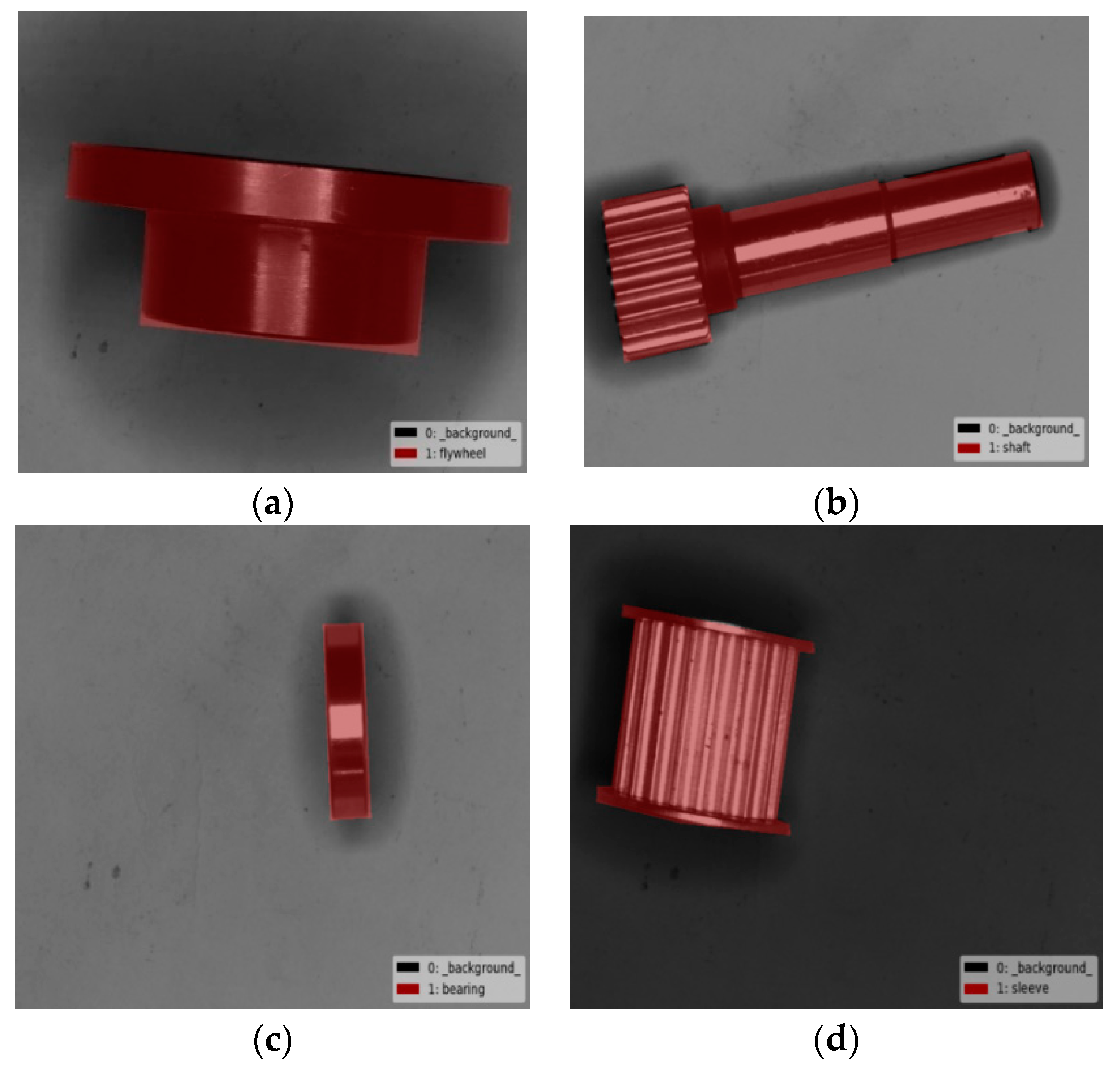
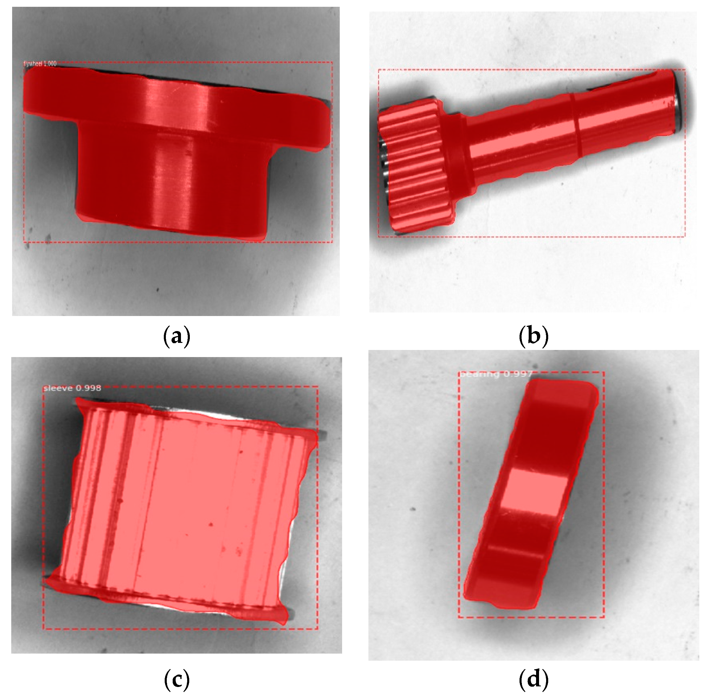
3.1. Data Preparation

We collected the images by building a part image acquisition platform, as shown in Figure 7. The part image acquisition system consists of a conveyor, an industrial CCD camera, a lens, an image acquisition card, a light-emitting diode (LED) curved light source, and a computer. Before the collection, the lens focal length and the position of the light source needed to be adjusted to ensure the image acquisition quality. These images include four categories: the flywheel, the bearing, the sleeve, and the shaft. We collected a total of 600 images. Images being too large causes exponential growth in the number of deep neural network parameters. The image size we collected was 256 × 256.
As a result of the small number of samples in the collection, it was easy to cause overfitting during model training. In order to reduce the risk of overfitting, the data enhancement method was used to extend the collected dataset. Common methods for the data enhancement of image samples are random trimming, translational transformation, scale transformation, image rotation translation, contrast transformation, noise disturbance, color jitter, etc. The methods of data enhancement in this paper are to randomly crop the image, change the image contrast, and add noise; some examples are shown in Figure 8. We selected some training set images for data enhancement. After enhancement, the number of images in each class was 250, and the image size was 256 × 256. The ratio of the training set, validation set, and test set was 8:1:1. Detailed information about the datasets is given in Table 2.
The LabelMe software was used to mark the training samples for the enhanced data. The marked files automatically added the background and assigned the background to a class. This generates the corresponding folder containing the image information. The model automatically reads the relevant information in the folder for training. An example of annotated training images are shown in Figure 9.
In order to get a more stable and robust model, the labeled training samples were divided into K-fold cross-validation (here, K = 5). The initial sample set is divided into five sub-samples and numbered separately. One of the sub-samples was used as the data for the verification model, and the other samples were used for training. Cross-validation was performed five times, and each sub-sample was verified once.

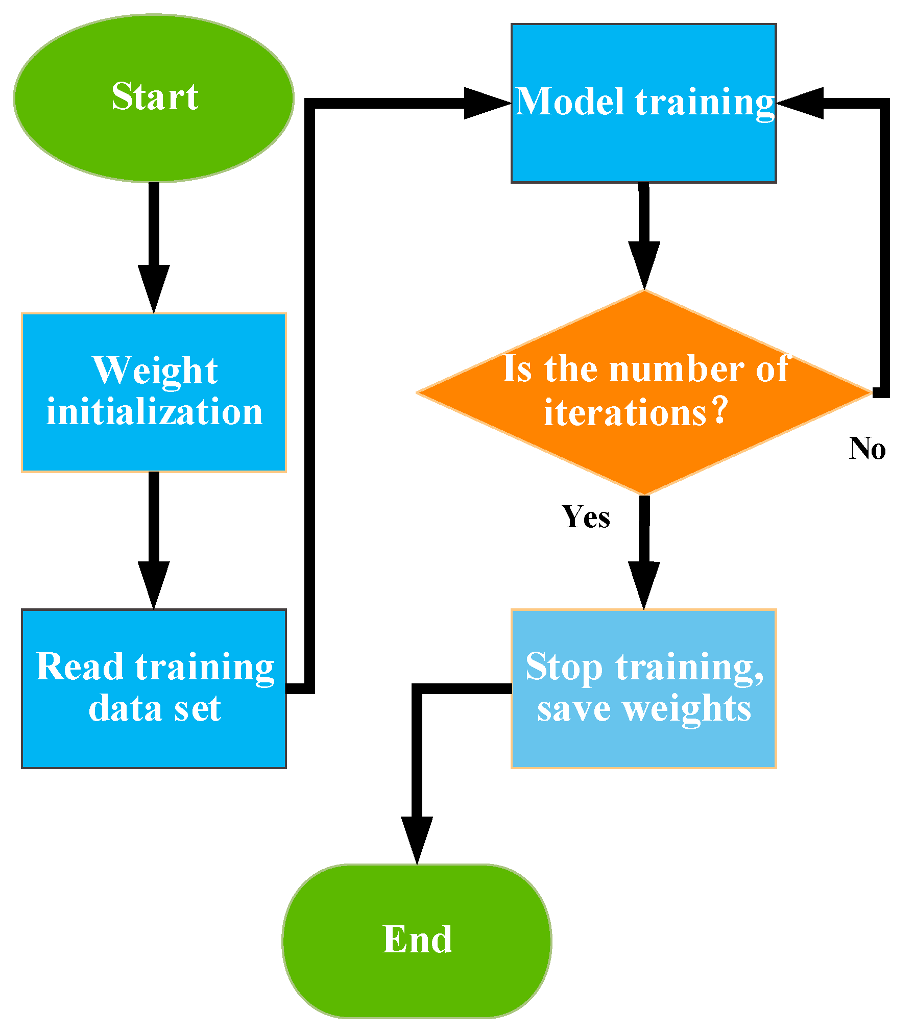
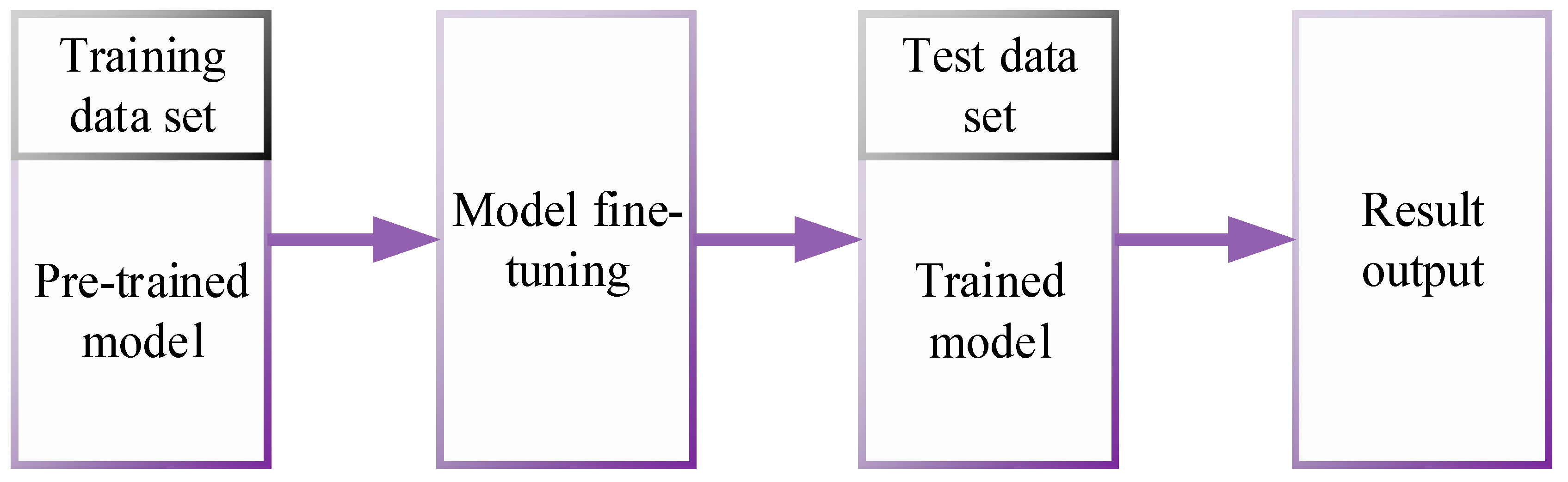
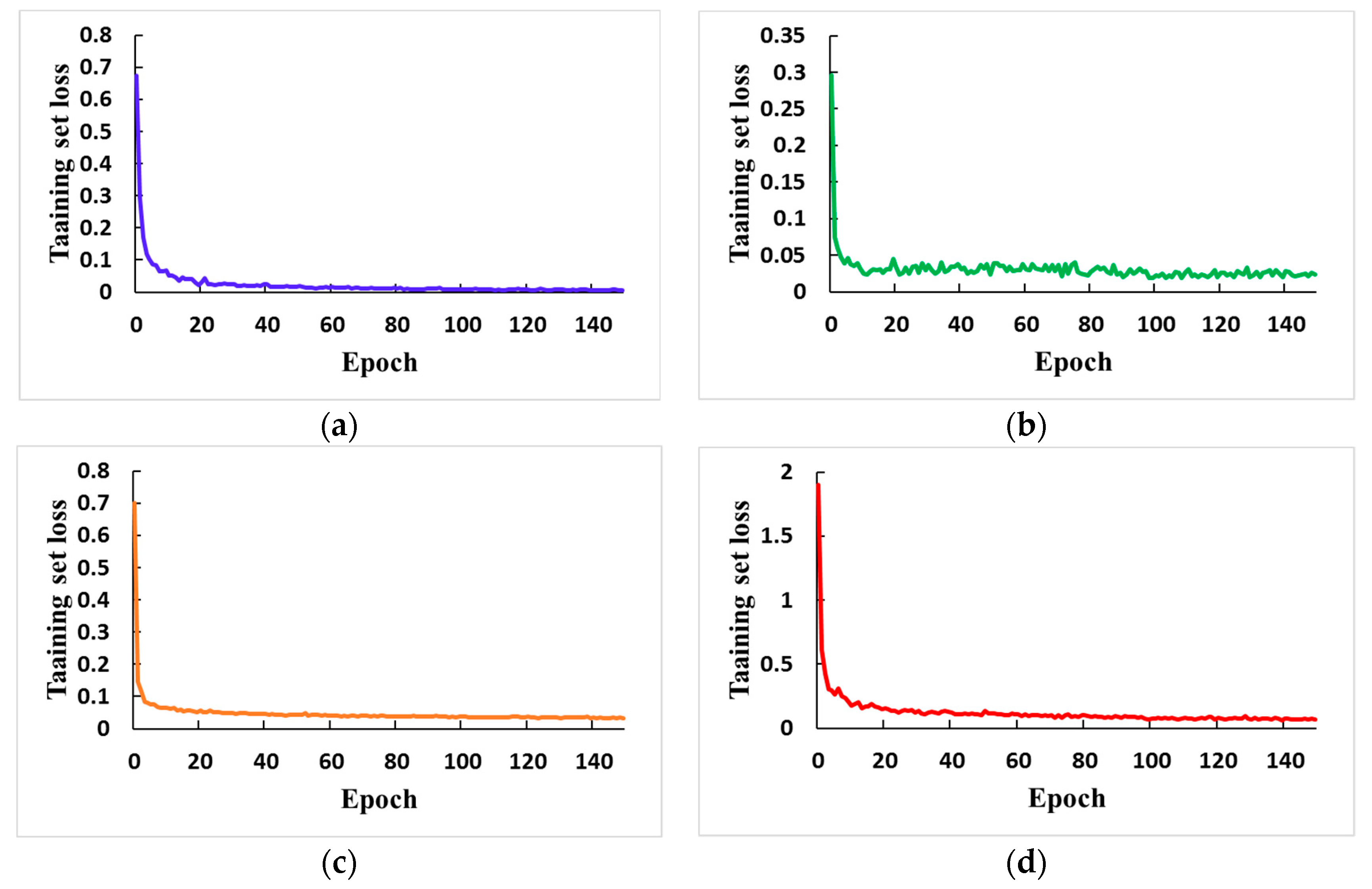
3.2. Training Methods and Details

The deep network model requires a large amount of tag training data to prevent the network from overfitting. The labeling steps of the dataset are very complicated. Therefore, in this study, we trained the training set by means of transfer learning. It uses the trained model to initialize the network, and shares the same features in the model. We used new data samples to train the special classification network parameters. The trained model was able to achieve the desired effect. Using transfer learning can speed up network convergence, reduce computational strength, and solve the problem of underfitting caused by the lack of sufficient tag training data. In this study, according to the characteristics of the part image, the trained model was fine-tuned using a large amount of our own dataset. The hyper-parameters were set to achieve better training results. The parameter fine-tuning process used in the training is shown in Figure 10.
The iteration and epoch were set during the training process, and the loss function value was recorded after each iteration of one epoch. The entire model training process is shown in Figure 11.
Mask R-CNN was implemented on Python 3, TensorFlow, and Keras. We used the ResNet101 backbone to obtain higher accuracy. As the network depth and the size of datasets increase, the use of GPU to train deep neural networks takes less time. We used the GPU to train the Mask R-CNN. The maximum number of iterations for the model parameters was 150 epochs with a momentum of 0.9. The learning rate was set to 0.001, which is more suitable for a small batch size with a faster convergence, and the weight decay was set to 0.0001. An RoI was defined as positive when it had an IoU with a ground-truth box more than 0.5; otherwise, it was deemed as negative. The ratio of positive to negative was 1:1. The RPN anchor spanned five scales: 8, 32, 64, 128, and 256; and three ratios: 0.5, 1, 2. We set the mini-batch as two images on one GPU.
In the SVM training, we adopted the one-against-one method, and reduced its computation to a great degree. We trained the Support Vector Machine model with the training dataset. In the training process, we used different kernel functions to achieve better results. The training process is shown in Figure 12.

4. Experimental Results and Analysis

The loss function value of the model gradually decreases with the increase in the number of iterations, and tends to be stable. The value of the loss function is shown in Figure 13.
After the model was trained, we selected the test set for testing. We selected a single part to test; the test results are shown in Figure 14. The red part of the figure is the result of the example segmentation of the part, which can accurately segment the shape of the target in the image, generate the corresponding segmentation mask, and display the outline of the part. The text indicates the name of the category, the number indicates how well the part matches the category, and the box indicates the position of the part in the image. As a result of the powerful generalization ability of the model, the model shows better robustness to images with different brightness and different directions.
The model detects the assemblies containing multiple parts. The test results are shown in Figure 15. When all the part detection results are correct, the model classifies the parts and divides the different parts to obtain the contour of the assembly. When the parts in the assembly are missing, the model cannot detect the corresponding category information. At this time, it can be determined that the parts in the assembly are missing, and the detection result is unqualified. In order to verify the validity of the model, we selected images with different angles and different brightness conditions. The model still had better recognition ability and exhibits a higher robustness than other traditional machine vision algorithms.
Image features distinguish one image from other types of images and reflect their own attributes. This feature is the symbol of the image, which can represent the image to a certain extent. The contour of the combined image was extracted based on the segmentation result of the combined image instance. We extracted the area of the contour, the perimeter, the roundness, and the Hu invariant moment to construct the feature vector. We used the Support Vector Machine to mark the qualified category label as 0, the missing label as category 1, and the misaligned label as 2. We set the iteration times of the support vector machine to 10,000. We chose the Gauss kernel function to train the Support Vector Machine.
In order to verify the validity of the algorithm, the assembly type in this paper was tested. The total number of the test samples was 30, and the experimental results are shown in Table 3.
Three evaluation indicators—accuracy, specificity and sensitivity—were used to evaluate the classification effect of SVM. The calculation as shown in Equation (12):
A C C = ( T P + T N ) / ( T P + F P + T N + F N ) S P = T N / ( F P + T N ) S N = T P / ( T P + S N ) ,
where TP is a positive sample of the correct classification, TN is a negative sample of the correct classification, FP is a positive sample of the wrong classification, and FN is a negative sample of the incorrect classification. To evaluate the effect of the Support Vector Machine, we randomly selected 80 samples for testing, and the classification accuracy rate is as shown in Table 4.
It can be seen from the table that when the Gaussian kernel function is selected, the classification model based on the Support Vector Machine has the highest classification accuracy rate for the qualified assembly parts and the unqualified assembly parts. The accuracy rate reaches 87.5%, which is sufficient for the correct assembly identification of the parts. Traditional visual detection results are greatly affected by the external environment. In order to verify the validity of the method used in this paper, we selected part images with different illuminations and different angles for testing. The experimental results show that the method completed the detection well, and has a high accuracy, reflecting a good level of robustness.

5. Conclusions

In this paper, a novel approach based on the Mask R-CNN and SVM model was carried out to identify the accuracy of assembly parts with high precision and high efficiency. Firstly, the part assembly image was segmented by Mask R-CNN to extract the contours. Then, the area, perimeter, and Hu invariant moment eigenvalues were extracted to form the feature vector. Finally, the SVM model was used to detect the correctness of the assembled parts. In the experiment, the recognition accuracy of SVM with a Gaussian function as a kernel function reaches 87.5%, which indicates that the algorithm has good experimental precision and running speed. The results show that the proposed method in this paper is more accurate in complex environments, and it shows better robustness than other traditional machine vision algorithms. This study provides an effective method for the correct detection of assembly parts based on deep learning and machine vision. In the future, studies related to the correct detection of assembly parts under complicated conditions will be explored more deeply.

Author Contributions

Conceptualization, Z.W. and H.H.; methodology, Z.W. and L.Y.; validation, Z.W., H.H., and L.Y.; formal analysis, Z.W.; investigation, Z.W. and L.Y.; resources, Z.W.; data curation, L.Y.; writing—original draft preparation, Z.W. Writing—review and editing, Z.W.; visualization, L.Y.; supervision, H.H.; project administration, H.H.

Funding

This research was funded by the National Natural Science Foundation of China under Grant Number 51865004, as a Major Project of Science and Technology in Guizhou Province under Grant Number [2018]3002, and as a Science and Technology Project of Guizhou Province under Talents Grant Number [2018]5781.

Conflicts of Interest

The authors declare no conflict of interest.

References

  1. Del Fabbro, E.; Santarossa, D. Ergonomic analysis in manufacturing process. A real time approach. Procedia CIRP 2016, 41, 957–962. [Google Scholar] [CrossRef]
  2. Chauhan, V.; Surgenor, B. A comparative study of machine vision based methods for fault detection in an automated assembly machine. Procedia Manuf. 2015, 1, 416–428. [Google Scholar] [CrossRef]
  3. Nee, A.Y.C. Handbook of Manufacturing Engineering Technology; Springer: Berlin/Heidelberg, Germany, 2015. [Google Scholar]
  4. Chauhan, V.; Surgenor, B. Fault detection and classification in automated assembly machines using machine vision. Int. J. Adv. Manuf. Technol. 2017, 90, 2491–2512. [Google Scholar] [CrossRef]
  5. Bhuvanesh, A.; Ratnam, M.M. Automatic detection of stamping defects in leadframes using machine vision: Overcoming translational and rotational misalignment. Int. J. Adv. Manuf. Technol. 2007, 32, 1201–1210. [Google Scholar] [CrossRef]
  6. Teck, L.; Sulaiman, M.; Shah, H.; Omar, R. Implementation of Shape-Based Matching Vision System in Flexible Manufacturing System. J. Eng. Sci. Technol. Rev. 2010, 3, 128–135. [Google Scholar] [CrossRef]
  7. Kim, S.; Lee, M.H.; Woo, K.-B. Wavelet analysis to fabric defects detection in weaving processes. In Proceedings of the ISIE’99 IEEE International Symposium on Industrial Electronics (Cat. No. 99TH8465), Bled, Slovenia, 12–16 July 1999; pp. 1406–1409. [Google Scholar]
  8. Andres, N.S.; Jang, B.-C. Development of a machine vision system for automotive part car seat frame inspection. J. Korea Acad. Ind. Coop. Soc. 2011, 12, 1559–1564. [Google Scholar]
  9. Jiang, L.; Sun, K.; Zhao, F.; Hao, X. Automatic detection system of shaft part surface defect based on machine vision. In Visual Inspection and Machine Vision; International Society for Optics and Photonics: Bellingham, WA, USA, 2015; p. 95300G. [Google Scholar]
  10. Wu, J.; Bin, H. Subpixel edge detection of machine vision image for thin sheet part. China Mech. Eng. 2009, 20, 297–299. [Google Scholar]
  11. Vapnik, V. The Nature of Statistical Learning Theory; Springer Science & Business Media: Berlin/Heidelberg, Germany, 2013. [Google Scholar]
  12. Ferreira, A.J.; Figueiredo, M.A. Boosting algorithms: A review of methods, theory, and applications. In Ensemble Machine Learning; Springer: Berlin/Heidelberg, Germany, 2012; pp. 35–85. [Google Scholar]
  13. Felzenszwalb, P.F.; Girshick, R.B.; McAllester, D.; Ramanan, D. Object detection with discriminatively trained part-based models. Ieee Trans. Pattern Anal. Mach. Intell. 2009, 32, 1627–1645. [Google Scholar] [CrossRef] [PubMed]
  14. Bohlool, M.; Taghanaki, S.R. Cost-efficient Automated Visual Inspection System for small manufacturing industries based on SIFT. In Proceedings of the 2008 23rd International Conference Image and Vision Computing New Zealand, Christchurch, New Zealand, 26–28 November 2008; pp. 1–6. [Google Scholar]
  15. Sinkar, S.V.; Deshpande, A.M. Object recognition with plain background by using ANN and SIFT based features. In Proceedings of the 2015 International Conference on Information Processing (ICIP), Pune, India, 16–19 December 2015; pp. 575–580. [Google Scholar]
  16. LeCun, Y.; Bengio, Y.; Hinton, G. Deep learning. Nature 2015, 521, 436. [Google Scholar] [CrossRef] [PubMed]
  17. LeCun, Y.; Kavukcuoglu, K.; Farabet, C. Convolutional networks and applications in vision. In Proceedings of the 2010 IEEE International Symposium on Circuits and Systems, Paris, France, 30 May–2 June 2010; pp. 253–256. [Google Scholar]
  18. Krizhevsky, A.; Sutskever, I.; Hinton, G.E. Imagenet classification with deep convolutional neural networks. In Proceedings of the Advances in Neural Information Processing Systems, NIPS 2012, Lake Tahoe, NV, USA, 3–6 December 2012; pp. 1097–1105. [Google Scholar]
  19. Girshick, R.; Donahue, J.; Darrell, T.; Malik, J. Rich feature hierarchies for accurate object detection and semantic segmentation. In Proceedings of the IEEE conference on computer vision and pattern recognition, Columbus, OH, USA, 24–27 June 2014; pp. 580–587. [Google Scholar]
  20. Uijlings, J.R.; Van De Sande, K.E.; Gevers, T.; Smeulders, A.W. Selective search for object recognition. Int. J. Comput. Vis. 2013, 104, 154–171. [Google Scholar] [CrossRef]
  21. Ren, S.; He, K.; Girshick, R.; Sun, J. Faster R-CNN: Towards real-time object detection with region proposal networks. IEEE Trans. Pattern Anal. Mach. Intell. 2017, 39, 1137–1149. [Google Scholar] [CrossRef] [PubMed]
  22. Redmon, J.; Divvala, S.; Girshick, R.; Farhadi, A. you only look once: Unified, real-time object detection. In Proceedings of the 2015 IEEE Conference on Computer Vision and Pattern Recognition (CVPR 2015), Boston, MA, USA, 7–12 June 2015; pp. 779–788. [Google Scholar]
  23. He, K.; Gkioxari, G.; Doll á r, P.; Girshick, R. Mask R-CNN. In Proceedings of the 2017 IEEE International. Conference on Computer Vision (ICCV), Venice, Italy, 22–29 October 2017; pp. 2980–2988. [Google Scholar]
  24. Simonyan, K.; Zisserman, A. Very deep convolutional networks for large-scale image recognition. arXiv 2014, arXiv:1409.1556. [Google Scholar]
  25. He, K.; Zhang, X.; Ren, S.; Sun, J. Deep residual learning for image recognition. In Proceedings of the IEEE Conference on Computer Vision and Pattern Recognition, Las Vegas, NV, USA, 27–30 June 2016; pp. 770–778. [Google Scholar]
  26. Lin, T.Y.; Dollár, P.; Girshick, R.B.; He, K. Feature Pyramid Networks for Object Detection. In Proceedings of the IEEE Conference on Computer Vision and Pattern Recognition, Honolulu, HI, USA, 21–26 July 2017; pp. 6230–6239. [Google Scholar]
Figure 1. Algorithm flow chart. SVM: Support Vector Machine.
Information 10 00282 g001
Figure 2. Mask R-CNN structure chart.
Information 10 00282 g002
Figure 3. The region proposal network (RPN) structure.
Information 10 00282 g003
Figure 4. The Conception of the Interview over Union (IoU).
Information 10 00282 g004
Figure 5. The structure of full convolutional network (FCN).
Information 10 00282 g005
Figure 6. The principle of Support Vector Machine.
Information 10 00282 g006
Figure 7. Image acquisition platform.
Information 10 00282 g007
Figure 8. Some examples of data enhancement. (a) Origin image; (b) randomly crop; (c) change the image contrast; and (d) add noise.
Information 10 00282 g008
Figure 9. Some examples of annotated training images.
Information 10 00282 g009
Figure 10. Parameter fine-tuning process.
Information 10 00282 g010
Figure 11. The entire model training process.
Information 10 00282 g011
Figure 12. The entire model training process.
Information 10 00282 g012
Figure 13. The entire model training process. (a) The value of the regression loss function; (b) the value of the classification loss function; (c) the value of the regression mask loss function; (d) the value of the total loss function.
Information 10 00282 g013
Figure 14. Multi-category test result.
Information 10 00282 g014
Figure 15. Segmentation results of assembly. (a) Example of origin test image; (b) example of detection and segmentation results.
Information 10 00282 g015
Table 1. Commonly used kernel functions.
Kernel Function NameMathematical Expression
Linear Kernel K ( x , y ) = x y
Polynomial Kernel K ( x , y ) = ( x y + 1 ) q
Gaussian Kernel K ( x , y ) = exp { | x y | 2 σ 2 }
Sigmoid Kernel K ( x , y ) = tanh ( v ( x y ) + c )
Table 2. Classification and object detection datasets.
Dataset NameImage SizeNumber of ClassesTotal NumberFormat
A256 × 25641000.jpg
Table 3. Detection results in sample size experiment.
Sample SizeQualifiedMissingMisaligned
Number of samples151515
Correct test result121313
Accuracy80%86.6%86.6%
Table 4. Classification accuracy with different kernel functions.
CategoryLinear KernelPolynomial KernelGaussian KernelSigmoid Kernel
S N 75%76.25%86.25%71.25%
S P 74.1%72.5%88.75%68.5%
A C C 76.774.4%87.5%70%

