Essay

Correlations and How to Interpret Them

Collegium Helveticum, ETH Zurich and University of Zurich, 8092 Zurich, Switzerland
*
Author to whom correspondence should be addressed.
Information 2019, 10(9), 272; https://doi.org/10.3390/info10090272
Submission received: 7 June 2019 / Revised: 12 August 2019 / Accepted: 21 August 2019 / Published: 29 August 2019

Abstract

:
Correlations between observed data are at the heart of all empirical research that strives for establishing lawful regularities. However, there are numerous ways to assess these correlations, and there are numerous ways to make sense of them. This essay presents a bird’s eye perspective on different interpretive schemes to understand correlations. It is designed as a comparative survey of the basic concepts. Many important details to back it up can be found in the relevant technical literature. Correlations can (1) extend over time (diachronic correlations) or they can (2) relate data in an atemporal way (synchronic correlations). Within class (1), the standard interpretive accounts are based on causal models or on predictive models that are not necessarily causal. Examples within class (2) are (mainly unsupervised) data mining approaches, relations between domains (multiscale systems), nonlocal quantum correlations, and eventually correlations between the mental and the physical.

1. Correlations

In many areas of empirical science, one of the first steps to assess observed data is to identify and interpret patterns in these data. This may inductively lead to the discovery of lawful regularities, or it may deductively serve the test of theoretically derived laws by data. However, all one can ever expect from experiments and observations alone, without further theoretical background, are correlations (or their absence) among data.
Therefore, correlations must be distinguished from theory-driven concepts such as prediction, causation, and determinism as being empirically prior to them. This is (more or less) Hume’s position in his Treatise of Human Nature [1]: Correlations can be observed directly, but to relate them to predictive, causal, or deterministic links between observed data requires us to consider models. And models always depend on assumptions or, more generally, on contexts.
Without prior knowledge, patterns might tell us something about the structure of observed data in situations for which no theoretical models are known yet or in which it is not clear a priori which known models are relevant. This is the rule rather than the exception in big data science, where huge amounts of data are collected to identify previously unknown kinds of correlations and interpret or explain them with the goal to discover novel knowledge.
Looking for patterns or correlations in observed data means looking for statistical dependencies between those data. In simple cases, statistical dependence is a relationship between two (bivariate) random variables. A specific kind of such a relationship is linear dependence, where the variables are functionally related in a linear fashion. If two random variables X and Y depend on one another linearly, the degree to which they are correlated can be comprehensively quantified by the Pearson correlation coefficient [2] (cf. the informative review by Asuero et al. [3]):
ρ X , Y = c o r r ( X , Y ) = c o v ( X , Y ) σ X σ Y = E [ ( X μ X ) ( Y μ Y ) ] σ X σ Y .
Here, μ X and μ Y are expectation values of X and Y, respectively, and σ X and σ Y are their standard deviations; E is the expected value operator; c o v stands for covariance; and c o r r for correlation.
But more often than not random variables X and Y are not linearly dependent. In this case, ρ X , Y may be greater than 0, but does only insufficiently characterize the dependence between X and Y. Also, different datasets with the same ρ X , Y can be of entirely different origin if they reflect variables that are nonlinearly related (a classic but still impressive example is the “Anscombe quartet” [4]). Even the case ρ X , Y = 0 does typically not reflect vanishing dependence for nonlinear relations. More sophisticated correlation measures have to be used in nonlinear time series analysis [5] to address nonlinar dependence relations properly.
If two random (or stochastic) processes { X t } and { Y t } are statistically dependent, then they are correlated. The relevant quantitative measure (for wide-sense stationary processes with constant mean and well-defined variance) is the cross-correlation function τ R X , Y ( τ ) ,
R X , Y ( τ ) = E [ X t Y t + τ ] ,
where τ = t 1 t 2 is the time lag between X t and Y t (for complex-valued processes, Y t + τ has to be replaced by its complex conjugate). For temporal correlations within a single process { X t } , this simplifies to the autocorrelation function
R X , X ( τ ) = E [ X t X t + τ ] .
The Fourier-transform of R X , X ( τ ) yields the power spectrum of the process { X t } as a function of frequency f:
S X ( f ) = R X , X ( τ ) exp ( i 2 π f τ ) d τ .
This shows that the autocorrelation function R X , X ( τ ) is an important link between a stochastic process in the time domain and its spectral representation in the frequency domain.
Correlations between n > 2 (multivariate) random variables are usually represented by a n × n correlation matrix, where the entries ( i , j ) are c o r r ( X i , X j ) . If there are no correlations whatsoever among the variables, the correlation matrix is the identity matrix with 0s outside the diagonal. If there are numerous correlations, their individual significances will decrease due to multiple testing and have to be Bonferroni corrected. Interestingly, similar ideas have been suggested when unknown particle energies are looked for by scanning an extended energy range in high-energy physics (“look elsewhere” effect [6]).
Not every correlation is statistically significant, and often correlations, even if they are statistically significant, are meaningless, or spurious. This raises two questions: (1) How can statistical significance be assessed in a robust way? (2) How can meaningful correlations be distinguished from merely statistically significant ones?
(1) A well-known measure of statistical significance is the probability that a correlation occurs by chance, the so-called p-value. This requires that a threshold for chance as a null hypothesis has to be posited by convention. Since Fisher [7] a typical threshold value often used is p thr = 0 . 05 . If the chance probability of a correlation is smaller then 5%, then—on this convention—the correlation ought to be taken seriously. This way of hypothesis testing has been severely criticized more recently, and other significance characteristics have been suggested, such as effect sizes, confidence intervals, false positives in the framework of signal theory, or Bayesian approaches.
(2) Irrespective of the preferred strategy for significance testing, big data bases bear an inherent risk of spurious correlations that are significant but meaningless. Using Ramsey theory [8] it can be demonstrated that the ratio of spurious to meaningful correlations increases dramatically as a function of the size of the data base. As big data science becomes ever more popular, most correlations detected as statistically significant in big datasets must be expected to be meaningless or irrelevant—although the theory does not predict which ones. This sounds surprising, and is indeed not generally known in big data science.
[Remark: Ramsey theory is a branch of combinatorics that studies under which conditions order must appear. For instance, in complete graphs with increasing number n of linked nodes there will be a particular n thr beyond which particular coloring structures of the graph become unavoidable. A famous example is the friendship graph due to Erdös et al. [9]. See Calude and Longo [10] for detailed theoretical arguments, and see Tyler Vigen’s website [11] for an impressive collection of examples, covering the full range from entertaining to ridiculous.]
The distinction between statistical significance and meaning is echoed by the distinction between syntactic and semantic information. Many correlation measures can be couched in terms of syntactic information such as Shannon information and variants thereof, various kinds of entropy, or algorithmic complexity. All these quantitative measures are monotonic functions of randomness and are designed as context-free as possible, not to address questions of context or meaning (Shannon and Weaver [12]. Alternative measures that are convex functions of randomness highlight the fact that complex superpositions of regularity and randomness can be used to highlight the semantic (and pragmatic) content of meaningful behavior (for more details see [13]).
The fundamental gap between syntax and semantics calls for independent criteria to assess the meaningfulness of correlations over and above their statistical significance. And, as mentioned above, such criteria are not available from the data alone. One has to invoke models. And models depend on assumptions and contexts. In this essay, two basically different types of correlations will be considered that are reflected in two basically different kinds of models: diachronic correlations extending over time (Section 2) and synchronic correlations that are atemporal (Section 3).
Evidently, the absence of correlations in a data-driven approach can also be a source of something to be learned. This is not only relevant for the well-known theme of unpublished “negative results” creating publication bias in meta-analyses. For instance, any lack of predicted correlations disproves the model predicting them. Or lacking correlations may be an effect of existing correlations counterbalanced by anticorrelations. However, it is also possible for a model to predict lacking correlations between particular observational data. Such a model can obviously not be inductively inferred from those data, and a purely data-driven approach is doomed to fail. The question of how to invent or discover models noninductively is a different story though, which we will not address here.
We emphasize that this essay is an introductory survey, not a technical research or review article. Its main emphasis is a comparative discussion of the numerous ways in which correlations in observed data can acquire meaning by proper interpretations. It may also serve as a useful outline for a scientific methodology curriculum on varieties of correlations and how to make sense of them. To facilitate the flow for the general reader, the presentation stays more or less at the surface of each topic. Although some clarifying details are addressed along the way, a comprehensive discussion of almost each paragraph would amount to an extra article on its own. The given literature refers either to seminal papers, in-depth reviews or monographs, or new and interesting developments.

2. Diachronic Correlations

If correlations extend over time, they are called diachronic and express regularities such as dynamical laws within the same domain of discourse. These are traditionally formulated by (ordinary or partial) differential equations, more recently also by cellular automata, coupled map lattices, or networks and graphs. A fundamental independent variable in these modeling accounts is a parameter time giving rise to the notions of “earlier than” or “later than” which can be endowed with additional structure (e.g., by moving to tenses).

2.1. Predictive Yet Not Causal Models

Proxy data are data used to “stand in” for real data. In fields such as climatology or meteorology, proxy data are historical data whose patterns are compared with current data and allow to forecast the future. For instance, let the current weather situation be characterized by the weather at day n and its predecessors up to n k , then past weather records can be searched to find weather patterns over k days that are similar to the current one. Say one finds ten such series, for nine of which the weather situation was A at day n + 1 and for one of which it was B. Then the forecast for day n + 1 would be A with probability 0.9.
This procedure is primarily data-driven, although one does of course need a “classifier model” for assigning weather situations to A or B. However, this strategy does not need anything like a dynamical model that simulates basic atmospheric variables and their interdependence as a function of time, and derives predictions from such a model. (Note that classifier models are sometimes called “predictors”, although they only serve the classification of data, and provide no temporal predictions as such.)
Realistic weather forecasts of today standardly apply combinations of statistical analyses of historical proxy data with numerical model simulations. A corresponding statement of the American Meteorological Society [14] gives an informative description of the present state of the art.
Another kind of data-driven prediction procedure was proposed by the economist Granger [15]. Although it is purely data-driven and allows no conclusive causal inferences, it has—somewhat ironically—become known as “Granger causality”. Granger’s idea was to use statistical dependencies between two time series (random processes) { X t } and { Y t } to make predictions of one from the other. The basic idea: If a signal X causes a signal Y, then past values of X should contain information that helps predict Y beyond the information contained in past values of Y alone. Needless to say, signal X has to precede signal Y in order to qualify for being Y’s cause, i.e., we have to consider values X ( t 1 ) and Y ( t 2 ) with t 1 < t 2 .
Obviously, one can conceive of cases in which X ( t 1 ) may contain information about Y ( t 2 ) without being a cause of it, namely if both { X t } and { Y t } have a common cause { Z t } , perhaps an unknown one. In such a case, we can still use X ( t 1 ) to improve predictions on Y ( t 2 ) —because the two have a joint past—but without X ( t 1 ) being a cause of Y ( t 2 ) . Empirically, cases like this can be identified by selective interventions on X ( t 1 ), which would entail no influence on Y ( t 2 ) in a common-cause situation (Reichenbach [16]).
A third kind of predictive approach has beeen used in cognitive neuroscience to describe the future-oriented behavior of cognitive activity. The main idea is that the cognitive system continuously makes low-level predictions about future cognitive states (by Bayesian inference). Once the corresponding high-level input is obtained, it is fed back to the lower level to compare this input with the previous prediction. This yields an error measure that is used to construct a Bayesian prior for the next step, so that a recursive updating procedure is the overall result.
Such a kind of predictive coding was first demonstrated by Rao and Ballard [17] for a computational model of vision, and further developed and popularized in a series of papers starting with Friston [18]. For a conceptually oriented primer on predictive processing, as it has been called more recently, see [19]. It should be noted that the hierarchical neural network architecture of predictive processing is very much the same as that implemented in deep learning [20], a machine learning technique based on reinforcement (cf. Section 3.1).
Given some identified correlations within a dataset, it is possible, with some degree of ingenuity, to transform these correlations into lawful regularities. For instance, if a set of correlated data follows a cyclic motion in space, these data may be compactly described as a periodic process. Such a description is parsimonious in the sense that it reduces the original amount of data describing the process to a short algorithm that is capable of reproducing all those data, and produce more for future prediction.
However, this kinematic description does not contain the causal powers generating the process. It is not dynamic. If we want to know why a certain kinematics occurs, we have to look for interactions and forces that cause it. Illustratively speaking, we have to move from Ptolemy’s epicycles for planetory orbits over Kepler’s elliptic orbits to Newton’s discoveries about gravity to find a dynamical basis for the motion of the planets around the sun. As the history of physics shows, finding a dynamical law is a great deal more challenging than finding a kinematic law (although this may not be easy as well).
The difference between descriptive (kinematic) and causal (dynamical) models can be elegantly expressed in a graph theoretical representation. A graph is an ordered pair G = ( N , L ) comprising a set N of nodes and a set L of links [21]. The adjacency matrix A M of a graph is a short-hand notation of nodes x i and x j that are connected by links and nodes that are not. It is given by
A M ( x i , x j ) = 1 if there exists a link between x i and x j 0 otherwise .
Moreover, one can define the time evolution of a field u ( x , t ) on a graph, such that the field values at any node x i evolve as a function of a parameter time t, depending on the values at linked nodes.
Obviously, in our context the links represent dependencies between nodes. If the links have no direction, the graph is undirected; if the links have direction, we speak of a directed graph, or di-graph. Purely kinematic interpretations of correlations can be represented by undirected graphs, where links are noncausal and A M ( x i , x j ) is symmetric. Directed graphs are the proper tools to represent causal interactions, which can be unidirectional or bidirectional (see Pearl [22]).
Graph theoretical studies of networks of nodes and links are an extremey powerful tool in many scientific disciplines. They relate the spectral analysis of adjacency matrices with problems in group theory, model theory, topology, number theory, and other basic areas of mathematics.

2.2. Causal Models

As mentioned in the introduction, nature provides us with correlations, not with their interpretation, such as causal models. However, there are options to investigate the nature of correlations by manipulating them, typically by experimental intervention. If a well-controlled input I of an experiment entails a well-measured output O that changes (or disappears) if I and nothing else is changed (or removed), then I is regarded as necessary for O. Counterfactual reasoning tells us that if I had not happened, O could not have been entailed (caused?) by it. If, on the other hand, I is sufficient for O to happen, O may happen due to other inputs as well, even in the absence of I, so I is not necessary.
Manipulability theories of causation (see [23]) are extremely popular, especially in the social scienes and life sciences. Nevertheless, there are controversial issues with them. In an engaging article, Gomez-Marin [24] has recently raised a number of questions, problems, and non sequiturs concerning the interplay between necessity, sufficiency, intervention, counterfactual reasoning, causation, and explanation that often appears confused in the literature. We cannot reflect or even enter this debate in detail here.
If a statistically significant correlation between variables is detected, then it is a typical move to look for a causal explanation of this correlation in order to understand its meaning. First explicitly formulated by Reichenbach [16], this is a rarely questioned reflex in scientific work, and it has been outstandingly successful. Needless to say that the term “cause” in scientific parlance is mostly understood as a version of efficient cause, where the effect follows the cause in time. Causal models in this sense always entail the option to predict the future.
Efficient causation is just one kind of causation in Aristotle’s four-fold classification of causes [25,26]. Formal causes such as symmetries or invariances are usually not called causes in the narrow sense (cf. Section 3.3), and even less so are material causes, such as wood as the cause of a table. Present-day science hardly considers final causes, such as a plant as the final cause for a seed to grow, or a goal as the final cause for an agent to act. In both cases, efficient causes will be used to describe the seed’s or the agent’s way to develop toward a preset goal.
However, even in efficient causation there is not one unique form of a causal explanation. There are single direct causes of effects, there are multiple causes that together generate an effect, there is the notion of statistical causation, that of circular causation, and that of a common cause, which has more than one effect. Thus, the most general case of cause-and-effect relations is neither one-to-one nor one-to-many nor many-to-one—it is many-to-many.
A general approach to causal models in this sense is due to Pearl [22]; see also [27]. It utilizes the theory of directed graphs, where the direction of a link expresses the direction from cause to effect. As mentioned before, this presupposes a well-defined direction of time, because (efficient) causes are defined as to temporally precede their effects.
[Remark: In physics, the fundamental equations of motion are time-reversal symmetric, meaning that forward and backward versions of their solutions are equally justified, f ( t ) = f ( t ) . In order to distinguish a forward arrow of time so that past and future are uniquely defined, additional conditions have to be applied, which are not part of the fundamental level of description and have to be posited in addition. For more discussion see [28] and references therein.]
The most elementary example of efficient causation is a node A that is a direct cause for node B in such a way that A is the only cause for B and B is the only effect of A. Introducing an additional node C that is directly caused by B alone, and which is the only effect of B, leads to a scenario where A causes C indirectly, mediated by B:
Information 10 00272 i001
In this situation, an observed correlation between A and C should be interpreted as a causal link from A to C via B (a link between A and C directly may not exist, or may be much harder or impossible to identify). Two processes of direct single causation are concatenated to result in an indirect causation of C by A.
More realistic in less simplistic, complex systems are cases with multiple causation. The most elementary kind of multiple causation of an effect C of two independent causes A and B has the structure of a reverse tree graph:
Information 10 00272 i002
The sketched case would show correlations between C and A and between C and B, but A and B would be uncorrelated. Correlations interpreted by multiple causation are generally many-to-one.
The converse of multiple causation yields the senario of a common cause. Here we have causation from C to A and from C to B, i.e., one-to-many in general. At the observational level, however, these two causal pathways imply that, over and above the corresponding correlations, there will also be generic correlations between A and B due to their common cause.
Information 10 00272 i003
This feature (indicated in the discussion of Granger causality in Section 2.1) makes common-cause scenarios particularly interesting [16]. It shows that an observed correlation between A and B is not always correctly interpreted in terms of a direct causal relation. If no such causal relation is conceivable, it is usually a good guess—and often a difficult task—to look for a common cause. If a common cause C of A and B is identified, C does not only explain their correlation, it does also uniquely determine which property will be seen at A and which at B.
An important case for all kinds of feedback mechanisms, recurrent networks, or self-organizing processes is often called circular causation, where the output of a system acts back on it as an input. The most trivial case of circular causation is a self-loop at a node, expressing self-interaction. Less trivial are bidirectional links between two nodes. The simplest loop of order n > 2 is a triangle subgraph:
Information 10 00272 i004
Circular causation seems innocent from a graph theoretical point of view, but entails a grave difficulty if causation is considered in terms of temporal processes. Since causation requires causes to temporally precede their effects, a circular sequence of nodes A → B → C → A leads to a palpable contradiction: it is impossible for A to both precede B and C and be subsequent to them. For this reason, circular subgraphs need to be met with caution when it comes to their concrete causal interpretation for processes in time
[Remark: Circularity may acquire meaning in strategies of self-consistency, where a recursive circular process converges toward a stable solution. Interesting variants of this theme can be found in closed-loop neuroscience, see [29]. The circularity of a closed loop in this field of research is typically not to be understood as a temporal sequence of causes and effects as in efficient causation, but rather as an inseparable “action–perception cycle” in which every action is part of a perception and every perception is part of an action. Such a kind of circularity is not diachronic and will be picked up in Section 3.2.]
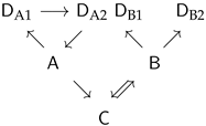
The following (arbitrarily constructed) example illustrates a combination of the special cases introduced above.
Information 10 00272 i005
Each individual link in this directed graph is a direct cause. C is multiply caused by A and B. A is a common (two-fold) cause of C and D A 1 . B is a common (three-fold) cause of C, D B 1 , and D B 2 . D A 2 is an indirect cause of C mediated by A. C is an indirect cause of D B 1 and D B 2 mediated by B. The closed-loop triangle formed by the subgraph A, D A 1 , and D A 2 illustrates circular causation, which can also be considered as a loop of three direct or indirect cause-effect relations. The relation between B and C is bidirectional, an even simpler case of circular causation. The nodes D B 1 and D B 2 have no causal effect at all on the remaining graph. They are causally inefficacious, a feature that is often called epiphenomenal in the philosophical discussion of mental states.
So far, all links have been treated as yes–no connections, whose entries in the adjacency matrix of a graph are either 0 or 1. (Interested readers may want to express the graph just discussed in terms of its adjacency matrix A M and take a look at its spectrum.) This restriction can be relaxed by permitting statistical or probabilistic causation, where links can be weighted by probabilities in the range between 0 and 1. For instance, varying the link between A and C in the illustration above allows us to control the influence of the triangle in the upper left on the rest of the graph. Moreover, it can be useful to consider so-called signed graphs with positive and negative links for particular applications such as social networks [30].
Even more radical examples of statistical causation exist in quantum mechanics. For instance, an ensemble of (radioactively) decaying atoms follows the law of exponential decay statistically. This law predicts the probability for individual atoms to decay as a function of time, but tells us nothing about the actual decay time of each single atom. This is a generic feature in many aspects of quantum theory, where chance events are ontic rather than epistemic (i.e., due to lacking knowledge or ignorance, as in statistical physics).

3. Synchronic Correlations

This section asks how to understand correlations that are synchronic rather than diachronic. Synchronic correlations do not extend over time, and hence involve no predictive or causal aspects in the sense of gathering knowledge about the future from past and present. In this spirit, they could be called (in a temporal sense) “nonlocal”—a term that we will reserve for quantum correlations though, for which it has received most attention.
If correlations do not involve temporal dependencies, they typically express regularities in datasets without temporal order. This is relevant for most of big data science and methods of data mining to identify clusters of data giving rise to patterns (Section 3.1). It is particularly relevant for multiscale systems whose behavior can be studied at various levels of resolution, defining different domains of discourse. A pertinent example is how various scales of granularity in brain activity, from neurons to overall brain electric potentials, are correlated with one another (Section 3.2).
More generally, Nagel [31] suggested the fitting notion of “bridge laws” for laws connecting domains of discourse. They are important in the discussion of interlevel relations such as reduction, supervenience and emergence. In areas such as cognitive neuroscience or consciousness studies these concepts aquired a lot of attention recently in the context of so-called “neural correlates of consciousness” or the mental–physical relationship in general (Section 3.4). Since some novel developments in this direction are inspired by quantum theoretical ideas, the acausal nature of quantum correlations will also be addressed along the way (Section 3.3).

3.1. Data Mining

The goal of data mining is the discovery of new, previously unknown knowledge from relations among data that can be unveiled in large data bases [32,33]. The way to do so is the exploratory detection of patterns, correlations or statistical dependencies that serve to cluster data. There is some common ground of data mining with the field of machine learning, with the goal to have machines learn from data. While machine learning employs all kinds of learning—supervised, unsupervised, and by reinforcement—data mining typically works with unsupervised learning.
However, unsupervised clustering in data mining can be augmented by supervised learning techniques if training data are available in addition to the large data base to be classified by clustering. For instance, if huge numbers of undiagnosed images are to be classified in medical studies, this may be facilitated if a small number of diagnosed data are available for training purposes. Corresponding hybrid techniques are called semisupervised.
A hallmark of data mining is that the data are collected without preconceived hypotheses. This is at variance with the classic research strategy that a hypothesis about some phenomena is first posited and then tested by data specifically collected for that purpose. Therefore, data mining is an exploratory practice, it is not oriented toward anything like a proof of evidence. This raises the issue of how valid the results of such exploratory studies are, and how their validity can be assessed.
If a pattern detection algorithm (or clustering algorithm) assigns data to patterns (clusters of data points), this leads to a classification. Often, the correlations between data points in an obtained cluster can be statistically significant and yet spurious. As Ramsey theory predicts ([10]; see Section 1), the number of spurious correlations explodes as data bases become larger. So validity checks are of utmost importance to separate meaningful from spurious clusters.
The pertinent literature [34] offers a taxonomy of validity (quality) checks by criteria using multivariate correlations between data due to proximity or similarity measures or cohesion, separation, and silhouette coefficients in networks or graphs. Many validity assessments operate with the stability or robustness of a classification with respect to perturbations [35]. Roughly, the validity of a cluster is high if its robustness against perturbations is high. Similarly, if a given clustering is a good predictor for clusters from different datasets, its validity is considered high [36]. However, note that a predictor in this sense is a classifier, it is not about predicting the future from the past (as in Section 2.1).
Another problem with data mining is that the number of patterns to be found is usually not prescribed and has to result from the clustering procedure. A worst case scenario in this respect is that an increasing number of clusters does not essentially change the clustering quality; this becomes even harder if fuzzy rather than crisp clusters have to be admitted due to the data structure. Additional problems arise for data from complex multiscale systems, e.g., biological or cognitive systems, where clusters are to be expected at different scales that may be a priori unknown (hierarchical clustering). Needless to say, clustering in complex systems becomes even more difficult if no scales can be separated.

3.2. Correlations Across Domains

Relationships between different domains of scientific descriptions of particular phenomena are expressed by atemporal, synchronic correlations. Although domains generally cannot be assumed to be ordered hierarchically, one often speaks of lower and higher levels of description, where lower levels are (in some sense) considered as more fundamental. Systems with multiple levels of description are also known as multilevel systems. As a rule, the behavioral levels of a multilevel system can be distinguished—and often defined—by different scales in space and time. Hence they are also called multiscale systems.
From a systematic point of view, there are four possibilities to relate higher- and lower-level properties.
(1) The description of properties in a particular lower-level domain of description (including its laws) offers both necessary and sufficient conditions to derive the description of properties in a higher-level domain. This is a strict form of reduction. It was most popular under the influence of positivist thinking in the mid-20th century, but does in fact not work for many examples one initially thought it would work for [31]. Reductive explanations in this sense would be candidates for one-to-one correlations between domains
(2) The description of properties in a particular lower-level domain of description (including its laws) offers neither necessary nor sufficient conditions to derive the description of properties in a higher-level domain. This represents a form of radical emergence insofar as there are no relevant conditions connecting the domains. This picture of a patchwork of unconnected domains (Cartwright [37]) appears somewhat pointless if one is actually interested in such connections.
(3) The description of properties in a particular lower-level domain of description (including its laws) offers sufficient but not necessary conditions to derive the description of properties in a higher-level domain. This version includes the idea that a lower-level description offers multiple realizations of a particular property at a higher level—a feature characteristic of supervenience (Kim [38]). Multiple realization (not to be confused with diachronic multiple causation) implies many-to-one correlations between lower and higher levels.
(4) The description of properties in a particular higher-level domain of description (including its laws) offers necessary but not sufficient conditions to derive the description of properties in a lower-level domain. This version, for which Bishop and Atmanspacher [39] proposed the notion of contextual emergence, indicates that higher-level contingent contextual conditions are required in addition to the lower-level description for the derivation of higher-level properties. Without the specification and implementation of such higher-level contexts, correlations between lower and higher levels would be one-to-many.
Typically, the granularity of microstates at a lower level in a multiscale system is finer than that of macrostates at a higher level. This leads to the problem to find a proper partition (clustering in the terminology of Section 3.1) of microstates that yields meaningful higher-level macrostates. A much discussed example for correlations between micro- and macrostates refers to the momentum and energy of individual particles in a many-particle system at the lower level of point mechanics and temperature and entropy at the higher level of thermodynamics. The relation between them is the well-known bridge law
E kin = 3 / 2 k T ,
relating the mean kinetic energy E k i n of the particles to temperature T via Boltzmann’s constant k. While this example has often been presented as a case for (1), this interpretation does not survive closer scrutiny.
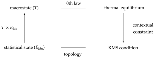
Today we know that the relation between thermodynamics and mechanics is more complicated, and resembles a “closed-loop” procedure (as indicated in Section 2.2) combining (3) and (4). Temperature relies on the context of thermal equilibrium through the zeroeth law of thermodynamics, which does not exist in statistical mechanics. However, thermal equilibrium states can be related to statistical mechanical states by a stability condition (the so-called KMS condition, due to Kubo, Martin, and Schwinger) implemented onto the mechanical state space [40,41]. The context of thermal equilibrium operates as a contextual constraint yielding the KMS state at the mechanical level. In this way, the relation between a thermal equilibrium state and the KMS state provides the sound foundation for the bridge law expressed above. (For a good overview and technical details see [42], Chapters 5–6, see also [13], Section 2.2, for an in-depth discussion accessible for the more general reader.)
The KMS condition induces a contextual topology, which determines a coarse-graining of the microstate space that serves the definition of statistical states (distributions). This partitioning of the state space into cells leads to statistical states that represent equivalence classes of individual microstates. They form ensembles of states that are indistinguishable with respect to their mean kinetic energy and can be assigned the same temperature. Differences between individual microstates falling into the same equivalence class are irrelevant with respect to emergent macrostates with a particular temperature. Note the interplay of top-down and bottom-up arrows that expresses a self-consistent (“circular” but not circularly causal) combination of supervenience (3) and contextual emergence (4).
Information 10 00272 i006
However, partitions as mentioned in the example above are not always straightforward to construct. In particular, complex nonlinear systems require cells of varying form and size rather than a uniform homogeneous partition. The mathematical theory of so-called generating partitions can be employed to find proper macrostates in such cases. The key criterion to do so is the stability of a generating partition under the microstate dynamics, so that the resulting macrostates are robustly defined and their dynamics is a faithful (topologically conjugate) representation of the microstate dynamics. In this procedure, level-specific temporal dynamics is exploited to reliably construct an atemporal relation between levels avoiding granularity mismatches [43] and securing meshing dynamics [44].
[Remark: Two mappings f : X X and g : Y Y on topological spaces X , Y are topologically conjugate if there exists an invertible intertwiner mapping π : Y X such that g = π 1 f π . In dynamical systems, the dynamics of microstates is topologically conjugate with a symbolic (macrostate) dynamics if the macrostates are based on a generating partition. Although generating partitions are exactly known only for a few cases, there are techniques to approximate them in general situations.] An important nuance in this picture is that it does not work without knowledge about the context of the higher level. This context yields a top-down constraint, or downward confinement for the lower level. As we saw above, the bridge law relating kinetic energy and temperature derives from implementing the higher-level context of thermal equilibrium at the lower, mechanical level. The terms “downward causation” or “top-down causation” [45] are infelicitous choices for addressing downward confinement by contextual constraints. More details and several applications are given in [46], see also [47].
There are several ways to express one-to-many mappings formally. A very fundamental one among them works with symmetries and their breakdown. Generally speaking, a symmetry is defined by the invariance of some property under transformations. Identifying an invariant property means to identify subsets of microstates whose differences are irrelevant with respect to this invariant property. In this sense, a partition into cells of microstates defining macrostates exploits symmetries at the microstate level. Symmetry arguments can be seen as formal causation and have turned out to be extremely powerful tools in the development of theoretical physics, but their range of applications is not exhausted by it.

3.3. Nonlocal Quantum Correlations

In the early days of quantum mechanics, Einstein et al. [48] published a thought experiment for which quantum mechanics predicts nonlocal correlations with which the authors tried to demonstrate how absurd quantum mechanics would be without a classical local background theory. Later, Bell [49] designed an ingenious argument based on which these correlations can be empirically tested by violations of an inequality that reflects the classical situation. Aspect et al. [50], and many others after them, performed the corresponding experiments and showed that the Bell inequalities are violated indeed. This violation rules out so-called local hidden variables, which Einstein et al. [48] had been looking for, underneath an indeterministic quantum reality. This needs to be explained a bit (we try to stay as simple as possible within a standard Copenhagen-style picture). The state of an entangled quantum system, for example the state (in Diac notation) | Φ pair of a particle pair, is not the same as the product of the states | Φ 1 and | Φ 2 of two separate particles. We write this as | Φ pair | Φ 1 | Φ 2 . The decomposed states of the two separate particles arise from the pair state as soon as a property of the system, like spin, is measured: | Φ pair | Φ 1 | Φ 2 . Together with a spin measurement at particle 1, the opposite spin becomes realized at particle 2, so that there are strict anticorrelations between the measured spins of the two separate particle states. Note that the decomposition into states | Φ 1 and | Φ 2 is not universally prescribed but depends on the measurement interaction, so measurement is in fact a creative act.
[Remark: A basic example of an entangled pair state is a singlet state for two spin-1/2 particles (specified by indices 1 and 2 with spin-up | or spin-down | : | Φ singlet = 1 2 ( | 1 | 2 | 1 | 2 ) . Evidently, the entangled state | Φ pair cannot be written as a product of single-particle spin states | Φ 1 and | Φ 2 . The singlet state is one of four possible Bell states exhibiting entanglement of 2 qubits. Well-known entangled 3-qubit states are Greenberger-Horne-Zeilinger (GHZ) states. In principle, entanglement can comprise arbitrarily many subsystems.]
Bell’s inequality expresses the classical assumption of a local reality where the entangled pair state would in fact be the same as the product state of the two separate particles. In the formulation by Clauser et al. [51], this inequality reads:
| E ( a , b ) E ( a , b ) + E ( a , b ) + E ( a , b ) | 2
Here a and a are measurement settings for particle 1, b and b are measurement settings for particle 2, and E ( . , . ) expresses the expectation value of the measured spin pairs (+1,+1), (+1, 1 ), ( 1 ,+1), and ( 1 , 1 ) at particles 1 and 2 (+1/ 1 stand for up/down). Calculating these values of E for measurements with different settings yields that their sum violates the limit posed by classical correlations, the value 2, exactly in the way quantum mechanics predicts, namely up to the value 2 2 .
After many such experiments there is today no reasonable doubt about nonlocal quantum correlations as a salient feature of entangled quantum systems. While quantum mechanics began as the project to finalize the atomistic picture of physical reality dominant at the late 19th century, it has turned into the oppposite, a holistic framework of thinking, by the late 20th century. An excellent account of this historic development is due to Gilder [52], and a detailed conceptual analysis is due to Maudlin [53]. [Remark: While early entanglement experiments were still contaminated by loopholes leaving space for classical local realist interpretations, such loopholes have been closed over the years. Crucial experiments in this respect were performed recently [54,55,56] for the so-called detection loophole. For spectacular experiments on the freedom-of-choice loophole see [57,58].]
As a brief interlude, it should be mentioned that the range in which Bell’s inequalities can be violated in principle exceeds the quantum limit 2 2 , the so-called Tsirelson bound, up to the value of 4. Abstract examples to this effect have been constructed, but it is unclear at present what nature wants to tell us with these super-quantum correlations. Their study has become a vivid field of contemporary research, as the review by Popescu [59] demonstrates.
With some experimental sophistication one can exclude that the correlations could be a consequence of direct causal signals between the two particles. This can be done by space-like separated measurements, which preclude that a signal transmitting the result from particle 1 can reach particle 2 before particle 2 is measured. Rather, the correlations are a consequence of the nonlocal, or holistic, nature of the pair state from which they arise. This situation seems to resemble the scheme of a classical common cause discussed in Section 2.2.
Information 10 00272 i007
However, this is not the case either. For a classical common cause the causal pathways from the pair state to the separate subsystem states would be fully determinate from the outset. Whatever a classical pair state may be, e.g., a pair of socks, there would always be a right sock and a left sock prespecified before measurement. But this is not what the quantum experiment reveals. Although the measured spins of | Φ 1 and | Φ 2 turn out to be strictly anti-correlated, the first spin measurement has a completely random, indeterminate result (50 % +1 and 50% 1 ) – which then strictly determines the second result by correlation. Therefore, the initial state | Φ pair is no sufficient efficient classical common cause for the decomposed states | Φ 1 and | Φ 2 with their strictly correlated properties (Aristotle’s formal causation as indicated in the discussion of symmetries and their breakdown in Section 4.2 may be an appropriate way of looking at this situation).
Alternative to the standard way [53] to picture quantum entanglement, Bohm’s interpretation (see [60]) provides a fully deterministic picture for quantum measurements based on nonlocal hidden variables (encoded in the so-called quantum potential). On this account there is no indeterminateness in quantum measurements. And since its hidden variables are nonlocal, they are not in contradiction with Bell violations. Bohm called his interpretation causal and ontological, in order to emphasize its conceptual difference from stochastic and epistemic interpretations of quantum theory.
Another subtle point is the distinction between genuine efficient causation and causal implication. Genuine efficient causation is the influence of a cause on an effect, as mainly addressed in Section 2.2 of this essay. Causal implication, on the other hand, can be understood on the basis of counterfactual reasoning: for given events A and B, if B were different, then A would be different. On the standard picture, there is no (classical) efficient causation between the particles involved in quantum entanglement. But the correlated measurement results at particle 1 and particle 2 are causally implicated: if spin up were not the case at particle 1, spin down would not be the case at particle 2. The enigmatic finding of nonlocal quantum correlations (which Einstein called “spooky”) marks a major distinction between classical and quantum physics. Different from the classical sock example, we have to accept that an entangled quantum state does not have uniquely specified properties for the separate states emerging from measurement. In this sense, quantum measurements create properties and their values, which do not exist as such before the measurement is actually performed. Again, we are arguing within a Copenhagen-style picture, deliberately disregarding alternative accounts.
[Remark: The wikipedia entry at en.wikipedia.org/wiki/Interpretationsofquantummechanics lists 17+ different ways to interpret the formalism of quantum theory, each of which has different things to say about key conceptual aspects of entanglement. In this comparative essay we cannot possibly live up to their substance in detail and restrict ourselves to some common denominator, thereby paying the price of losing subtlety. See, e.g., [61] for more details.]
The unusual situation of correlations that can neither be interpreted as directly related causally nor due to a classical common cause keeps physicists and philosophers busy to look for numerous alternatives. The difference between states prior to and posterior to measurement calls for a metaphysical account distinguishing ontic and epistemic quantum realities [62,63] as different domains of discourse. For instance, Ismael and Schaffer [64] argue for a “common ground” principle that “casts nonseparable entities in a holistic light, as scattered reflections of a more unified underlying reality.” In another vein, Allen et al. [65] propose an option to generalize Reichenbach’s common cause principle to quantum causal models in a graph-theoretical framework.

3.4. Mind–Matter Correlations

This final section addresses a further kind of correlations for which there is no generally accepted way at present to interpret them properly: mind–matter correlations that relate the mental and the physical. It has to be acknowledged right away that the way to conceive of such correlations depends crucially on the adopted metaphysical framework. Yet the problems of understanding them does not mean that these correlations are not empirically established. In medical sciences, psychosomatic relationships are well known (e.g., the correlation between distress and heart rate), and neural correlates of consciousness are a key topic in thousands of publications in cognitive neuroscience.
As of today, there is no evidence for a cause-and-effect explanation in the sense of efficient causation for any of these mind–matter correlations. Nonetheless, plenitudes of imprudent statements such as “brain activity causes cognition” keep filling the literature, irrespective of how misleading, nonsensical, or not even wrong they are (see, e.g., [24] for pertinent examples and details). The truism that correlation is not causation is particularly relevant in behavioral and cognitive neuroscience.
How about the conceptual status of mind–matter correlations or, in other words, how about their metaphysical underpinnings? Reductive physicalists, arguably the mainstream in the study of mind and matter today, will see correlations between them as a pseudoproblem because for them the mental is either an illusion anyway or it has no causal power at all (compare point 1 in Section 3.2). Radical emergentists will not be concerned with them in the first place because they do not see any systematic regularities between the mental and the physical (compare point 2 in Section 3.2).
Cartesian-style dualism considers the mental and the physical as the two mutually exclusive substances of the world. Their correlations are thought of due to direct causal interactions between the two. On the other hand, the doctrine of the causal closure of the physical states that each physical phenomenon that has a cause has a physical cause. This raises the problem of how mental phenomena can be causally efficacious on physical states. This and related problems have been formulated in the famous trilemma of mental causation due to Bieri [66]. A nuanced discussion of understanding mental events as counterfactual causes (not efficient causes) is due to Harbecke [67]. However, a fourth metaphysical position, called dual-aspect monism offers a surprisingly elegant and parsimonious (but also challenging) way to make sense of mind–matter correlations. Sloppily speaking, dual-aspect monists regard the mental and the physical as epistemic aspects of an ontic base reality that itself is neither mental nor physical, but “psychophysically neutral”. So dual-aspect monism combines a base ontology with its derivative epistemologies. Using (and perhaps overstretching) Ismael and Schaffer’s [64] wording, the mental and the physical are “scattered reflections of a more unified underlying reality”.
For an overview of various recent dual-aspect accounts see [68]. One of them is due to a conjecture by Wolfgang Pauli and Carl Gustav Jung in the 1950s that has been developed and refined within recent decades (see [69]. We focus on this version (and disregard others) because it offers a truly innovative interpretation of mind–matter correlations that is not found elsewhere. In the Pauli-Jung conjcecture, the base reality is conceived holistically, so the distinction of mind and matter amounts to a decomposition of the underlying whole. Many other decompositions would be possible, and each one of them can be a basis for further ones. And, of course, compositions of decomposed domains are conceivable as well. Thus, this picture does not assume an “existence monism” in the sense that reality as such truly exists only as a whole. However, insofar as decomposition is prior to any subsequent compositional moves, the Pauli-Jung conjecture represents a “priority monism” in the sense of Schaffer [70].
The reason why Pauli, one of the main architects of quantum theory, saw dual-aspect monism as so vehemently fruitful for the mind–matter problem was that he realized a structural analogy between dual-aspect thinking and the quantum correlations introduced by entanglement in the study of the physical world. As Jung approached the undivided base of the psychophysically neutral through unconscious archetypal activity, Pauli approached it via quantum holism. And mind–matter correlations appear structurally analogous to the quantum correlations that are due to the decomposition of an entangled quantum state.
Information 10 00272 i008
The analogy is stunning indeed: just replace | Φ pair by the psychophysically neutral and | Φ 1 and | Φ 2 by the mental and the physical, and you get the same basic picture. Neither in physical entanglement nor in dual-aspect thinking are the correlations set up by causal interactions. However: while acausal quantum correlations between two particles | Φ 1 and | Φ 2 are purely statistical, correlations between the mental and the physical acquire a subjective element: they are experienced as meaningful. The meaning that constitutes the correlations is attributed by the experiencing subject. But that does not entail that this subjective attribution is arbitrary: it is an (often symbolic) expression of the non-subjective, psychophysically neutral, archetypal activity from which it originates.
The subjective experience of meaning is clearly something that physics or any other science with the pretense to describe and explain objective facts cannot address within its limits. (This observation resembles the difficulty—or impossibility?—to assess semantic information by purely syntactic correlation measures, as briefly touched in Section 1). It was Jung’s brillant and radical idea to propose experienced meaning itself as the constitutive element for a wide class of acausal and non-random correlations between the physical and the mental that he denoted as synchronistic events [71]. As a relational concept meaning connects subjective mental representations with what they represent in the physical domain.
[Remark: Two (or more) seemingly accidental, but not necessarily simultaneous events are called synchronistic if the following three criteria are satisfied. (1) Each pair of synchronistic events includes an internally conceived and an externally perceived component. (2) Any presumption of a direct causal relationship between the events is absurd or even inconceivable. (3) The events correspond with one another by a common meaning, often expressed symbolically. The first criterion expresses that synchronistic phenomena are psychophysical phenomena, intractable when dealing with mind or matter alone. The second criterion repeats the inapplicability of efficient causation in the narrow sense of a conventional cause-and-effect-relation. And the third criterion suggests the concept of meaning as a constructive way to characterize mind–matter correlations.]
The Pauli-Jung conjecture and its ramifications provide a most natural and straightforward interpretation of mind–matter correlations. Decomposing a holistic state into parts means to break its symmetry (again an example for formal causation) so that the emerging parts are connected by synchronic, atemporal correlations. A dual-aspect framework implies such correlations in the first place; there is no need to look for post hoc rationalizations for them, and also no need to declare them as mysterious.
Psychosomatic and psychoneural correlations are examples of “ordinary” mind–matter correlations that are fairly robust and, hence, reproducible. But there are also spontaneously occurring correlations, less robust and less well reproducible, that have been coined “exceptional experiences”. The Pauli-Jung conjecture suggests a way to accommodate all these kinds of correlations in one overarching conceptual framework. It implies that reproducibility as a strict criterion for scientific research should be relaxed—in a controlled way, so that a spectrum arises from strictly deterministic events over statistical distributions to meaningfully connected singular events.
[Remark: Atmanspacher and Fach [72] proposed to distinguish coincidence phenomena and dissociation phenomena for such extraordinary correlations. Systematically speaking, coincidence phenomena exhibit excess correlations beyond ordinary baseline correlations and include meaningful coincidences (synchronicities in Jung’s parlance). Conversely, dissociation phenomena exhibit deficit correlations where ordinary baseline correlations are disconnected, e.g., in out-of-body experiences, sleep paralysis etc. Note that this distinction is qualitative, based on the phenomenal experience of the correlations.]
It should be emphasized that an analogy, even if compelling, cannot be more than a starting point for more detailed work, both theoretically and empirically, that may support or disconfirm the analogy. In recent years, supporting evidence for the Pauli-Jung conjecture has been collected from data bases documenting exceptional experiences of thousands of individual subjects so far. The interested reader may find corresponding material in pertinent literature such as [72,73,74]. But we are still in the early phases of refining the conceptual framework toward a theory and testing its implications, and much more work waits to be done.

4. Some Conclusions

Correlations between observed data are at the heart of all empirical research that ultimately strives for establishing lawful regularities. But the laws, models and theories explaining these correlations have to be set up over and above the data themselves. In this general sense, correlations do not include their interpretation, and it is often a difficult task to substantiate interpretations that are meaningful.
This essay surveys various responses to this task in different areas, from well-established sciences to speculative contemporary areas of research. Its format as an overview entails that the complexities and profundities of various issues are not fully accounted for, and a number of details certainly remain uncovered. In such cases, references for further inquiry have been given to orient the inquisitive reader.
Diachronic correlations are correlations extending over time. Models to account for them are predictive or causal, while the pure correlations themselves are neither of the two. Both prediction and causation require a well-defined arrow of time to make sense. Examples such as proxy-data predictions, Granger “causality” and predictive processing belong to the realm of predictive models. Causal models include scenarios with single causes, multiple causes, common casuses, and so-called circular causes. Network or graph representations are suitable tools, not only to visualize all these kinds of causes and combinations thereof, but also to analyze and understand them.
Synchronic correlations are correlations for which no temporal order is known or which relate data from different domains of discourse. Due to the lack of temporal order, synchronic correlations cannot be interpreted in terms of temporal predictions or causal sequences. Data mining is a modern field of research in which clustering techniques together with validity criteria for the clusters obtained are used to distinguish meaningful correlations in data bases from spurious ones. Correlations between different descriptive domains, such as in complex multiscale or multilevel systems, are typical subjects of interdomain relations such as reduction, supervenience, and emergence.
A more sophisticated type of synchronic correlations are nonlocal quantum correlations. They have their common ground in a holistic (entangled) reality and differ fundamentally from classical common-cause schemes. Such quantum correlations, bizarre as they may seem on first glance, are now well understood and even used for technical applications. The most advanced, and speculative, kind of correlations addressed in this essay are correlations between the mental and the physical. Insofar as they exceed the domain of the physical as such, their nature cannot be sufficiently interpreted by physical regularities alone. Rather an extended framework of thinking is needed that includes both the mental and the physical, plus the largely unexplored relationship between them.
As mentioned before, this essay mainly focuses on the problem of how appropriate interpretations can be identified for observed correlations. In scientific methodology this is called inductive inference, and it is mainly data-driven. Its deductive counterpart, theory-driven approaches such as those based on symmetries whose breakdown is needed to predict observable phenomena remains largely unaddressed in this essay. Much work along these lines can be found in the history of physics. A most prominent example is Einstein’s discovery of special relativity, where time dilation, space contraction and the equivalence of mass and energy follow from the Lorentz-invariant formulation of classical mechanics. Pierre Curie [75] expressed the importance of symmetry breakings for empirical predictions from theory with his famous quote: “It is the dissymmetry that creates the phenomena.”
However, we would argue that coherent and comprehensive theories are usually not found on the basis of data alone. In the words of Wolfgang Pauli ([76], p. 38, translation HA):
I hope that no one still maintains that theories are deduced by strict logical conclusions from laboratory-books, a view which was still quite fashionable in my student days. Theories are established through an understanding inspired by empirical material, an understanding which is best construed ... as an emerging correspondence of internal images and external objects and their behavior. The possibility of understanding demonstrates again the presence of typical dispositions regulating both inner and outer conditions of human beings.

Funding

This work was supported by Collegium Helveticum through the project “Semantic Analysis of multiscale Health Dynamics”, where the extraction of meaning from data bases is crucial, both diachronically and synchronically. Collegium Helveticum is a transdisciplinary research institute jointly operated by ETH Zurich, the University of Zurich, and the Zurich School of Arts.

Acknowledgments

An earlier version of this paper benefitted from numerous suggestions by two referees, many of which gave rise to detailed commentary highlighted as remarks throughout the text.

Conflicts of Interest

The authors declare no conflicts of interest.

References

  1. Hume, D. A Treatise of Human Nature; Norton, D.F., Norton, M.J., Eds.; Clarendon: Oxford, UK, 2007. [Google Scholar]
  2. Pearson, K. Notes on regression and inheritance in the case of two parents. Proc. R. Soc. Lond. 1895, 58, 240–242. [Google Scholar]
  3. Asuero, A.G.; Sayago, A.; Gonzalez, A.G. The correlation coefficient. An Overview. Crit. Rev. Anal. Chem. 2006, 36, 41–59. [Google Scholar] [CrossRef]
  4. Anscombe, F.J. Graphs in statistical analysis. Am. Stat. 1973, 27, 17–21. [Google Scholar]
  5. Kantz, H.; Schreiber, T. Nonlinear Timer Series Analysis; Cambridge University Press: Cambridge, UK, 2010. [Google Scholar]
  6. Lyons, L. Open statistical issues in particle physics. Ann. Appl. Stat. 2008, 2, 887–915. [Google Scholar] [CrossRef]
  7. Fisher, R.A. Statistical Methods for Research Workers; Oliver and Boyd: Edinburgh, UK, 1925; p. 43. [Google Scholar]
  8. Ramsey, F.P. On a problem of formal logic. Proc. Lond. Math. Soc. 1930, s2-30, 264–286. [Google Scholar] [CrossRef]
  9. Erdös, P.; Rényi, A.; Sós, V.T. On a problem of graph theory. Stud. Sci. Math. Hung. 1966, 1, 215–235. [Google Scholar]
  10. Calude, C.S.; Longo, G. The deluge of spurious correlations in big data. Found. Sci. 2017, 22, 595–612. [Google Scholar] [CrossRef]
  11. Vygen, T. Spurious Correlations. Available online: http://www.tylervigen.com/spurious-correlations (accessed on 22 August 2019).
  12. Shannon, C.E.; Weaver, W. The Mathematical Theory of Communication; University of Illinois Press: Champaign, IL, USA, 1949. [Google Scholar]
  13. Atmanspacher, H. On macrostates in complex multiscale systems. Entropy 2016, 18, 426. [Google Scholar]
  14. AMS. Statement of the American Meterological Society. 2015. Available online: www.ametsoc.org/ams/index.cfm/about-ams/ams-statements/statements-of-the-ams-in-force/weather-analysis-and-forecasting/ (accessed on 22 August 2019).
  15. Granger, C.W.J. Investigating causal relations by econometric models and cross-spectral methods. Econometrica 1969, 3, 424–438. [Google Scholar] [CrossRef]
  16. Reichenbach, H. The Direction of Time; University of California Press: Berkeley, CA, USA, 1956. [Google Scholar]
  17. Rao, R.P.N.; Ballard, D.H. Predictive coding in the visual cortex: A functional interpretation of some extra-classical receptive-field effects. Nat. Neurosci. 1999, 2, 79–87. [Google Scholar] [CrossRef]
  18. Friston, K. Learning and inference in the brain. Neural Netw. 2003, 16, 1325–1352. [Google Scholar] [CrossRef] [PubMed]
  19. Wiese, W.; Metzinger, T. Vanilla PP for philosophers: A primer on predictive processing. In Philosophy and Predictive Processing; Metzinger, T., Wiese, W., Eds.; MIND Group: Frankfurt, Germany, 2017. [Google Scholar]
  20. Hinton, G.E. Learning multiple layers of representation. Trends Cognit. Sci. 2007, 11, 428–434. [Google Scholar] [CrossRef] [PubMed]
  21. Wilson, R.J. Introduction to Graph Theory; Oliver & Boyd: Edinburgh, UK, 1972. [Google Scholar]
  22. Pearl, J. Causality; Cambridge University Press: Cambridge, UK, 2009. [Google Scholar]
  23. Woodward, J.; Causation and Manipulability. Stanford Encyclopedia of Philosophy. 2016. Available online: https://plato.stanford.edu/entries/causation-mani/#InteCoun (accessed on 22 August 2019).
  24. Gomez-Marin, A. Causal circuit explanations of behavior: Are necessity and sufficiency necessary and sufficient? In Decoding Neural Circuit Structure and Function; Çelik, A., Wernet, M.F., Eds.; Springer: Berlin, Germany, 2017; pp. 283–306. [Google Scholar]
  25. Aristotle. Physics; Hackett Publishing: Cambridge, UK, 2018; pp. b17–b20. [Google Scholar]
  26. Falcon, A.; Aristotle on Causality. Stanford Encyclopedia of Philosophy. 2019. Available online: https://plato.stanford.edu/entries/aristotle-causality/ (accessed on 22 August 2019).
  27. Hitchcock, C.; Causal Models. Stanford Encyclopedia of Philosophy. 2018. Available online: https://plato.stanford.edu/entries/causal-models/ (accessed on 22 August 2019).
  28. Atmanspacher, H.; Filk, T. Determinism, causation, prediction and the affine time group. J. Conscious. Stud. 2012, 19, 75–94. [Google Scholar]
  29. El Hady, A. (Ed.) Closed-Loop Neuroscience; Elsevier: Amsterdam, The Netherlands, 2016. [Google Scholar]
  30. Harary, F. On the notion of balance of a signed graph. Mich. Math. J. 1953, 2, 143–146. [Google Scholar] [CrossRef]
  31. Nagel, E. The Structure of Science; Harcourt, Brace & World: New York, NY, USA, 1961. [Google Scholar]
  32. Cios, K.J.; Pedrycz, W.; Swiniarski, R.W.; Kurgan, L.A. Data Mining. A Knowledge Discovery Approach; Springer: Berlin, Germany, 2010. [Google Scholar]
  33. Han, J.; Kamber, M.; Pei, J. Data Mining: Concepts and Techniques; Morgan Kaufmann: Waltham, MA, USA, 2011. [Google Scholar]
  34. Xu, R.; Wunsch, D.C. Clustering; Addison-Wesley: Reading, UK, 2009. [Google Scholar]
  35. Lange, T.; Roth, V.; Braun, M.L.; Buhmann, J.M. Stability-based validation of clustering solutions. Neural Comput. 2004, 16, 1299–1323. [Google Scholar] [CrossRef] [PubMed]
  36. Tibshirani, R.; Walther, G. Cluste validation by prediction strength. J. Comput. Gr. Stat. 2005, 14, 511–528. [Google Scholar] [CrossRef]
  37. Cartwright, N. The Dappled World; Cambridge University Press: Cambridge, UK, 1999. [Google Scholar]
  38. Kim, J. Supervenience as a philosophical concept. Metaphilosophy 1990, 21, 1–27. [Google Scholar] [CrossRef]
  39. Bishop, R.C.; Atmanspacher, H. Contextual emergence in the description of properties. Found. Phys. 2006, 36, 1753–1777. [Google Scholar] [CrossRef]
  40. Haag, R.; Kastler, D.; Trych-Pohlmeyer, E.B. Stability and equilibrium states. Commun. Math. Phys. 1974, 3, 173–193. [Google Scholar] [CrossRef]
  41. Kossakowski, A.; Frigerio, A.; Gorini, V.; Verri, M. Quantum detailed balance and the KMS condition. Commun. Math. Phys. 1977, 57, 97–110. [Google Scholar] [CrossRef]
  42. Sewell, G.L. Quantum Mechanics and Its Emergent Macrophysics; Princeton University Press: Princeton, NJ, USA, 2002. [Google Scholar]
  43. Poeppel, D. The maps problem and the mapping problem: Two challenges for a cognitive neuroscience of speech and language. Cognit. Neuropsychol. 2012, 29, 34–55. [Google Scholar] [CrossRef] [PubMed]
  44. Butterfield, J. Laws, causation and dynamics at different levels. Interface Focus 2012, 2, 101–114. [Google Scholar] [CrossRef] [PubMed]
  45. Ellis, G.F.R. On the nature of causation in complex systems. Trans. R. Soc. S. Afr. 2008, 63, 69–84. [Google Scholar] [CrossRef] [Green Version]
  46. Atmanspacher, H.; beim Graben, P. Contextual emergence. Scholarpedia 2009, 4, 7997. Available online: http://www.scholarpedia.org/article/Contextual_emergence (accessed on 22 August 2019). [CrossRef]
  47. Shalizi, C.R.; Moore, C. What is a macrostate? Subjective observations and objective dynamics. arXiv 2003, arXiv:cond-mat/0303625. [Google Scholar]
  48. Einstein, A.; Podolsky, B.; Rosen, N. Can quantum-mechanical description of physical reality be considered complete? Phys. Rev. 1935, 47, 777–780. [Google Scholar] [CrossRef]
  49. Bell, J.S. On the Einstein-Podolsky-Rosen paradox. Physics 1964, 1, 195–200. [Google Scholar] [CrossRef]
  50. Aspect, A.; Grangier, P.; Roger, G. Experimental realization of Einstein-Podolsky-Rosen-Bohm Gedankenexperiment: A new violation of Bell’s inequalities. Phys. Rev. Lett. 1982, 49, 91–94. [Google Scholar] [CrossRef]
  51. Clauser, J.F.; Horne, M.A.; Shimony, A.; Holt, R.A. Proposed experiment to test local hidden-variable theories. Phys. Rev. Lett. 1969, 23, 880–884. [Google Scholar] [CrossRef]
  52. Gilder, L. The Age of Entanglement; Vintage: New York, NY, USA, 2009. [Google Scholar]
  53. Maudlin, T. Non-Locality and Relativity; Wiley: New York, NY, USA, 2011. [Google Scholar]
  54. Giustina, M.; Versteegh, M.A.M.; Wengerowsky, S.; Handsteiner, J.; Hochrainer, A.; Phelan, K.; Steinlechner, F.; Kofler, J.; Larsson, J.-A.; Abellán, C.; et al. Significant-loophole-free test of Bell’s theorem with entangled photons. Phys. Rev. Lett. 2015, 115, 250401. [Google Scholar] [CrossRef]
  55. Hensen, B.; Bernien, H.; Dréau, A.E.; Reiserer, A.; Kalb, N.; Blok, M.S.; Ruitenberg, J.; Vermeulen, R.F.L.; Schouten, R.N.; Abellán, C.; et al. Experimental loophole-free violation of a Bell inequality using entangled electron spins separated by 1.3 km. Nature 2015, 526, 682–686. [Google Scholar] [CrossRef] [PubMed]
  56. Shalm, L.K.; Meyer-Scott, E.; Christensen, B.G.; Bierhorst, P.; Wayne, M.A.; Stevens, M.J.; Gerrits, T.; Glancy, S.; Hamel, D.R.; Allman, M.S.; et al. A strong loophole-free test of local realism. Phys. Rev. Lett. 2015, 115, 250402. [Google Scholar] [CrossRef] [PubMed]
  57. Li, M.-H.; Wu, C.; Zhang, Y.; Liu, W.-Z.; Bai, B.; Liu, Y.; Zhang, W.; Zhao, Q.; Li, H.; Wang, Z.; et al. Test of local realism into the past without detection and locality loopholes. Phys. Rev. Lett. 2018, 121, 080404. [Google Scholar] [CrossRef] [PubMed]
  58. Rauch, D.; Handsteiner, J.; Hochrainer, A.; Gallicchio, J.; Friedman, A.S.; Leung, C.; Liu, B.; Bulla, L.; Ecker, S.; Steinlechner, F.; et al. Cosmic Bell test using random measurement settings from high-redshift quasars. Phys. Rev. Lett. 2018, 121, 080403. [Google Scholar] [CrossRef] [PubMed]
  59. Popescu, S. Nonlocality beyond quantum mechanics. Nat. Phys. 2014, 10, 264–270. [Google Scholar] [CrossRef]
  60. Bohm, D.; Hiley, B.J. The Undivided Universe; Routledge: London, UK, 1993. [Google Scholar]
  61. Myrvold, W. Philosophical Issues in Quantum Theory. 2016. Available online: https://plato.stanford.edu/entries/qt-issues/#MeasProbForm (accessed on 22 August 2019).
  62. Atmanspacher, H.; Primas, H. Epistemic and ontic quantum realities. In Time, Quantum, and Information; Castell, L., Ischebeck, O., Eds.; Springer: Berlin, Germany, 2003; pp. 301–321. [Google Scholar]
  63. Harrigan, N.; Spekkens, R.W. Einstein, incompleteness, and the epistemic view of quantum states. Found. Phys. 2010, 4, 125–157. [Google Scholar] [CrossRef]
  64. Ismael, J.; Schaffer, J. Quantum holism: Nonseparability as common ground. Synthese 2016. [Google Scholar] [CrossRef]
  65. Allen, J.-M.A.; Barrett, J.; Horsman, D.C.; Lee, C.M.; Spekkens, R.W. Quantum common causes and quantum causal models. Phys. Rev. X 2017, 7, 031021. [Google Scholar] [CrossRef]
  66. Bieri, P. Analytische Philosophie des Geistes; Anton Hain Publisher: Königstein, Germany, 1981. [Google Scholar]
  67. Harbecke, J. Mental Causation; Walter de Gruyter: Berlin, Germany, 2008. [Google Scholar]
  68. Atmanspacher, H. 20th century variants of dual-aspect thinking (with commentaries and replies). Mind Matter 2014, 12, 245–288. [Google Scholar]
  69. Atmanspacher, H.; Fuchs, C.A. (Eds.) The Pauli-Jung Conjecture and Its Impact Today; Andrews UK Limited: Luton, UK, 2017. [Google Scholar]
  70. Schaffer, J. Monism: The priority of the whole. Philos. Rev. 2010, 119, 31–76. [Google Scholar] [CrossRef]
  71. Jung, C.G.; Pauli, W. The Interpretation of Nature and the Psyche; Pantheon: New York, NY, USA, 1955. [Google Scholar]
  72. Atmanspacher, H.; Fach, W. A structural-phenomenological typology of mind-matter correlations. J. Anal. Psychol. 2013, 58, 218–243. [Google Scholar] [CrossRef] [PubMed]
  73. Fach, W.; Atmanspacher, H.; Landolt, K.; Wyss, T.; Rössler, W. A comparative study of exceptional experiences of clients seeking advice and of subjects in an ordinary population. Front. Psychol. 2013, 4, 65. [Google Scholar] [CrossRef] [PubMed]
  74. Atmanspacher, H.; Fach, W. Exceptional experiences of stable and unstable mental states, understood from a dual-aspect point of view. Philosophies 2019, 4, 7. [Google Scholar] [CrossRef]
  75. Curie, P. Sur la symétrie dans les phénomènes physiques, symétrie d’un champ électrique et d’un champ magnétique. J. Phys. Theor. Appl. 1894, 3, 393–415. [Google Scholar] [CrossRef]
  76. Pauli, W. Phänomen und physikalische Realität. Dialectica 1957, 11, 36–48. [Google Scholar] [CrossRef]