MFA-OSELM Algorithm for WiFi-Based Indoor Positioning System

 ,
,
Abstract
:1. Introduction
2. Related Works
Review of Feature Adaptive Online Sequential Extreme Learning Machine (FA-OSELM)
- For every line, there is only one ‘1′; the rest of the values are all ‘0′;
- Every column has at most one ‘1′; the rest of the values are all ‘0′;
- signifies that following a change in the feature dimension, the ith dimension of the original feature vector will become the jth dimension of the new feature vector.
- Lower feature dimensions indicate that can be termed as an all-zero vector. Hence, no additional corresponding input weight is required by the newly added features;
- In cases where the feature dimension increases, if the new feature is embodied by the ith item of , a random generation of the ith item of should be carried out based on the distribution of .
3. Methodology
3.1. Generating Dynamic Scenarios of Localization
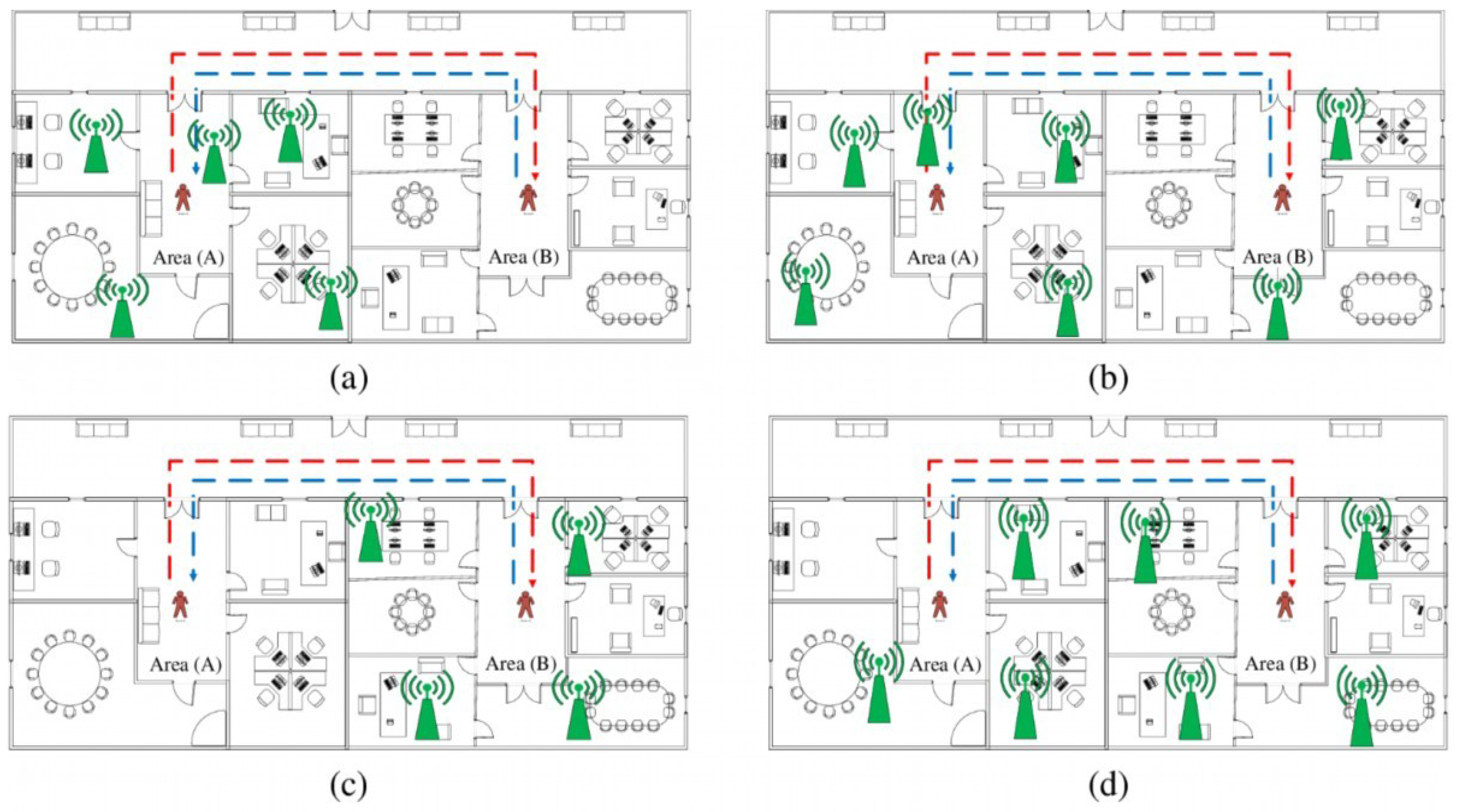
- The movement of a person from area A to area B. The number of APs in A () is higher than the number of APs in B (). The APs in B are contained in the APs in A, or . As shown in Figure 1a, the person then returns to area A. The red line signifies their trajectory from area A to area B, while the blue line denotes their trajectory from area B to area A. Based on the figure, it can be seen that all APs are contained in area A, which explains why .
- The person moves from area A to area B. is greater than or equal to . The APs in area B are not contained in the APs in area A, or . Then, the person returns to area A, as represented in Figure 1b. As in the previous scenario, the red line represents the trajectory from area A to area B, while the blue line represents the trajectory from area B to area A. It can be seen that the APs are distributed in both areas A and B, with greater AP density in area A, i.e., and .
- The person moves from area A to area B. is less than . The APs in area B are contained in the APs in area A, or . Then, the person returns to area A, as represented in Figure 1c. As in scenario 1, the APs are distributed in one area only; however, in this scenario, it is area B. Thus, .
- The person moves from area A to area B. is less than or equal to . The APs in area B are not contained in the APs in area A, or . Then, the person returns to area A, as represented in Figure 1d. As in scenario 2, the APs are distributed in both areas, however this time there is a higher AP density in area B.
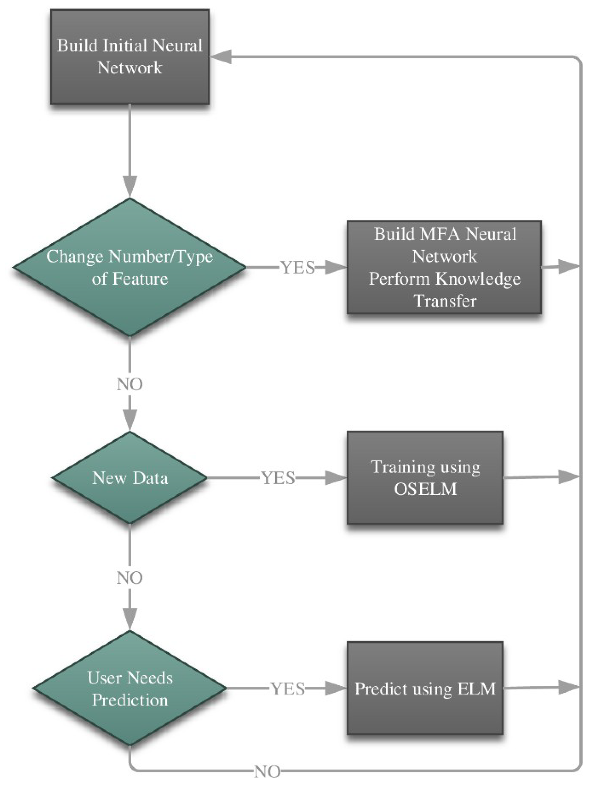
3.2. General Algorithmic Procedure
- Constructing the initial neural network;
- Constructing the maximum feature adaptive NN and carrying out transfer learning whenever a change in the number of features takes place;
- Impart training whenever data is accessible;
- Carry out prediction whenever a user request is required (or intermittently).
| Algorithm 1. Procedure of the maximum feature adaptive online sequential extreme learning machine (MFA-OSELM) for WiFi localization. |
|
3.3. Evaluation Measures
4. Experimental Results
4.1. Dataset Description and Pre-Processing
| Algorithm 2. Pseudocode for the dataset preparation for testing scenario 1. |
|
4.2. Results and Analysis
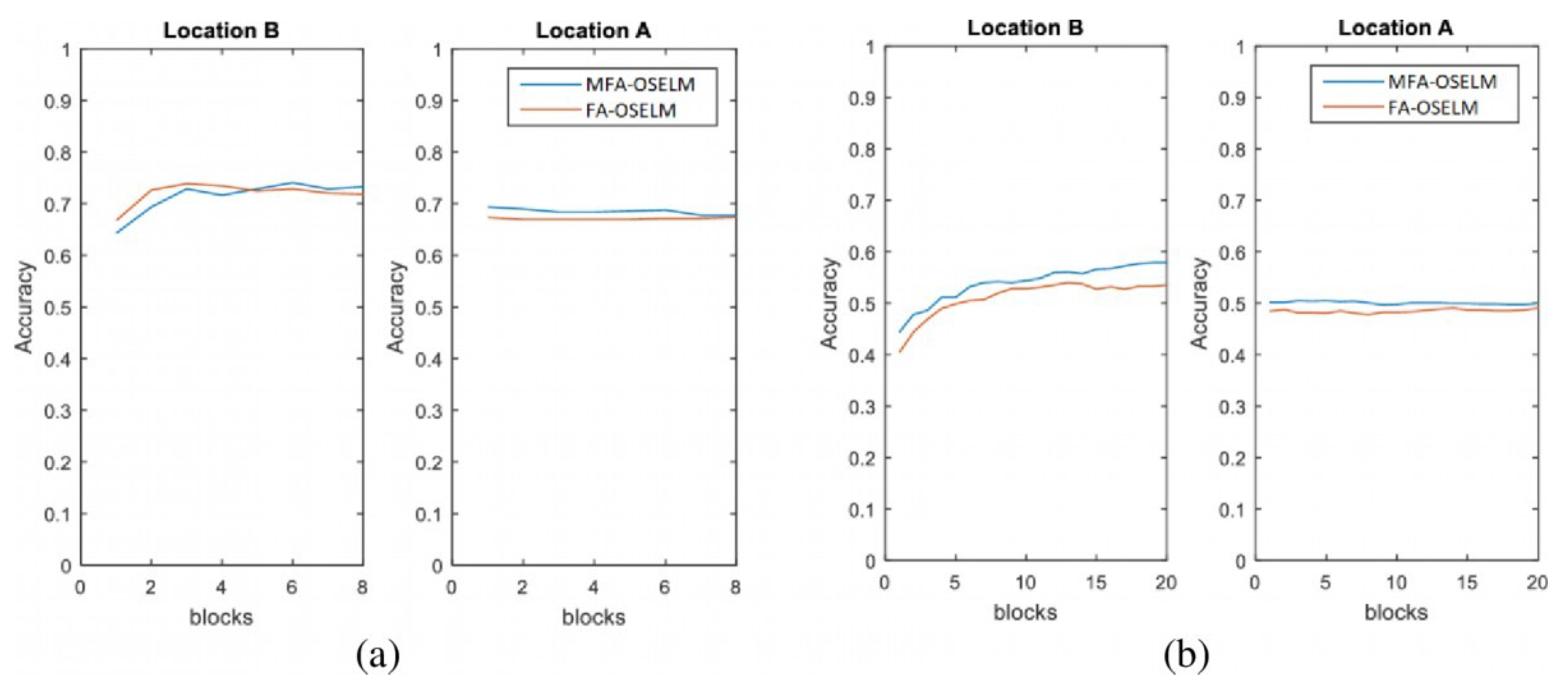
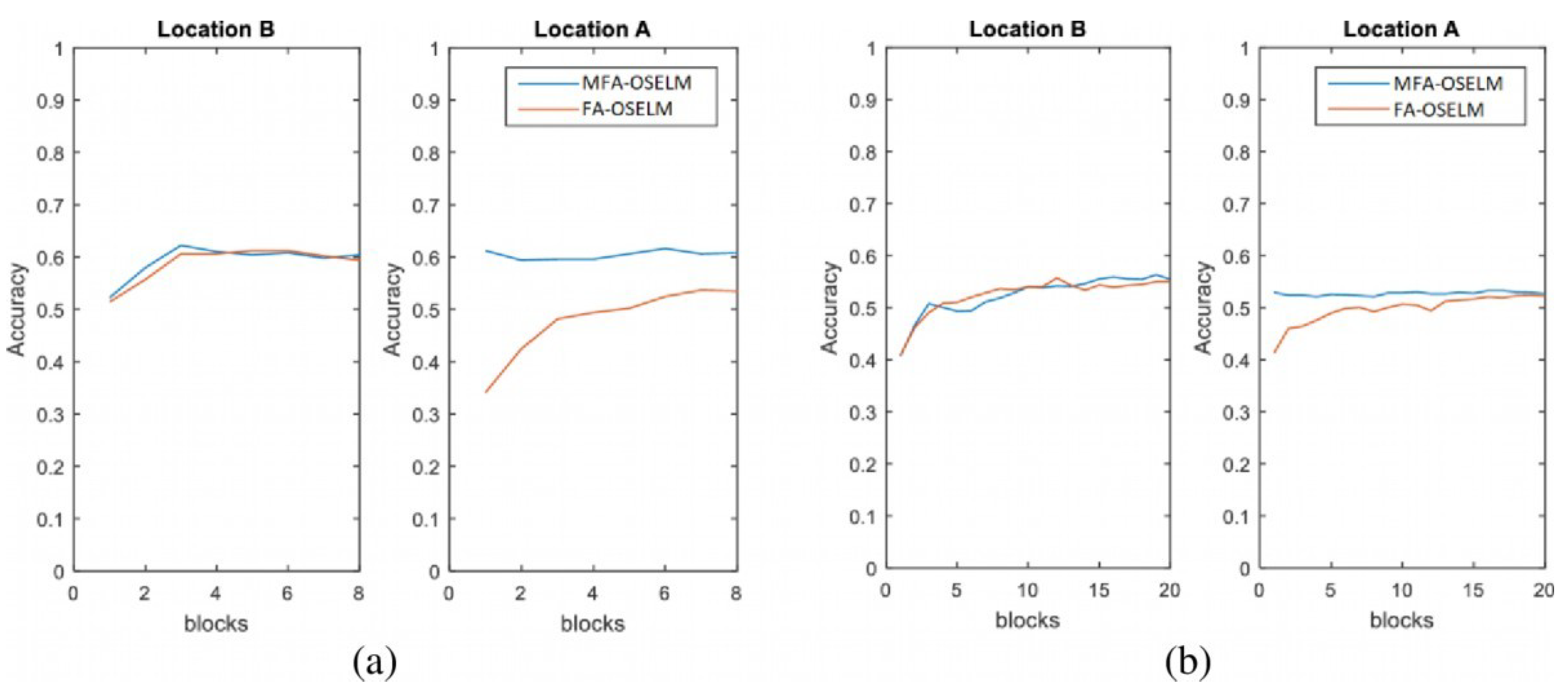
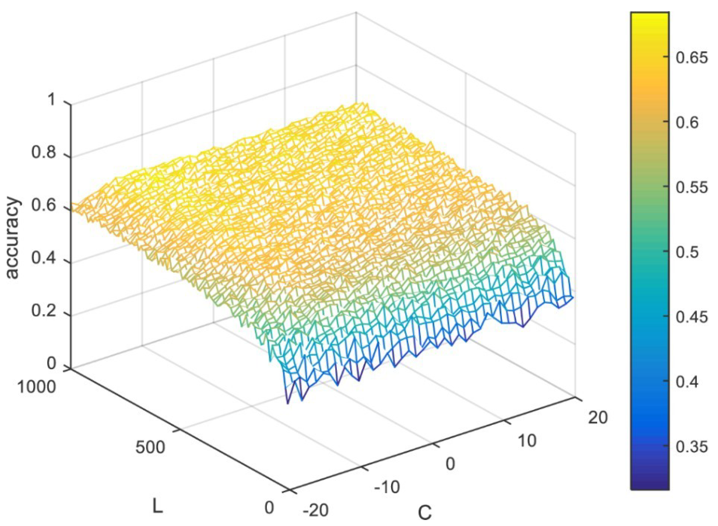
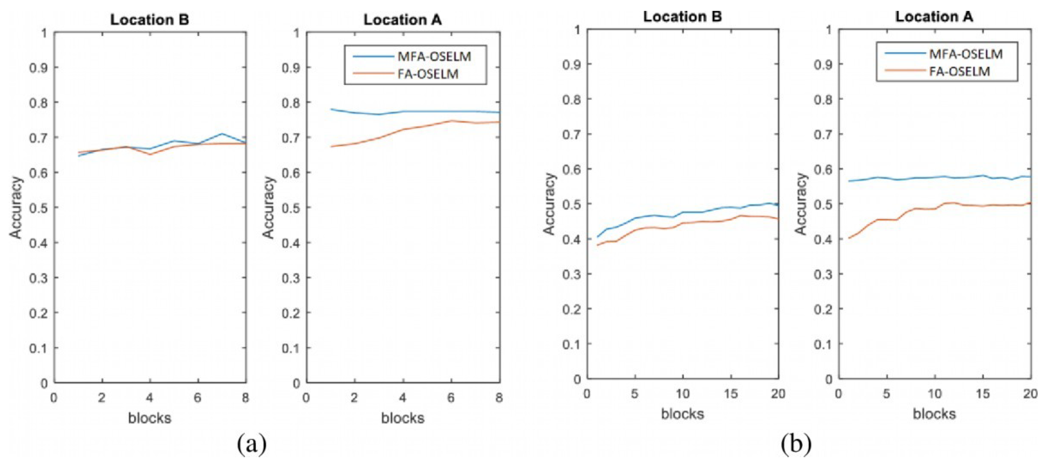
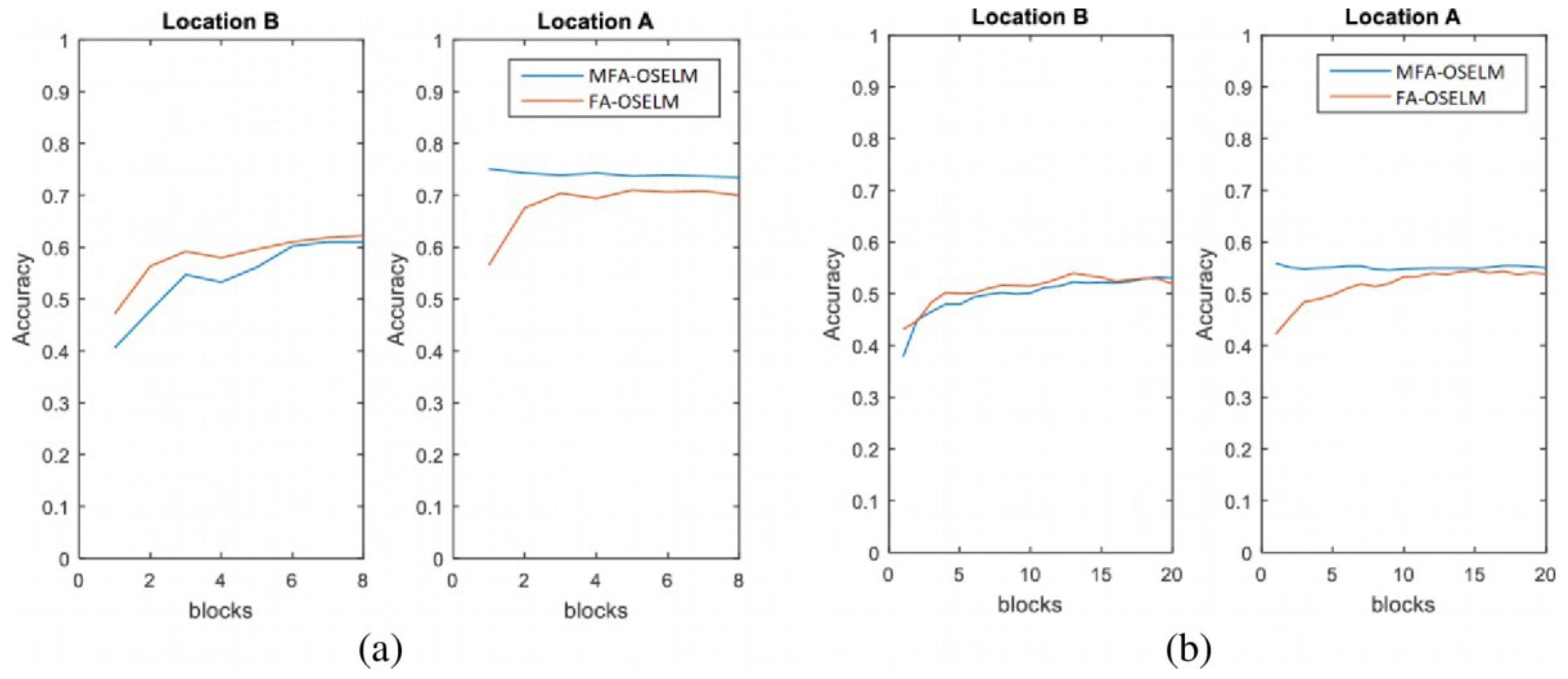
4.2.1. Accuracy
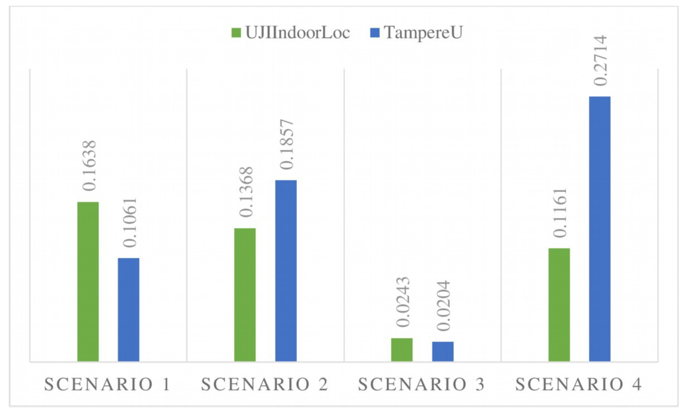
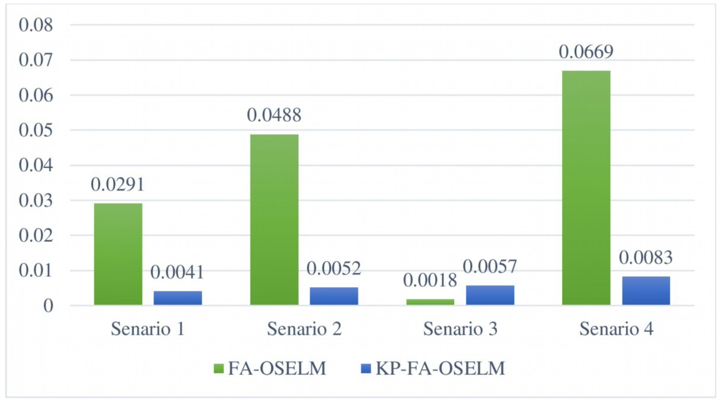
4.2.2. Maximum Accuracy Change
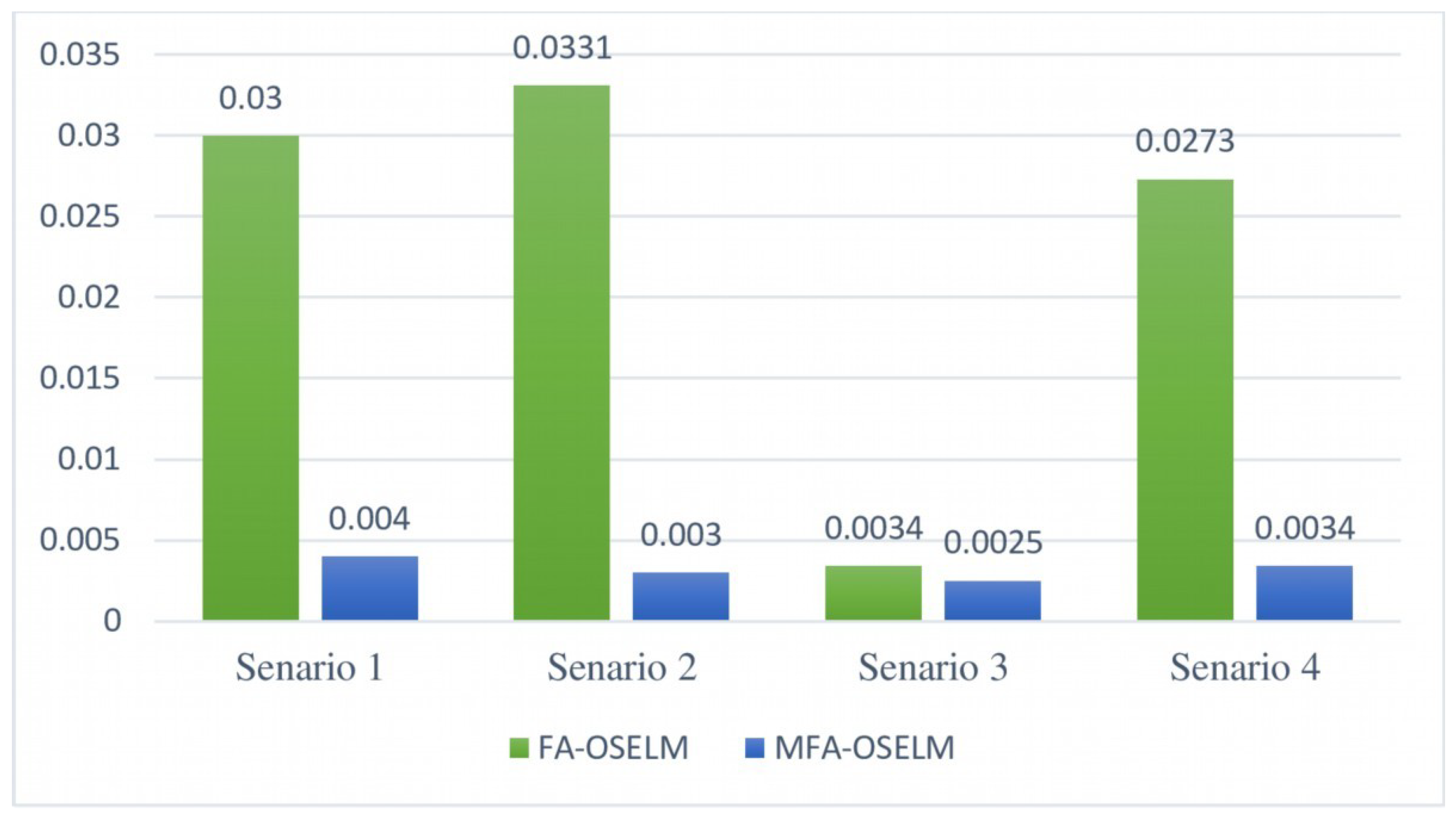
4.2.3. Standard Deviation
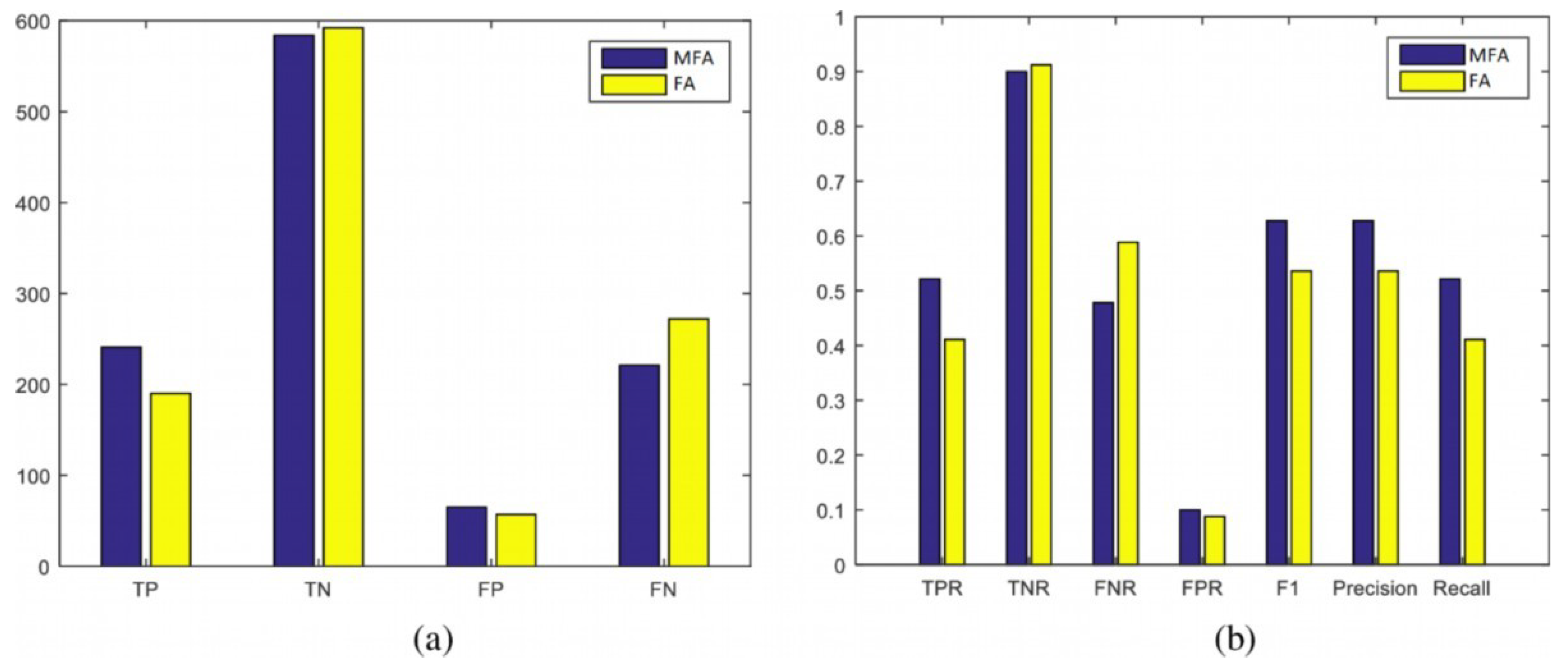
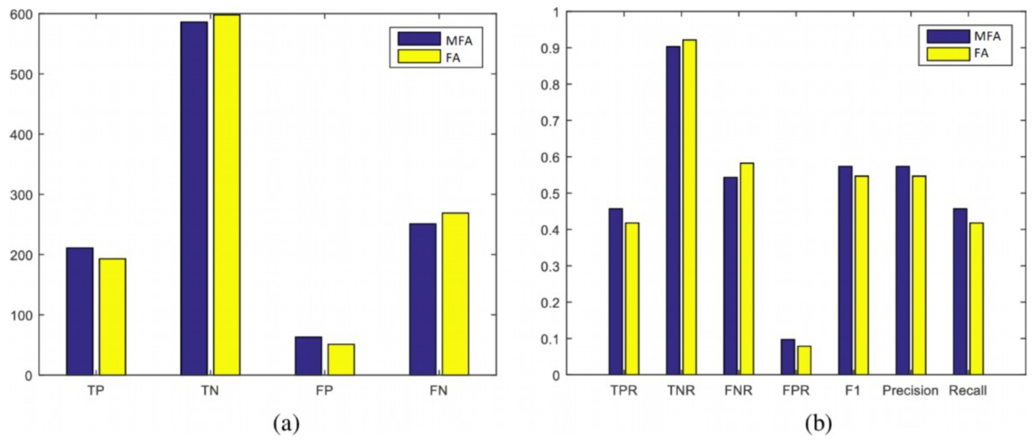
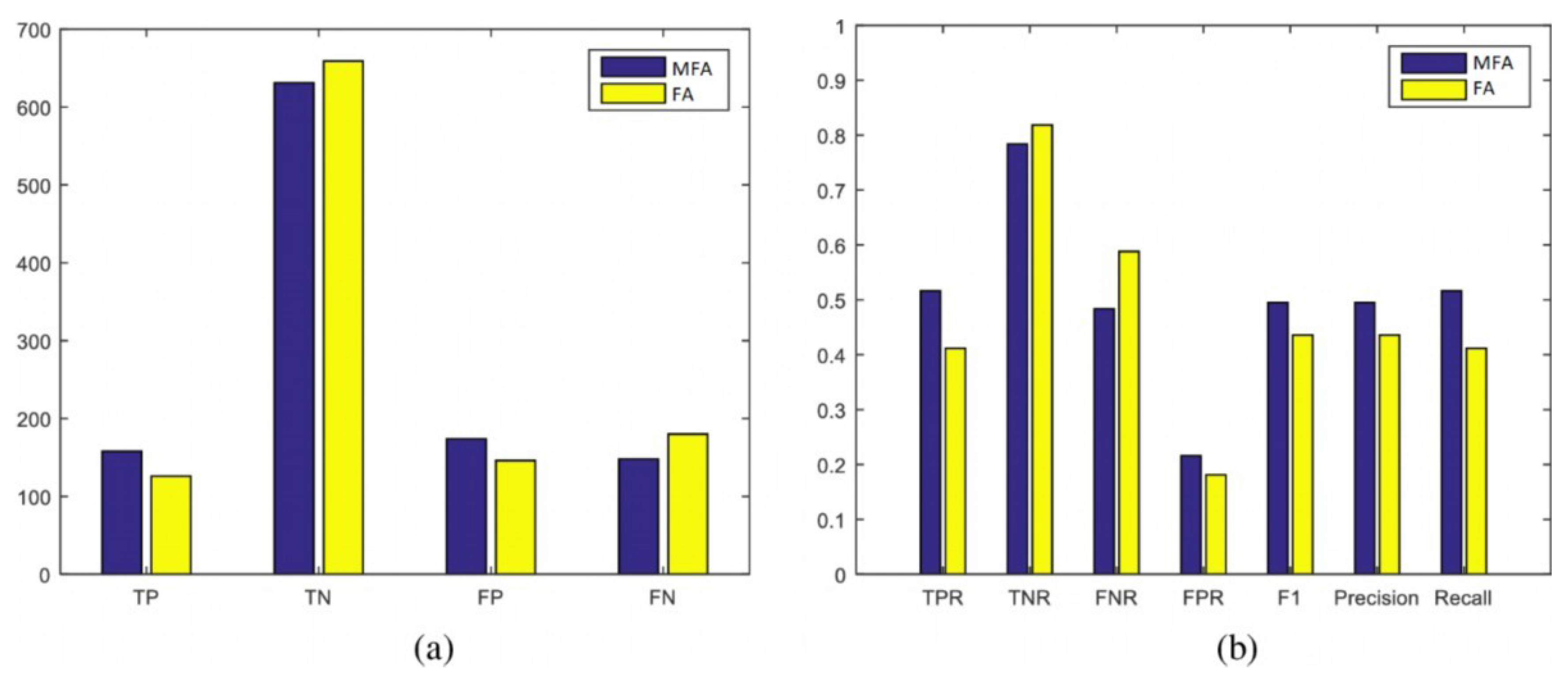
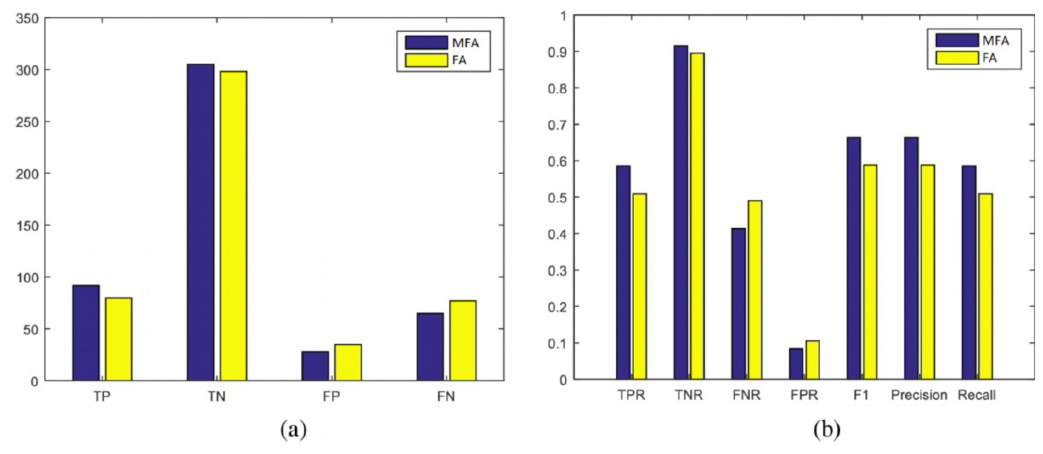
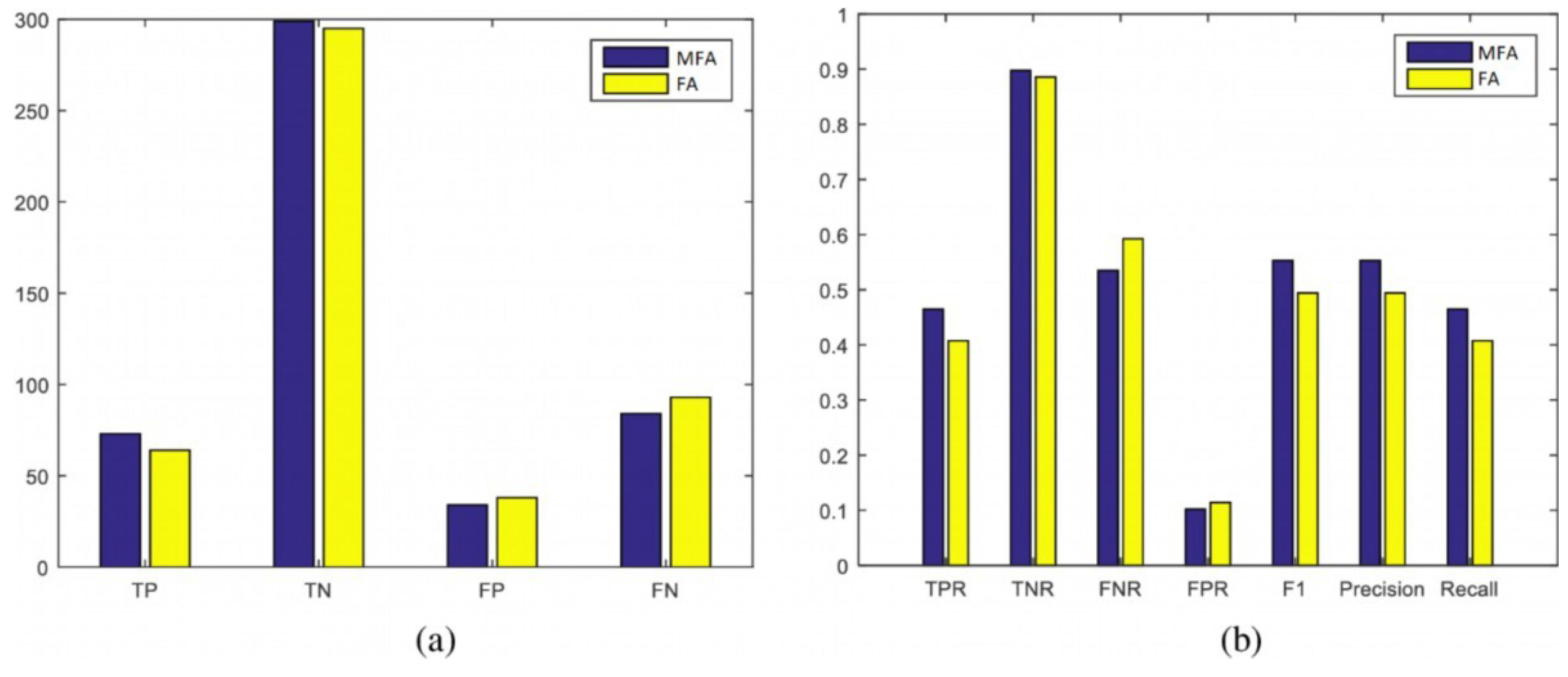
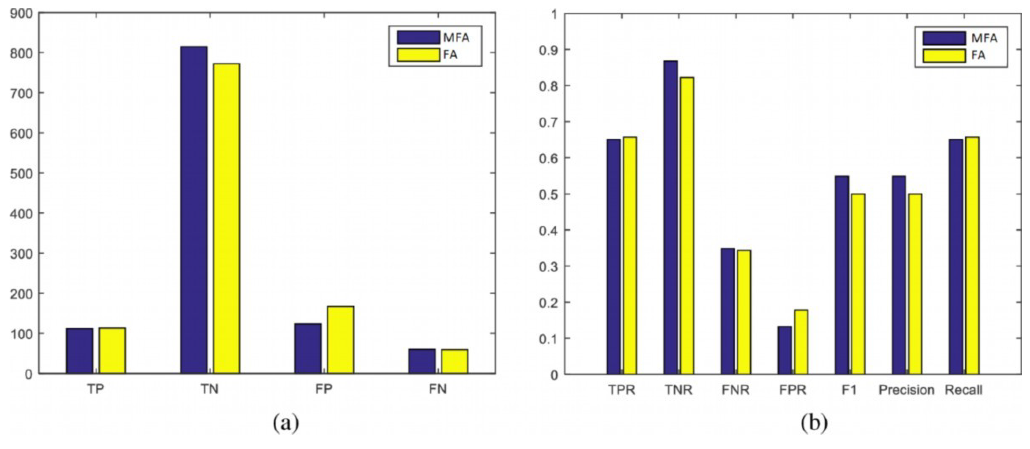
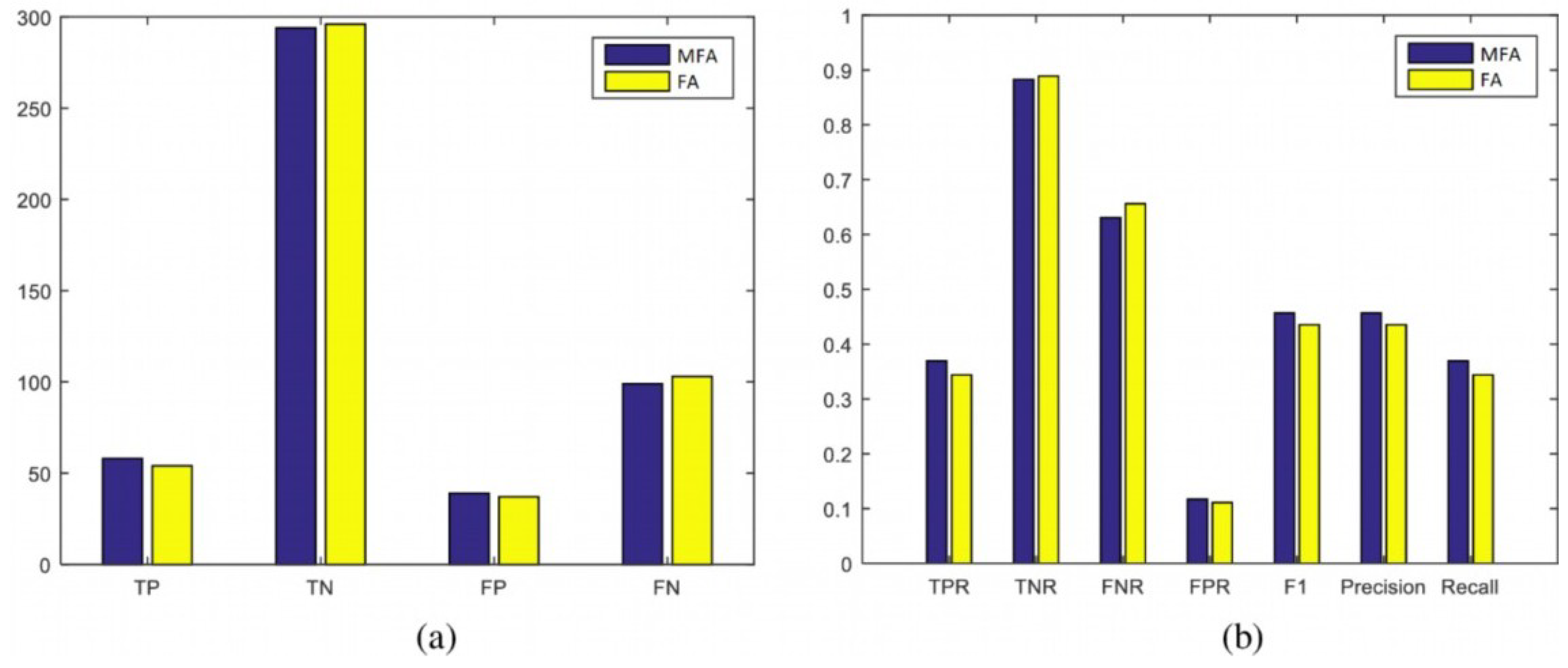
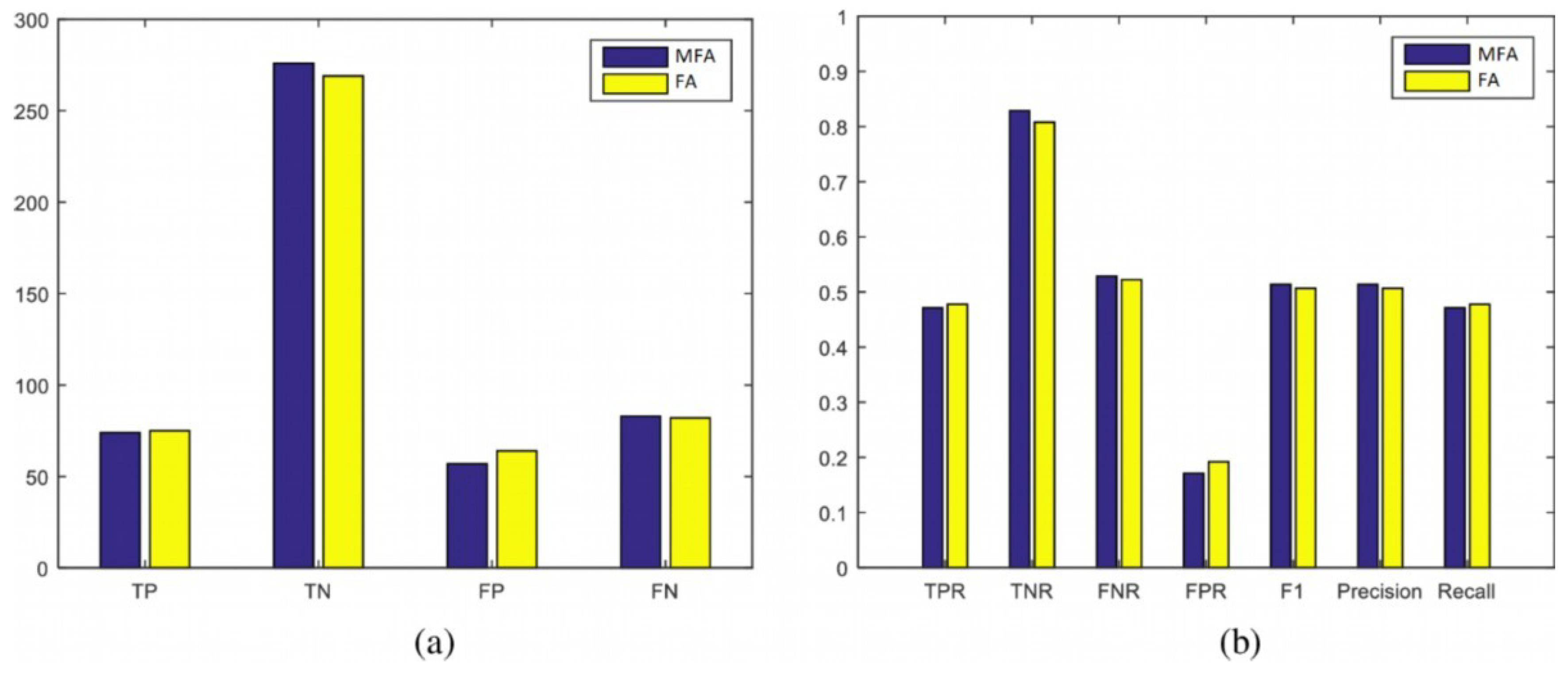
4.2.4. Classification Evaluation Measures
5. Summary and Future Work
Author Contributions
Funding
Conflicts of Interest
References
- Wan, J.; Zou, C.; Ullah, S.; Lai, C.F.; Zhou, M.; Wang, X. Cloud-enabled wireless body area networks for pervasive healthcare. IEEE Netw. Mag. 2013, 27, 56–61. [Google Scholar] [CrossRef]
- Xiao, J.; Zhou, Z.; Yi, Y. A Survey on Wireless Indoor Localization from the Device Perspective. ACM Comput. Surv. CSUR 2016, 49, 25. [Google Scholar] [CrossRef]
- Umanets, A.; Ferreira, A.; Leite, N. GuideMe—A Tourist Guide with a Recommender System and Social Interaction. Procedia Technol. 2014, 17, 407–414. [Google Scholar] [CrossRef]
- Wang, S.; Fidler, S.; Urtasun, R. Lost shopping! Monocular localization in large indoor spaces. In Proceedings of the IEEE International Conference on Computer Vision, Santiago, Chile, 7–13 December 2015; pp. 2695–2703. [Google Scholar] [CrossRef]
- Zou, H.; Zhou, Y.; Jiang, H.; Huang, B.; Xie, L.; Spanos, C. Adaptive localization in dynamic indoor environments by transfer kernel learning. In Proceedings of the Wireless Communications and Networking Conference (WCNC), San Francisco, CA, USA, 19–22 March 2017; pp. 1–6. [Google Scholar] [CrossRef]
- He, S.; Lin, W.; Chan, S.G. Indoor Localization and Automatic Fingerprint Update with Altered AP Signals. IEEE Trans. Mob. Comput. 2017, 16, 1897–1910. [Google Scholar] [CrossRef]
- Jiang, X.; Chen, Y.; Liu, J.; Gu, Y.; Chen, Z. Wi-Fi and Motion Sensors Based Indoor Localization Combining ELM and Particle Filter. In Proceedings of the ELM-2014; Cao, J., Mao, K., Cambria, E., Man, Z., Toh, K.A., Eds.; Springer: Cham, Switzerlands, 2015; Volume 2, pp. 105–113. [Google Scholar] [CrossRef]
- Pan, S.J.; Yang, Q. A Survey on Transfer Learning. IEEE Trans. Knowl. Data Eng. 2010, 22, 1345–1359. [Google Scholar] [CrossRef]
- Jiang, X.; Liu, J.; Chen, Y.; Liu, D.; Gu, Y.; Chen, Z. Feature Adaptive Online Sequential Extreme Learning Machine for lifelong indoor localization. Neural Comput. Appl. 2016, 27, 215–225. [Google Scholar] [CrossRef]
- Huang, G.; Zhu, Q.; Siew, C. Extreme learning machine: Theory and applications. Neurocomputing 2006, 70, 489–501. [Google Scholar] [CrossRef]
- Sun, Z.; Chen, Y.; Qi, J.; Liu, J. Adaptive Localization through Transfer Learning in Indoor Wi-Fi Environment. In Proceedings of the 2008 Seventh International Conference on Machine Learning and Applications Adaptive, San Diego, CA, USA, 11–13 December 2008; pp. 331–336. [Google Scholar] [CrossRef]
- Gu, Y.; Liu, J.; Chen, Y.; Jiang, X. Constraint Online Sequential Extreme Learning Machine for lifelong indoor localization system. In Proceedings of the International Joint Conference on Neural Networks, Beijing, China, 6–11 July 2014; pp. 732–738. [Google Scholar] [CrossRef]
- Mundo, L.B.D.; Ansay, R.L.D.; Festin, C.A.M.; Ocampo, R.M. A Comparison of Wireless Fidelity (Wi-Fi) Fingerprinting Techniques. In Proceedings of the 2011 International Conference on ICT Convergence (ICTC), Seoul, Korea, 28–30 September 2011; pp. 20–25. [Google Scholar] [CrossRef]
- Heidari, M.; Alsindi, N.A.; Pahlavan, K. UDP identification and error mitigation in ToA-based indoor localization systems using neural network architecture. IEEE Trans. Wirel. Commun. 2009, 8, 3597–3607. [Google Scholar] [CrossRef]
- Huang, G.; Zhu, Q.; Siew, C. Extreme Learning Machine: A New Learning Scheme of Feedforward Neural Networks. In Proceedings of the 2004 IEEE International Joint Conference on Neural Networks, Budapest, Hungary, 25–29 July 2004; Volume 2, pp. 985–990. [Google Scholar] [CrossRef]
- Huang, G.; Zhou, H.; Ding, X.; Zhang, R. Extreme Learning Machine for Regression and Multiclass Classification. IEEE Trans. Syst. Man Cybern. Part B Cybern. 2012, 42, 513–529. [Google Scholar] [CrossRef] [PubMed]
- Yim, J. Introducing a decision tree-based indoor positioning technique. Expert Syst. Appl. 2008, 34, 1296–1302. [Google Scholar] [CrossRef]
- Zheng, V.W.; Xiang, E.W.; Yang, Q.; Shen, D. Transferring localization models over time. In Proceedings of the Twenty-Third AAAI Conference on Artificial Intelligence, Chicago, IL, USA, 13–17 July 2008; pp. 1421–1426. [Google Scholar]
- Koweerawong, C.; Wipusitwarakun, K.; Kaemarungsi, K. Indoor localization improvement via adaptive RSS fingerprinting database. In Proceedings of the International Conference on Information Networking 2013, Bangkok, Thailand, 28–30 January 2013; Volume 1, pp. 412–416. [Google Scholar] [CrossRef]
- Lo, C.C.; Hsu, L.Y.; Tseng, Y.C. Adaptive radio maps for pattern-matching localization via inter-beacon co-calibration. Pervasive Mob. Comput. 2012, 8, 282–291. [Google Scholar] [CrossRef]
- Zou, H.; Jiang, H.; Lu, X.; Xie, L. An Online Sequential Extreme Learning Machine Approach to WiFi Based Indoor Positioning. IEEE World Forum Internet Things 2014, 2014, 111–116. [Google Scholar] [CrossRef]
- Lu, X.; Zou, H.; Zhou, H.; Xie, L.; Huang, G.B. Robust Extreme Learning Machine With its Application to Indoor Positioning. IEEE Trans. Cybern. 2016, 46, 194–205. [Google Scholar] [CrossRef] [PubMed]
- Zhang, M.; Wen, Y. Pedestrian Dead-Reckoning Indoor Localization Based on OS-ELM. IEEE Access 2018, 6, 6116–6129. [Google Scholar] [CrossRef]
- AL-Khaleefa, A.S.; Ahmad, M.R.; Isa, A.A.M.; Esa, M.R.M.; AL-Saffar, A.; Hassan, M.H. Feature Adaptive and Cyclic Dynamic Learning Based on Infinite Term Memory Extreme Learning Machine. Appl. Sci. 2019, 9, 895. [Google Scholar] [CrossRef]
- Al-Khaleefa, A.S.; Ahmad, M.R.; Isa, A.A.M.; Esa, M.R.M.; Al-Saffar, A.; Aljeroudi, Y. Infinite-Term Memory Classifier for Wi-Fi Localization Based on Dynamic Wi-Fi Simulator. IEEE Access 2018, 6, 54769–54785. [Google Scholar] [CrossRef]
- Zou, H.; Huang, B.; Lu, X.; Jiang, H.; Xie, L. A Robust Indoor Positioning System Based on the Procrustes Analysis and Weighted Extreme Learning Machine. IEEE Trans. Wirel. Commun. 2016, 15, 1252–1266. [Google Scholar] [CrossRef]
- Han, J.; Kamber, M.; Pei, J. 8—Classification: Basic Concepts. In Data Mining: Concepts and Techniques; Han, J., Kamber, M., Pei, J., Eds.; Elsevier: Boston, MA, USA, 2011; pp. 327–391. ISBN 978-0-12-381479-1. [Google Scholar]
- Torres-Sospedra, J.; Montoliu, R.; Martinez-Uso, A.; Avariento, J.P.; Arnau, T.J.; Benedito-Bordonau, M.; Huerta, J. UJIIndoorLoc: A new multi-building and multi-floor database for WLAN fingerprint-based indoor localization problems. In Proceedings of the 2014 International Conference on Indoor Positioning and Indoor Navigation (IPIN), Busan, Korea, 27–30 October 2014; pp. 261–270. [Google Scholar] [CrossRef]
- Lohan, S.E.; Torres-Sospedra, J.; Leppäkoski, H.; Richter, P.; Peng, Z.; Huerta, J. Wi-Fi crowdsourced fingerprinting dataset for indoor positioning. Data 2017, 2, 32. [Google Scholar] [CrossRef]


| Scenario | Movement Direction | Number of APs | AP Subset Relation |
|---|---|---|---|
| S1 | A→B→A | ||
| S2 | A→B→A | ||
| S3 | A→B→A | ||
| S4 | A→B→A |
| Parameter Name | Parameter Description | Scenario 1 | Scenario 2 | Scenario 3 | Scenario 4 |
|---|---|---|---|---|---|
| Number of features in location A | 300 | 300 | 150 | 150 | |
| Number of features in location B | 150 | 150 | 300 | 300 | |
| NCF-AB | Number of common features between locations A and B | 150 | 99 | 150 | 80 |
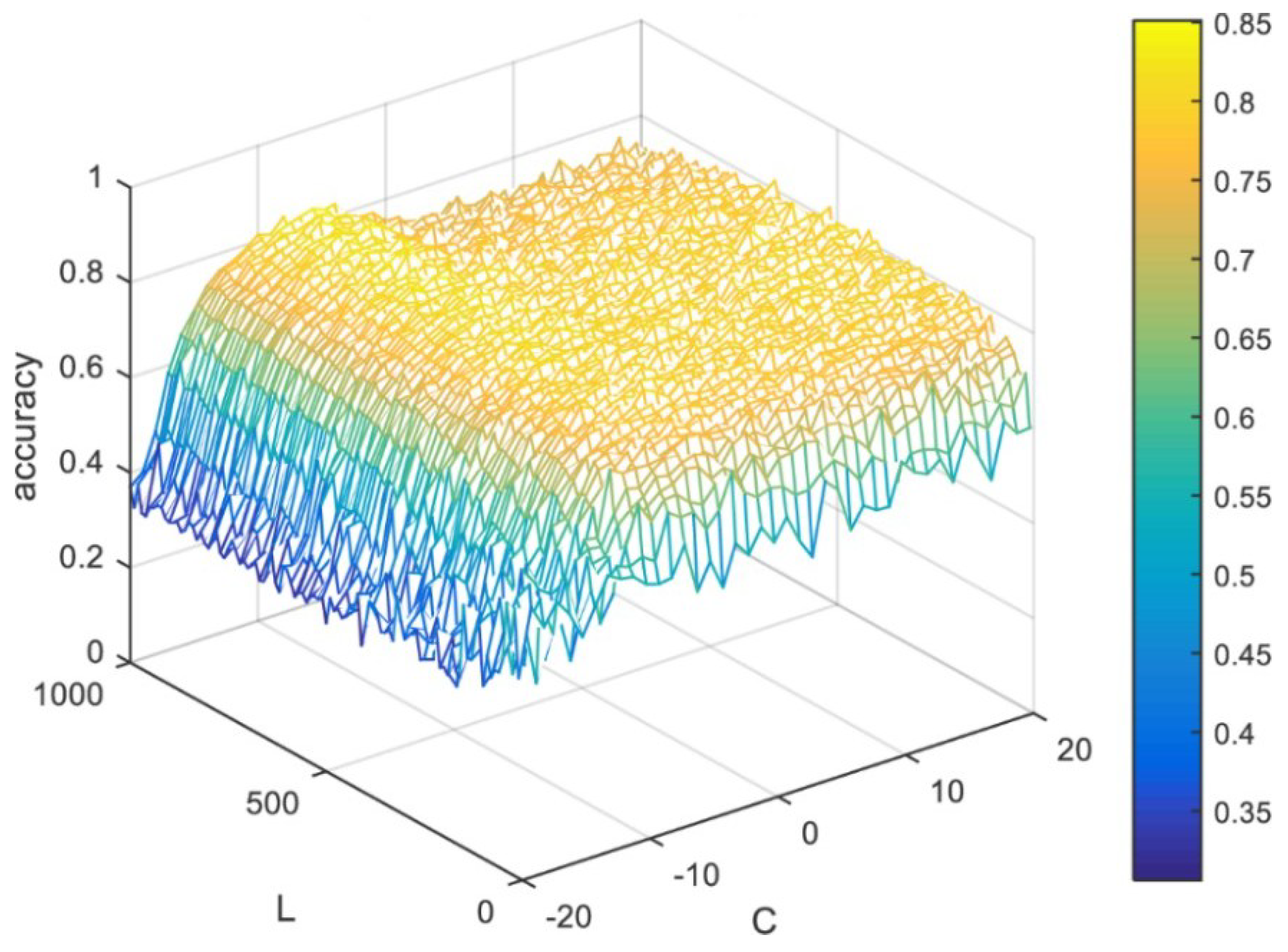
| L | Number of hidden neurons | 850 | 850 | 850 | 850 |
| Parameter Name | Parameter Description | Scenario 1 | Scenario 2 | Scenario 3 | Scenario 4 |
|---|---|---|---|---|---|
| NA | Number of features in location A | 100 | 100 | 50 | 50 |
| Number of features in location B | 50 | 50 | 100 | 100 | |
| NCF-AB | Number of Common features between locations A and B | 50 | 11 | 50 | 15 |
| L | Number of hidden neurons | 750 | 750 | 750 | 750 |
© 2019 by the authors. Licensee MDPI, Basel, Switzerland. This article is an open access article distributed under the terms and conditions of the Creative Commons Attribution (CC BY) license (http://creativecommons.org/licenses/by/4.0/).
Share and Cite
AL-Khaleefa, A.S.; Ahmad, M.R.; Isa, A.A.M.; AL-Saffar, A.; Esa, M.R.M.; Malik, R.F. MFA-OSELM Algorithm for WiFi-Based Indoor Positioning System. Information 2019, 10, 146. https://doi.org/10.3390/info10040146
AL-Khaleefa AS, Ahmad MR, Isa AAM, AL-Saffar A, Esa MRM, Malik RF. MFA-OSELM Algorithm for WiFi-Based Indoor Positioning System. Information. 2019; 10(4):146. https://doi.org/10.3390/info10040146
Chicago/Turabian StyleAL-Khaleefa, Ahmed Salih, Mohd Riduan Ahmad, Azmi Awang Md Isa, Ahmed AL-Saffar, Mona Riza Mohd Esa, and Reza Firsandaya Malik. 2019. "MFA-OSELM Algorithm for WiFi-Based Indoor Positioning System" Information 10, no. 4: 146. https://doi.org/10.3390/info10040146
APA StyleAL-Khaleefa, A. S., Ahmad, M. R., Isa, A. A. M., AL-Saffar, A., Esa, M. R. M., & Malik, R. F. (2019). MFA-OSELM Algorithm for WiFi-Based Indoor Positioning System. Information, 10(4), 146. https://doi.org/10.3390/info10040146