1. Introduction
Information system SAP is a world leader in the field of the enterprise resource planning (ERP) software and related enterprise applications. This ERP system enables customers to run their business processes, including accounting, purchase, sales, production, human resources, and finance, in an integrated environment. The running information system registers and manages simple tasks interconnected to complex business processes, users, and their activities, which are integral parts of such processes. The system provides a digital footprint of its run as it logs on more levels. When companies use such complex information systems, this software must also support their managers to have enough information for their decisions. What they can obtain from the actual information systems is usually information of quantitative types, e.g., “how many”, “how long”, “who”, “what”. Data from SAP ERP system is usually analyzed using data warehouse info cubes (OLAP technology—Online Analytical Processing). Data mining procedures also exist in SAP NetWeaver (Business warehouse, SAP Predictive Analytics), which work with such quantitative parameters. However, participants (users, vendors, customers, etc.) are connected by formal and informal relationships, and sharing their knowledge, their processes, and their behaviors can show certain common features that are not seen in hard numbers (behavior patterns). We are interested in analyzing such features, and our strategy is to analyze models using qualitative analysis with necessary domain knowledge; a similar approach can be used for the classification of unseen/new data instances.
Data received from logs contain technical parameters provided by the business process and a running information system. The goal of our work is to prepare data for management’s decision support in an intelligible format with no requirements to users for in-depth knowledge of data analysis but with the use of manager’s in-depth domain knowledge. A proper method to do this is visualization. However, visualization of a large network may suffer by the fact that such a network contains too much data and users may be misled. Subsequently, the aim is to decompose the whole into smaller, consistent parts so that they are more comprehensible and eventually (if it makes sense) repeat the decomposition. By comprehensibility, it is meant that the smaller unit more precisely describes the data it contains and its properties.
The idea to analyze process data was used already in earlier works. Authors in [
1,
2,
3] construct a social network from the process log and utilize the fact that the process logs generally contain information about users executing the process steps. Our approach is more general, as we analyze patterns in a network constructed from complex attributes.
The conversion of object-attribute representation to the network (graph) and subsequent analysis of this network is used in various recent approaches. In particular, a network is a tool that provides an understandable visualization that helps to understand the internal structure of data and to formulate hypotheses associated with further analysis, such as data clustering or classification. Bothorel et al. provide in [
4] a literature survey on attributed graphs, presenting recent research results in a uniform way, characterizing the main existing clustering methods and highlighting their conceptual differences. All the aspects mentioned in this article highlight different levels of increasing complexity that must be taken into account when various sets and number of attributes are considered due to network construction. Liu et al. in [
5] present a system called Ploceus that offers a general approach for performing multidimensional and multilevel network-based visual analysis on multivariate tabular data. The presented system supports flexible construction and transformation of networks through a direct manipulation interface and integrates dynamic network manipulation with visual exploration. In [
6], van den Elzen and Jarke J. van Wijk focus on exploration and analysis of the network topology based on the multivariate data. This approach tightly couples structural and multivariate analysis. In general, the basic problem of using attributes due network construction from tabular data is finding a way to retain the essential properties of transformed data. There are some simple methods often based on ε-radius and k-nearest neighbors. One of the known and well working approaches based on the nearest neighbor analysis was published by Huttenhower et al. in [
7]. In this approach, in addition to the graph construction, the main objective is to find strongly interconnected clusters in the data. However, the method assumes that the user must specify the number of nearest neighbors with which the algorithm works. Methods using the principle based on the use of k-nearest neighbors are referred to as the k-NN networks and assume the k parameter to be a previously known value.
In our approach, we use the LRNet algorithm published by Ochodkova et al. [
8]. This method is also based on the nearest neighbor analysis; however, it uses a different number of neighbors for different nodes. The number of neighbors is based on analysis of representativeness as described by Zehnalova et al. in [
9]. In comparison with other network construction methods, the LRNet method does not use any parameter for the construction except a similarity measure. Moreover, networks resulting from the application of the LRNet method have properties observed in real-world networks, e.g., small-world and scale-freeness.
This work formulates and develops a methodology that covers selecting a proper log from the SAP application, data integration, pre-processing and transformation, data and network mining with the following interpretation and decision support. Real data and network analysis from the experiment is presented in
Appendix A.
2. Materials and Methods
The first group of methods covers the transformation of logs from the real SAP business process run into the Object–Attribute table/vector. This group of methods contains a selection of proper logs and their integration, pre-processing, and transformation.
- ○
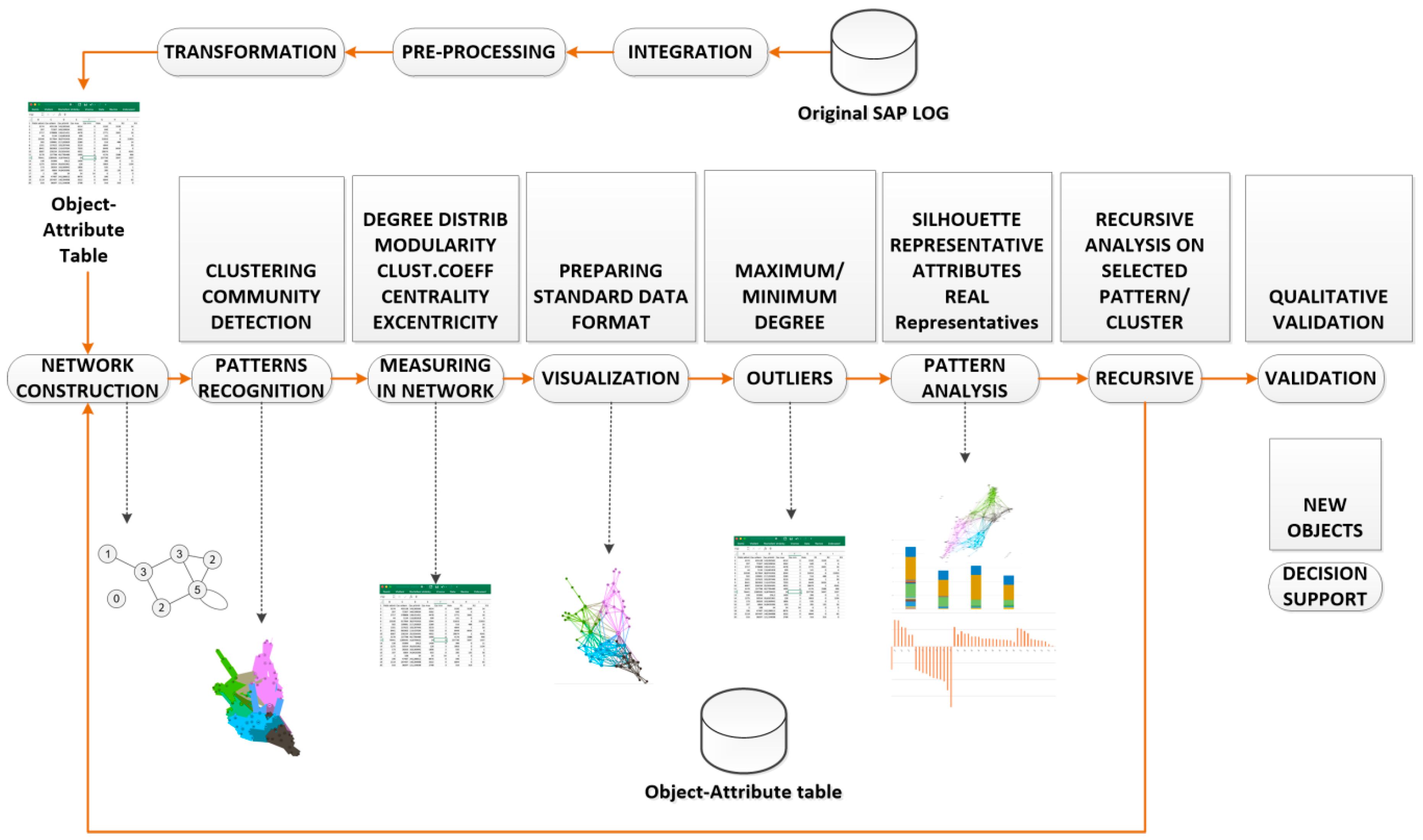
Integration. The proper logs and methods of change documents are selected—there are several in log sources in SAP systems, usually more of them are used as a data source for the original SAP LOG shown in
Figure 1. A list of the most often used data LOG sources is presented in
Appendix A.
- ○
Pre-processing uses several procedures described in
Section 3.1 (cleaning, extension, anonymization).
- ○
Transformation generates final Object–Attribute table as is described in
Section 3.1.
Core data of logging is based on the Case–Event principle. The case represents one complete pass of the process, and the event represents one step/activity related to the specific case. The requested object for the following analysis is selected (objects user, vendor, invoice participating in the process of vendor invoice verification). Attributes of the analyzed objects are selected from the source log, and new attributes are defined (and calculated) that can help to describe the objects’ behavior. The final anonymized and normalized Object–Attribute table for the next data mining analysis is prepared.
The transformation of the Object–Attribute table into a network and community detection is done following used methods. As mentioned above, we use the LRNet [
8] algorithm by utilizing local representativeness for the vector–network transformation and the Louvain method of community detection [
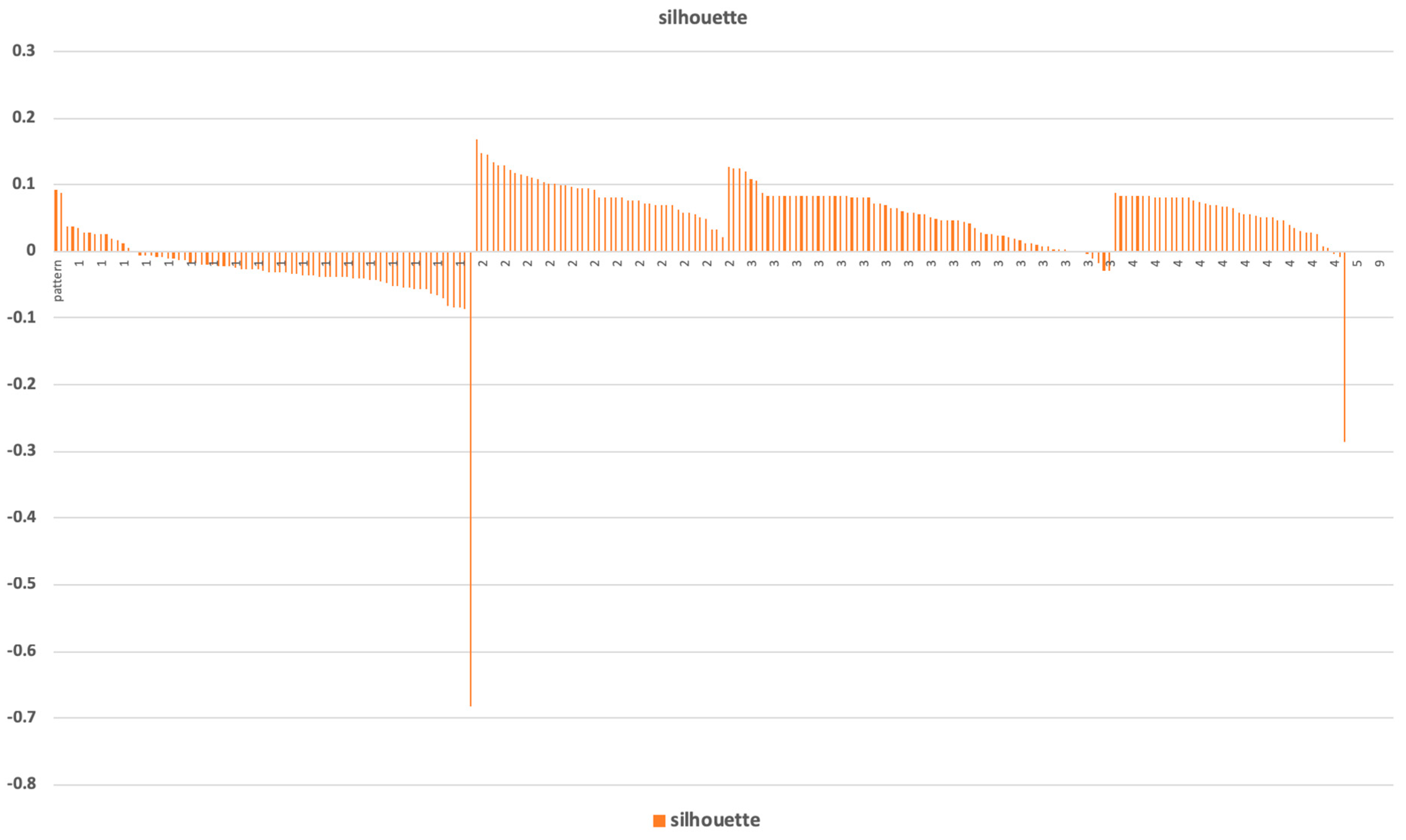
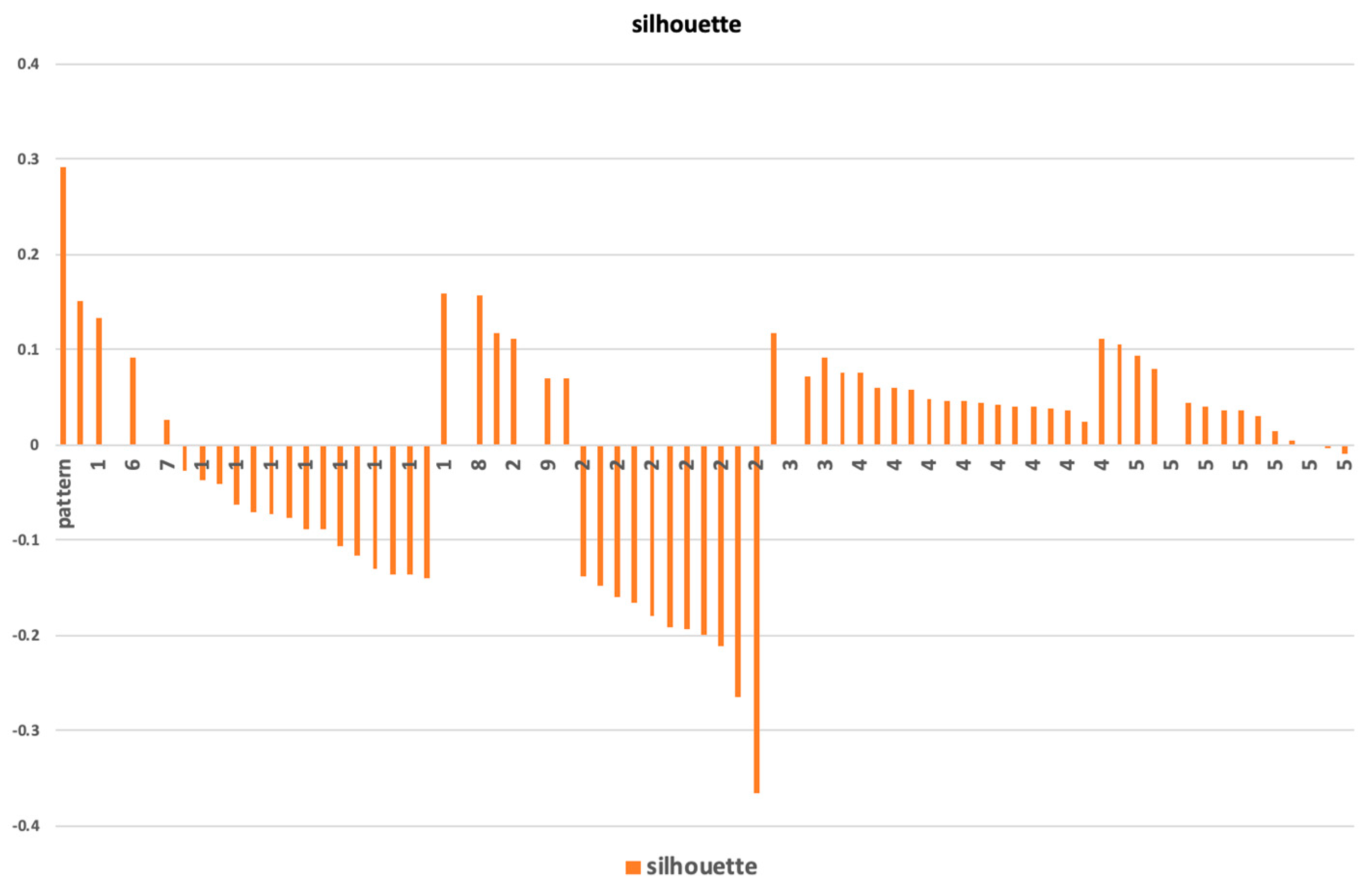
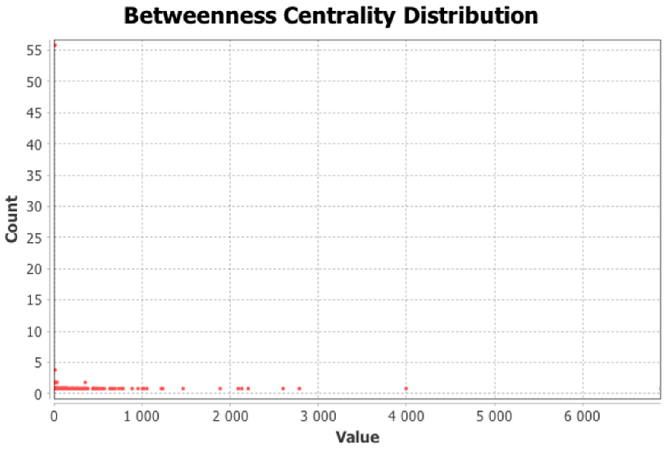
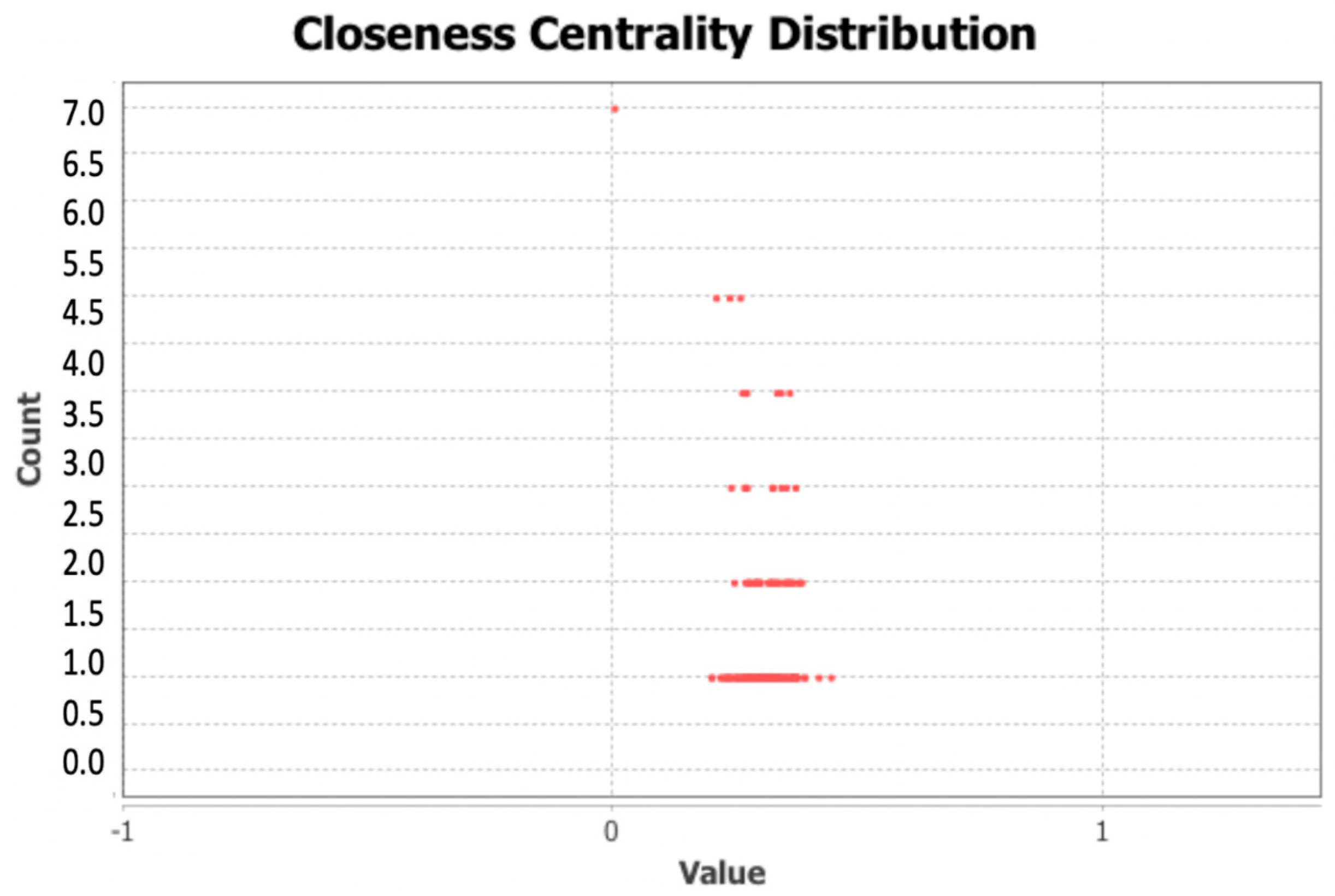
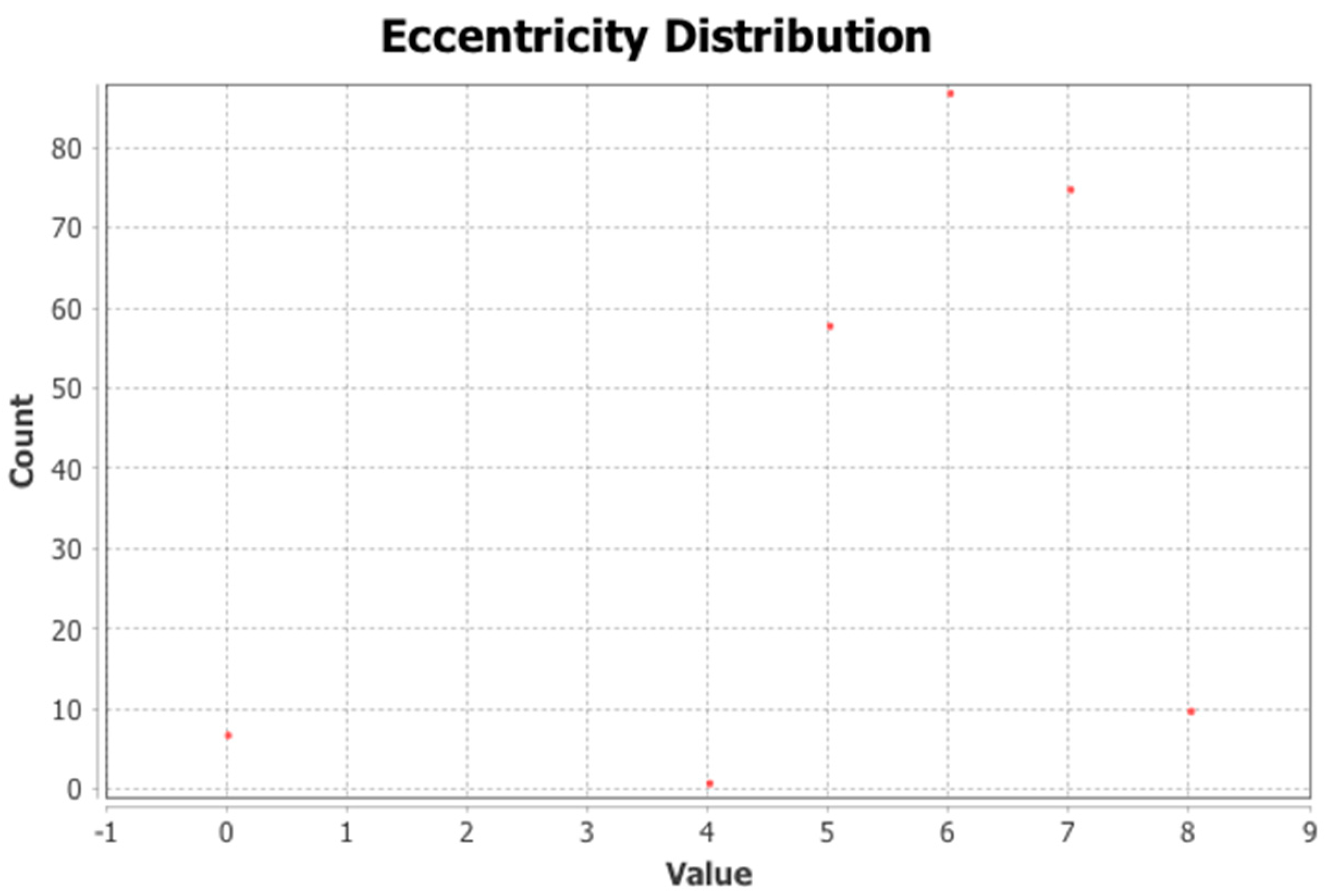
10]. The network and the detected communities are measured and analyzed. Visualization provides a fast user-accepting tool for recognition of specific situations and relations in the network. We utilize several network measures that we use for analyzing network parameters and communities—silhouette (the quality of clustering), modularity (a potential for division into communities), and centralities (eccentricity distribution). We identify two types of outliers, network outliers and attribute outliers.
Communities are identified as we showed above. Common characteristics of the nodes of specific communities are considered as patterns. Every pattern provides information containing a combination of value mix of profile attributes. We apply methods of statistical analysis to these patterns’ attributes. This mix of values for all the patterns provides a model. A representative participant can be found for each pattern (vector of attributes calculated as the average of relevant attributes of all cluster participants). The analysis is performed for the participants similarly with a representative on one side and typically non-conforming participants of the cluster on the other side. The participants can be distributed by their conformity with the model attributes.
The found communities are assessed, and communities with suitable parameters are used for decomposition. A recursive analysis is run on all identified clusters when average silhouette and modularity of detected clusters are high. In a case where the average silhouette of clusters is near zero or negative, we do not continue with the recursive analysis. The process, starting with network construction and ending with decomposition, is schematically described in
Figure 1.
We use a qualitative validation and an interpretation based on domain knowledge. Evaluation of patterns, communities, and outliers in the real organization environment provides a validation of the found results. As we dispose of all information about source objects and relations with knowledge about the original environment, we prepare an interpretation of the received model and its patterns.
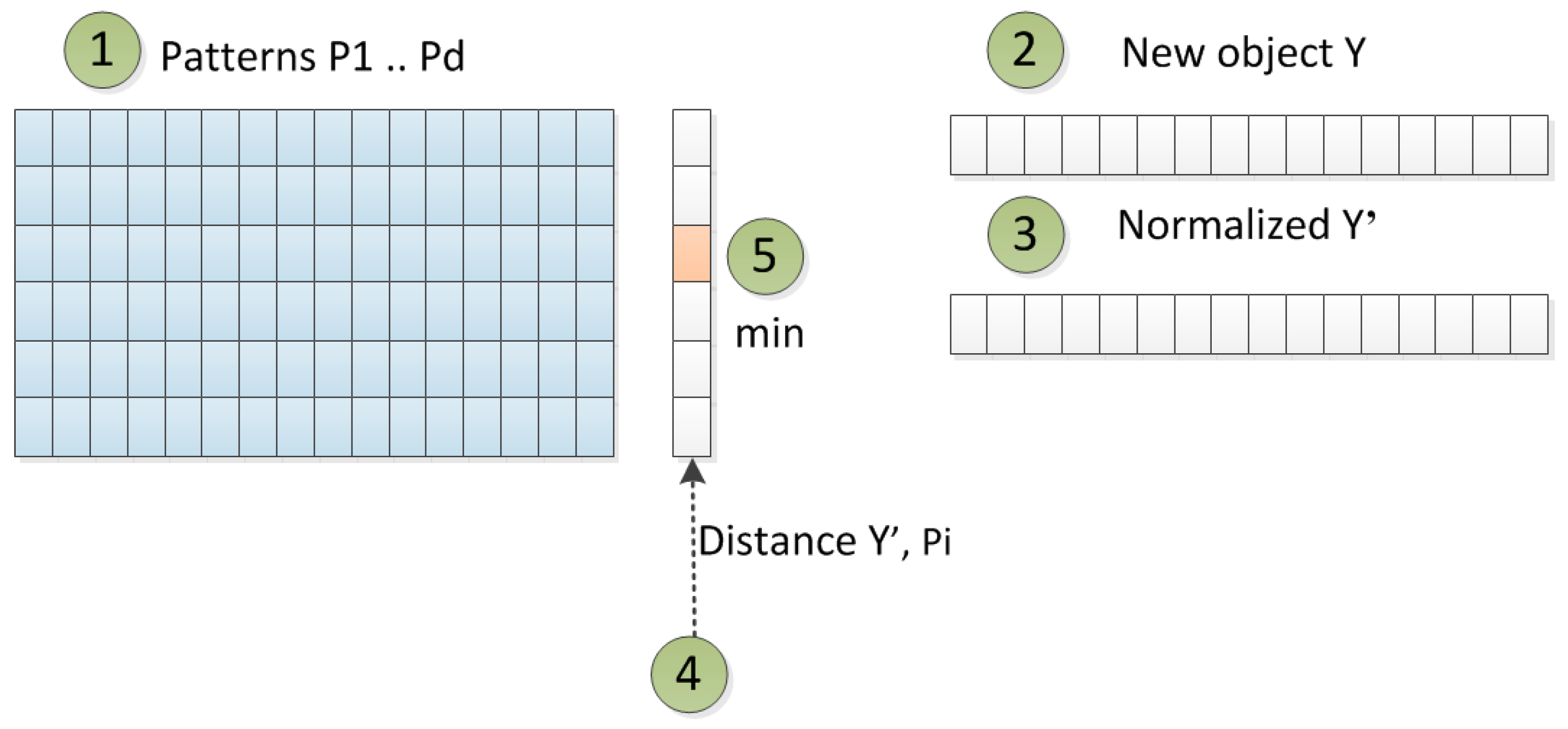
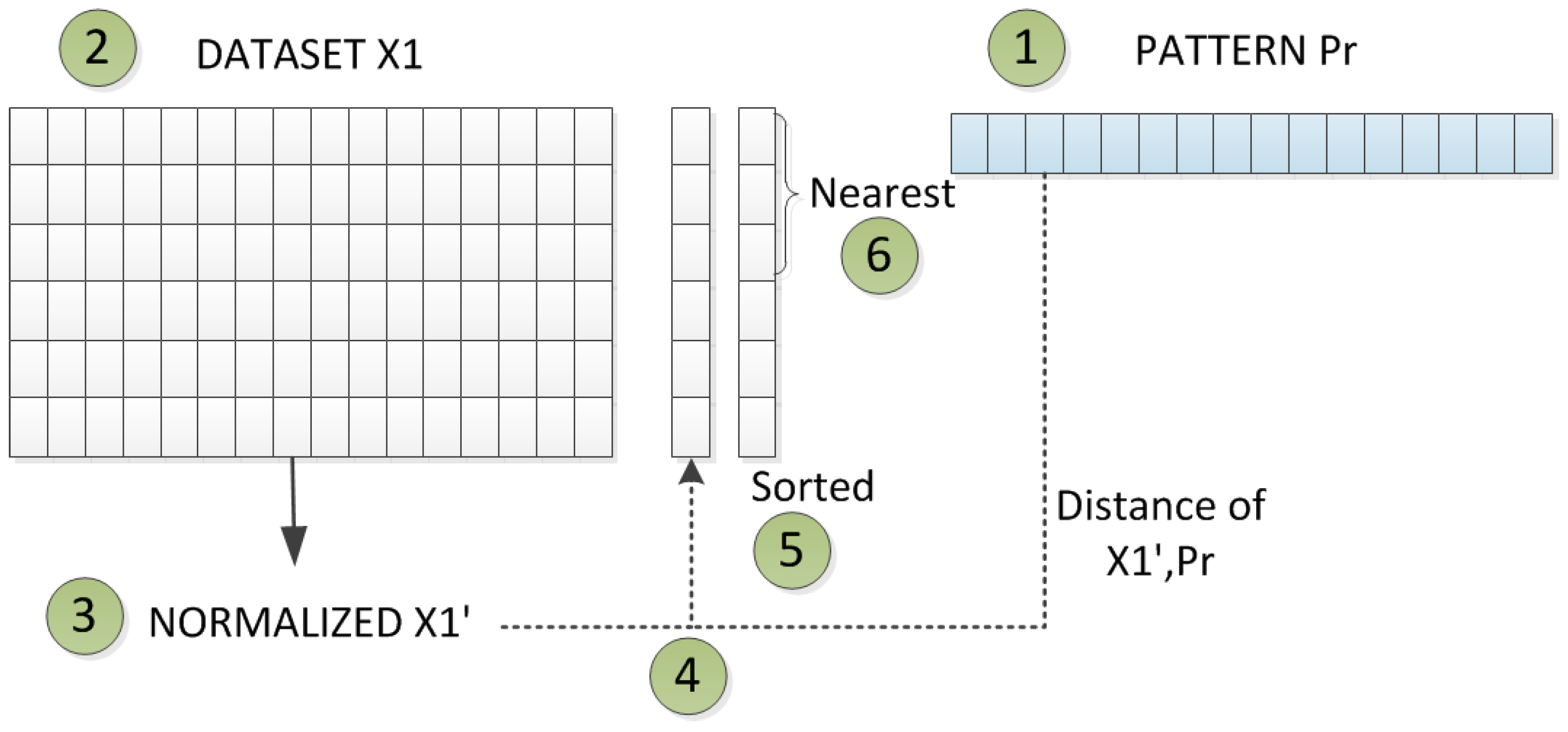
We work with a method of manual qualitative validation for decision support, and results from data mining are compared with the real environment of running business processes. This qualitative assessment serves as verification of results from data mining. It uses identified patterns from the original dataset. When a new object appears, we can compare this object with all identified patterns and find the most fitting pattern for the new object. Then, a comparison of attributes can be performed, and it can be analyzed if the behavior of a new object also fits the behavior of the found pattern. Another kind of qualitative validation is performed for finding the original records for the pattern for an extended/reduced original dataset.
The pre-processed log is prepared in the Object–Attribute format, where attributes are prepared into a numerical format. We use the Euclidean distance for a similarity function to measure the similarity more easily. The issue is that data in a vector format in high dimension cannot be effectively visualized. As much as we would like to visualize the data and results for managers, we decide to transform the initial Object–Attribute table into a network.
4. Discussion
We presented the methodology of knowledge discovery from data that we used for data mining of logs generated from the SAP systems. Using this approach, we analyzed a specific business process (invoice verification) from the specific real environment, as was described in
Section 3. We showed how the network was constructed, how patterns were found, and how they can be visualized and analyzed recursively.
The used method of network construction with following community detection has some known limitations in complexity; used algorithms have quadratic complexity O(n2) for the network construction, which is done by the representativeness computing. From this perspective, the method can be used for samples with limited size. On the other hand, for business processes with several hundred thousands of activities, the method works in an order of seconds and is still usable.
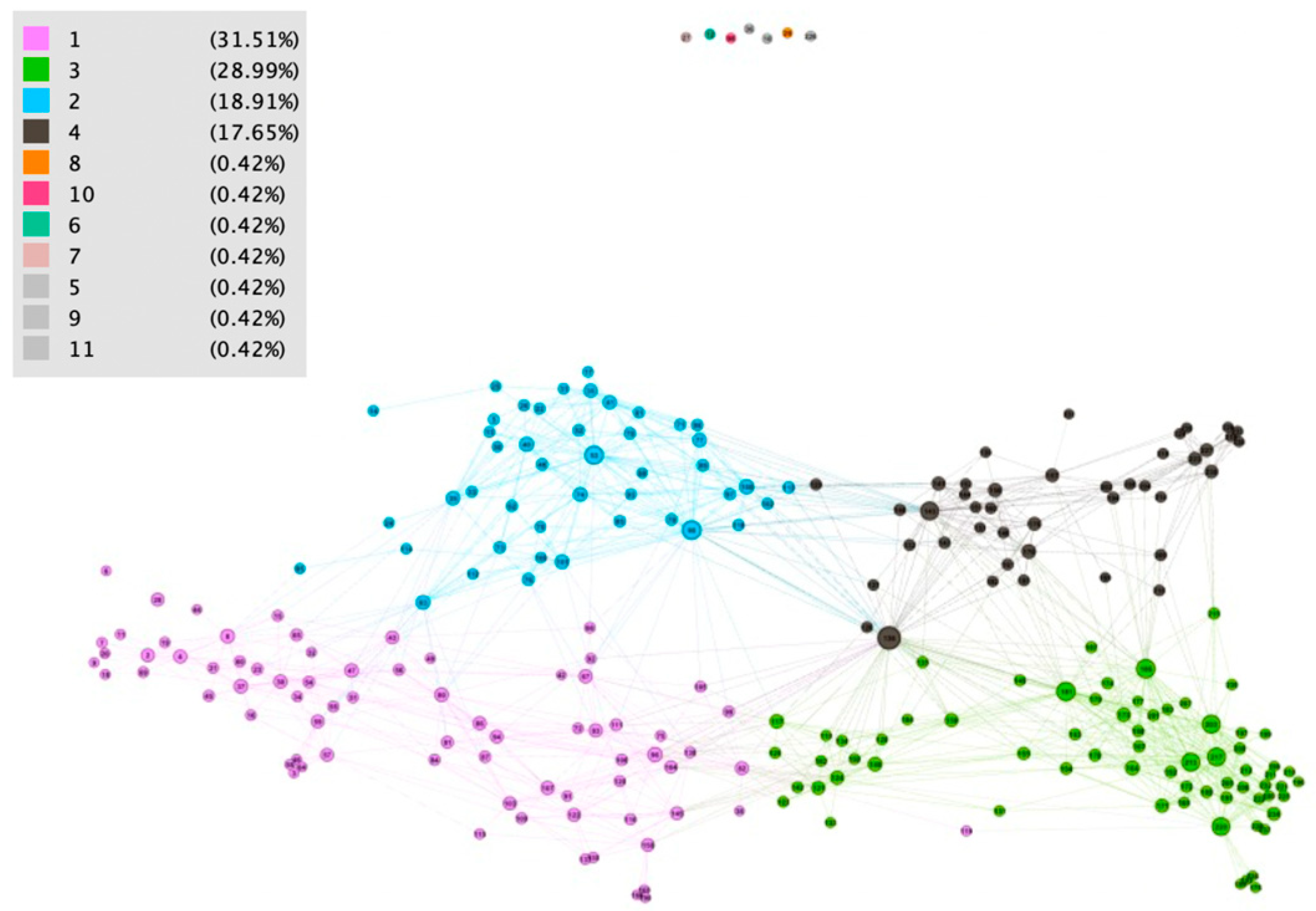
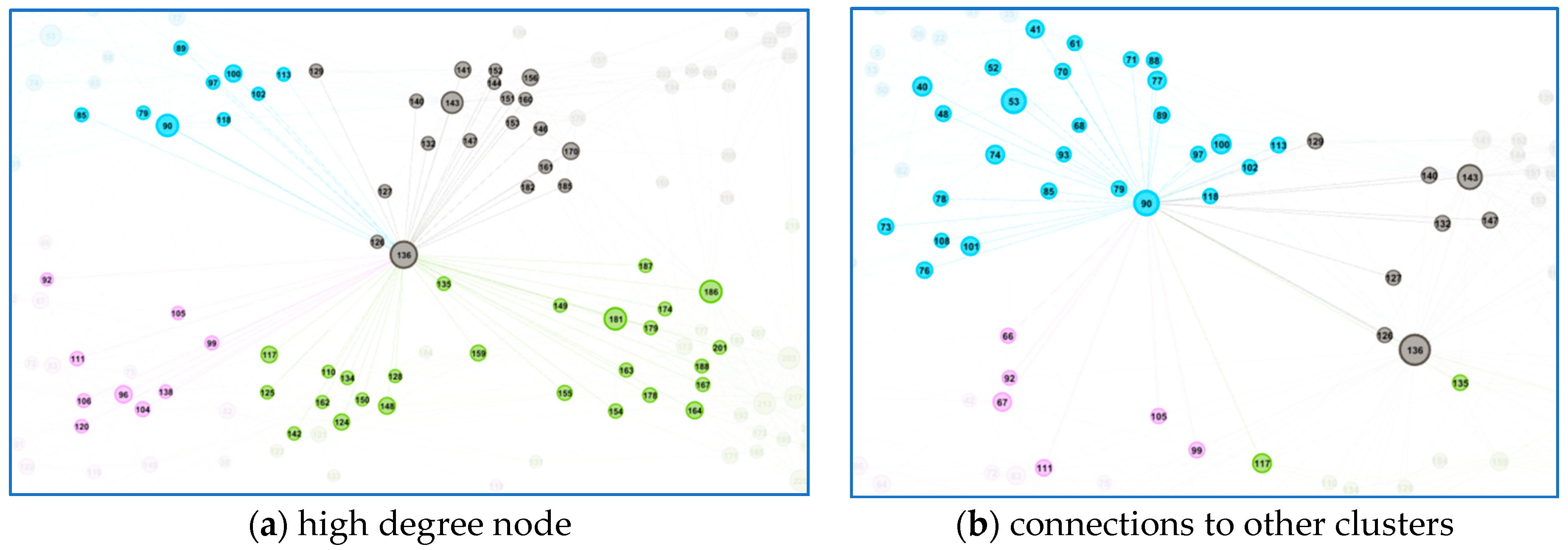
Another discussion was about visualization. We selected two dimensional visualization of the network to focus users with several factors—a local characteristic (node degree) was represented by the size of the node, and a network characteristic (community structure) was represented by the density of vertices in between the community. As managers prefer to accept a more straightforward message, improving the visualization method is still open for future work.
We also analyzed users with the high (or highest) degree. It turned out that such users were also interconnected with neighbor clusters and they were not typical clusters representatives. We identified types of such users, but no specific common behavior was found for high-degree users.
We can say that this method of network analysis identified a set of communities and a set of network outliers from a given data set. It was important to identify both kinds of sets. In our article, the network outliers were analyzed in
Table 5 and
Table 7, the pattern of found communities were described in
Figure 6,
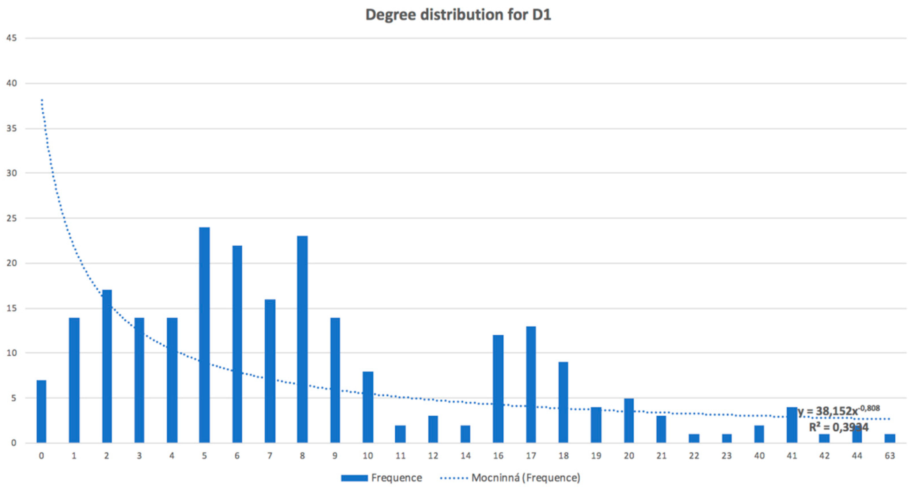
Table 6 displays data source
D1, and
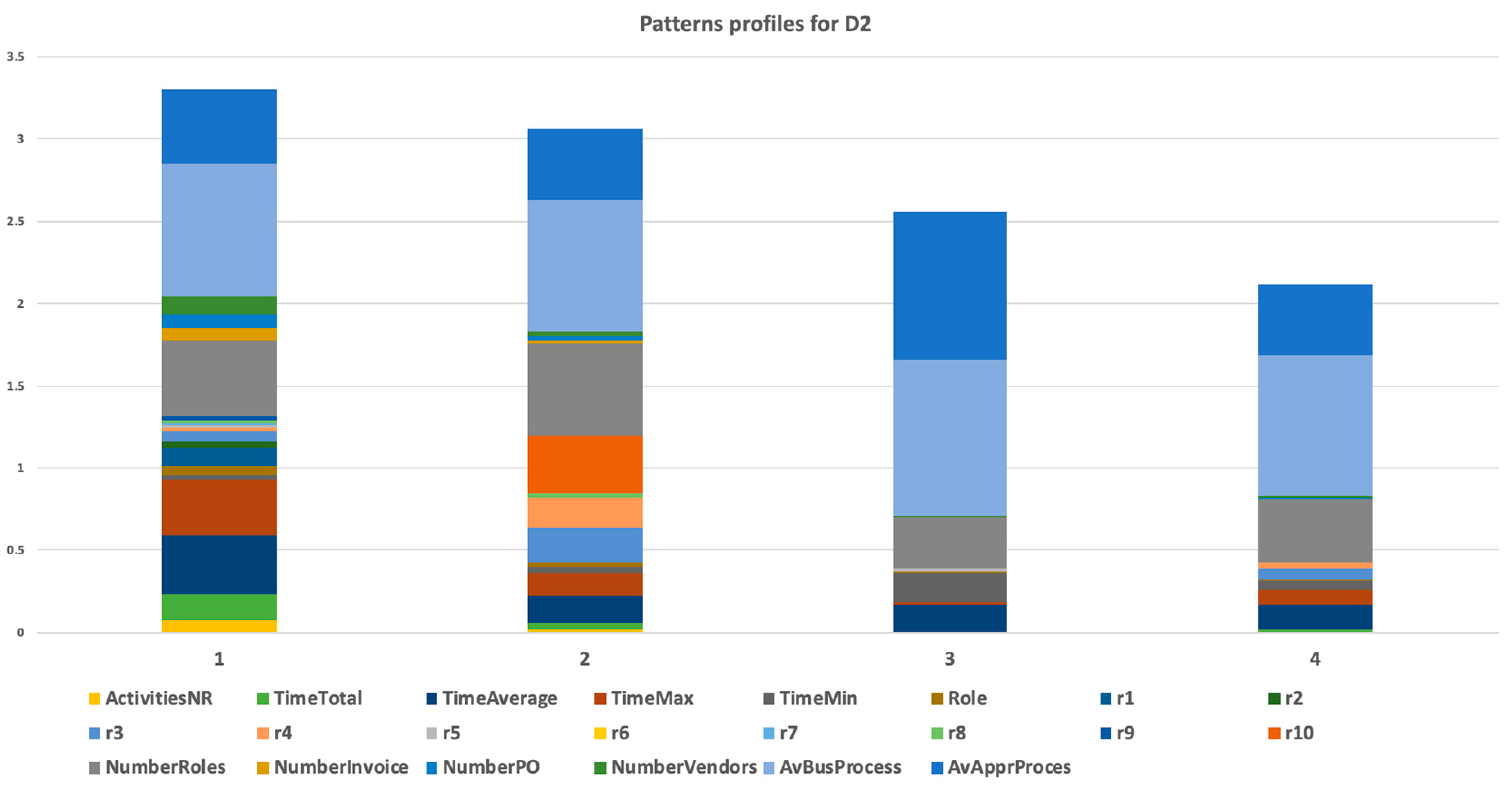
Figure 11 and
Table 8 show data source
D2. The finding should be taken back to the real implementation environment and manager or consultant with domain knowledge should identify what the significance or character of the outlier/pattern is. Specifically, we identified seven network outliers for data source
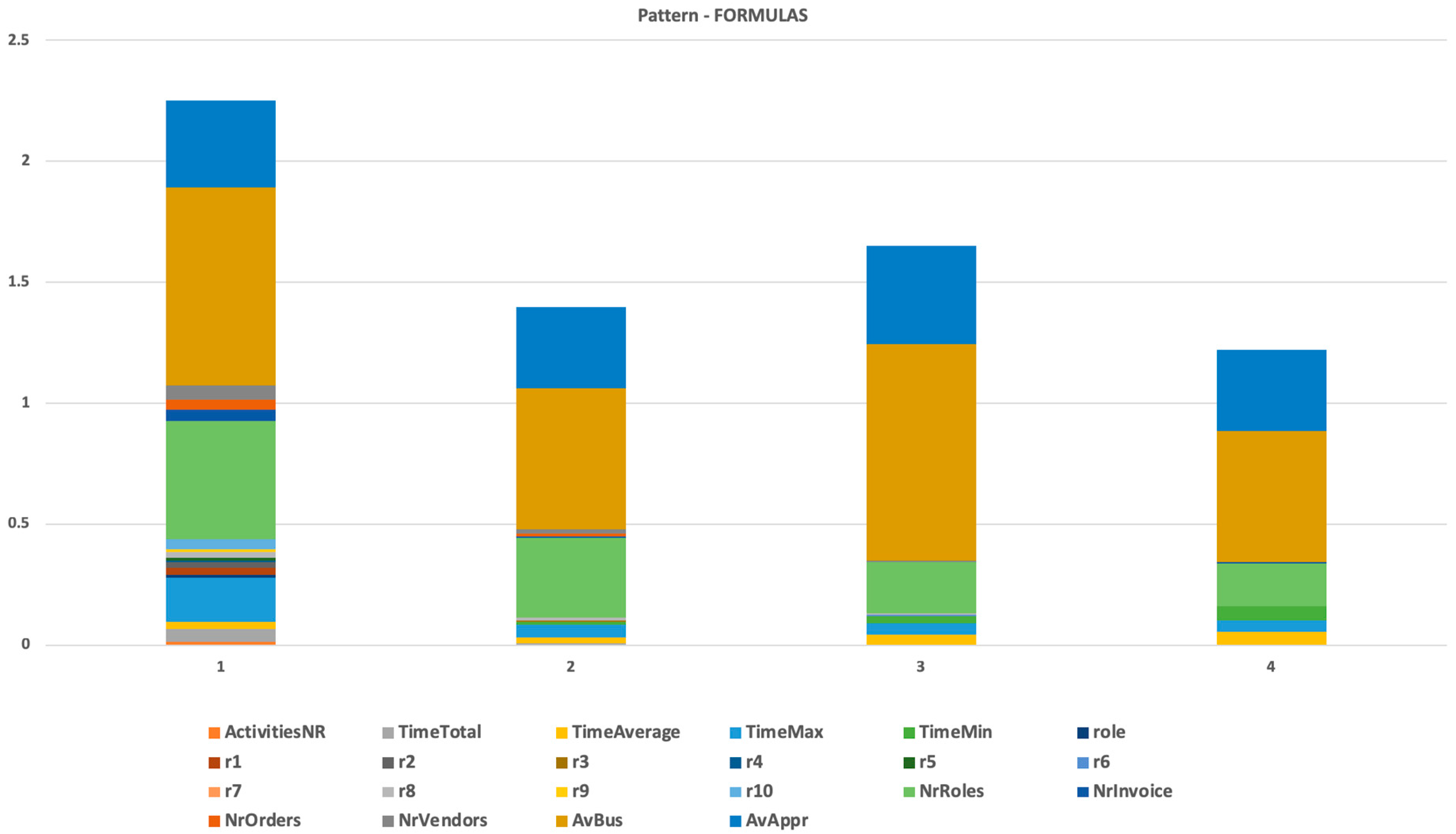
D1, where five of them (11, 10, 8, 6, and 7) were special users, and we understood that they were outliers for this reason; two of them (5 and 9) should be analyzed in detail, because they had different behaviors than other users from their department. Our method revealed specific users that had different behaviors that were typical in a set of users with a similar organizational assignment. The other discussion could be about network patterns. We identified four communities (described by patterns) for data set
D1. As was described in
Section 3.2.2, domain knowledge could be used for the specification of attribute values mix. For example, pattern 1 represented users processing invoices of regular vendors with many regular orders. What could have been significant was if in the extended dataset, some regular vendor had its invoice verification process in other cluster/pattern. It could certainly be done by outbalancing another attribute, but this should be analyzed.
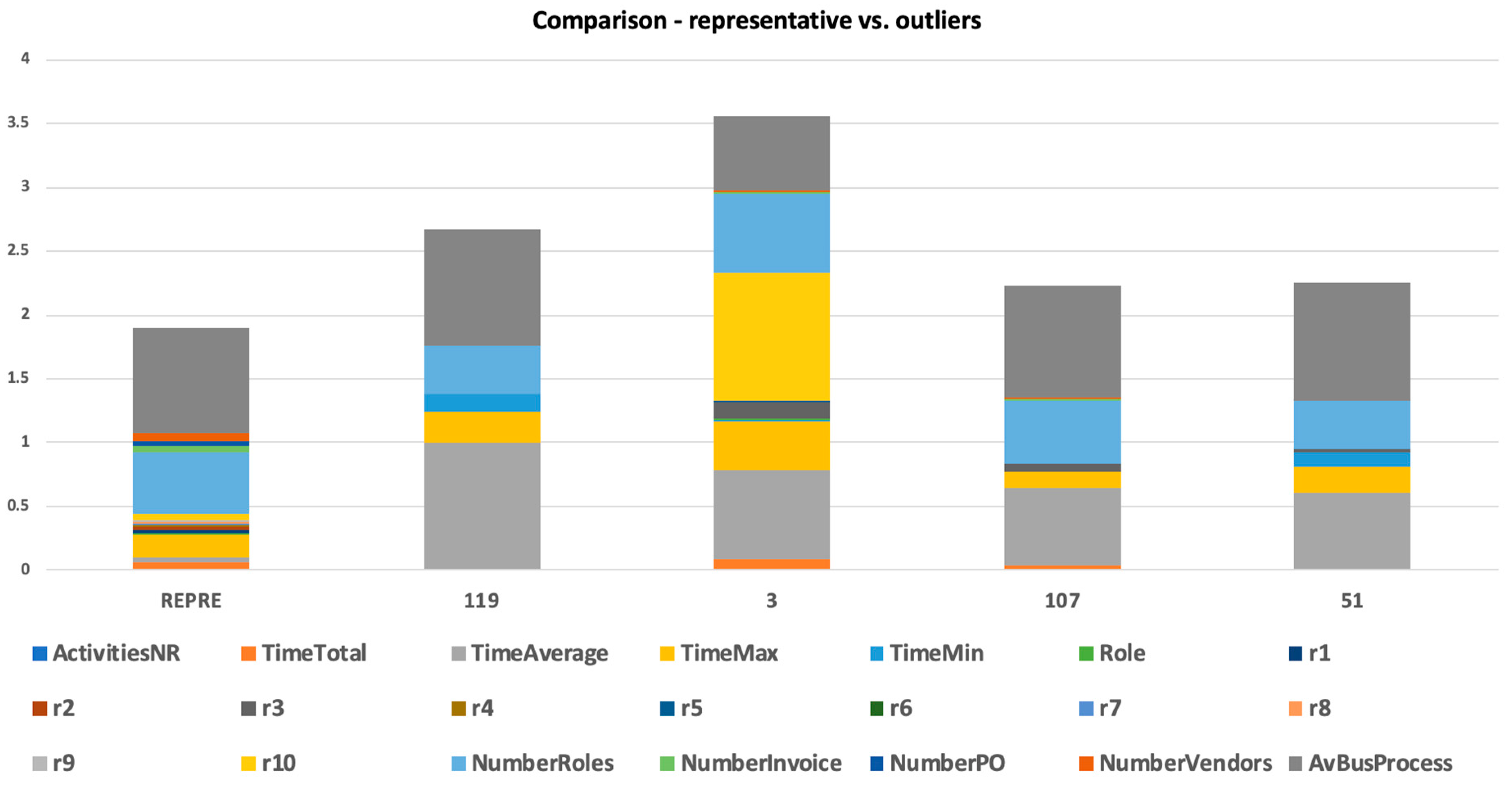
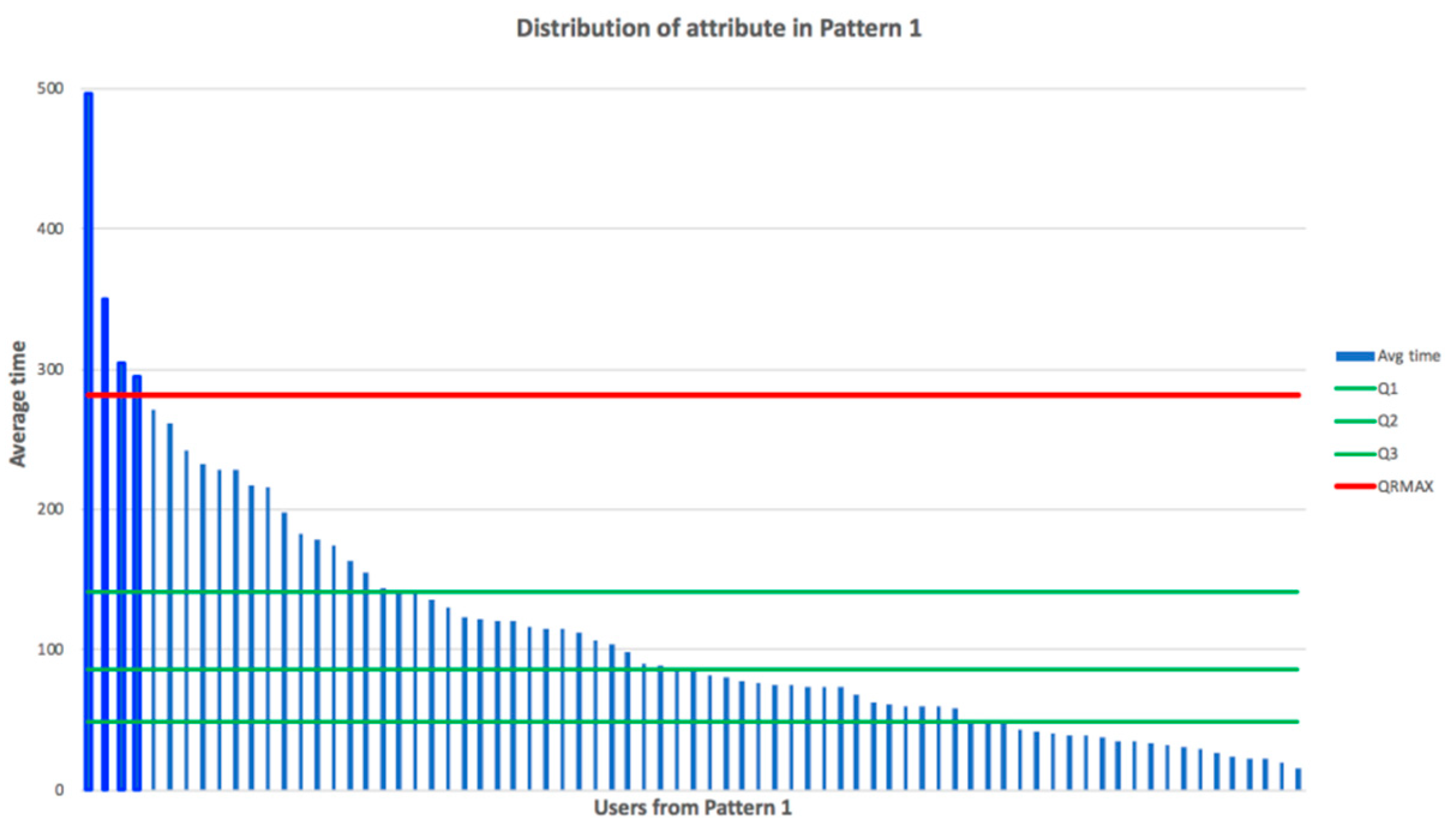
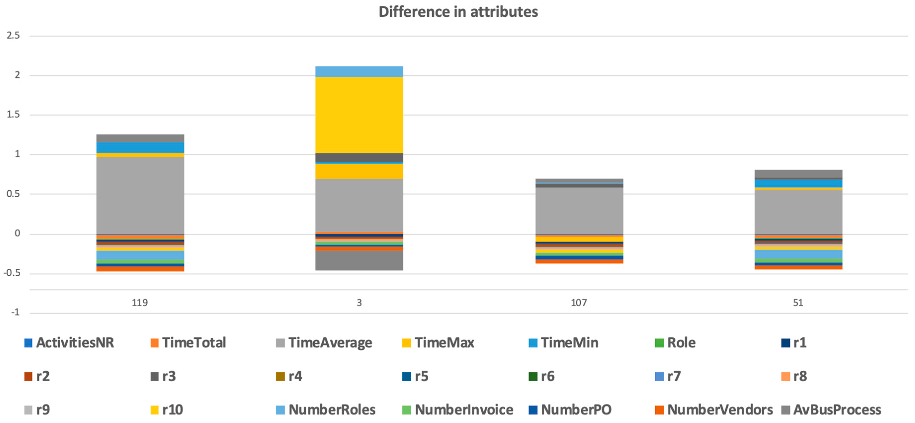
Every cluster pattern was calculated using a vector of attributes. We could focus on some attribute and see the distribution of the cluster participants based on such attribute, as we showed in
Figure 7. We could see the outliers of this cluster (with a focus on selected attribute). We could visualize how these outliers differed in selected attributes and in a mix of attributes (
Figure 8 and
Figure 9).
The methodology contains steps for analyzing patterns in the real environment and running a recursive analysis of interesting patterns (e.g., unstable patterns or patterns with apparent exceptional participants, which could be a participant “far” from the representativeness of the pattern). The border of recursive processing of specific patterns could also be discussed. Our approach was to run recursive analysis while average silhouette and modularity of detected clusters were high. In a case where the average silhouette of clusters was near zero or negative, we did not continue with the recursive analysis.
We proved that the approach uncovered some patterns by found representativeness parameters that are typically present on this business process (number of roles, average time, etc.).
Another contribution is the finding that the pattern (as a combination of representativeness) can be used as a model for:
- ○
decision support for an assignment of a new object to an existing pattern with a possible comparison of representative attributes and the real behavior in an organization;
- ○
searching back to the original dataset or to a reduced/extended dataset (in this case, we suggest using only representative attributes) for showing the pattern representatives more quickly and for detailed inspection, which was proven back on the real datasets.


