Article

A Modified Robust FCM Model with Spatial Constraints for Brain MR Image Segmentation

1
School of Physics and Information Engineering, Minnan Normal University, Zhangzhou 363000, China
2
School of Electronic Engineering, Heilongjiang University, Harbin 150080, China
*
Author to whom correspondence should be addressed.
Information 2019, 10(2), 74; https://doi.org/10.3390/info10020074
Submission received: 19 January 2019 / Revised: 13 February 2019 / Accepted: 19 February 2019 / Published: 21 February 2019
(This article belongs to the Special Issue eHealth and Artificial Intelligence)

Abstract

:
In brain magnetic resonance (MR) images, image quality is often degraded due to the influence of noise and outliers, which brings some difficulties for doctors to segment and extract brain tissue accurately. In this paper, a modified robust fuzzy c-means (MRFCM) algorithm for brain MR image segmentation is proposed. According to the gray level information of the pixels in the local neighborhood, the deviation values of each adjacent pixel are calculated in kernel space based on their median value, and the normalized adaptive weighted measure of each pixel is obtained. Both impulse noise and Gaussian noise in the image can be effectively suppressed, and the detail and edge information of the brain MR image can be better preserved. At the same time, the gray histogram is used to replace single pixel during the clustering process. The results of segmentation of MRFCM are compared with the state-of-the-art algorithms based on fuzzy clustering, and the proposed algorithm has the stronger anti-noise property, better robustness to various noises and higher segmentation accuracy.

1. Introduction

Magnetic resonance imaging (MRI) has been widely used in clinical diagnosis because of its advantages of non-ionizing radiation and wide applicability. In order to detect the volume change of brain tissue in physiological or pathological state [1], doctors often need to segment the brain MR images accurately. Generally, the MR images are divided into white matter (WM), gray matter (GM) and cerebrospinal fluid (CSF), which can quantitatively measure the cross-sectional area or volume of brain tissue or lesions to improve the accuracy of the diagnosis of patients’ condition. Therefore, the visual quality of MR images directly affects the accuracy of clinical diagnosis. However, the acquisition of MR images may be affected by noise, resulting in serious degradation of image quality, which brings some troubles for the accurate segmentation of brain tissue.
At present, there are many segmentation methods for brain MR image, such as threshold method [2], region method [3], random field method [4], neural network method [5] and clustering method [6,7,8,9]. As one of the main techniques of unsupervised machine learning, clustering method, especially fuzzy c-means (FCM) clustering method [10], has been widely used in brain MR image segmentation. But unfortunately, although the standard FCM algorithm works well on noise-free images, it is very sensitive to noise and other disturbances in the image because it does not consider any spatial neighborhood information. In order to overcome this disadvantage of FCM, the corresponding image preprocessing schemes were presented in some literature [11,12,13,14,15,16], and then FCM algorithm was used. Pedrycz et al. [11] took advantage of the available classified information and actively applied it as part of their optimization procedures. Szilagyi et al. [12] proposed an enhanced fuzzy c-means clustering (EnFCM) algorithm to accelerate the image segmentation process. In EnFCM, the pixels of an image are replaced by their gray-level histogram, and the statistical number and calculation is much smaller than FCM. In order to further reduce the computational time and improve the parameter inflexibility, Cai et al. [13] presented a fast generalized fuzzy c-means clustering (FGFCM) method, and FGFCM introduced a flexible locality factor Sij incorporating simultaneously both the gray-level difference and spatial distance in a local window. Ahmed et al. [16] proposed an adaptively regularized kernel-based fuzzy c-means clustering (ARKFCM) algorithm for brain MR image segmentation. ARKFCM employed the heterogeneity of grayscales in the neighborhood and exploited a measure for local contextual information to replace the standard Euclidean distance with Gaussian radial basis kernel functions. However, in these methods, some important details in the image may be lost due to the use of an image smoothing operation, especially boundary or edge. In addition, they are difficult to control and adjust the balance between smooth and non-smooth clustering. To mitigate the effects of noise in brain MR images, a fast image segmentation algorithm based on FCM clustering is proposed in this paper, it does not require a balance control factor, and the related parameters can be adaptively acquired from local neighborhood information. MRFCM algorithm can improve the robustness against noise and program execution efficiency.
The remaining of this paper is organized as follows. Several well-known models are briefly described in Section 2. The proposed model MRFCM is introduced in detail in Section 3. The comparison results of MRFCM with several state-of-the-art models and quantitative evaluation are demonstrated in Section 4 to show the performance of MRFCM. Finally, we give the conclusion of this paper in Section 5.

2. Basic Concepts and Related Algorithms

2.1. Enhanced FCM

In view of the shortcomings of the standard FCM algorithm being sensitive to noise, the improved FCM algorithm introduced by Ahmed et al. [17] adopted cyclic optimization filtering, which improved the image segmentation quality. However, due to the addition of loop iteration in the convergence, the algorithm was inefficient and ran for a long time. Therefore, Szilagyi et al. [12] proposed an Enhanced FCM (EnFCM) algorithm, which effectively improved the computational efficiency in the segmentation process and also provided higher segmentation quality for MR brain image. In order to speed up the image clustering, a linear weighted sum was formed in advance from the original image and its local spatial neighborhood in EnFCM, as follows
ξ i = 1 1 + α ( x i + α N R j N i x j )
where ξi is the linear weighted gray value of the ith pixel in the image, the parameter α is used to adjust the intensity of the neighborhood constraint, xj is the gray value of neighborhood pixels centered at xi, and NR denotes the pixel number of neighborhood pixels. In fact, ( j N i x j ) / N R represents the mean filtering of pixels in the neighborhood. During the running of the program, each pixel in the image is not directly calculated, but the linear weighted sum in Equation (1) is clustered. The objective function of EnFCM algorithm is
J E n F C M = k = 1 c l = 1 q γ l u k l m ( ξ l v k ) 2
where vk is the kth cluster center, ukl represents the fuzzy membership of the kth cluster that gray value is l, and q denotes the number of gray levels of a given image, q is much less than the total number N of image pixels. γl denotes the number that gray value of the pixel is equal to l, satisfying
l = 1 q γ l = N
Under the constraints of k = 1 c u k l = 1 for any gray value l, the partial derivatives of JEnFCM to ukl and vk are solved by using Lagrange optimal criterion to minimize respectively, then the updated expressions of corresponding fuzzy membership and cluster center are
u k l = ( ξ l v k ) 2 m 1 j = 1 c ( ξ l v j ) 2 m 1
v k = l = 1 q γ l u k l m ξ l l = 1 q γ l u k l m .
There are generally 256 gray levels per pixel in brain MR image, which is much smaller than the total number of pixels in the image. It can be seen from Equations (4) and (5) that the running time of EnFCM program is significantly reduced. EnFCM provides a fast and robust segmentation method, but the quality of the segmentation result depends largely on the control factor α, the size of the neighborhood region and other parameters. If the parameter α is set to be large enough, the anti-noise ability will be improved, but the boundaries or details may be lost. On the other hand, if the parameter α is sufficiently small, although the segmented image can retain more detail information, the sensitivity to noise is increased. Therefore, there is no prior knowledge about image noise, the choice of parameter α is a difficult task. In general, it can only be decided as an optimal value by trial-and-error.

2.2. Fast Generalized FCM

In order to avoid the selecting problem of the parameter α and improve the clustering effect, Cai et al. [13] proposed a fast generalized fuzzy c-means clustering (FGFCM) algorithm. FGFCM introduced a local similarity measure Sij containing grayscale and distance information, which is defined as follows
S i j = { e max ( | p i p j | , | q i q j | ) / λ s x i x j 2 / λ g σ i 2 , i j 0 , i = j .
Let xi is the gray value of center pixel in the local window, xj denotes the gray value of neighbor pixel falling into window, (pi, qi) denotes the position coordinate of pixel xi in the image, λs and λg are two scale factors, they have a similar functionality with α in EnFCM, and σi is defined as
σ i = j N i x i x j 2 N R
where NR represents the number of pixels in the neighborhood. In FGFCM, the similarity measure Sij is used to calculate the new gray value ξi, and a new image ξ is obtained as follows
ξ i = j N i S i j x j j N i S i j .
Compared with EnFCM, FGFCM can improve the segmentation accuracy, and the parameter Sij can be changed with the change of local neighborhood window, which overcomes the defect of fixed parameter α to some extent and has better flexibility.

3. Basic Principles of The Modified Algorithm

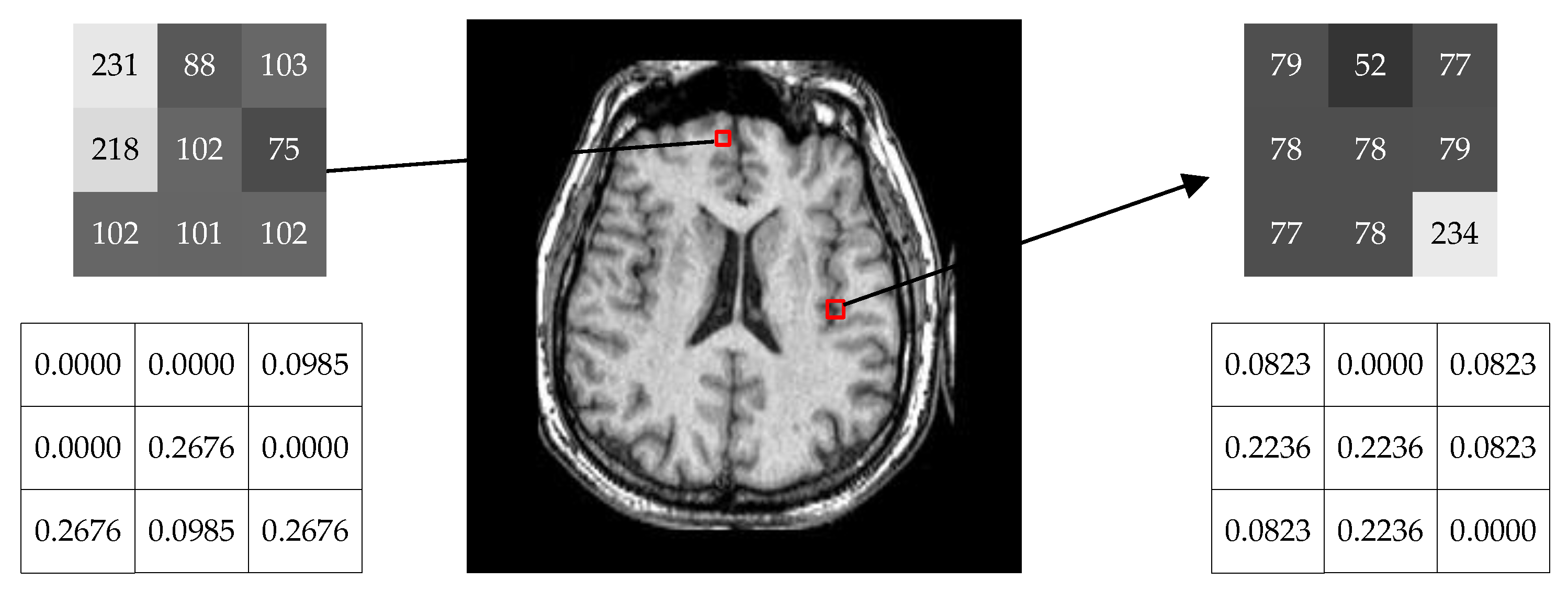
3.1. Weighted Measure with Neighborhood Information

There are usually two kinds of common noise in the image: pulse-like noise and Gaussian noise. Since the generation mechanisms and expressions of two types of noise are very different, it is difficult to design an algorithm which can effectively remove two kinds of noise at the same time. The classical median filter is very effective for impulsive noise, but it does not perform well for Gaussian noise. Mean filter is good for eliminating Gaussian noise, but it is very poor for impulsive noise. Therefore, in order to overcome the influence of noise using FCM algorithm to segment noisy images, based on the EnFCM, FGFCM and ARKFCM algorithm [16], a modified image segmentation algorithm with spatial constraints is proposed for noisy image in this section.
Firstly, let data set X = {x1, x2, …, xn} be composed of the gray level of each pixel in the image, and n is the total number of pixels. A pixel xi (i = 1, 2, …, n) is selected as the center of the neighborhood window Ni in the image, and then sort all the pixels in the window according to their gray value and take the median zi, i.e.,
z i = median { x i | i N i } .
The purpose of taking the median is to eliminate the pulse-like noise in the image, such as salt and pepper noise. Next, we calculate the deviation σij of all the pixels in the neighborhood relative to the median zi, and the formula is as follows
σ i j = abs ( x j z i ) , j N i , i j
where xj denotes the gray value of all pixels in neighborhood except xi. σij is mapped to kernel space combining Equation (6) and obtains new variable yij
y i j = exp [ ( σ i j j N i , i j σ i j / ( N R 1 ) ) ]
where NR denotes the pixels number of neighborhood Ni, and the normalized weighting coefficient wij of each pixel in the neighborhood can be derived using yij, as follows
w i j = y i j j N i y i j .
Therefore, the revised gray level value of the pixel can be calculated by Equation (13)
ξ i * = j N i w i j x i
In order to analyze the role of weighting coefficients wij for each pixel in the neighborhood, an example is chosen to illustrate, as shown in Figure 1. In a noisy MR image, two 3 × 3 neighborhood windows are selected to calculate the weighting coefficients wij of each pixel respectively. As can be seen from Figure 1, if the pixel is judged as a noise point, its weighting coefficient is close to zero, so that it does not substantially play a role in pixel classification and discrimination, which makes the misclassification rate significantly reduced.

3.2. Objective Function

In order to increase the clustering speed, each pixel is not directly processed, but the histogram of the image is calculated to obtain the objective function. It is basically the same as Equation (2), but the processing method for pixels is different.
According to the constraints k = 1 c u k l * = 1 and u k l * [ 0 , 1 ] , the membership degree u k l * and cluster center v k * of the kth pixel can be obtained by the Lagrangian optimal criterion, as follows
u k l * = ( ξ l * v k * ) 2 m 1 j = 1 c ( ξ l * v j * ) 2 m 1
v k * = l = 1 q γ l ( u k l * ) m ξ l * l = 1 q γ l ( u k l * ) m

3.3. Local Membership Function

According to the SFCM algorithm proposed by Chuang et al. [18], in order to improve the clustering performance of the FCM algorithm, the membership degrees of pixels in the local neighborhood are also taken into account, and the new membership function is obtained.
u k i N = ( u k i * ) p h k i q j = 1 c ( u j i * ) p h j i q
where h k i = j N i u k j * , hki denotes the membership degree sum belonging to the kth cluster of all pixels in the neighborhood. If the probability that a pixel in the neighborhood belongs to the kth cluster is high, the probability of its neighbor pixels belonging to the kth cluster is also high according to the correlation among the local pixels of the image. p and q are the parameters for controlling the relative importance of the two membership functions u k i * and hki, and p = q = 1 in this paper.

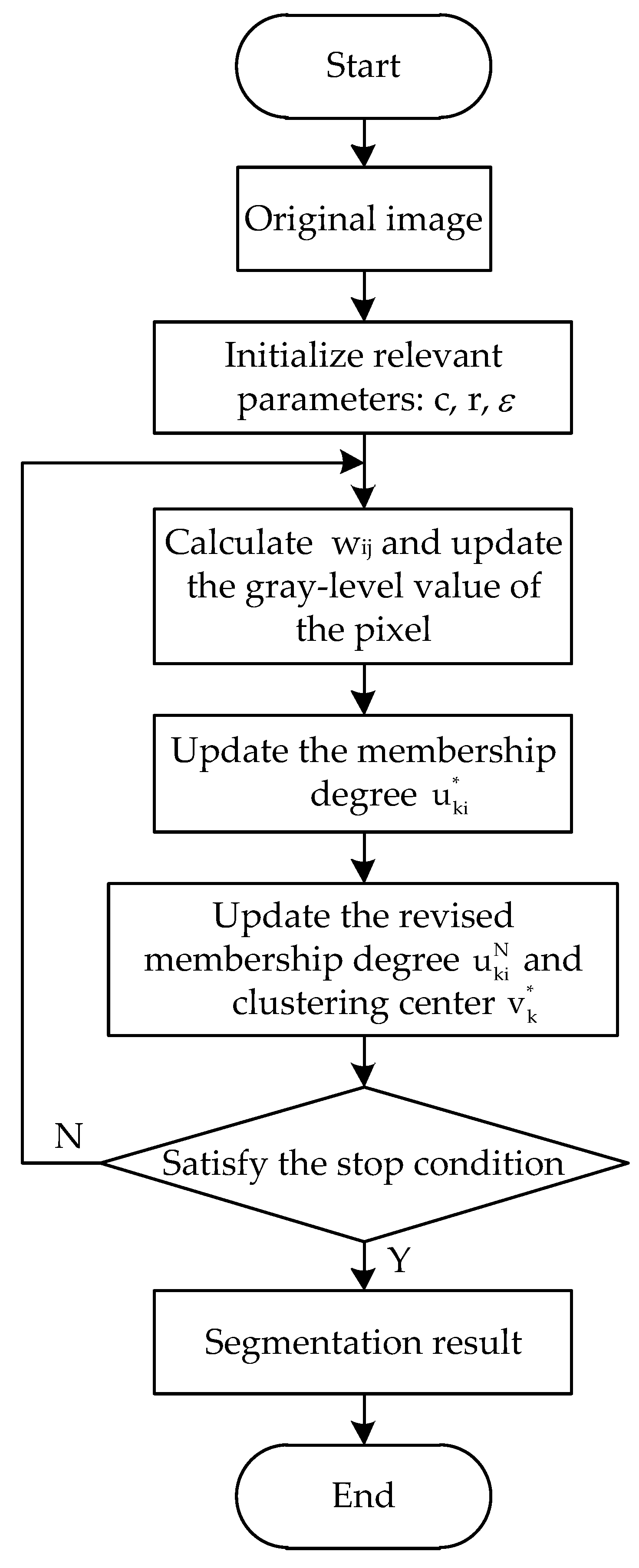
3.4. Program Flowchart

The flowchart for MRFCM is illustrated in Figure 2, and pseudo code of program as follows in Algorithm 1.
Algorithm 1. MRFCM algorithm
Begin
Input:
 original image; % brain MR image to be segmented
 c; % cluster number
 r; % the radius of neighborhood window
 ε; % stop criterion
Initialization: randomly initialize membership degree ukl and cluster center vk and set t = 0
Process:
for t = 0: T iterations
  compute the weighting measure wij using Equation (12) and update gray value ξ i * ;
  compute and update the membership degree u k i * using Equation (14);
  compute and update the revised membership degree u k i N using Equation (16) and clustering
  prototypes v k * using Equation (15);
end
Output: the segmented image
End

4. Experimental Results and Analysis

In order to test and analyze the performance of MRFCM algorithm in this paper, related experiments were carried out on three types of images: synthetic images, simulated brain MR images and real brain MR images. At the same time, five representative image segmentation algorithms were selected to compare with MRFCM: standard FCM, EnFCM [12], FGFCM [13], MICO [19] and ARKFCM [16]. For FCM algorithm and its improved algorithms, the relevant parameters are set as follows: fuzzy exponent m = 2, neighborhood window size of 3 × 3 and stop iteration ε = 0.001. In addition, α = 4 is taken in EnFCM, and λs = 3 and λg = 6 in FGFCM.

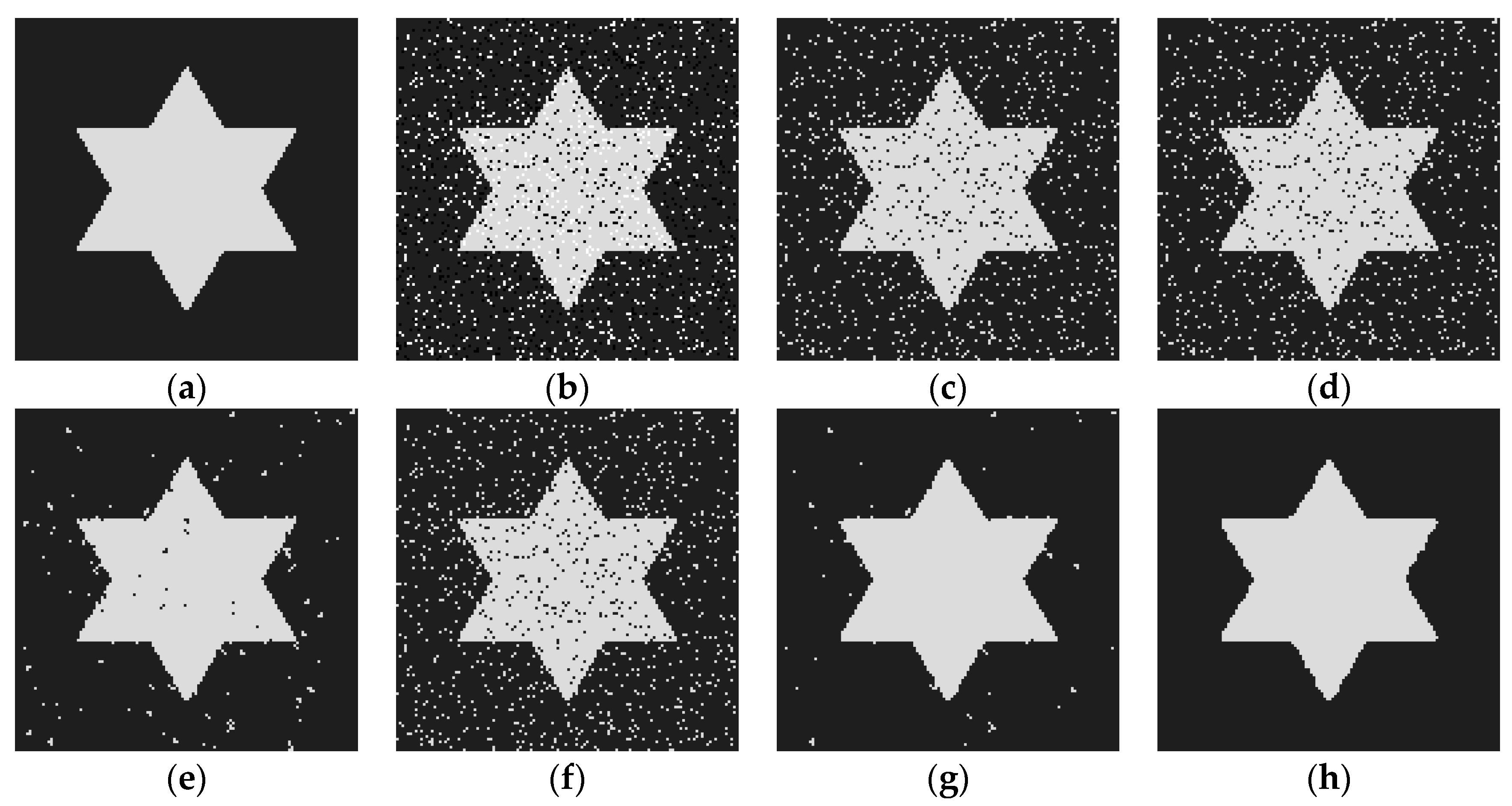
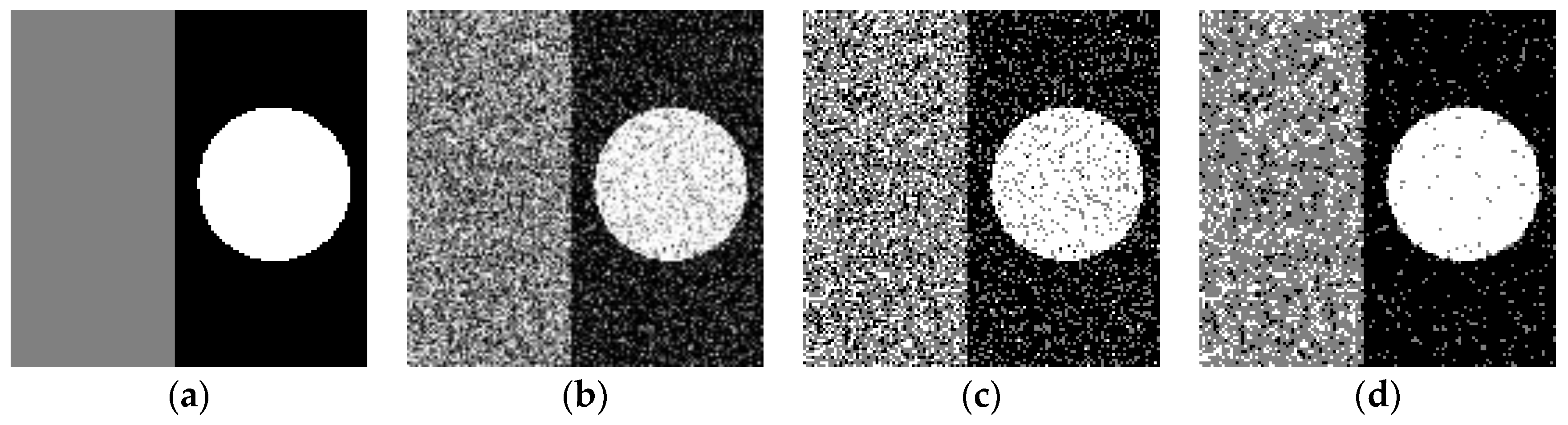
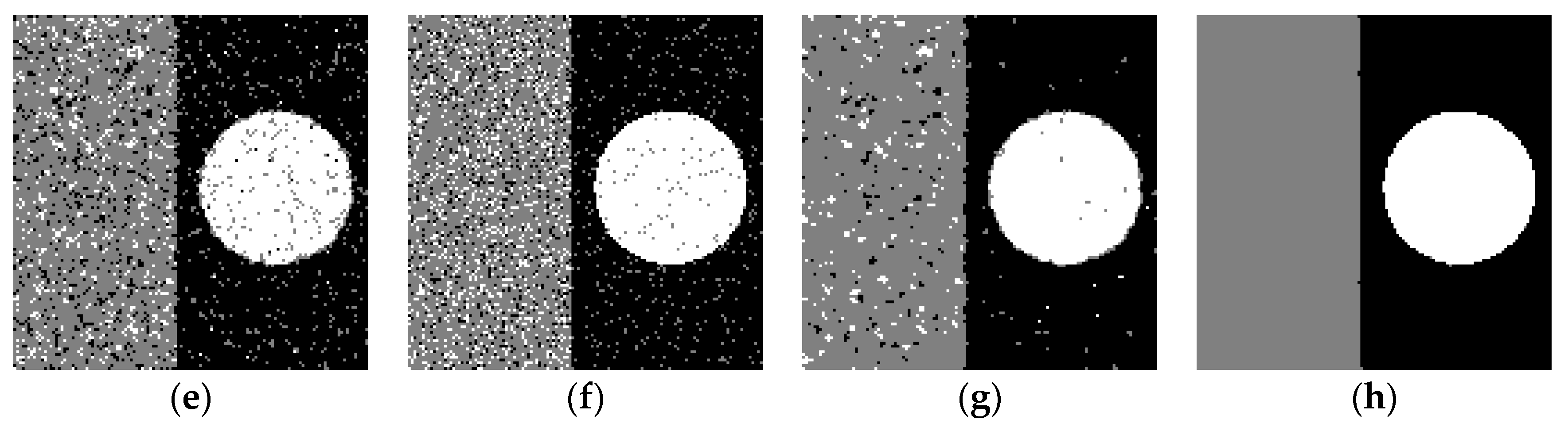
4.1. Synthetic Images

The size of the first synthetic image is 128 × 128 pixels and two pixel gray values: 30 and 220, as shown in Figure 3a. The image was corrupted by 12% salt and pepper noise, as shown in Figure 3b. Six segmentation methods including FCM, EnFCM, FGFCM, MICO, ARKFCM and MRFCM are used to segment the noisy image, and the experimental results are shown in Figure 3c–h. It can be seen from Figure 3 that standard FCM algorithm is very sensitive to pulse-like noise and has almost no noise immunity. Although anti-interference ability is considered in the EnFCM and MICO algorithms, they are almost incapable for salt and pepper noise. FGFCM and ARKFCM algorithms have certain anti-noise ability, but the experimental effect is still not satisfactory. It is obvious that MRFCM has better segmentation result and strong robustness to salt and pepper noise.
The size of the second synthetic image is still 128 × 128 pixels and it contains three gray values: 0, 128 and 255, as shown in Figure 4a. The image is corrupted by zeromean Gaussian noise with standard deviation 0.08, as shown in Figure 4b. Similarly, FCM, EnFCM, FGFCM, MICO, ARKFCM and MRFCM are also used to segment the noisy image, and the experimental results are shown in Figure 4c–h. It can be seen from Figure 4 that the EnFCM algorithm is robust to Gaussian noise, but its effect is not very satisfactory. The rest of the FGFCM, MICO, ARKFCM and MRFCM have the ability to resist Gaussian noise. Obviously, MRFCM has the best segmentation effect.
In order to quantitatively analyze and evaluate the experimental results, Table 1 gives the average segmentation accuracy (SA) of the above six algorithms under different noise level, SA is defined as the ratio of the number of correctly classified pixels to the total number of pixels in the image [20], as follows
S A = i = 1 c A i C i j = 1 c C j
where c is the number of cluster, Ai is the pixel number belonging to the ith cluster found by the algorithm, and Ci is the pixel number belonging to the ith cluster in ground truth. It can be clearly shown from the experimental results in Table 1, MRFCM has higher segmentation accuracy, and it is more robust to noise than the other five algorithms.

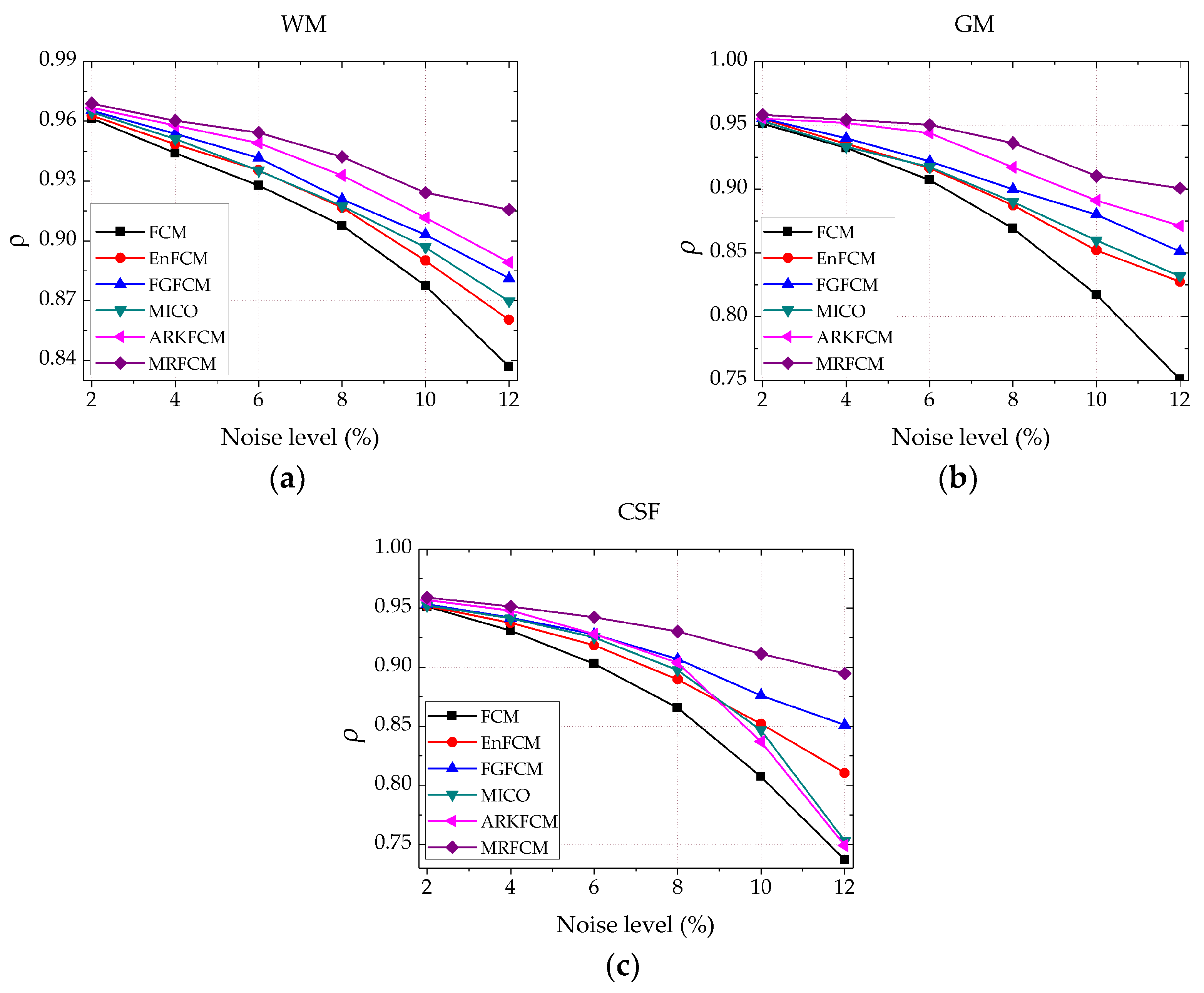
4.2. Simulated Brain MR Images

It is difficult to quantitatively evaluate the performance of segmentation algorithm because the ground truth (GT) of real brain MR image usually does not exist in clinical practice. Brainweb, developed by the brain imaging center of the Montreal Neurology Institute at McGill University, provides a synthetic brain database (SBD) [21], including a set of data generated by an MRI simulator that is close to real brain MR images. The brain MR image data in SBD is composed of a three-dimensional matrix of 181 × 217 × 181 voxels, which can simulate T1, T2 and PD (Proton-density) weighted brain MR images, and the slice thickness, noise level and intensity inhomogeneity can be set by oneself. According to the requirement of the research task, 3D image can be sliced and extracted from three planes (axial, sagittal and coronal) to obtain 2D image data.
In this section, 9 T1 weighted brain MR images are selected as test samples, and 3D brain MR images are sliced from the axial, sagittal and coronal plane, respectively. In Figure 5, The serial numbers are 98, 108 and 96, the slice thickness is 1 mm. and skull, blood vessels and muscle tissue and so on have been removed before the experiment. Noise level in the image is 9%, there is no intensity inhomogeneity, and three slice images are shown in Figure 5a. In general, the structure of brain tissue is very complex, but the brain MR image is generally divided into four parts in clinical applications: white matter (WM), gray matter (GM), cerebrospinal fluid (CSF) and background. In this section, the simulated brain MR images are still tested using six methods: FCM, EnFCM, FGFCM, MICO, ARKFCM and MRFCM. The segmentation results are shown in Figure 5b–g, and GT is illustrated in Figure 5h. It can be seen from the experimental results that the standard FCM without considering spatial information of the neighborhood is very sensitive to noise and cannot accurately segment the noisy MR image. The improved FCM algorithms with local neighborhood constraints, because the spatial neighborhood information are considered in these algorithms, the segmentation validity is improved compared with standard FCM. In these improved methods, EnFCM and MICO algorithms have weak robustness to noise, and the segmentation effect of FGFCM and ARKFCM is relatively good, but they are not ideal for the processing of the edge structure of the brain tissue. By comparing with GT, MRFCM has the best matching degree and the best segmentation results.
As a quantitative evaluation index of segmentation result, the dice coefficient is used to compare the segmentation performance of the six algorithms for simulated brain MR images [22], and the dice coefficient is defined as follows
ρ ( S 1 , S 2 ) = 2 | S 1 S 2 | | S 1 | + | S 2 |
where S1 and S2 represent the segmented image by the evaluated algorithm and GT respectively and | | indicates the number of pixels in the corresponding operation. ρ [ 0 , 1 ] , the larger the value of ρ , the better the segmentation performance. In Figure 6, Dice coefficients of WM, GM and CSF obtained by the above six algorithms are illustrated respectively. As can be seen from the data curve, with the change of noise level, the value of the dice coefficient also changes accordingly. Comparing the magnitude of the ρ value, the strong robustness of the MRFCM is further verified. ARKFCM algorithm has an over-smoothing problem at the edges and details, which leads to the Dice coefficient decreasing sharply and the worse segmentation performance with the increase of noise in CSF extraction. The performance of the MRFCM in this paper is very stable, and it can effectively extract various brain tissues.

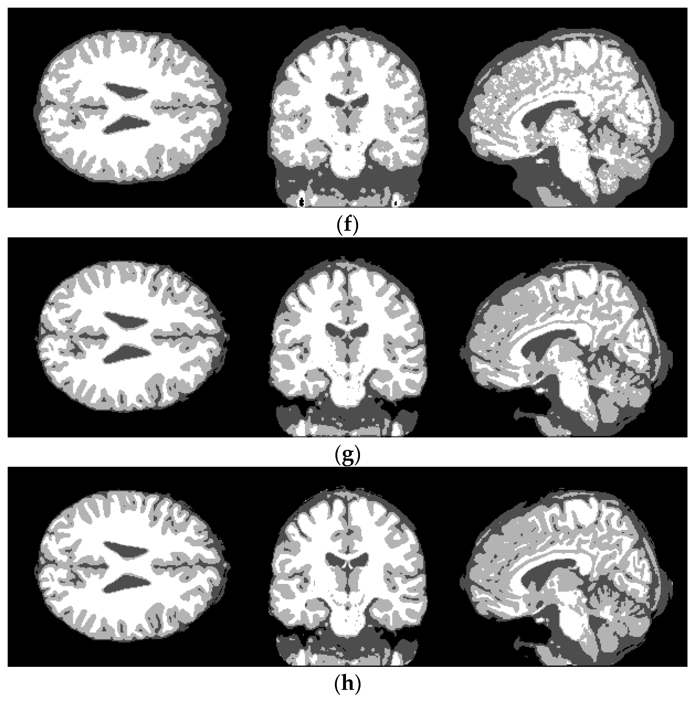
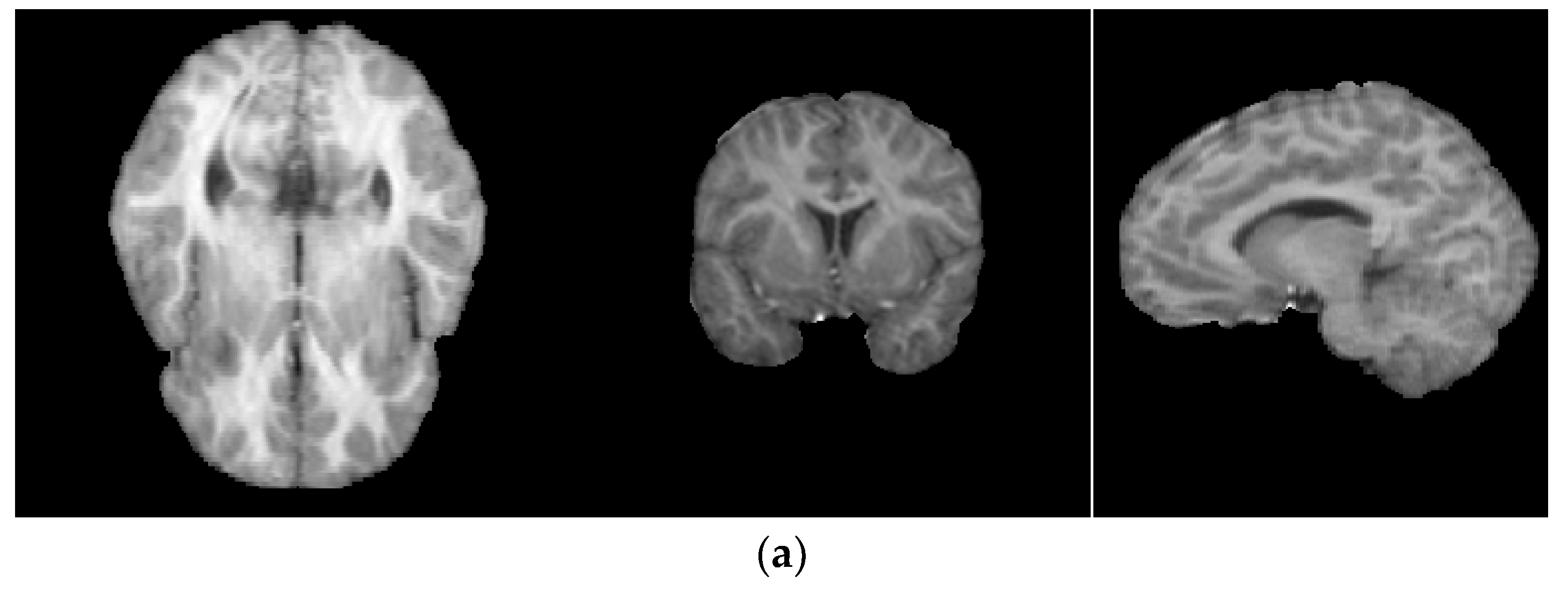
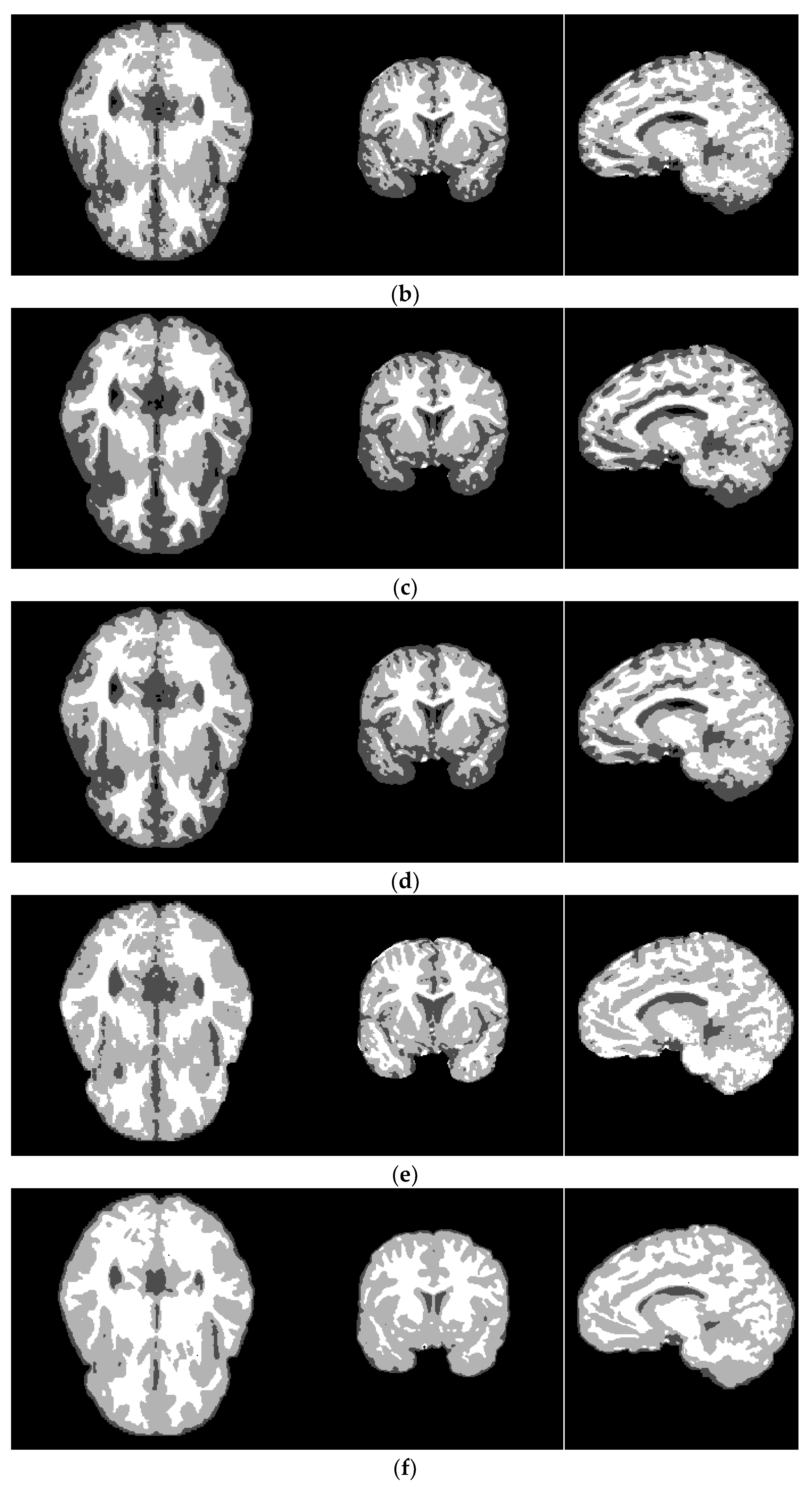
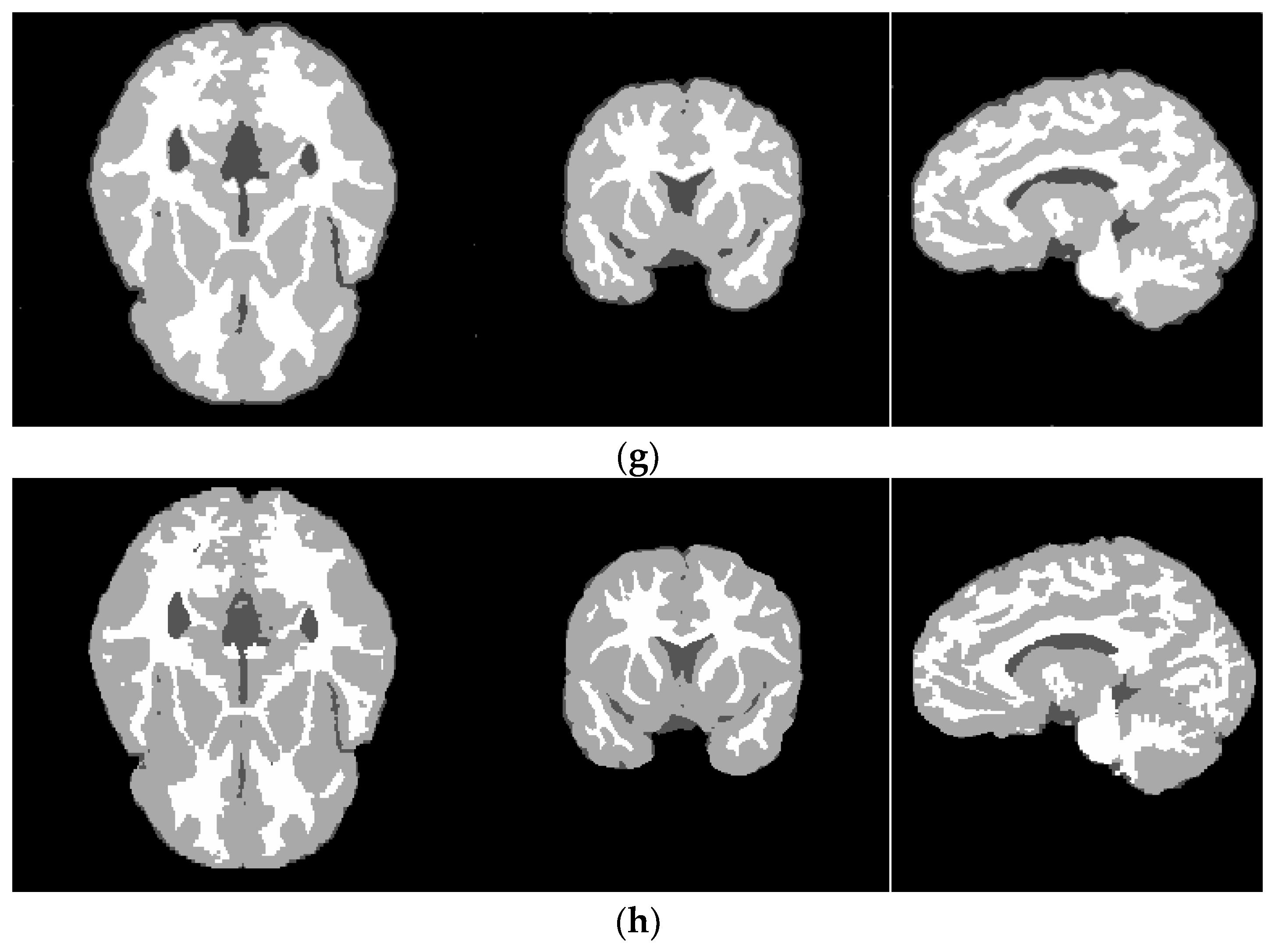
4.3. Real Brain MR Images

In order to more fully verify the performance of the algorithm, an experiment was performed for real brain MR images from Internet Brain Segmentation Repository (IBSR) database provided by Formal Measurement Center (CMA) of Massachusetts General Hospital [23]. IBSR database is a set of clinical data generated by real MRI scans, which contains different levels of noise, and there are also varying degrees of intensity inhomogeneity, covering various problems that may arise in real MR data segmentation.
In experiments, we still selected 9 T1-weighted real brain MR images from IBSR database. In Figure 7, three sliced images are extracted from 3D brain MR data from axial, sagittal, and coronal plane, respectively. The corresponding numbers are 127, 76 and 116, as shown in Figure 7a, and the ground truth images of these images are also given, as shown in Figure 7h. Segmentation algorithms still adopt FCM, EnFCM, FGFCM, MICO, ARKFCM and MRFCM, and the segmentation results are shown in Figure 7b–g. It can be clearly seen that the segmentation result of the MRFCM is closest to ground truth, which further validates the effectiveness of the algorithm in real brain MR images.

4.4. Selection of Window Radius r

For the same brain MR image is corrupted by different noise-level, the segmentation accuracy of each radius r is shown in Table 2.
As can be seen from Table 2, with the noise increasing, the segmentation accuracy gradually decreases. When variance σ ≤ 0.35, the window radius r = 1 corresponds to the highest segmentation accuracy. The increase of the window radius leads to a decrease in segmentation accuracy because the large window can well overcome the influence of noise, but it is easy to erase the details and edge parts of the image, so the segmentation accuracy is reduced. When σ > 0.35, the segmentation accuracy corresponding to the window radius r = 1 will drop significantly, and the segmentation effect is poor. The segmentation accuracy is the highest when the window radius r = 3. It can be seen that the larger the window radius, the stronger the anti-noise ability of MRFCM, but the segmentation accuracy is worse. On the other hand, the larger the window radius is, the higher the computational complexity of the algorithm. Based on the consideration of segmentation accuracy and computational complexity for brain MR images, when the noise level is small, the image can be segmented with the window radius r = 1, and when the image noise level is larger, the window radius r = 3 is used.

5. Conclusions

In the process of brain magnetic resonance imaging, noise interference is an inherent defect. In medical image segmentation, it will affect the segmentation accuracy of brain tissue extraction, and may further affect the treatment effect in clinical diagnosis. A modified FCM scheme incorporating spatial neighborhood information is proposed in this paper, which has strong anti-noise ability, and the algorithm is simple and the calculation speed is fast. MRFCM is applied to three types of images: synthetic images, simulated brain MR images and real brain MR images, and compared the experimental results with standard FCM and several state-of-the-art improvement schemes based on FCM. The experimental results show that MRFCM is robust to noise and can accurately segment noisy brain MR images. Our future work will focus on reducing its computational complexity by incorporating convex optimization techniques, the extension of the existing algorithm to 3D data and multi-modal image segmentation.

Author Contributions

Conceptualization, J.S.; methodology, J.S. and Z.Z.; software, Z.Z.; formal analysis, J.S.; data curation, Z.Z.; writing—original draft preparation, J.S. and Z.Z.; writing—review and editing, J.S.; supervision, J.S.; funding acquisition, J.S.

Funding

This work is partially supported by Principal Fund Project of Minnan Normal University (Grant No. KJ18010) and the Education and Teaching Reform Project of Undergraduate Colleges and Universities in Fujian Province (Grant No. FBJG20180015).

Conflicts of Interest

The authors declare no conflict of interest.

References

  1. Balafar, M.A.; Ramli, A.R.; Saripan, M.I.; Mashohor, S. Review of brain MRI image segmentation methods. Artif. Intell. Rev. 2010, 33, 261–274. [Google Scholar] [CrossRef]
  2. Khorram, B.; Yazdi, M. A New Optimized Thresholding Method Using Ant Colony Algorithm for MR Brain Image Segmentation. J. Digit. Imaging 2018, 1–13. [Google Scholar] [CrossRef] [PubMed]
  3. Meng, X.; Gu, W.; Chen, Y.; Zhang, J. Brain MR image segmentation based on an improved active contour model. PLoS ONE 2017, 128, e0183943. [Google Scholar] [CrossRef] [PubMed]
  4. Pereira, S.; Pinto, A.; Oliveira, J.; Mendrik, A.M.; Correia, J.H.; Silva, C.A. Automatic brain tissue segmentation in MR images using Random Forests and Conditional Random Fields. J. Neurosci. Methods 2016, 270, 111–123. [Google Scholar] [CrossRef] [PubMed]
  5. Moeskops, P.; Viergever, M.A.; Mendrik, A.M.; de Vries, L.S.; Benders, M.J.; Išgum, I. Automatic segmentation of MR brain images with a convolutional neural network. IEEE Trans. Med. Imaging 2016, 35, 1252–1261. [Google Scholar] [CrossRef] [PubMed]
  6. Rajaby, E.; Ahadi, S.M.; Aghaeinia, H. Robust color image segmentation using fuzzy c-means with weighted hue and intensity. Digit. Signal Process. 2016, 51, 170–183. [Google Scholar] [CrossRef]
  7. Saha, S.; Alok, A.K.; Ekbal, A. Brain image segmentation using semi-supervised clustering. Expert Syst. Appl. 2016, 52, 50–63. [Google Scholar] [CrossRef]
  8. Namburu, A.; Kumar, S.S.; Edara, S.R. Generalized rough intuitionistic fuzzy c-means for MR brain image segmentation. IET Image Process. 2017, 11, 777–785. [Google Scholar] [CrossRef]
  9. Chetih, N.; Messali, Z.; Serir, A.; Ramou, N. Robust fuzzy c-means clustering algorithm using non-parametric Bayesian estimation in wavelet transform domain for noisy MR brain image segmentation. IET Image Process. 2018, 12, 652–660. [Google Scholar] [CrossRef]
  10. Bezdek James, C. Pattern Recognition with Fuzzy Objective Function Algorithms. Adv. Appl. Pattern Recognit. 1981, 22, 203–239. [Google Scholar]
  11. Pedrycz, W.; Waletzky, J. Fuzzy clustering with partial supervision. IEEE Trans. Syst. Man Cybern. B 1997, 27, 787–795. [Google Scholar] [CrossRef] [PubMed]
  12. Szilagyi, L.; Benyo, Z.; Szilagyi, S.M.; Adam, H.S. MR brain image segmentation using an enhanced fuzzy C-means algorithm. In Proceedings of the Annual International Conference on Engineering in Medicine & Biology Society, Cancun, Mexico, 17–21 September 2003; pp. 724–726. [Google Scholar]
  13. Cai, W.; Chen, S.; Zhang, D. Fast and robust fuzzy c-means clustering algorithms incorporating local information for image segmentation. Pattern Recognit. 2007, 40, 825–838. [Google Scholar] [CrossRef]
  14. Despotovic, I.; Vansteenkiste, E.; Philips, W. Spatially Coherent Fuzzy Clustering for Accurate and Noise-Robust Image Segmentation. IEEE Signal Process. Lett. 2013, 20, 295–298. [Google Scholar] [CrossRef]
  15. Ji, Z.; Liu, J.; Cao, G.; Sun, Q.; Chen, Q. Robust spatially constrained fuzzy c-means algorithm for brain MR image segmentation. Pattern Recognit. 2014, 47, 2454–2466. [Google Scholar] [CrossRef]
  16. Elazab, A.; Wang, C.; Jia, F.; Wu, J.; Li, G.; Hu, Q. Segmentation of Brain Tissues from Magnetic Resonance Images Using Adaptively Regularized Kernel-Based Fuzzy C-Means Clustering. Comput. Math. Methods Med. 2015, 485495. [Google Scholar]
  17. Ahmed, M.N.; Yamany, S.M.; Mohamed, N.; Farag, A.A.; Moriarty, T. A modified fuzzy c-means algorithm for bias field estimation and segmentation of MRI data. IEEE Trans. Med. Imaging 2002, 21, 193–199. [Google Scholar] [CrossRef] [PubMed]
  18. Chuang, K.S.; Tzeng, H.L.; Chen, S.; Wu, J.; Chen, T.J. Fuzzy c-means clustering with spatial information for image segmentation. Comput. Med. Imag. Graphics 2006, 30, 9–15. [Google Scholar] [CrossRef] [PubMed]
  19. Li, C.; Gore, J.C.; Davatzikos, C. Multiplicative intrinsic component optimization (MICO) for MRI bias field estimation and tissue segmentation. Magn. Reson. Imaging 2014, 32, 913–923. [Google Scholar] [CrossRef] [PubMed]
  20. Li, C.; Huang, R.; Ding, Z.; Gatenby, J.C.; Metaxas, D.N.; Gore, J.C. A Level Set Method for Image Segmentation in the Presence of Intensity Inhomogeneities With Application to MRI. IEEE Trans. Image Process. 2011, 20, 2007–2016. [Google Scholar] [PubMed]
  21. BrainWeb, Simulated Brain Database. Available online: http://brainweb.bic.mni.mcgill.ca/brainweb/ (accessed on 17 August 2004).
  22. Vovk, U.; Pernus, F.; Likar, B. A Review of Methods for Correction of Intensity Inhomogeneity in MRI. IEEE Trans. Med. Imaging 2007, 26, 405–421. [Google Scholar] [CrossRef] [PubMed]
  23. The Internet Brain Segmentation Repository (IBSR). Available online: http://www.nitrc.org/projects/ibsr (accessed on 4 January 2016).
Figure 1. The normalized weight coefficient of each pixel in the neighborhood.
Information 10 00074 g001
Figure 2. Flowchart of the proposed algorithm.
Information 10 00074 g002
Figure 3. The segmentation results of salt & pepper noise-corrupted synthetic image. (a)original image; (b) noisy image; (c) FCM result; (d) EnFCM result; (e) FGFCM result; (f) MICO result; (g) ARKFCM result; (h) MRFCM result.
Information 10 00074 g003
Figure 4. The segmentation results of Gaussian noise-corrupted synthetic image. (a) original image; (b)noisy image; (c) FCM result; (d) EnFCM result; (e) FGFCM result; (f) MICO result; (g) ARKFCM result; (h) MRFCM result.
Information 10 00074 g004aInformation 10 00074 g004b
Figure 5. The segmentation results of simulated brain MR images by six algorithms. (a) noisy brain MR images; (b) segmentation results of FCM; (c) segmentation results of EnFCM; (d) segmentation results of FGFCM; (e) segmentation results of MICO; (f) segmentation results of ARKFCM; (g) segmentation results of MRFCM; (h) ground truth
Information 10 00074 g005aInformation 10 00074 g005b
Figure 6. Dice coefficient comparison of MR image segmentation results under different noise level. (a) the curve of the dice coefficient about WM; (b) the curve of dice coefficient about GM; (c) the curve of the dice coefficient about CSF.
Information 10 00074 g006
Figure 7. The segmentation results of three real brain MR images with different algorithms. (a) brain MR images; (b) segmentation results of FCM; (c) segmentation results of EnFCM; (d) segmentation results of FGFCM; (e) segmentation results of MICO; (f) segmentation results of ARKFCM; (g) segmentation results of MRFCM; (h) ground truth.
Information 10 00074 g007aInformation 10 00074 g007bInformation 10 00074 g007c
Table 1. The comparison of SA values under different noise level.
Noise TypeNoise Level (%)FCMEnFCMFGFCMMICOARKFCMMRFCM
Salt and pepper noise40.98030.98810.99440.98760.99880.9995
80.95760.96220.99020.95990.99700.9991
120.93850.94360.98750.94350.99430.9976
160.92030.92910.96850.92130.98720.9923
Gaussian noise40.81540.95990.96110.95070.97980.9993
80.69210.85090.87680.86100.95400.9985
120.63460.78250.82690.79670.94530.9912
160.60160.71410.78770.72330.93140.9872
Table 2. Comparison of segmentation accuracy between different noise level and different.
Noise VarianceRadius r
12345
0.050.99620.99490.98810.98640.9816
0.150.99350.99150.98340.97580.9701
0.250.98930.98660.98220.97070.9615
0.350.98470.97420.96180.95890.9523
0.650.80190.84310.90070.86520.8712
0.950.61280.67930.73860.74360.7528

