Article

Routing Algorithm Based on Trajectory Prediction in Opportunistic Networks

School of Software, Railway College, Central South University, Changsha 410075, China
*
Author to whom correspondence should be addressed.
Information 2019, 10(2), 49; https://doi.org/10.3390/info10020049
Submission received: 17 January 2019 / Revised: 28 January 2019 / Accepted: 29 January 2019 / Published: 4 February 2019
(This article belongs to the Section Information Applications)

Abstract

:
Due to the dynamic change of the opportunistic network topology and the lack of stable information transmission paths between nodes, the traditional topology-based routing algorithm cannot achieve the desired routing performance. To address of this problem, this paper proposes a routing algorithm based on trajectory prediction (RATP). The routing protocol based on trajectory prediction can efficiently and quickly adapt to the network link quality instability and the dynamic changes of network topology. RATP algorithm constructs a node mobility model by analyzing the historical mobility characteristics of the nodes. According to the node prediction information, the metric value of the candidate node is calculated, and the node with the smaller metric value is selected as the data forwarding node, which can effectively reduce the packet loss rate and avoids excessive consumption. Simulation results show that compared with other algorithms, the proposed algorithm has higher data delivery ratio, and end-to-end data delay and routing overhead are significantly reduced.

1. Introduction

An opportunistic network is a kind of network that can construct communication services between nodes with the network structure fracture and topology dynamic change. It has extensive research and application value in military and civilian fields [1,2].
At present, the main research hotspots of the opportunistic networks are: routing algorithms, network information security [3], energy research, mobility model research and so on. The topology of the opportunistic networks changes dynamically and no relatively stable data transmission path between nodes. This makes it difficult to achieve more efficient performance based on the change of network topology [4]. Therefore, how to find a routing protocol with good routing performance is one of the most challenging problems in opportunistic networks research. Opportunistic network routing protocols face the following challenges:
  • Unevenness of opportunities to encounter between nodes. In the opportunistic network, the information interaction occurs only when two nodes enter each other’s communication range. The chance of encountering between the two nodes is unpredictable, which leads to the imbalance of the chances of encountering the nodes.
  • Topology structure information is difficult to grasp. The topology of the opportunistic network changes dynamically, and the mobile information of nodes in the network is difficult to obtain accurately and timely.
  • Resource constraints. Most of the opportunistic network nodes are portable devices, so the nodes themselves have limitations such as energy, contact time, and storage space.
  • Unpredictability of node movement trajectory. The mobile behavior of a node is affected by many external factors, and it is impossible to obtain the precise location information of the node in time.
At present, researchers have proposed many opportunistic network routing protocols. The opportunistic network information transmission mechanism is “store-carry-forward”. According to the routing strategy, it can be divided into three categories: code-based, scene-based and switched-based routing [5]. However, they did not consider the location information of the node. The location information of the node plays an important role in quickly discovering the information of the next-hop forwarding node. At present, there are some location-based routing algorithms [6,7]. In these algorithms, the next-hop forwarding node can be found through the location information of the neighbor and destination nodes, which effectively improves the routing performance and has strong adaptability to the dynamic change of the network topology. The DIG (Direction based geographic routing scheme) [8] algorithm is a representative location-based algorithm. However, the algorithm does not fully utilize the location information of the neighbor nodes, which makes the delay performance unsatisfactory and requires improvement. The LAR (Location Aided Routing) [9] algorithm and the LOTAR (Location Trace Aided Routing) algorithm [10] establish a source node to a destination node route by directly utilizing location information, thereby transmitting data packets. GPSR (Greedy Perimeter Stateless Routing) [11] algorithm and GLS (Grid Location Service) [12] algorithm also transmit information by using node location information, but the two algorithms do not establish a data transmission path from the source node to the destination node.
To solve the problems, this paper proposes a routing algorithm based on trajectory prediction. This approach is based on the historical mobility characteristics of the nodes to establish the mobility model of the node. Based on the predicted location information, the metric value of the candidate node is calculated, and the node with the smaller metric value is selected as the data forwarding node. The presented method may be successfully used for vehicular ad hoc networks (VANETs).
The main contributions of this article are in the following areas:
(1)
Constructing the node mobility model based on the historical mobility characteristics of the node. By changing the value of the node’s mobile coordination factor, the possible running speed of the node at the next moment is obtained.
(2)
Using the Gaussian process to model the speed probability of different mobile coordination factors, and using the maximum likelihood estimation (EM) algorithm to obtain the model parameters, so that the probability of speed based on historical mobility characteristics is best. On this basis, the node movement distance and node location information are calculated.
(3)
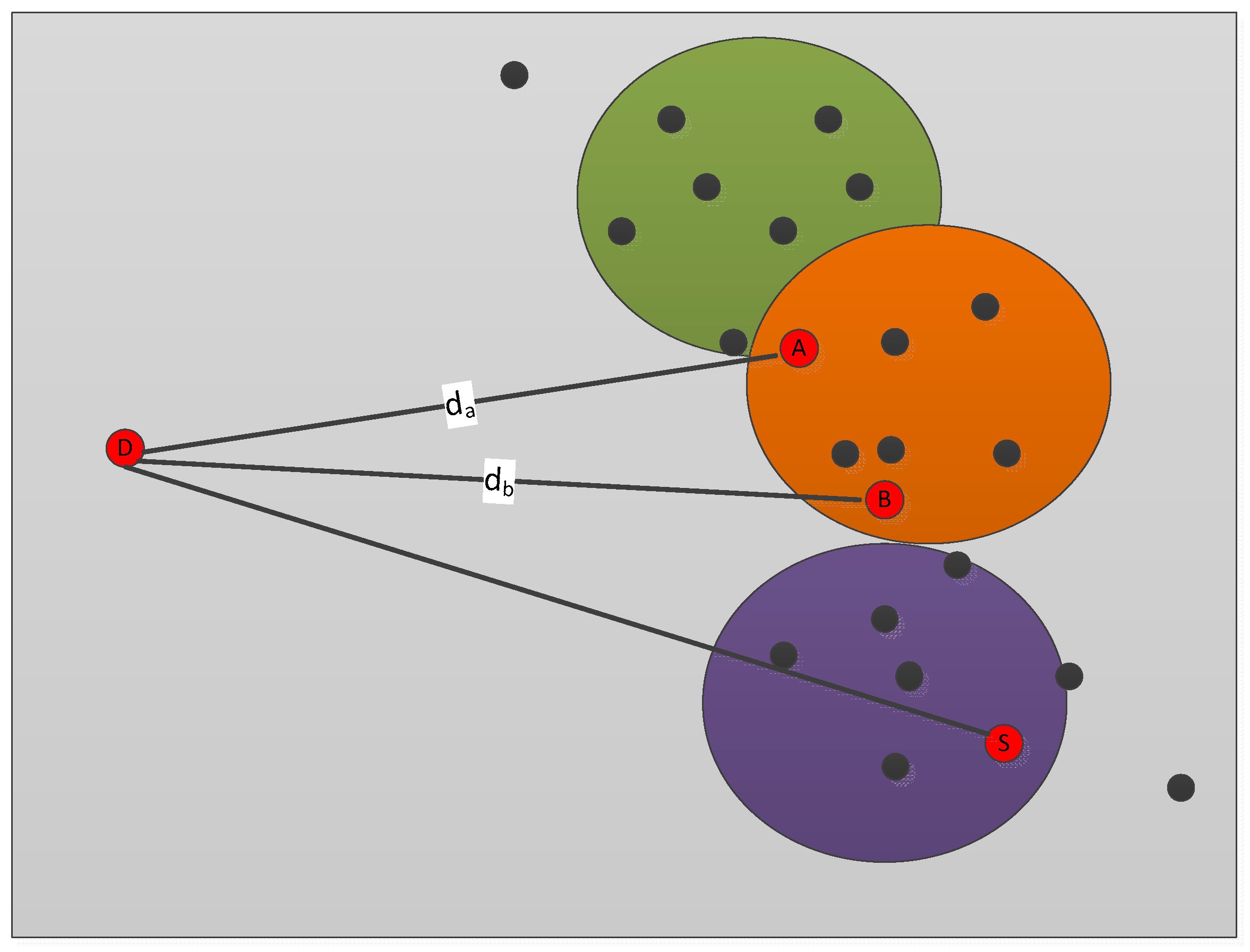
Calculating the metric value of the candidate node based on the predicted location information. During the information transmission, the node does not need to store too much routing information, and the network resource consumption is significantly reduced. The use of the location information can effectively avoid loop generation during data delivery and also have strong adaptability to the dynamic network topology change.
(4)
The simulation platform ONE simulates a large amount of data and evaluates the performance of the RATP algorithm, with improved transmission success rate, reduced data delay and routing overhead.
The rest of this paper mainly includes the following parts: the second part analyzes some existing research works; the third part analyzes and describes the algorithm; simulation results are presented in Section 4. The last section concludes this paper.

2. Related Work

Many previous research results have shown that the acquisition of node location information has a very significant impact on the performance of the opportunistic network routing. At present, the way to obtain location information of nodes is mainly through location system. When a node transmits information, it only needs to obtain the location information of the neighbor and destination node to select the appropriate next-hop node, thus reducing the network resource overhead. Nodes only need to obtain location information, which can improve the utilization of network bandwidth. The distance between neighbors can be calculated by using location information, which can save energy consumption [13].
In recent years, the routing algorithm based on location information has many advantages over the routing algorithm based on network topology, so the routing protocol based on location information has attracted the attention of many researchers [14,15,16]. According to the routing strategies, location-based routing can be roughly divided into two categories: proactive routing protocol and reactive routing protocol. Among them, proactive routing protocols represent algorithms such as LOTAR, GPSR, DREAM, and reactive routing protocols represent algorithms such as LAR, GLS, DIG, etc. LAR routing protocol is a location aided routing algorithm. Based on the node location information, the algorithm finds the path of data transmission so as to narrow the routing search area and improve the data delivery ratio. In the LAR [9] algorithm, each node carries a positioning system that can obtain its current location information at any time, and assumes that each node in the network knows the mobility rate of other nodes. GLS [12] is a hierarchical routing protocol consisting of two parts: location information acquisition and data forwarding. The GLS algorithm divides the whole network into several small grids. The nodes in the grid periodically broadcast their own geographical location information. The other nodes update their own location information table according to the broadcast information. The nodes outside the grid act as the location information server through the selected nodes in the grid. By using these nodes to update and query the location information in time, the neighbor nodes closest to the destination node are selected as the next-hop data forwarding node. DREMA (Distance routing effect algorithm for mobility) [17] algorithm shows that each node in the network carries its own location information and periodically broadcasts the information. Other nodes in the network receive the location information, update and store the new location information in their own location information table. This method can effectively reduce the network control information overhead and ensure the accuracy of the link information. Although the algorithm has very good performance, it is not suitable for networks with relatively large network topology, and the performance of the algorithm will gradually decrease when the path between nodes does not exist.
The approach in [18] proposes a Centrality History-Based Prediction Routing Protocol (CHBPR). The algorithm focuses on the use of the concept of centrality to achieve information transfer between nodes. Unlike other nodes in the network, the central node is more likely to act as a communication hub for message forwarding. Dhurandher et al. [19] proposed a centrally-based mechanism (HiBOp) to improve the performance of history-based routing protocols. GEAR [20] is an algorithm of greedy forwarding and energy efficiency. The core idea of the GEAR is to combine the energy information of each neighbor node with the distance between the neighbor node and the destination node when selecting the next-hop data forwarding node. GR (Greedy Routing) [21], the selection of the next-hop forwarding node must satisfy that the node is the closest distance to the target node among all neighbor nodes, and the distance is smaller than the distance from the current node to the target node. By searching the network, the node satisfying the condition is found as the optimal next-hop data forwarding node for data delivery.
Reference [22] proposed a new method to find the nearest neighbor from the current sending node in a given angle range as the next-hop node. In the routing algorithm based on location information, the greedy data forwarding strategy is the most efficient and simple. Based on the definition of the particle fitness function with neighbor node information, a single-hop routing clustering protocol (DPSOCA) based on discrete particle swarm optimization is proposed in [23]. Reference [24] proposed a new routing protocol called greedy peripheral coordinator routing (GPCR) algorithm, which does not require external information of the node, nor the entire network information. It only realizes the data forwarding between nodes by coordinating the relationship between nodes. However, it is easy for this selection mechanism to fail in the case of low node density. The improved greedy traffic sensing routing protocol [25] is mainly characterized by considering node density before forwarding data packets.

3. RATP

Each node carries its own location information (LM) and neighbor node information table (NT), and broadcasts the information at a certain interval. Where the LM information is expressed as follows: LM (Location, velocity) indicates location information, which refers to a message that carries location information and can be broadcast within a certain range. Location: it is indicated by the two-dimensional coordinates of node (xi, yi), while the velocity is specified by the current moving speed value of the node and the direction of node movement.

3.1. Trajectory Prediction

3.1.1. Node Mobility Model

In this paper, through the LM information carried by the node itself, the mobility characteristics of the node are analyzed, and the appropriate node mobility model is constructed. The average node moving speed in a long period of time is calculated by analyzing the node moving speed.
J = lim t ( t = 0 v i t )
We assume that the node mobility satisfies the Gaussian distribution. According to the historical movement information of the node, the motion state of the node in the future motion state is analyzed. Use δ n to indicate the state of the node moving in the future.
δ n = 1 λ × 2 π e n 2 2 λ 2
In the above formula, λ is the node mobile coordination factor, satisfies 0 λ 1 . The magnitude of λ represents the mutation of node speed in a short time, and it is a specific performance of the node itself mobility performance. Therefore, the node mobility model can be defined as follow:
v t + Δ t = ( ( λ 1 ) v t + ( 1 λ ) J + 1 λ 2 δ n ) Δ t
At t + Δ t moment, the value of the node’s moving speed v t + Δ t is obtained by the influence of the average node moving speed in a long period of time, the random state of the node moving in the future and the moving coordination factor on the speed.
However, a simple next-time velocity value does not produce a relatively high and stable prediction accuracy for node trajectory prediction, and different mobile coordination factor values will have a corresponding impact on the next-time moving speed value.

3.1.2. Probability of Node Velocity

Suppose that each data point v i can be obtained by transformation the data point λ i through Λ λ j + μ ( Λ is a matrix) deformation. Because the historical track GPS data often have noise, we can assume that the noise data also obeys the Gauss distribution, that is χ N ( 0 , ψ ) , so the predicted data is μ + Λ λ + χ . The trajectory probability model can be obtained as follows:
p ( V | λ ) = j = 1 k j = 1 k σ j φ ( v j | μ j + Λ λ j , ψ j )
where σ j is the weight of the j Gaussian process and satisfy σ j 0 , j = 1 k σ j = 1 , φ ( ) represents the Gauss process probability density function, and k represents the number of Gauss processes. Using the Gauss hybrid model to estimate the parameter σ ,   μ ,   Λ ,   ψ accurately. In general, the expectation-maximization algorithm is used to estimate the parameters of the GMM model. A set of parameters was found through iterative training to maximize the value of p ( V | λ ) , that is:
( σ ,   μ ,   Λ ,   ψ ) = arg max ( σ ,   μ ,   Λ ,   ψ ) p ( V | λ )
Because each xi is transformed by the corresponding λ j , plus the noise, so V is the posterior distributions of λ : V | λ N ( μ v + Λ λ v , ψ v ) . Therefore, λ and V obey the joint Gaussian distribution:
[ v λ ] N ( μ v λ , Σ )
Due to the fact that λ follows a normal distribution with a mean of zero, therefore E ( λ ) = 0 . All elements of the matrix Λ are constants, and their expected value is still itself, so you can get μ v λ = [ 0 μ ] .
Solving   Σ requires calculation
Σ λ λ = E [ ( λ E [ λ ] ) ( λ E [ λ ] T ) ]
Σ v λ = E [ ( λ E [ λ ] ) ( v E [ v ] T ) ]
Σ v v = E [ ( v E [ v ] ) ( v E [ v ] T ) ]
Σ λ λ = C o v ( λ ) = 1 , E [ ( λ E [ λ ] ) ( v E [ v ] T ) ] = Λ T . And E [ ( v E [ v ] ) ( v E [ v ] T ) ] = Λ Λ T + ψ can be obtained from the E [ λ λ T ] = C o v ( λ ) , E [ λ χ T ] = E [ λ ] E [ χ T ] = 0 . So the edge distribution of V is as follows: v N ( μ ,   Λ Λ T + ψ ) and the conditional distribution v N ( μ + ( Λ Λ T + ψ ) Λ T 1 λ j ,   Λ ( Λ Λ T + ψ ) Λ T 1 1 ) . Set of training trajectories data sets { v j ; j = 1 , 2 , , k } , the logarithmic likelihood function of the parameter ,   Λ ,   ψ is established.
l ( μ , Λ , ψ ) = log j = 1 k 1 ( 2 π ) k / 2 | Λ Λ T + ψ | 1 / 2 exp ( 1 2 ( v j μ ) T ( Λ Λ T + ψ ) 1 ( v j μ ) )
The following requires the probability of a further motion pattern i, which requires calculation of the parameter σ and the value obtained when the partial derivative of the parameter μ , Λ , ψ in Equation (10) is zero. Use EM algorithm solution, divided into two steps E-step (seeking expectations) and M-step (seeking extreme value), the specific method is as follows:
Step E: The probability that the node mobile coordination factor is λ j and the node speed is vi.
p ( j | v j , λ ) = σ j p ( v j | j , λ ) p ( v j | λ ) = σ j φ ( v j | μ j + Λ λ j , ψ j ) j = 1 k σ j φ ( v j | μ j + Λ λ j , ψ j )
M-step: using the maximum expectation method to obtain the parameter σ iterative estimation formula:
σ = j = 1 k p ( j | v j , λ )
Maximizing the likelihood function of the parameter μ , Λ , ψ , find the iterative estimation formula of the parameter μ ,   Λ ,   ψ :
j = 1 k λ j log p ( v j , λ j ; μ , Λ , ψ ) λ j d λ j = j = 1 k E [ log p ( v j | λ j ; μ , Λ , ψ ) + log p ( λ j ) log p ( λ j ) ]
Therefore, it can be obtained:
μ = 1 k j = 1 k v j ,    Λ = ( j = 1 k ( v j μ ) μ v j | λ j T ) ( j = 1 k μ v j | λ j μ v j | λ j T + Σ v j | λ j ) 1 ψ = 1 k j = 1 k v j v j T v j μ x j | λ j T Λ T Λ μ v j | λ j T x i T + Λ ( μ v j | λ j μ v j | λ j T + Σ v j | λ j ) Λ T
The μ v j | λ j and Σ x i | z i can be obtained μ v j | λ j = μ + ( Λ Λ T + ψ ) Λ T 1 λ j , Σ v j | λ j = Λ ( Λ Λ T + ψ ) Λ T 1 1 . E-step estimates the weights of the Gauss model by conjecture the parameters of the Gauss model. M-step is the weight of the Gauss model based on the E-step estimate. Repeat the above two steps until the fluctuation is small and approximately reaches the extreme value.

3.1.3. Node Location

The coordinate of node location can be obtained by the node coordinate location at t moment (through LM information) and node moving velocity vector angle.
The location of the node at time t can be identified by coordinates L t ( x t , y t ) , so at time t + Δ t , the geographic location of the node can be predicted based on the speed v t , node position L t ( x t , y t ) , direction β t (speed vector change angle) and speed v t + Δ t at time t.
If in Δ t time, the node driving direction has changed:
( x t + Δ t , y t + Δ t ) = { x t + Δ t = x t + ( v t + Δ t + v t 2 ) Δ t cos β t y t + Δ t = y t + ( v t + Δ t + v t 2 ) Δ t sins β t
If in Δ t time, the node driving direction has not changed:
( x t + Δ t , y t + Δ t ) = { x t + Δ t = x t + ( v t + Δ t + v t 2 ) Δ t y t + Δ t = y t + ( v t + Δ t + v t 2 ) Δ t

3.1.4. Node Moving Distance

The moving distance of the node means the length of the node moves from moment t to moment t + Δ t , which can be denoted by Δ D s . Since the movement of the node in a short period of time approximates a uniform motion, so the distance can be expressed by the displacement formula of the physics:
Δ D s = D s t + Δ t D s t = ( v t + Δ t + v t 2 ) × Δ t
where D s t represents the total moving distance of node in t time. The D s t + Δ t represents the total moving distance of node in t + Δ t time.
D s t + Δ t = D s t + 1 4 × [ θ ( v t + Δ t + v t ) + ( 1 θ ) ( η t + Δ t + η t ) + 1 θ 2 ( ζ t + Δ t + ζ t ) ] Δ t 2

3.2. Data Forwarding Mode

From Section 3.1, the predicted location is obtained. As shown in Figure 1, Node A is the current node and Node D is the destination node. The distance from Node B to line AD is as follows:
d B A D = | ( D 2 x 2 ) B 1 + ( x 1 D 1 ) B 2 + ( d 1 x 1 ) ( x 2 x 1 ) | d 0
The formula of the relative deflection angle is:
α = arcsin d B A D d ,   α [ 0 , π 4 ]
Calculating the metric value of the candidate node based on the predicted location information. Then, the candidate node with the smallest metric will be selected as the next-hop data forwarding node. The metric value calculation formula is as follows.
ς j = τ a d d 0 + τ b 4 α π + τ c ( 1 n N )
where τ a , τ b and τ c are distance factor, angle factor and neighbor node factor. The d is the Euclidean distance between the candidate node and the destination node, d 0 is the Euclidean distance between the current node and the destination node, and α is the deflection angle of the connecting line between the alternative node and the destination node, n is the number of candidate nodes, and N is the total number of network nodes. Select a node that is closer to the destination node to reduce the number of route hops. The neighbor nodes with the smallest deflection angle are selected to reduce the appearance of boundary effect. Select a node with an alternate node to reduce the probability of encountering routing holes. Different decision factors have different effects on the routing effect.
According to the NT table, the metric ς j of each node is calculated, and the node with the smallest metric be selected as the next-hop data forwarding node. The data forwarding mode can effectively reduce the packet loss rate of the boundary, avoid excessive consumption of edge nodes, and reduce the probability of encountering routing holes.

3.3. Algorithm Complexity Analysis

According to the above algorithm description, the algorithm RATP (Algorithm 1) pseudo code as follows:
Algorithm 1. Routing Algorithm based on Trajectory Prediction—RATP
Input: Historical trajectory information of nodes
Output: optimal path
1: ϑ : the average speed of vehicle since long time movement;
2: δ n : vehicles’ random and independent processes when the vehicles move at infinity;
3: λ : the mobile coordination factor;
4: the node mobility model:
v t + Δ t = ( ( λ 1 ) v t + ( 1 λ ) ϑ + 1 λ 2 δ n ) Δ t ;
5: each data point v i can be obtained by transformation the data point λ i through Λ λ j + μ ;
6: the trajectory probability model:
p ( V | λ ) = j = 1 k j = 1 k σ j φ ( v j | μ j + Λ λ j , ψ j ) ;
7: use the EM algorithm to optimize the parameter σ ,   μ ,   Λ ,   ψ ;
8: get the speed of the next moment.
9: the vehicle position:
10: if the vehicle driving direction has changed do
     Equation (15);
11: else:
     Equation (16);
12: end if
13: the distance of the vehicle moving in t + Δ t time: Equation (18);
14: calculate the metric value of the candidate node based on the predicted location information:
ς j = τ a d d 0 + τ b 4 α π + τ c ( 1 n N ) ;
15: the candidate node with the smallest metric be selected as the next-hop forwarding node;
16: end;
The complexity of the algorithm is the resource required by the algorithm after it is written into an executable program. The resources include time resources and memory resources. The same problem can be solved by different algorithms, and the quality of an algorithm will affect the efficiency of the algorithm and even the program. The purpose of algorithm analysis is to select appropriate algorithm and improve algorithm. The evaluation of an algorithm is mainly considered from the time complexity and space complexity. The RATP algorithm uses the Gaussian process to calculate the probability of the node’s future time velocity, and uses the candidate node metric to calculate the next-hop data forwarding node. The complexity of the algorithm is O ( n + log n ) .

4. Performance Evaluation

The simulation experiment platform is ONE, and the RATP is compared with Greedy protocol, CHBPR protocol and GPCR protocol. To accurately evaluate our protocol, we selected smaller areas from the 250 × 250 km trajectory area because the simulation of 200,000 nodes makes the simulation experiment extremely slow. The simulation experiment scene model uses 5 × 5 Manhattan model, and the simulation scene is 2000 × 2000 m. All nodes were equipped with 802.11b wireless radio interfaces. The communication distance between nodes was 10 m and all the broadcasts were set to the same channel frequency. In this paper, through the results of data training and simulation experiments the weight values of each factor were set to τ a = 0.8 , τ b = 0.1 , τ c = 0.1 in order to ensure the association between nodes and data forwarding probability, which can significantly improve the performance of experimental results.

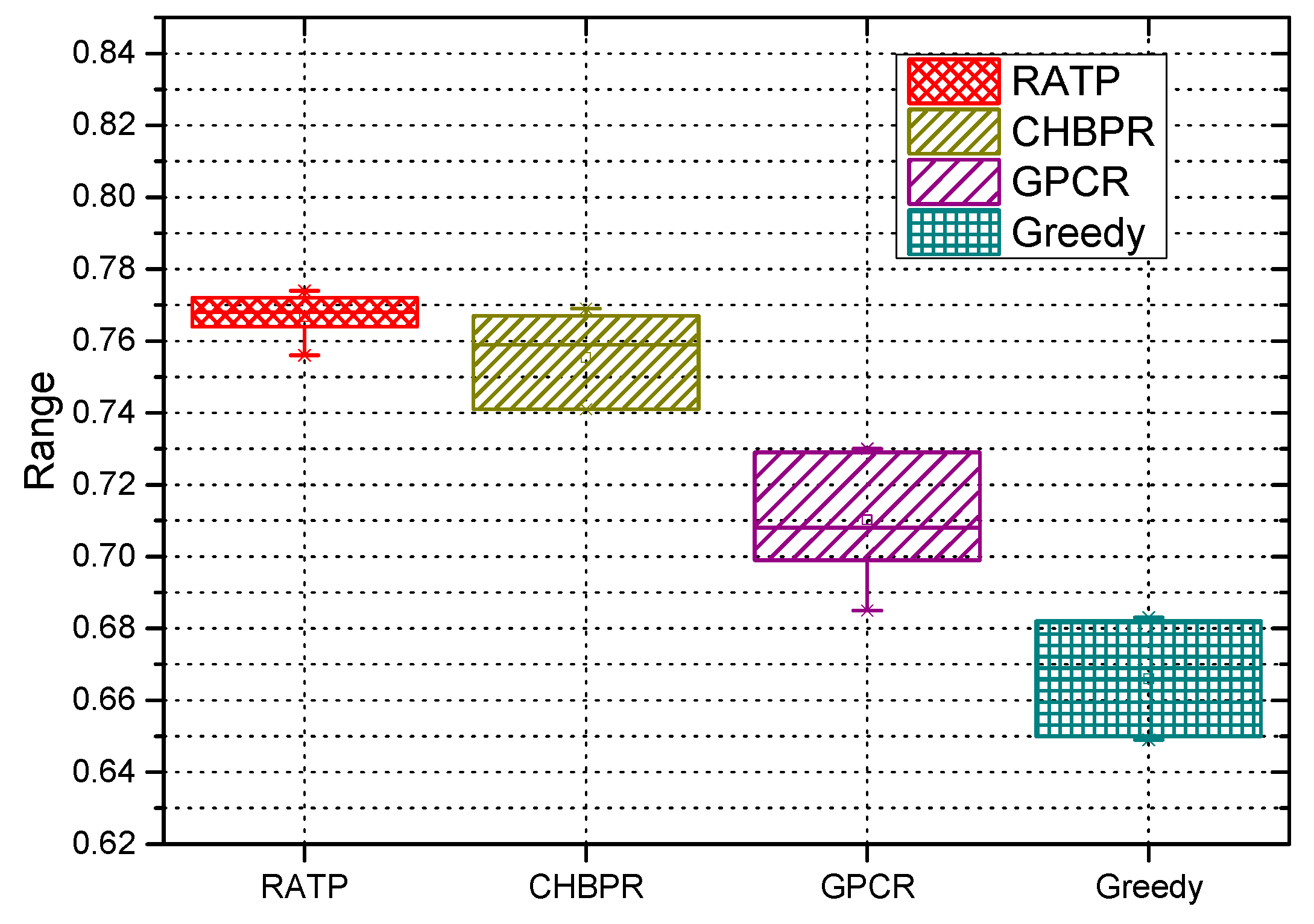
4.1. Performance Measurement Parameters

In order to better verify the performance of the RATP algorithm, the following metrics are used for evaluation:
RMSE: It is used to calculate the geometrical space error between the real and the predicted position, that is, the geometric space errors between the predicted trajectory points and the actual trajectory points.
R M S E = 1 N j = 1 N ( r e a l j p r e d j ) 2
where r e a l j is the real location ( x r e a l , y r e a l ) , p r e d j is the predicted location ( x p r e d , y p r e d ) , and N is the number of predicted trajectory points.
Delivery ratio: The number of packets successfully received by all the destination nodes in the network accounts for the ratio of the number of packets sent by the source node within a certain time. The higher the value, the higher the transmission success rate in the network.
End-to-end delay: The end-to-end delay is the average time that packets takes place from the initial node to the destination node.
Routing overhead: The total number of forwarded packets (FoM) minus the number of packets successfully received by the destination node (ReM), and then divided by the number of packets successfully received by the destination node. The formula is as follows:
R O R = F o M R e M R e M

4.2. Results and Discussion

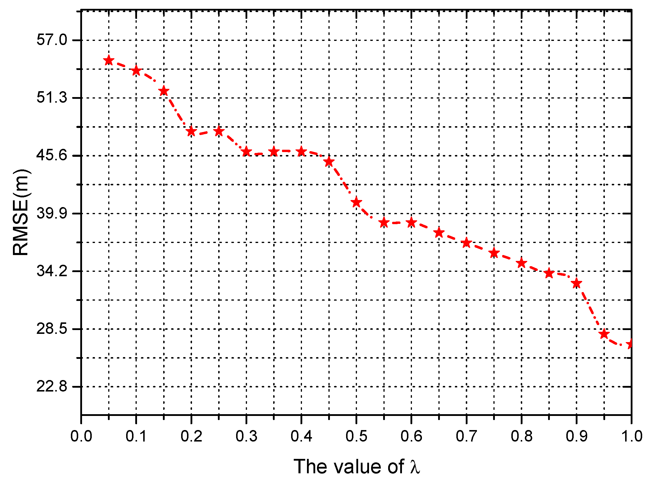
4.2.1. Prediction Error Analysis

Aiming at the simulation experiment, the performance of the algorithm is analyzed. The influence of different mobile coordination factors on error RMSE is introduced.
As shown in Figure 2, as the value of λ increases, the RMSE error gradually decreases. When the value of λ is greater than 0.75, RMSE shows a slow growth trend. The λ represents the node’s mobile performance. In real life, the movement of the node requires a corresponding time to adapt to the mobile coordination performance. As can be seen from Figure 2, the value has a certain influence on predicting the speed probability of the next moment. Therefore, it is not that the greater the value of λ , the better the performance of the algorithm.

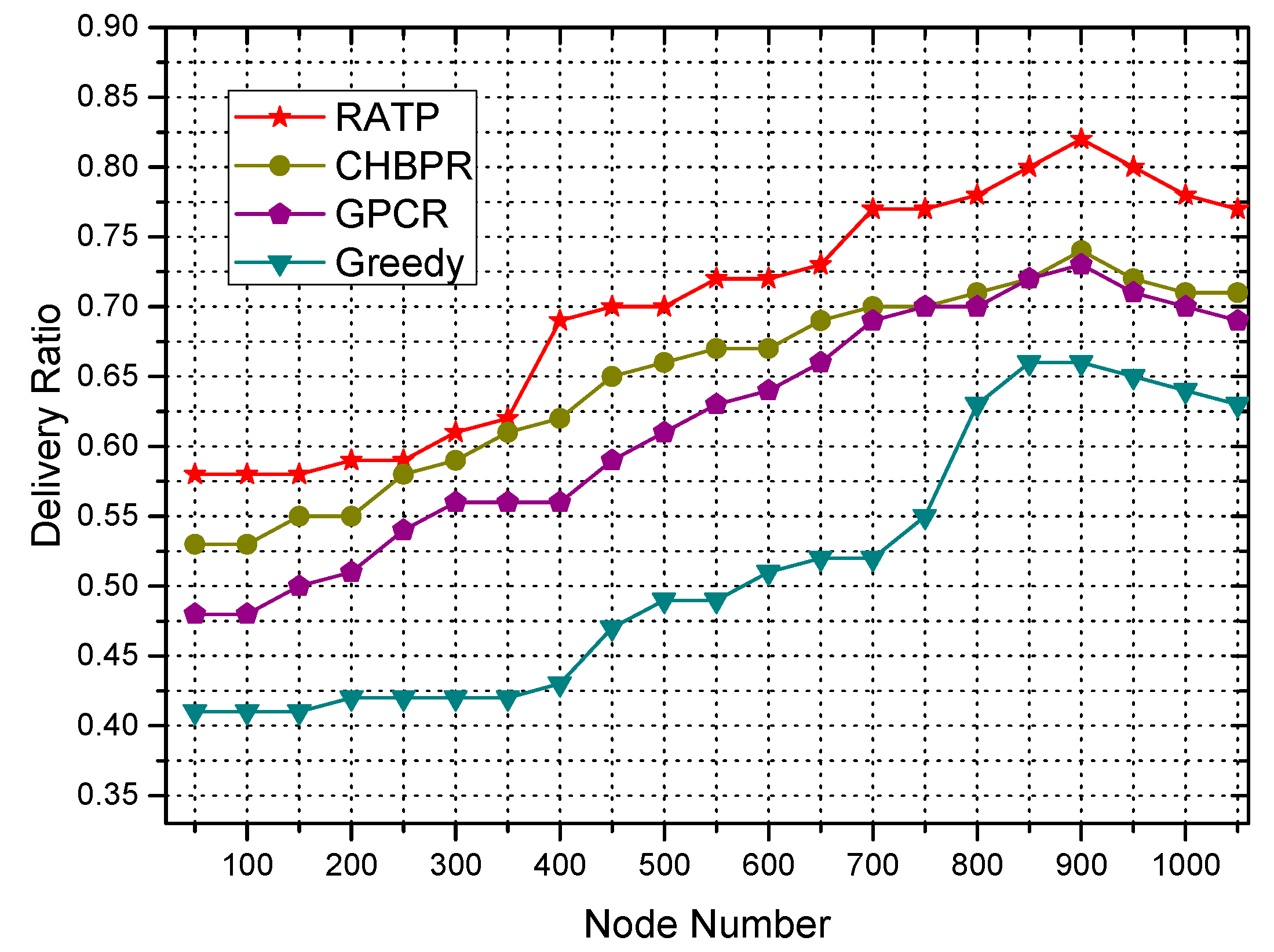
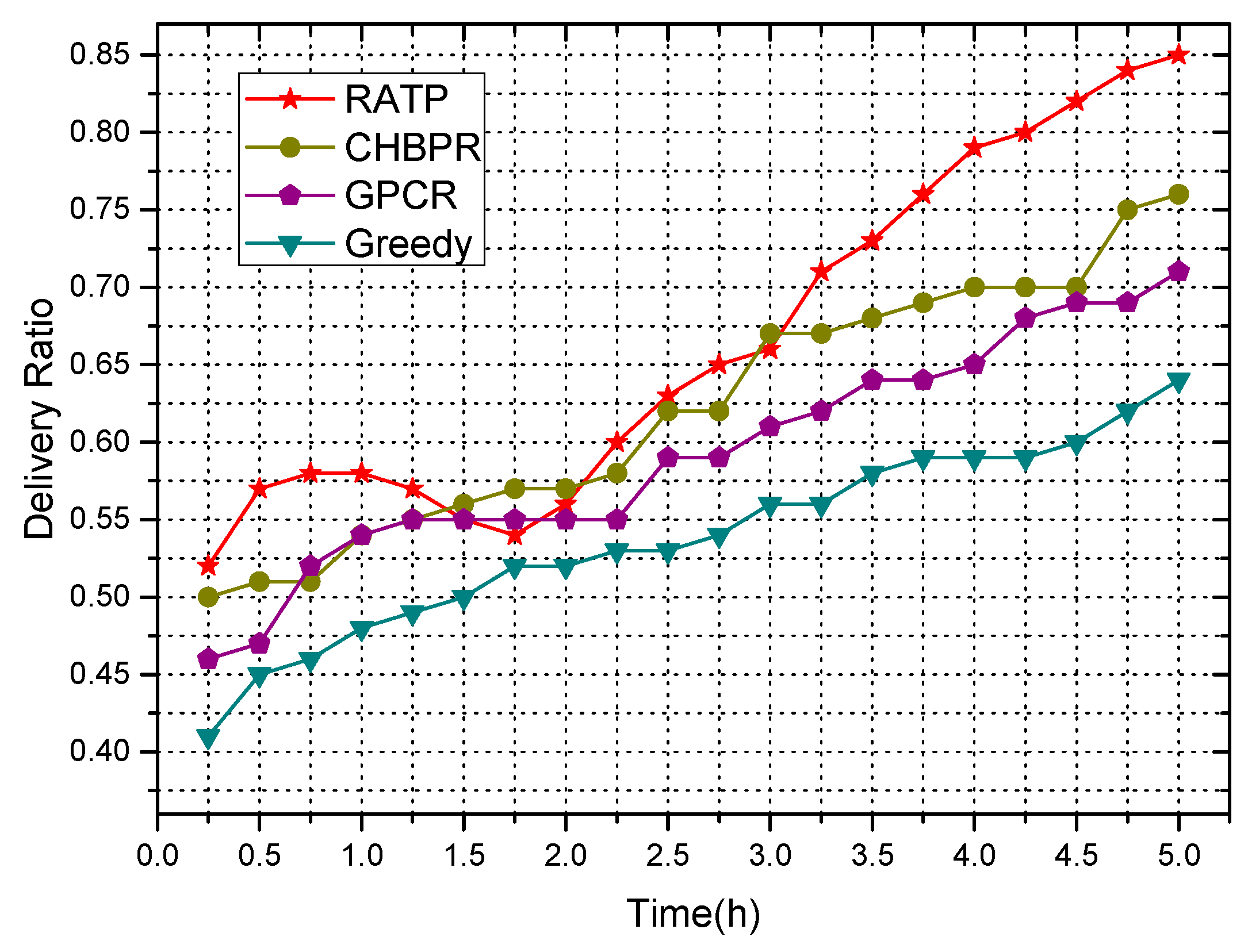
4.2.2. Delivery Ratio

This part mainly analyzes the performance of data delivery ratio of different algorithms. The change law of data delivery ratio with simulation time length is introduced. Additionally, the effect of the number of nodes on the data delivery ratio is studied.
In the same simulation scenario mode, the delivery ratio performance of different algorithms is studied. For the simulation results of each algorithm, we can find that the following Figure 3 mainly has five signs (max, the third quartile, median, the first quartile and min). As shown in Figure 3, in some special cases, two or more signs have very similar values. For example, the algorithm RATP proposed in this paper, the third quartile and median values are roughly around 0.01, which is very close. As can be seen from the Figure 3, although CHBPR has a high delivery ratio, it only considers the density of nodes and does not consider the distribution relationship between nodes, resulting in poor connectivity, making the data unable to be more efficient and rapid transport to the destination node, delivery ratio decline. Compared with other algorithms, the RATP algorithm has a higher delivery ratio because the algorithm not only analyzes the different location probabilities, but also analyzes the positional relationship among the node at the same time, the better the connectivity of selected routes, the delivery ratio is higher.
Figure 4 shows the data delivery ratio of the RATP algorithm, CHBPR algorithm, GPCR algorithm and Greedy algorithm under different simulation times. It can be seen from the figure that as the simulation time increases, the data delivery ratio of the four algorithms also increases. The experimental results show that the RATP algorithm has a low data delivery ratio when the simulation time is between 1.5 h and 2.5 h. This is because a large amount of data is dropped, causing congestion in the network. However, RATP still has a higher data delivery ratio than other algorithms.
Figure 5 shows the data delivery ratio of the RATP algorithm, CHBPR algorithm, GPCR algorithm and Greedy algorithm under different node numbers. As can be seen from Figure 5, as the number of nodes increases, the RATP algorithm has a higher data delivery ratio than other algorithms. The simulation results show that when the number of nodes is within a certain range, the data delivery ratio increases with the number of nodes. As the number of nodes increases, the chances of encountering between nodes increases, network connectivity increases, and information transmission efficiency increases. However, when the number of nodes exceeds a certain range, the number of neighbor nodes increases due to the increase of the node density, thereby increasing the probability of the selected next-hop node, and finally the data delivery ratio is lowered.

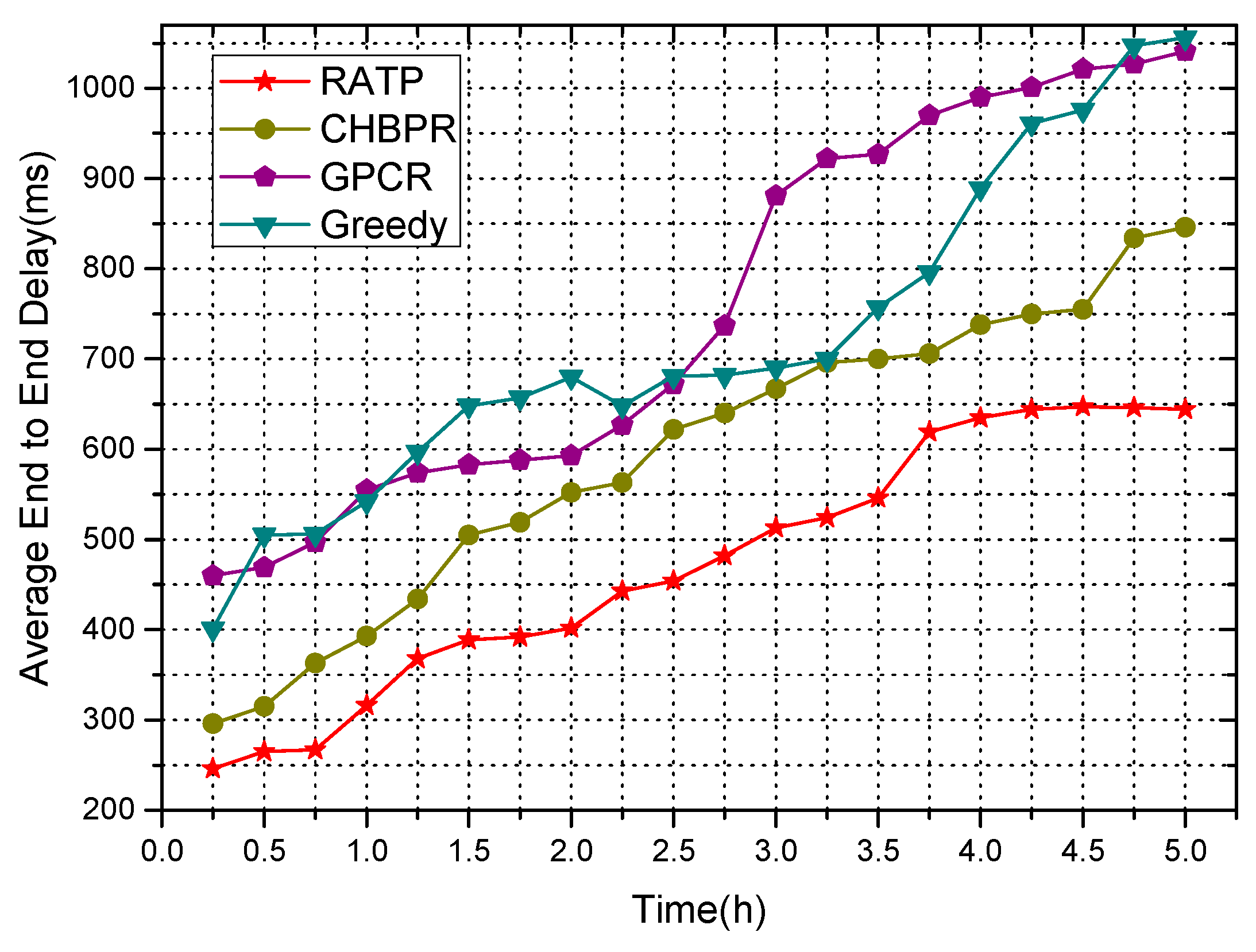
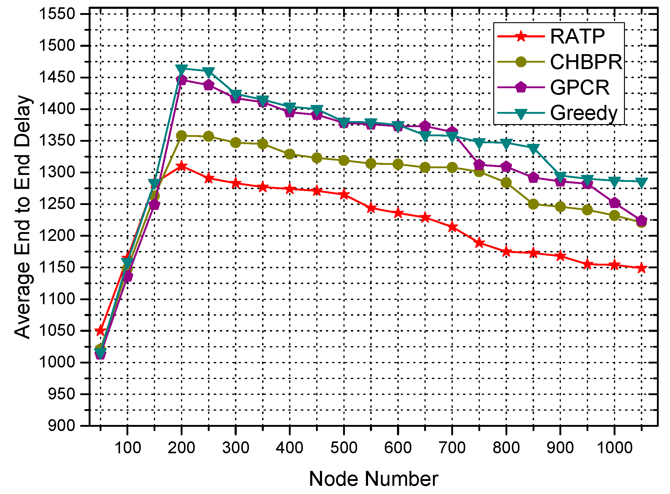
4.2.3. End-to-End Delay

This section mainly analyzes the average end-to-end delay performance of four different algorithms. The change law of average end-to-end delay with simulation time length is introduced and the effect of the number of nodes on the average end-to-end delay is studied.
Figure 6 shows the average end-to-end delay of the RATP algorithm, CHBPR algorithm, GPCR algorithm and Greedy algorithm under different simulation times. It can be seen from the figure that as the simulation time increases, the average end-to-end delay of the four algorithms also increases. This is because, as the simulation time increases, the number of packets in the network increases, and the entire network takes more time to process, resulting in an increase in data transmission delay. In any case, the RATP algorithm average end-to-end delay is significantly slower than the other three algorithms.
Figure 7 shows the average end-to-end delay of the RATP algorithm, CHBPR algorithm, GPCR algorithm and Greedy algorithm under different node numbers. It can be seen from the figure that as the number of nodes increases, the average end-to-end delay of the four algorithms increases first and then decreases. When the number of nodes is small, the selected forwarding node is far away, resulting in an increase in data transmission delay. When the number of nodes reaches a certain level, the number of forwarding nodes in the network increases, the data transmission time is relatively reduced, and the transmission delay is relatively reduced. Compared with the other three algorithms, the RATP algorithm has the lowest average end-to-end delay. This is because the RATP analyzes the distribution of the entire network node and the global information of the network, making the selected routing more connected, the higher the reliability and real-time, the lower the delay.

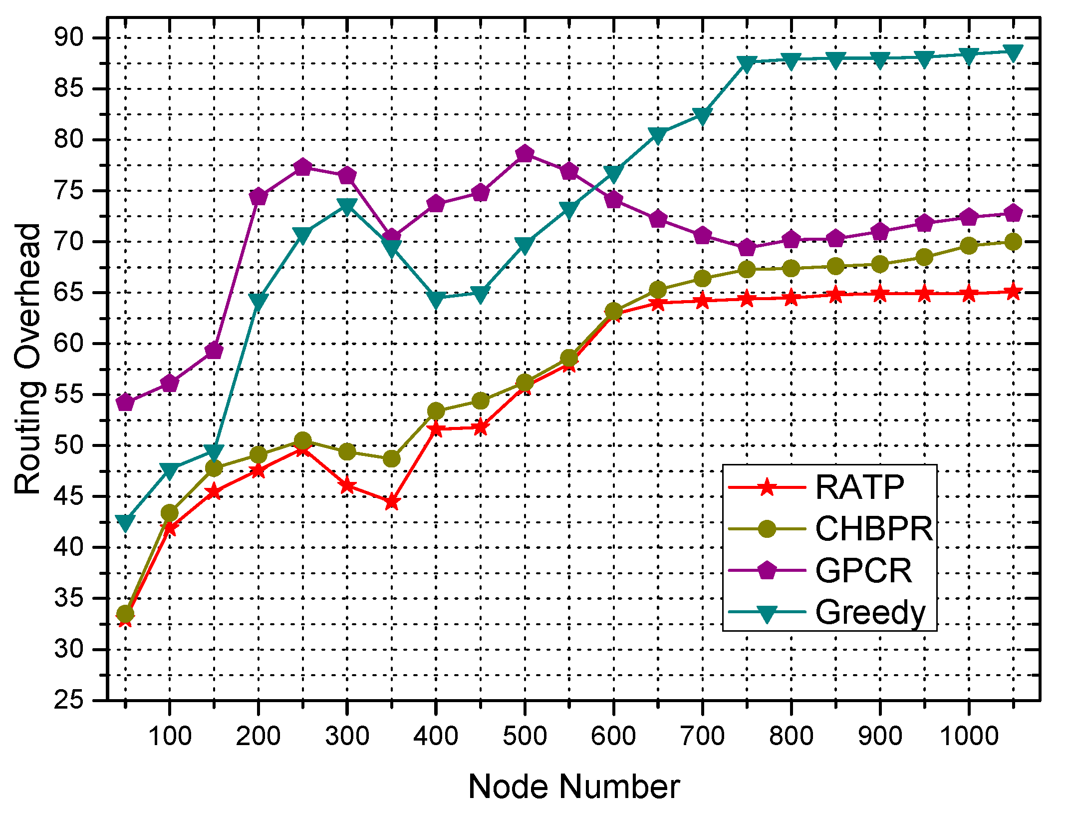
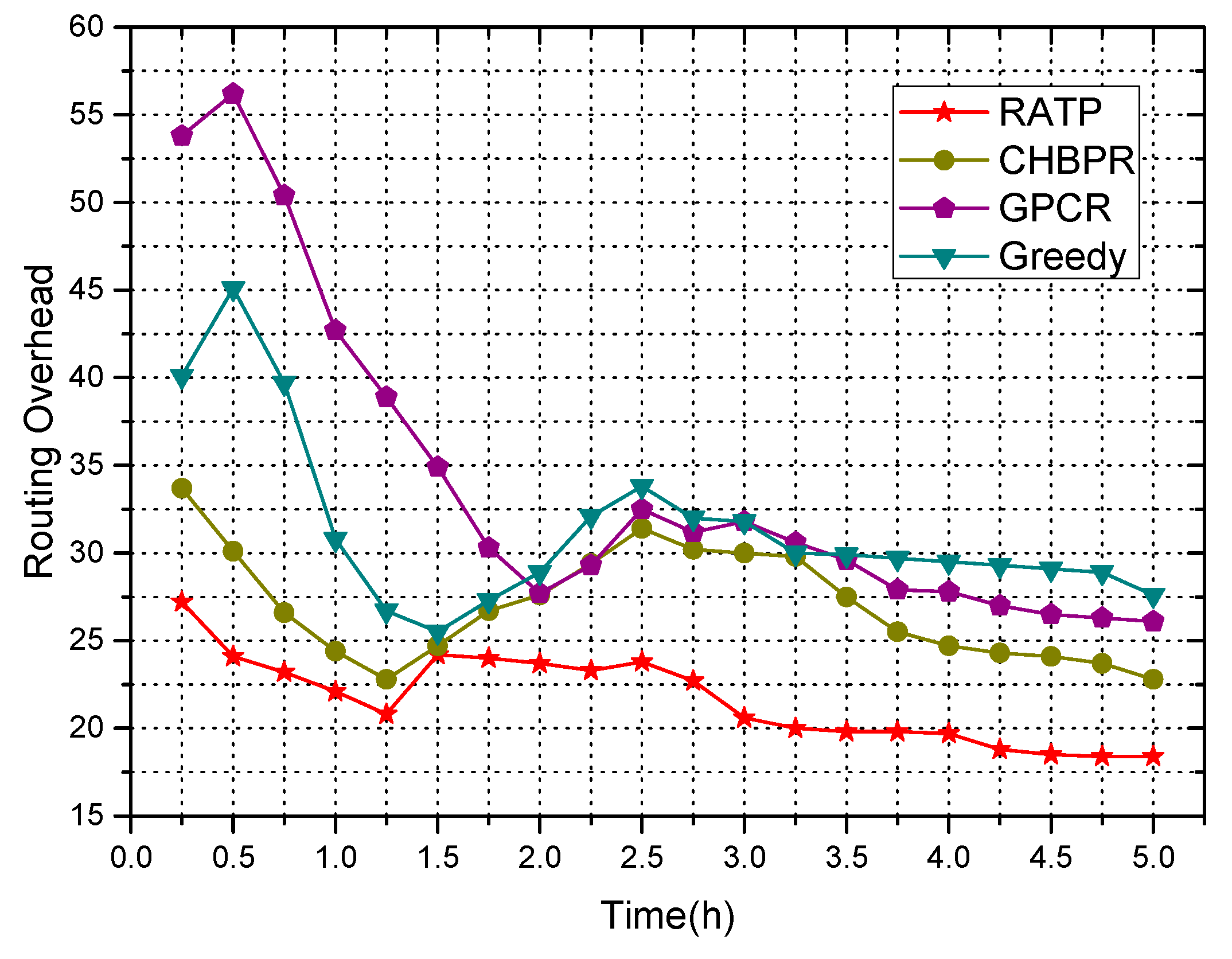
4.2.4. Routing Overhead

This section mainly analyzes the performance of the routing overhead of the four different algorithms. The change law of routing overhead with simulation time length is introduced. Additionally, the effect of the number of nodes on the routing overhead is studied.
Figure 8 shows the routing overhead of the RATP algorithm, the CHBPR algorithm, the GPCR algorithm, and the Greedy algorithm at different simulation times. It can be seen from the figure that as the simulation time increases, the routing overhead of the four algorithms presents an unstable state. The RATP algorithm selects the next-hop data forwarding node by analyzing the node moving position. When the information is forwarded to the next-hop node, it can sense the location information of other nodes in advance and forward the information to the appropriate node. Therefore, path discovery time is reduced, routing overhead is reduced, and route cost changes are more stable than other algorithms.
Figure 9 shows the routing overhead of the RATP algorithm, CHBPR algorithm, GPCR algorithm, and Greedy algorithm under different node numbers. It can be seen from the figure that as the number of nodes increases, the routing overhead of the four algorithms increases gradually. This is because when the number of nodes increases, the path propagation fails more frequently. As a result, the number of nodes passing through the message increases relatively and the path is found to be relatively slow. Since the RATP algorithm can further select the information forwarding path by analyzing the location information of the node, the algorithm can obtain other mobile node location information in advance and select an appropriate node to forward the information, so the routing cost is lower than other algorithms.

5. Conclusions

The opportunistic network has the characteristics of topological dynamics and bandwidth first. The good routing protocol is the primary problem of constructing the opportunistic network, and it is also a hotspot and a difficult point of research. This paper proposes a routing algorithm based on trajectory prediction (RATP). The RATP algorithm uses the Gaussian process to calculate the probability of the node’s future time velocity by analyzing the historical trajectory characteristics of the node. According to the predicted location information, the candidate node metric value is calculated and the node with the smaller metric value is selected as the data forwarding node, which effectively reduces the packet loss rate of the boundary and avoids excessive consumption of the edge node. The simulation results show that compared with other algorithms, the algorithm has higher transmission success rate, and the transmission delay and routing overhead are significantly reduced.
In future work, first of all we hope to realize the position prediction algorithm and routing protocol in practical applications, and verify the effectiveness of the prediction algorithm and routing protocol in this paper by using real application scenarios. Secondly, we hope to consider the constrained factors of more nodes, so as to select a better forwarding node to achieve higher routing performance.

Author Contributions

Conceptualization, Methodology, Analysis, Investigation, Writing—original draft preparation, Writing—review and editing, Visualization, P.Z., L.W. and J.W.; Supervision, Project Administration, Funding Acquisition, M.Z.

Funding

This research was funded by the National Natural Science Foundation of China (No.61572526).

Conflicts of Interest

The authors declare no conflicts of interest.

References

  1. Halikul, L.; Mohamad, A. EpSoc: Social-Based Epidemic-Based Routing Protocol in Opportunistic Mobile Social Network. Mob. Inf. Syst. 2018, 2018, 6462826. [Google Scholar]
  2. Wu, J.; Chen, Z.; Zhao, M. Weight distribution and community reconstitution based on communities communications in social opportunistic networks. Peer-to-Peer Netw. Appl. 2008, 12, 158–166. [Google Scholar] [CrossRef]
  3. Huang, F. Research on a Location-Based Routing Protocol E-LAR in Mobile Ad Hoc Networks. Master’s Thesis, Central South University, Changsha, China, June 2009. [Google Scholar]
  4. Li, J.; Jannotti, J.; De Couto, D.S.; Karger, D.R.; Morris, R. A scalable location service for geographic ad hoc routing. In Proceedings of the 6st Annual International Conference on Mobile Computing and Networking, Boston, MA, USA, 6–11 August 2000; pp. 120–130. [Google Scholar]
  5. Wang, L.L.; Chen, Z.G.; Wu, J. Vehicle trajectory prediction algorithm in vehicular network. Wirel. Netw. 2018, 1–14. [Google Scholar] [CrossRef]
  6. Wu, J.; Chen, Z. Human Activity Optimal Cooperation Objects Selection Routing Scheme in Opportunistic Networks Communication. Wirel. Pers. Commun. 2017, 95, 3357–3375. [Google Scholar] [CrossRef]
  7. Pozza, R.; Nati, M.; Georgoulas, S.; Moessner, K.; Gluhak, A. Neighbor discovery for opportunistic networking in internet of things scenarios: A survey. IEEE Access 2015, 3, 1101–1131. [Google Scholar] [CrossRef]
  8. Li, Z.; Shen, H.Y.A. Direction Based Geographic Routing Scheme for Intermittently Connected Mobile Networks. In Proceedings of the 8th International Conference on Embedded and Ubiquitous Computing, Shanghai, China, 17–20 December 2008; pp. 359–365. [Google Scholar]
  9. Ko, Y.B.; Vaidya, N.H. Location·aided routing (LAR) in mobile ad hoe networks. Wirel. Netw. J. 2000, 6, 307–321. [Google Scholar] [CrossRef]
  10. Wu, K.; Harms, J. Location trace aided routing in mobile ad hoe networks. In Proceedings of the 9th Intemational Conference on Computer Communications and Networks, Las Vegas, NV, USA, 16–18 October 2000; pp. 354–359. [Google Scholar]
  11. Karp, B.; Kung, H.T. GPSR: Greedy perimeter stateless routing for wireless networks. In Proceedings of the 6th Annual International Conference on Mobile Computing and Networking, Boston, MA, USA, 6–11 August 2000; pp. 243–254. [Google Scholar]
  12. Huang, C. The Simulation of Grid Location Service Routing Protocol Mobile Ad Hoc Networks. Master’s Thesis, Xidian University of Electronic Technology, Xi’an, China, June 2007. [Google Scholar]
  13. Stavroulaki, V.; Tsagkaris, K.; Logothetis, M.; Georgakopoulos, A.; Demestichas, P.; Gebert, J.; Filo, M. Opportunistic Networks. IEEE Veh. Technol. Mag. 2011, 6, 52–59. [Google Scholar] [CrossRef]
  14. Lin, C.R.; Gerla, M. Adaptive clustering for mobile wireless networks. IEEE J. Sel. Areas Commun. 1997, 15, 1265–1275. [Google Scholar] [CrossRef]
  15. Tsiropoulou, E.E.; Mitsis, G.; Papavassiliou, S. Interest-aware energy collection & resource management in machine to machine communications. Ad Hoc Netw. 2018, 68, 48–57. [Google Scholar]
  16. Tsiropoulou, E.E.; Paruchuri, S.T.; Baras, J.S. Interest, energy and physical-aware coalition formation and resource allocation in smart IoT applications. In Proceedings of the 2017 51st Annual Conference on Information Sciences and Systems (CISS), Baltimore, MD, USA, 22–24 March 2017; pp. 1–6. [Google Scholar]
  17. Basagni, S.; Chlamtac, I.; Syrotiuk, V.R.; Woodward, B.A. A distance routing effect algorithm for mobility (DREAM). In Proceedings of the 4th Annual ACM/IEEE International Conference on Mobile Computing and Networking, Dallas, TX, USA, 25–30 October 1998; pp. 76–84. [Google Scholar]
  18. Bamrah, A.; Woungang, I.; Barolli, L.; Dhurandher, S.K.; Carvalho, G.H.; Takizawa, M. A Centrality-Based History Prediction Routing Protocol for Opportunistic Networks. In Proceedings of the International Conference on Complex, Intelligent, and Software Intensive Systems (CISIS), Fukuoka, Japan, 6–8 July 2016. [Google Scholar]
  19. Dhurandher, S.K.; Woungang, I.; Rajendra, A.; Ghaie, P.; Chatzimisios, P. A Centrality-based ACK Forwarding Mechanism for E_cient Routing in Opportunistic Networks. In Proceedings of the International Conference on Cyber Physical Systems, IoT and Sensors Networks (Cyclone 2015), Rome, Italy, 26 October 2015. in press. [Google Scholar]
  20. Yu, Y.; Govindan, R.; Estrin, D. Geographic and Energy-Aware Routing: A Recursive Data Dissemination Protocol for Wireless Sensor Networks; UCLA Computer Science Department Technical Report; UCLA Computer Science Department: Los Angeles, CA, USA, 2001. [Google Scholar]
  21. Kamal, J.M.M.; HASAN, M.; Griffiths, A.; Yu, H. Prediction-based Opportunistic Greedy Routing for Vehicular Ad Hoc Networks. In Proceedings of the 16th International Conference on Automation and Computing, Birmingham, UK, 11 September 2010. [Google Scholar]
  22. Finn, G.G. Routing and Addressing Problems in Large Metropolitan-Scale Internetworks; ISI Research Report ISU/RR; Advanced Research Projects Agency (DOD): Washington, DC, USA, 1987. [Google Scholar]
  23. Zou, X.; Cao, Y.; Liu, X.; Gao, X. DPSO-Based Clustering Routing Approach for WSN. J. Wuhan Univ. 2008, 54, 99–103. [Google Scholar]
  24. Lochert, C.; Mauve, M.; Füßler, H.; Hartenstein, H. Geographic routing in city sce-narios. Mob. Comput. Commun. Rev. 2005, 9, 69–72. [Google Scholar] [CrossRef]
  25. Jerbi, M.; Meraihi, R.; Senouci, S.M.; Ghamri-Doudane, Y. GyTAR: Improved greedy traffic aware routing protocol for vehicular ad hoc networks in city environments. In Proceedings of the International Workshop on Vehicular Ad Hoc Networks, Los Angeles, CA, USA, 29 September 2006; pp. 88–89. [Google Scholar]
Figure 1. The metric of each node.
Information 10 00049 g001
Figure 2. RMSE vs value of λ.
Information 10 00049 g002
Figure 3. Delivery Ratio.
Information 10 00049 g003
Figure 4. Delivery Ratio vs simulation time.
Information 10 00049 g004
Figure 5. Delivery Ratio vs number of nodes.
Information 10 00049 g005
Figure 6. End-to-end delay vs number of nodes.
Information 10 00049 g006
Figure 7. End-to-end delay vs number of nodes.
Information 10 00049 g007
Figure 8. Routing overhead vs number of nodes.
Information 10 00049 g008
Figure 9. Routing overhead vs. number of nodes.
Information 10 00049 g009

