Article

Dense Model for Automatic Image Description Generation with Game Theoretic Optimization

Department of Computer Science, Cochin University of Science and Technology, Kochi, Kerala 682022, India
*
Author to whom correspondence should be addressed.
Information 2019, 10(11), 354; https://doi.org/10.3390/info10110354
Submission received: 11 October 2019 / Revised: 9 November 2019 / Accepted: 13 November 2019 / Published: 15 November 2019
(This article belongs to the Section Artificial Intelligence)

Abstract

:
Due to the rapid growth of deep learning technologies, automatic image description generation is an interesting problem in computer vision and natural language generation. It helps to improve access to photo collections on social media and gives guidance for visually impaired people. Currently, deep neural networks play a vital role in computer vision and natural language processing tasks. The main objective of the work is to generate the grammatically correct description of the image using the semantics of the trained captions. An encoder-decoder framework using the deep neural system is used to implement an image description generation task. The encoder is an image parsing module, and the decoder is a surface realization module. The framework uses Densely connected convolutional neural networks (Densenet) for image encoding and Bidirectional Long Short Term Memory (BLSTM) for language modeling, and the outputs are given to bidirectional LSTM in the caption generator, which is trained to optimize the log-likelihood of the target description of the image. Most of the existing image captioning works use RNN and LSTM for language modeling. RNNs are computationally expensive with limited memory. LSTM checks the inputs in one direction. BLSTM is used in practice, which avoids the problem of RNN and LSTM. In this work, the selection of the best combination of words in caption generation is made using beam search and game theoretic search. The results show the game theoretic search outperforms beam search. The model was evaluated with the standard benchmark dataset Flickr8k. The Bilingual Evaluation Understudy (BLEU) score is taken as the evaluation measure of the system. A new evaluation measure called GCorrectwas used to check the grammatical correctness of the description. The performance of the proposed model achieves greater improvements over previous methods on the Flickr8k dataset. The proposed model produces grammatically correct sentences for images with a GCorrect of 0.040625 and a BLEU score of 69.96%

1. Introduction

The World Wide Web is a data store with a vast collection of images. Image searching is a challenging task. Currently, most of the search engines use meta-data to search for images. The metadata of images includes user annotated tags, surrounding text, captions, etc. Not every picture on the Internet has metadata. Therefore, the automatic generation of image descriptions reduces the complexity of image searching. The applications range from supporting visually impaired users to human–robot interaction.
The depiction of an image contains scenes, specific objects, spatial relationships, and attributes for adding additional information about objects. The output of computer vision combined with language models is suitable for the image description generation process. Natural language Generation (NLG) is one of the basic research issues in Natural Language Processing (NLP). It has a broad range of applications in machine translation, discourse, summarization, and machine assisted vision. Regardless of the significant progress in the most recent decade, NLG remains an open research issue. Previous sentence generation was done by either utilizing an n-gram language model or template based approach. As of now, RNN (Recurrent Neural Network) [1] and LSTM [2] are connected for NLG.
The essential steps of automatic image description generation are image parsing and surface realization. Image parsing is the process of generating features of the image. Surface realization is the process of generating an image description. The task of surface realization is to create relevant, understandable, and question specific content reports. Image parsing is done using a deep convolutional neural network. Deep recurrent neural systems are utilized for surface realization. The optimization, such as word selection, is done using two methods, game theoretic search and beam search. To describe an image effectively, all entities, attributes, and relationships are identified in the sentence and mapped to the complex visual scene.
Google’s Neural Image Caption generator (Google NIC) [3] was used as the seminal paper for writing this paper. The NIC model used an encoder-decoder framework in which the encoder was InceptionV3 and the decoder was the recurrent neural network. Another important work was Andrej Karpathy’s work [4] from Stanford University. The objective of the work was to generate a human readable image description using past and future contexts of trained captions. The proposed model differed from existing models in that it learned the semantics of the sentences using BLSTM’s bidirectional nature and mapped sentence features to complex image features.
To achieve this objective, a framework for the automatic generation of image descriptions with two major components was proposed. They are explained as follows:
  • Image parsing:
    Image parsing is done using Densenet. The advantages of using Densenet are as follows: elimination of the vanishing gradient problem, reinforcing feature propagation, supporting feature reuse, and reducing the number of parameters.
  • Surface realization:
    Two BLSTMs are used to implement surface realization. First, BLSTM is implemented for language modeling and the other for caption generation. The significance of BLSTM is that it investigates the past and future reliance to give a forecast. Earlier, the word selection in caption generation was performed using beam search. In our work, beam search and game theoretic search are implemented, and it is found that game theoretic search outperforms beam search.
A grammatical accuracy measure called GCorrectis used to evaluate the grammatical correctness of the generated description.
The paper is structured as follows. A review of the existing works is discussed in Section 2. Section 3 explains the mathematical foundation of the proposed model. The implementation and experiment results are explained in Section 5 and Section 6. The paper is concluded in Section 7.

2. Related Work

Automatic image description generation is a core part of image understanding. Several approaches have been developed for this task. These systems are categorized based on the generation methods and image feature extraction methods. Different kinds of image captioning systems are discussed in Section 2.1. The image captioning systems became more advanced after the deep learning models become popular for object detection. The deep neural networks are a powerful tool for image feature extraction and are explained in Section 2.2.

2.1. Image Captioning

Image description generation models are categorized into three types. These are direct generation models, visual space retrieval models, and multimodal space retrieval models [5]. The general approach of the direct generation model is to predict the semantics of the image using the visual features first and then to generate sentences corresponding to these semantics. Midge [6] and BabyTalk [7] are based on direct generation models. In the visual space retrieval model, the portrayal is created by retrieving similar images and transferring captions from the visual space to a new image. The Im2Textmodel [8] uses this approach. The multimodal space retrieval model treats the description problem as a ranking problem. The methods of Hodosh et al. [9], Socher et al. [10], and Karpathy et al. [4] followed this approach. Some image captioning systems use a visual attention mechanism [11].
Image captioning systems can be classified into two types based on the feature extraction methods. They are layout based approaches and deep neural network based approaches.

2.1.1. Layout Based Approaches

In this approach, the captions are generated using the outputs of object detection, attributes, and scene identification. Farhadi et al. [12] used the Markov random field, GIST, and Support Vector Machine (SVM) for caption generation and converted the scene elements to text using layout. Kulkarni et al. [7] utilized the Conditional Random Field (CRF) to associate the objects, attributes, and prepositions. Midge [6] utilized the Berkeley parser and Wordnet ontologies to generate text. The disadvantage of these systems is the generation of incorrect captions due to inaccurate object detection. These systems used traditional machine learning algorithms for object detection, which resulted in poor performance.

2.1.2. Deep Neural Network Based Approaches

The image captioning system involves image to text translation. Currently, most of the image captioning systems adopt the encoder-decoder framework. The image feature extraction is done in the encoding phase. The encoding is done using deep neural networks, which give better performance in object detection. The decoder is implemented using recurrent neural networks or LSTM, which is used for caption generation. Kiros et al. [13] used feed-forward neural networks and multimodal log-bilinear models to generate words from previous words. Some systems utilized the recurrent neural network for caption generation. Gong et al. [14] used deep CNN and bag of words for description generation. Karpathy [15] utilized Region level CNN (RCNN) and bidirectional RNN for whole description generation. Vinyal et al. [3] used LSTM as a decoder. Donnelly et al. [16] produced a multimodal architecture for caption generation. Sou et al. [17] provided linguistic importance to the interaction between learned word embeddings and the LSTM hidden states. Wang et al. [18] built a deep Convolutional Neural Network (CNN) and two separate LSTM networks for caption generation. You et al. [19] used top-down and bottom-up approaches for image captioning.
Top-down visual attention mechanisms are commonly used in image captioning. Peter Anderson’s method [20] was based on a hybrid of the top-down and bottom-up visual attention mechanism. Agashi Poghosyan [21] modified the LSTM cell to get greater significance of image features. The convolutional image captioning [22] system uses convolutional networks for captioning. The Groupcap system [23] considers the diversity of image captions. Phi-LSTM [24] predicts image captions from phrase to sentence. Han’s system [25] used a fast image captioning system using YOLO and LSTM. Text based visual attention has also been implemented in image captioning systems [26].

2.2. Deep Neural Network

Currently, deep neural networks have an important role in caption generation. Deep convolutional neural networks [27] are feed-forward neural networks with a convolution operation instead of multiplication. The disadvantage of deep CNN is the difficulty in training due to the vanishing gradient problem. The variants of deep CNN are LeNet [28], AlexNet [29], VGGNet [30], GoogLeNet [31], Residual Neural Network (ResNet) [32], highway network [33], Densenet [34], MobileNet [35], SqueezeNet [36], etc. VGGNet was developed and trained by the Visual Geometry Group (VGG) at the University of Oxford. ResNets have shortcut connections parallel to convolutional layers. The gradients are backpropagated through shortcut connections. Therefore, ResNet has no vanishing gradient problem, and thus, the training is faster. Recurrent Neural Networks (RNN) [1] and long short-term memory are used for sentence generation. RNNs are good for short contexts because they manage short term dependencies and have the vanishing gradient problem. Long haul expectations are hard for RNN. Therefore, LSTMs come into the picture. They consider long term dependencies for sequence prediction. A word embedding is a learned description of text where similar kinds of words have the same representation. It is also a technique for representing words in a vector form using a predefined vector space. It also shows the progress of deep learning in solving challenging natural language problems. The examples of word embedding models are bag of words, TF-IDF, distributed embeddings, embedding layer, Word2vec [37], GloVe [38], and FastText [39]. Bag of words, TF-IDF, and distributed embeddings are traditional word embedding models. Word2Vec, GloVe, and FastText are neural network based word embeddings.

2.3. Game Theory

Game theory [40] is a branch of mathematics that models the conflicts and coordination between different players in a scenario. In game theory, a problem is formulated as a game. The game can be cooperative and non-cooperative. In the non-cooperative game, individual players are the decision-makers, and so, they do not make alliances with other players in the game. The critical concept in non-cooperative game theory is the Nash equilibrium, which was introduced by John Forbes Nash. Cooperative games are games in which coalitions between players result in profits in the game.

Cooperative Game Theory

Cooperative games are games in which players should form alliances due to cooperative behavior. The main difference between cooperative and non-cooperative games is that coalitions are formed between players. These games are mathematically defined with a value function v : 2 N R , where Nis the number of players. The measures such as the Shapley value and core value determine the payoffs for players in each coalition [41]. Sun [41] developed a feature selection method using cooperative game theory. In this work, cooperative game theory is used.

3. System Architecture

Let I be the image and D be the description that is represented as < D 1 , D 2 , D 3 , D n > , and the proposed model optimizes the log-likelihood of description D given image I. The parameters of the model can be expressed as θ * = l o g P ( D n | I ; D 1 , D 2 D n 1 ) . In this model, for each iteration, the probabilities of each word in the vocabulary is calculated.
The architecture of the proposed model is depicted in Figure 1. The proposed model is a combination of the image model, language model, and caption model, which are explained in Section 3.1, Section 3.2 and Section 3.3. The inputs to the model are the image and a partial caption. The image is a numerical array of size 224 × 224 × 3 , and the partial caption is a numerical vector of length 40. The image model encodes the image as features of size 40 × 128 . The language model converts the image description into an encoded vector of sentence features. CNN in the image model encodes the image into features, and BLSTM in the caption model produces the next word from the image features and sentence features. The caption model initially computes the log probability of the words in the vocabulary, selects the word using game theoretic search and beam search, and generates the description of the image.

3.1. Image Model

The image model extracts the features of the image and reduces the size of the image features. The important components of the image model are Densenet [34], the dense layer, the activation layer, and the repeat layer. Figure 2 explains the architecture of the image model.

3.1.1. Densenet

Densenet was used to extract the visual content of the image. It is a type of deep convolutional neural network. In Densenet, the input of the l th layer is the output of all preceding layers and is expressed by Equation (4). It provides an excellent object classification rate. The architecture of Densenet is shown in Figure 3.
Equation (4) defines the operation of Densenet. The function D is a combination of convolution, batch normalization, and ReLU functions. Convolution is an element-wise multiplication of image and kernel matrices. Batch normalization is the operation of shifting inputs with zero mean and unit variance in each mini-batch. After that, the elements with negative values are converted to zero using the ReLU function.
D e n s e n e t ( I ) = D l ( [ I , f 1 , f 2 , f l 1 ] )
where I is the image and f 1 , f 2 , f l 1 are the features of the first, second, and l 1 th layers, respectively.
Densenet was used as the image feature encoder to get the spatial representation of images. In the experiments, the image model used Densenet with 161 layers. The input of Densenet had dimensions of 224 × 224 × 3 , which represent the dimensions of the image. The output of the last layer of Densenet had a dimension of 2208 in this work.

3.1.2. Dense Layer

This was a fully connected neural network layer for feature reduction. The input of this layer was features extracted from Densenet. This layer reduced the feature size from 2208 to 128. The output of the dense layer ( x 1 ) is defined by Equation (2).
x 1 = W d · D e n s e n e t ( I )
where W d is a kernel weights matrix having dimensions of 128 × 2208 .

3.1.3. Activation Layer

The output of the dense layer was applied to the activation layer to get a fixed size positive vector using the ReLU function. The ReLU function replaced negative values with zeros in the input. Equation (3) defines the functionality of this layer.
R e L U ( x ) = m a x ( 0 , x )

3.1.4. Repeat Layer

The repeat layer was used for repeating the data up to the maximum caption length for merging purposes, which is represented by Equation (4).
x 0 = r e p e a t ( x 1 , m a x _ c a p _ l e n )
where m a x _ c a p _ l e n is the maximum caption length.

3.2. Language Model

The caption was encoded as a vector of language features in the language model phase. The language model was implemented using the embed layer, Bidirectional LSTM (BLSTM) [18], and the time distributed dense layer. The architecture of the language model is shown in Figure 4.

3.2.1. Embed Layer

The captions were preprocessed and given to the embed layer. The functionality of the embed layer was to represent each word using a word embedding of size m a x _ c a p _ l e n × S i where S i is the fixed size of LSTM input and m a x _ c a p _ l e n is the maximum caption length. In the experiment, the value of S i was 256. The output of the embed layer was given to the BLSTM.

3.2.2. Bidirectional LSTM

Long Short Term Memory (LSTM) [2] is a type of recurrent neural network architecture that eliminates the vanishing gradient problem in RNN and allows for learning long term sequences. The memory blocks are in charge of recalling things, and control of this memory is done through three multiplicative units called gates. The gates are the input, forget, and output gates. The input gate is responsible for adding information to the cell state. The forget gate expels data from a cell state. The output gate functions to choose useful information from the current cell state as an outcome.
The BLSTM looks in the forward and backward direction of the caption. By examining the two paths, it utilizes the past and future information for modeling the current frame. The language model is described by the equation:
h L t = L S T M ( c t , h t 1 , m t 1 )
The BLSTM is a combination of forward and backward LSTMs. Therefore, L S T M is defined by using forward and backward LSTM equations. Forward LSTM is defined by the following equations.
f t = σ g ( k f c t + U f h t 1 + b f )
i t = σ g ( k i c t + U i h t 1 + b i )
o t = σ g ( k o c t + U o h t 1 + b o )
m t = f t m t 1 + i t σ m ( k m c t + U m h t 1 + b m )
h t = o t σ h ( m t )
Backward LSTM is defined by the following equations.
f t = σ g ( k f c t + U f h t + 1 + b f )
i t = σ g ( k i c t + U i h t + 1 + b i )
o t = σ g ( k o c t + U o h t + 1 + b o )
m t = f t m t + 1 + i t σ m ( k m c t + U m h t + 1 + b m )
h t = o t σ h ( m t )
where the initial values are m 0 = 0 , h 0 = 0 , and the operator ∘ denotes the Hadamard product. c t is the input vector to the LSTM unit; f t : activation vector of forget gates; i t : activation vector of input gates; o t : activation vector of output gates; h t is the output vector of the LSTM unit; m t is the cell state vector; K, U, and b are weight matrices and the bias vector, respectively; σ g is the sigmoid function; σ m and σ h are hyperbolic tangent functions.
In this work, the number of cells in BLSTM was the maximum caption length. The maximum caption length was set as 40. The output dimension of BLSTM was 40 × 512 .

3.2.3. Time Distributed Dense Layer

This is a time distributed fully connected layer, which means the operation is applied to every temporal slice of an input. This layer eases the burden of the network by limiting weights because one time step is prepared at once. This layer gives the sentence feature having a size of 40 × 128 .

3.3. Caption Model

The main components of the caption model are the merge layer, BLSTM, the dense layer, the softmax layer, beam search, and the caption generator. The outputs of the image and language models were merged using the row axis with the output having a size of 40 × 256 and given as the input to the caption model BLSTM.
Captions were modeled using bidirectional LSTM. The features of subtitles were fed to the model sequentially. The following equation defines BLSTM. It had 2000 features as the output.
The softmax function was used to calculate the score for each vocabulary item. The output of this layer was a vector containing the probability of each vocabulary item. It is described in Equation (16).
σ ( z ) j = e z j k = 1 K e z k for j = 1 , , K

Caption Generator

Game theoretic search and beam search are two algorithms implemented to find the right words for the description. The game theoretic search algorithm is described in Section 4. Beam search was used to find the right words for the description and the best description. It is an optimization of the best-first search algorithm. It is commonly used in machine translation systems to find the best translation. In beam search, a predetermined number of best partial solutions are taken as candidate solutions, and the predetermined number is called the beam size (width). In the experiment, a beamwidth of three was used. The words with the top three scores were taken for beam search, and partial solutions were obtained based on these words. The probability scores of each partial solutions were computed by adding the previous probability scores of the partial solution and the probability of each resultant word. The partial solutions with the top three scores were taken as the three best partial captions. In this phase, the best caption was found by taking the caption with the maximum probability score from the beam search results. The best caption was taken as the output of the system. The main drawback of beam search is that it may lead to an optimal result or sometimes not find the solution. Game theoretic search overcomes these problems.

4. Game Theoretic Algorithm for Caption Generation

The game theoretic algorithm was used to extract the appropriate word for the caption of the image. Word selection was treated as a cooperative game. In word selection, partial captions were treated as players, and the probability value was a payoff value for each partial caption. A partial caption is a meaningful combination of words. The Shapley value is an essential measure for cooperative games. The game theoretic algorithm for word selection is explained in Algorithm 1. In this algorithm, the relationships between words are determined from the Shapley value of the coalition of words. The algorithm for the Shapley value calculation for cooperative games is explained in Algorithm 2. In Algorithm 1, the victory criterion is used to find the importance of a word over others in each iteration. The victory criterion was computed by the product of the normalized Shapley value and the value of the criterion. Information gain was treated as the criterion function. It is calculated using the Equation (17). The Shapley value determined the inherent impact of a player in the whole player set, which was used to control the relative importance of the value of the criterion.
C ( i ) = l o g ( P i )
where P i is the probability score of the partial caption i.
Algorithm 1: Cooperative game theoretic algorithm for word selection or best caption selection.
Information 10 00354 i011
In Algorithm 2, the Shapley value of each coalition is computed using Equation (18). Δ i ( K ) is computed using Equation (19).
ϕ i ( v ) = Σ K N Δ i ( K ) × l e n ( K ) ! ( n l e n ( K ) 1 ) ! n !
Δ i ( K ) = v ( K i ) v ( K )
Algorithm 2: Shapley value calculation algorithm.
Information 10 00354 i012
The partial caption with the largest value of the victory criterion was taken as the final caption of the system. The victory criterion was obtained from the information gain and Shapley value. The game theoretic algorithm eliminated the problems of beam search, such as the sometimes infinite time needed for optimum results. This algorithm enhanced the image captioning system accuracy and Bilingual Evaluation Understudy (BLEU) score.

5. Implementation

The framework was implemented using Keras (https://keras.io/), Tensorflow (https://www.tensorflow.org/), and Python (https://www.python.org/). Keras is a high end deep learning library. The backend of Keras is Tensorflow, which is a package for dataflow programming and machine learning.

5.1. Training Details

The transfer learning mechanism was used to extract Densenet features of images by using pre-trained model weights from ImageNet. The language model used single-layer bidirectional LSTM with hidden size 256. Single-layer bidirectional LSTM with hidden size 1000 was used in the caption model. The model was trained at different epochs. The model achieved minimum validation loss at 50 epochs. Therefore, the model was fine-tuned with 50 epochs. In training, a random training data generator was used at each time due to computational resource constraints. The model was trained with an NVIDIA Tesla K80 GPU.

5.2. Optimization

The optimization function used was rmsprop, which is a commonly used optimization function in this type of work. rmsprop is an algorithm that divides the learning rate for weight by a running average of the magnitudes of new gradients for that weight.

6. Experiment

6.1. Datasets

Flickr8k [9] was used as the dataset for this work. It contains 8000 images, and each image has five captions. Out of the 8000 images, the training set included 6000 images, the validation set 1000 pictures, and remaining used for testing purposes.

6.2. Preprocessing

In the preprocessing stage, unnecessary words were removed using stop word removal. The vocabulary of the training set was created. The total size of the vocabulary was 8256. The dictionary of the vocabulary was defined using {word, index} mapping. The training set needed to be arranged for sequence learning. The training data had the form {image, partial caption} as x and next word as y. For example, if the caption is “〈start〉 He is playing 〈end〉”, 〈start〉 and 〈end〉 are used as starting and ending delimiters; partial captions are {〈start〉,〈start〉 He, 〈start〉 He is, 〈start〉 He is playing}; and next words are {He, is, playing,〈end〉}. The values of y were one hot encoded.

6.3. Performance Evaluation of the Model

The metrics for evaluating the model were accuracy and loss. The accuracies of different models are plotted in Figure 5. The X-axis shows the number of epochs, and the Y-axis shows the accuracy in percentage form. The accuracy grew increasingly. From the plots of accuracies, Densenet with BLSTM had an accuracy of 75.6%.
The losses of different models are depicted in Figure 6. The loss was calculated using categorical cross-entropy. The loss decreased when the number of epochs increased. The loss of Densenet with BLSTM was 0.86. The parameters were well normalized throughout the training.
From the experiment, Densenet with bidirectional LSTM gave better efficiency concerning accuracy and loss. The performance of the model was also evaluated using the BLEU score and GCorrect, which are discussed in Section 6.4 and Section 6.5.

6.4. Generated Captions

The generated description was evaluated using the BLEU [42] score. The BLEU score is a machine translation evaluation measure that evaluates the generated description with the n-grams of the human description of images. It is computed using the Natural Language Toolkit (NLTK) (http://www.nltk.org/) package. The generated captions were divided into three kinds, successful, partially successful, and unsuccessful, based on the BLEU scores. The classification was based on Table 1. The thresholds for the BLEU scores were set manually.
The test image sample results are shown in Table 2, Table 3 and Table 4. The results were divided into three categories, successful image results, partially successful, and unsuccessful results. The successful image results are shown in Table 2. Partially successful results are depicted in Table 3. The unsuccessful results are shown in Table 4.
The classification results are shown in Table 5.
The comparison of the model with various models is depicted in Table 6. The model was implemented with a beam search and game theoretic search. The proposed model with a game theoretic search achieved a BLEU score of 69.96, which was higher than all other models on the Flickr8k dataset given in Table 6. The results showed that the proposed model had a robust performance on the Flickr8k dataset.
Different experiments were conducted by changing the beam size, and the BLEU scores were computed for the generated captions. The comparison of the BLEU scores for different beam sizes is given in Figure 7.
The best BLEU score was obtained for a beam size of three. Therefore, the beam size was fixed to three.

6.5. Grammatical Correctness of the Generated Description

GCorrect is a new evaluation measure for monitoring the grammatical accuracy of generated descriptions. GCorrect is the mean of grammatical errors in the generated captions. It is defined by Equation (20).
G C o r r e c t = i = 1 n g e r r o r i / n
where g e r r o r is the number of grammatical errors for each sentence and n is the number of sentences.
The GCorrect of this framework was 0.040625. Grammatical errors in sentences were found using the Grammar-check package.

7. Conclusions

The proposed image captioning system had state-of-the-art performance on the Flickr8k dataset by using the BLEU score evaluation measure. In this work, a bidirectional framework for automatic image description using the densely connected convolutional neural network was developed. It considered the context of the narrative by evaluating the forward and backward analysis of trained captions. Bidirectional LSTMs gave better results for the description generation task by comparing with unidirectional LSTM. Various experiments were conducted with different deep CNNs for encoding and different RNNs for decoding. From the experimentation, Densenet was used for encoding and BLSTM for decoding. Game theoretic search and beam search were implemented for word and best caption selection. Game theoretic search was the best compared to beam search because a beam search considers the local maxima. Finally, Densenet was used for image encoding and bidirectional LSTM for caption generation in this framework. A new evaluation measure called GCorrect was proposed for measuring grammatical errors in descriptions. The system produced human readable, grammatically correct simple new sentences. The framework had better performance regarding the BLEU scores compared with state-of-the-art works. This work can be extended to generate image descriptions based on visual attention.

Author Contributions

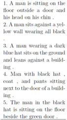
Formal analysis, S.S.R.; Investigation, S.S.R.; Methodology, S.S.R.; Project administration, S.S.R. and S.M.I.; Software, S.S.R.; Supervision, S.M.I.; Validation, S.M.I.; Writing—original draft, S.S.R. and S.M.I.

Funding

The first author of this paper would like to thank University Grants Commission for providing fellowship through UGC NET/JRF scheme.

Conflicts of Interest

The authors declare no conflict of interest.

References

  1. Mikolov, T.; Karafiát, M.; Burget, L.; Černocký, J.; Khudanpur, S. Recurrent neural network based language model. In Proceedings of the Conference of the International Speech Communication Association, Makuhari, Chiba, Japan, 26–30 September 2010; DBLP. pp. 1045–1048. [Google Scholar]
  2. Hochreiter, S.; Schmidhuber, J. Long short-term memory. Neural Comput. 1997, 9, 1735–1780. [Google Scholar] [CrossRef] [PubMed]
  3. Vinyals, O.; Toshev, A.; Bengio, S.; Erhan, D. Show and tell: A neural image caption generator. In Proceedings of the IEEE Conference on Computer Vision and Pattern Recognition, Boston, MA, USA, 7–12 June 2015. [Google Scholar]
  4. Karpathy, A.; Joulin, A.; Fei-Fei, L. Deep Fragment Embeddings for Bidirectional Image Sentence Mapping. Adv. Neural Inf. Process. Syst. 2014, arXiv:1406.5679. [Google Scholar]
  5. Bernardi, R.; Cakici, R.; Elliott, D.; Erdem, A.; Erdem, E.; Ikizler-Cinbis, N.; Keller, F.; Muscat, A.; Plank, B. Automatic Description Generation from Images: A Survey of Models, Datasets, and Evaluation Measures. J. Artif. Intell. Res. (JAIR) 2016, 55, 409–442. [Google Scholar] [CrossRef]
  6. Mitchell, M.; Dodge, J.; Goyal, A.; Yamaguchi, K.; Stratos, K.; Mensch, A.; Berg, A.; Han, X.; Berg, T.; Health, O. Midge: Generating Image Descriptions From Computer Vision Detections. In Proceedings of the 13th Conference of the European Chapter of the Association for Computational Linguistics, Avignon, France, 23–27 April 2012; pp. 747–756. [Google Scholar]
  7. Kulkarni, G.; Premraj, V.; Ordonez, V.; Dhar, S.; Li, S.; Choi, Y.; Berg, A.C.; Berg, T.L. Baby talk: Understanding and generating simple image descriptions. IEEE Trans. Pattern Anal. Mach. Intell. 2013, 35, 2891–2903. [Google Scholar] [CrossRef] [PubMed]
  8. Ordonez, V.; Kulkarni, G.; Berg, T.L. Im2text: Describing images using 1 million captioned photographs. Adv. Neural Inf. 2011, 1143–1151. [Google Scholar]
  9. Hodosh, M.; Young, P.; Hockenmaier, J. Framing image description as a ranking task: Data, models and evaluation metrics. J. Artif. Intell. Res. 2013, 47, 853–899. [Google Scholar] [CrossRef]
  10. Socher, R.; Karpathy, A.; Le, Q.V.; Manning, C.D.; Ng, A.Y. Grounded Compositional Semantics for Finding and Describing Images with Sentences. Trans. Assoc. Comput. Linguist. 2014, 2, 207–218. [Google Scholar] [CrossRef]
  11. Lu, J.; Xiong, C.; Parikh, D.; Socher, R. Knowing when to look: Adaptive attention via a visual sentinel for image captioning. In Proceedings of the IEEE Conference on Computer Vision and Pattern Recognition (CVPR), Honolulu, HI, USA, 21–26 July 2017; Volume 6. [Google Scholar]
  12. Farhadi, A.; Hejrati, M.; Sadeghi, M.A.; Young, P.; Rashtchian, C.; Hockenmaier, J.; Forsyth, D. Every picture tells a story: Generating sentences from images. In Lecture Notes in Computer Science (Including Subseries Lecture Notes in Artificial Intelligence and Lecture Notes in Bioinformatics); 6314 LNCS (PART 4); Springer: Berlin/Heidelberg, Geramny, 2010; pp. 15–29. [Google Scholar]
  13. Kiros, R.; Salakhutdinov, R.; Zemel, R. Multimodal neural language models. In Proceedings of the 31st International Conference on Machine Learning (ICML-14), Beijing, China, 21–26 June 2014. [Google Scholar]
  14. Gong, Y.; Wang, L.; Hodosh, M.; Hockenmaier, J.; Lazebnik, S. Improving image-sentence embeddings using large weakly annotated photo collections. In European Conference on Computer Vision; Springer: Cham, Switzerland, 2014. [Google Scholar]
  15. Karpathy, A.; Li, F.-F. Deep visual-semantic alignments for generating image descriptions. In Proceedings of the IEEE Conference on Computer Vision and Pattern Recognition, Boston, MA, USA, 7–12 June 2015. [Google Scholar]
  16. Donnelly, C. Image Caption Generation with Recursive Neural Networks; Department of Electrical Engineering, Stanford University: Palo Alto, CA, USA, 2016. [Google Scholar]
  17. Soh, M. Learning CNN-LSTM Architectures for Image Caption Generation; Dept. Comput. Sci., Stanford Univ.: Stanford, CA, USA, 2016. [Google Scholar]
  18. Wang, C.; Yang, H.; Bartz, C.; Meinel, C. Image captioning with deep bidirectional LSTMs. In Proceedings of the 2016 ACM on Multimedia Conference, New York, NY, USA, 6–9 June 2016. [Google Scholar]
  19. You, Q.; Jin, H.; Wang, Z.; Fang, C.; Luo, J. Image captioning with semantic attention. In Proceedings of the IEEE Conference on Computer Vision and Pattern Recognition, Las Vegas, NV, USA, 26 June–1 July 2016. [Google Scholar]
  20. Anderson, P.; He, X.; Buehler, C.; Teney, D.; Johnson, M.; Gould, S.; Zhang, L. Bottom-up and top-down attention for image captioning and visual question answering. In Proceedings of the IEEE Conference on Computer Vision and Pattern Recognition, Salt Lake City, UT, USA, 18–22 June 2018. [Google Scholar]
  21. Poghosyan, A.; Sarukhanyan, H. Short-term memory with read-only unit in neural image caption generator. In Proceedings of the 2017 Computer Science and Information Technologies (CSIT), Yerevan, Armenia, 25–29 September 2017. [Google Scholar]
  22. Aneja, J.; Deshpande, A.; Schwing, A.G. Convolutional image captioning. In Proceedings of the IEEE Conference on Computer Vision and Pattern Recognition, Salt Lake City, UT, USA, 18–22 June 2018. [Google Scholar]
  23. Chen, F.; Ji, R.; Sun, X.; Wu, Y.; Su, J. Groupcap: Group-based image captioning with structured relevance and diversity constraints. In Proceedings of the IEEE Conference on Computer Vision and Pattern Recognition, Salt Lake City, UT, USA, 18–22 June 2018. [Google Scholar]
  24. Tan, Y.H.; Chan, C.S. phi-LSTM: A Phrase-Based Hierarchical LSTM Model for Image Captioning; Springer International Publishing: Cham, Switzerland, 2017; pp. 101–117. [Google Scholar]
  25. Han, M.; Chen, W.; Moges, A.D. Fast image captioning using LSTM. Cluster Comput. 2019, 22, 6143–6155. [Google Scholar] [CrossRef]
  26. He, C.; Hu, H. Image captioning with text-based visual attention. Neural Process. Lett. 2019, 49, 177–185. [Google Scholar] [CrossRef]
  27. Zeiler, M.D.; Rob, F. Visualizing and understanding convolutional networks. In European Conference on Computer Vision; Springer International Publishing: Berlin, Germany, 2014. [Google Scholar]
  28. LeCun, Y.; Bottou, L.; Bengio, Y.; Haffner, P. Gradient-based learning applied to document recognition. Proc. IEEE 1998, 86, 2278–2324. [Google Scholar] [CrossRef]
  29. Krizhevsky, A.; Sutskever, I.; Hinton, G. ImageNet Classification with Deep Convolutional Neural Networks. In Proceedings of the NIPS, Lake Tahoe, NV, USA, 3–8 December 2012. [Google Scholar]
  30. Simonyan, K.; Zisserman, A. Very Deep Convolutional Networks for Large-Scale Image Recognition. In Proceedings of the ICLR, San Diego, CA, USA, 7–9 May 2015. [Google Scholar]
  31. Szegedy, C.; Liu, W.; Jia, Y.; Sermanet, P.; Reed, S.; Anguelov, D.; Erhan, D.; Vanhoucke, V.; Rabinovich, A. Going deeper with convolutions. In Proceedings of the CVPR, Las Vegas, NV, USA, 7–13 December 2015. [Google Scholar]
  32. He, K.; Zhang, X.; Ren, S.; Sun, J. Deep residual learning for image recognition. In Proceedings of the IEEE Conference on Computer Vision and Pattern Recognition, Portland, OR, USA, 23–28 June 2014. [Google Scholar]
  33. Srivastava, R.K.; Greff, K.; Schmidhuber, J. Highway networks. arXiv 2015, arXiv:1505.00387. [Google Scholar]
  34. Huang, G.; Liu, Z.; Van Der Maaten, L.; Weinberger, K.Q. Densely connected convolutional networks. arXiv 2016, arXiv:1608.06993. [Google Scholar]
  35. Sandler, M.; Howard, A.; Zhu, M.; Zhmoginov, A.; Chen, L.C. Mobilenetv2: Inverted residuals and linear bottlenecks. In Proceedings of the IEEE Conference on Computer Vision and Pattern Recognition, Salt Lake City, UT, USA, 18–22 June 2018. [Google Scholar]
  36. Iandola, F.N.; Han, S.; Moskewicz, M.W.; Ashraf, K.; Dally, W.J.; Keutzer, K. SqueezeNet: AlexNet-level accuracy with 50x fewer parameters and <0.5 MB model size. arXiv 2016, arXiv:1602.07360. [Google Scholar]
  37. Mikolov, T.; Chen, K.; Corrado, G.; Dean, J. Efficient estimation of word representations in vector space. arXiv 2013, arXiv:1301.3781. [Google Scholar]
  38. Pennington, J.; Socher, R.; Manning, C. Glove: Global vectors for word representation. In Proceedings of the 2014 conference on empirical methods in natural language processing (EMNLP), Doha, Qatar, 25–29 October 2014. [Google Scholar]
  39. Joulin, A.; Grave, E.; Bojanowski, P.; Douze, M.; Jégou, H.; Mikolov, T. Fasttext. zip: Compressing text classification models. arXiv 2016, arXiv:1612.03651. [Google Scholar]
  40. Von Neumann, O. Morgenstern, Theory of Games and Economic Behavior; copyright 1944; Princeton University Press: Princeton, NJ, USA, 1953. [Google Scholar]
  41. Sun, X.; Liu, Y.; Li, J.; Zhu, J.; Liu, X.; Chen, H. Using cooperative game theory to optimize the feature selection problem. Neurocomputing 2012, 97, 86–93. [Google Scholar] [CrossRef]
  42. Papineni, K.; Roukos, S.; Ward, T.; Zhu, W.J. BLEU: A method for automatic evaluation of machine translation. In Proceedings of the 40th annual meeting on association for computational linguistics, Association for Computational Linguistics, Philadelphia, PA, USA, 7–12 July 2002. [Google Scholar]
  43. Xu, K.; Ba, J.; Kiros, R.; Cho, K.; Courville, A.; Salakhudinov, R.; Zemel, R.; Bengio, Y. Show, attend and tell: Neural image caption generation with visual attention. Int. Conf. Mach. Learn. 2015, arXiv:1502.03044. [Google Scholar]
  44. Tan, Y.H.; Chan, C.S. Phrase-based Image Captioning with Hierarchical LSTM Model. arXiv 2017, arXiv:1711.05557. [Google Scholar]
Figure 1. Architecture of the proposed model.
Information 10 00354 g001
Figure 2. Architecture of the image model.
Information 10 00354 g002
Figure 3. Architecture of Densenet.
Information 10 00354 g003
Figure 4. Architecture of the language model.
Information 10 00354 g004
Figure 5. Comparison of the accuracies of different models.
Information 10 00354 g005
Figure 6. Comparison of the losses of different models.
Information 10 00354 g006
Figure 7. Comparison of the BLEU scores under different beam sizes.
Information 10 00354 g007
Table 1. Classification of generated captions based on the Bilingual Evaluation Understudy (BLEU) scores.
BLEU-1BLEU-2BLEU-3BLEU-4Class
>0.8>0.6>0.5>0.4Successful
≤0.7≤0.5≤0.4≤0.3Unsuccessful
OtherwisePartially successful
Table 2. Successful results.
Sl. NoImageGround Truth CaptionsGenerated Caption
1 Information 10 00354 i001 Information 10 00354 i002A man with a stick in its mouth is standing on a snow covered field.
2 Information 10 00354 i003 Information 10 00354 i004A brown dog and a brown dog are running in a grassy field.
3 Information 10 00354 i005 Information 10 00354 i006A man in a blue jacket is sitting on a city street.
Table 3. Partially successful results.
Sl. NoImageGenerated Caption
1 Information 10 00354 i007A group of people in a crowd.
2 Information 10 00354 i008A brown dog with a stick in its mouth.
Table 4. Unsuccessful results.
Sl. NoImageGenerated Caption
1 Information 10 00354 i009A dog with a ball in its mouth.
3 Information 10 00354 i010A man with a stick in its mouth with a stick in its mouth.
Table 5. Classification results.
Total number of images:1000
Number of successful images:558
Success rate:55.8%
Number of partially successful images:412
Partial success rate:41.2%
Number of unsuccessful images:30
Unsuccessful rate:3%
Table 6. Comparison of the BLEU scores for different models. NIC, Neural Image Caption.
ModelBLEU-1BLEU-2BLEU-3BLEU-4
Google NIC (Vinyals et al. 2014) [3]63.041.027.0-
Log bilinear(kiros et al. 2014) [13]65.642.427.717.7
Hard attention [43]67.045.731.421.3
Soft attention [43]6744.829.919.5
Phi-LSTM [24]6744.829.919.5
Phi-LSTMv2 (w.o.r) [44]61.543.129.619.7
Phi-LSTMv2 (w.r) [44]62.749.430.720.8
Our Model (beam search) 67.255.0544.4240.61
Our Model (game theoretic search) 69.9656.346.4542.95

