Article

Studying Transaction Fees in the Bitcoin Blockchain with Probabilistic Logic Programming †

1
Dipartimento di Ingegneria, University of Ferrara, Via Saragat 1, I-44122 Ferrara, Italy
2
Dipartimento di Matematica e Informatica, University of Ferrara, Via Saragat 1, I-44122 Ferrara, Italy
*
Author to whom correspondence should be addressed.
This paper is an extended version of our paper published in BSCT 2019—Azzolini, D.; Riguzzi, F.; Lamma, E. Analyzing Transaction Fees with Probabilistic Logic Programming.
Information 2019, 10(11), 335; https://doi.org/10.3390/info10110335
Submission received: 30 September 2019 / Revised: 25 October 2019 / Accepted: 26 October 2019 / Published: 30 October 2019
(This article belongs to the Special Issue Blockchain and Smart Contract Technologies)

Abstract

:
In Bitcoin, if a miner is able to solve a computationally hard problem called proof of work, it will receive an amount of bitcoin as a reward which is the sum of the fees for the transactions included in a block plus an amount inversely proportional to the number of blocks discovered so far. At the moment of writing, the block reward is several orders of magnitude greater than the sum of transaction fees. Usually, miners try to collect the largest reward by including transactions associated with high fees. The main purpose of transaction fees is to prevent network spamming. However, they are also used to prioritize transactions. In order to use the minimum amount of fees, users usually have to find a compromise between fees and urgency of a transaction. In this paper, we develop a probabilistic logic model to experimentally analyze how fees affect confirmation time and miner’s revenue and to predict if an increase of average fees will generate a situation when the miner gets more reward by not following the protocol.

1. Introduction

Since its first proposal in 2008 by Nakamoto [1], bitcoin and blockchain (even if this second term is not directly used in Nakamoto’s paper) started to attract the interest of many users and researchers. The main feature of a blockchain system is that it allows everyone to exchange cryptocurrencies in a fully decentralized way, without the need of a trusted third party. The features of blockchains have been extended with the creation of blockchain 2.0 systems [2] where users can develop smart contracts, programs allowing interaction in a fully decentralized way.
There are several blockchain systems currently available such as Ethereum [3,4], EOSIO [5], Hyperledger [6], and Cardano [7], but Bitcoin still has the highest market capitalization (https://coinmarketcap.com/).
All blockchain systems are based on a distributed ledger shared among the peers. This ledger allows everyone to check the validity of every single transaction, from the first one to the last issued, and to reconstruct in a fully deterministic way the whole history, thanks to the use of several layers of cryptography.
In order to validate blocks, miners usually follow a consensus protocol. In the case of Bitcoin, this involves the solution of a computationally hard problem called Proof of Work that will allow the solver to append a block to the blockchain. A transaction is a transfer of bitcoin from the issuer to the recipient. In order to prevent spamming in the network, each transaction provides an amount of fees collected by the miner as a reward for his work. However, fees are also a mechanism to prioritize transactions, as miners prefer to include the most profitable transactions in a block, to get the highest possible reward. This situation opens several possible scenarios where miners deviate from the protocol on purpose, in order to get a higher revenue.
Miners are driven by economical incentives. Their profit comes from block reward and transaction fees and so, since block reward is specified in the protocol and decreases at a known rate (every 210,000 blocks), transactions fees will have a central role in the future. Moreover, in order to sustain mining operations, cryptocurrencies at the moment need to have a value also in fiat money.
The size of the blockchain increases over time and so does the cost of the equipment needed to store and manage it. If the value of a cryptocurrency is too low, the work of the miners (as in Bitcoin) will not be profitable and so they will leave the system. An interesting study (https://medium.com/coinmonks/survey-of-eos-block-producers-cf9677561db7) conducted on EOS, eighth for market capitalization (https://coinmarketcap.com/) at the moment of writing, shows that block producers are struggling to break even, due to the low value of the cryptocurrency.
Probabilistic (Logic) Programming [8] (PLP) has been applied to model several domains [9] including the Bitcoin protocol [10] and is a powerful tool for modelling and predicting several situations that can happen in a blockchain environment.
In this paper, we focus on Bitcoin and, starting from several real world-values, such as average block size and average block reward, we model how transaction fees influence a miner’s revenue and the probability of inclusion of a transaction in a block using PLP. The goal of this model is to analyze, from two different points of view, the economic incentives for both miners and users. We then extend this model to a situation where the gap between block reward and transaction fees reduces and a situation where the collected fees are higher than the block reward, to show whether a fork will be profitable for an attacker. With this second model, we analyze the stability of the system when the current main source of mining income (block reward) reduces and transaction fees increase. In this way, the earnings are driven by external factors not defined in the protocol. Users may then drive and influence miners’ profit, thus creating instability and unreliability in the system, a situation that can reduce the number of users and thus the value of bitcoin.
The paper is structured as follows: in Section 2, we give a brief overview of Bitcoin, blockchain ad transaction fees. Section 3 introduces basic knowledge of PLP needed to understand the models. Section 4 shows how we applied PLP to model the blockchain and presents the results. Section 5 discusses related work and Section 6 concludes the paper.

2. Blockchain, Bitcoin, and Fees

Every blockchain system is based on a distributed ledger shared among the users. This ledger is composed by several blocks that are collections of transactions. A strong layer of cryptography is at the basis of the system and allows transactions to be linked together, giving them a temporal order. This idea of secure timestamping goes back to 1991 [11].
One of the most famous blockchains is the Bitcoin blockchain, born in 2008 and now with more than 300 thousand of transactions issued every day (https://www.blockchain.com/it/charts/n-transactions). Every user can download and maintain a copy of the ledger, since the whole blockchain is public. However, the Bitcoin blockchain requires a lot of disk space for storage (https://www.blockchain.com/charts/blocks-size). In order to increase the adoption of the system, Bitcoin provides a lightweight client that can be used by almost every device, as opposed to a full client. The main difference is that lightweight clients track only the owner’s transactions while full clients track all the transactions.
A transaction can be sent from a user to another user and implies a movement of bitcoins from the issuer to the recipient. A transaction is composed by a set of inputs and outputs. Usually, inputs and outputs do not sum up to the same amount. The difference is collected as transaction fees by the miner who includes the transaction into a block in the blockchain.
Users are called peers, and, in this paper, we will often use users and peers interchangeably. Some of them are miners. The goal of a miner is to provide a Proof of Work (PoW, called hashcash in Bitcoin) to be able to append blocks to the blockchain. One of the main features of PoW is that the validity of the solution can be easily checked by anyone in the network. In order to maintain the average number of blocks discovered constant over time (https://btc.com/stats/diff), usually a block every 10 min), the difficulty of PoW increases over time. In order to increase the probability of finding a new block, miners usually group themselves into mining pools. However, this situation increases the centralization of the network and increases the probability of attacks [12] that undermine the security and the reliability of the system.
Due to several factors such as, for example, network delays, two miners can find two different blocks with two (not necessarily) different sets of transactions at the same time. This situation creates a fork, where the chain is split into two. This ambiguity is solved when the next block is found. If a miner follows the protocols, it should append the last mined block to the longest chain. However, there can be several alternative chains that can be symptoms of a double spending attack [10,12,13]. A double spending attack is a situation where a miner wants to spend multiple times a certain amount of bitcoin. This is possible if the attacker can create an alternative chain longer than the honest one. In this case, all the blocks not part of the longest chain will not be considered valid.
When a new block is appended to the blockchain, the miner who found it receives a reward which is the sum of all the fees of the transactions included in the block plus a substantial amount of bitcoin, through a Coinbase transaction. This amount of bitcoin will decrease over time, as the number of discovered blocks increases.
The size of a block is fixed, even if it is a controversial matter (https://en.bitcoin.it/wiki/Block_size_limit_controversy). Due to this limitation, usually peers include the most profitable transactions into a block, to get the most reward. To increase the priority of a transaction, users can attach a high fee to it in order to increase its probability of being included into a block in a short time. This scenario can, however, reduce the number of users, unwilling to pay too high fees for a single transaction. It is particularly important for a user to find a balance between the fee (usually measured in satoshi per byte, a quantity called fee rate or feerate, where 1 satoshi = 10 8 bitcoin) and the priority of a transaction.
Different situations complicate the calculation of the most profitable fee rate, value that influences also the work of the miners because they decide the set of transactions to include in a block. To show why it is a hard task, consider this example. Imagine there are four transactions waiting to be inserted in a block, A with size 150 kb and fee 150, B with size 250 kb and fee 300, C with size 350 kb and fee 450 and D with size 450 kb and fee 600. Those values are greater than the average size of a transaction, but, in this example, they are used only for illustrative purposes. We can compute the fee rate as f e e / s i z e and obtain 1 for A, 1.2 for B, 1.28 for C, and 1.3 for D. In order to get the maximum reward, a miner can sort the transactions in descending order of fee rate, from the most profitable one to the least one. In our example, we get D, C, B, and A. Then, he selects the most profitable ones and includes them in a block. However, in our case, transactions D, C, and B cannot be stored in the same block since their total size 450 + 350 + 250 = 1050 kb is greater than the block limit of 1000 kb (however, thanks to the soft fork called Segregated Witness (https://github.com/bitcoin/bips/blob/master/bip-0141.mediawiki), in a block explorer, such as (blockchain.com), some blocks may appear bigger than 1 Mb). This shows that the miner should solve a knapsack problem to find the best set of transaction to include in a block.
Consider now a situation where there are dependent transactions. For instance, suppose that C depends from A, i.e., it spends an output of A. In this case, in order to get the reward from C, the miner should include both A and C into the block, even if A has the lowest fee rate of the whole pool. This is a scenario called Child Pay for Parent (https://en.bitcoin.it/wiki/Miner_fees), where a transaction child (C) with a higher fee rate helps the transaction parent (A) with a lower fee rate, by spending one of its output.
Another situation that complicates the estimation of the optimal fee rate is the possibility that miners mine empty blocks, to avoid wasting time to control and validate the last received block and to select a set of transactions. A third noticeable situation that complicates the estimation is the possibility to have forks, which requires that all the blocks not part of the longest chain must be mined again. Another problem is the fact that several variables that condition this calculation are difficult to predict, such as the number of transactions received by the network in a certain time span or block discovery time.
There exist several applications that try to compute the optimal fee rate. One of them is available in Bitcoin (https://bitcoin.org/en/download, one of the most used Bitcoin clients) and is accessible through the command estimatesmartfee. The output of the command is the optimal fee rate to attach to a transaction in order to have it confirmed with high probability in N blocks, where N is selected by the user and can be up to 1008 (at the moment of writing). The algorithm (https://github.com/bitcoin/bitcoin/blob/master/src/policy/fees.h) works as follows: transactions are grouped into exponentially spaced buckets, since tracking every transaction is too expensive both computationally and in terms of memory. Each bucket contains transactions with a similar fee rate. The lowest bucket goes from 1000 satoshis per byte to 1050. The next one goes from 1050 to 1102.5, and so on, up to 10 7 . Each bucket boundary is 1.05 times the previous one. The program then tracks the number of transactions that enter in each bucket and the number of transactions included into a block within the target. The computation is further refined and gives more importance to recent blocks than to older ones.

3. Probabilistic Logic Programming

A wide variety of domains [14,15,16] can be represented using Probabilistic Logic Programming (PLP) languages under the distribution semantics [17,18]. A program in a language adopting the distribution semantics defines a probability distribution over normal logic programs called instances or worlds. Each normal program is assumed to have a total well-founded model [19]. In order to obtain the probability of a query, its distribution is extended to a joint distribution of the query and the worlds. Then, the probability of the query is computed by summing out the world in a process called marginalization. A PLP language under the distribution semantics with a general syntax is that of Logic Programs with Annotated Disjunctions (LPADs) [20]. In the following part, we present the semantics of LPADs for the case of no function symbols, if function symbols are allowed, see [21].
Every logic program is represented by a set of clauses. Each clause is composed by a head and a body. An example of clause is grow(Plant) :- feed(Plant), where grow(Plant) is the head and feed(Plant) is the body. The previous clause can be interpreted as: “if we feed a Plant, it will grow”. Heads of clauses in LPADs are disjunctions in which each atom is annotated with a probability, i.e., a value between 0 and 1. Consider a LPAD T with n clauses: T = { C 1 , , C n } . Each clause C takes the form: h 1 : Π 1 ; ; h v : Π v : b 1 , , b u , where h 1 , , h v are logical atoms, b 1 , , b u are logical literals, and Π 1 , , Π v are real numbers in the interval [ 0 , 1 ] that sum to 1. b 1 , , b u is indicated with b o d y ( C ) . Note that, if v = 1 , the clause corresponds to a non-disjunctive clause. We also allow clauses where k = 1 v Π k < 1 : in this case, the head of the annotated disjunctive clause implicitly contains an extra atom n u l l that does not appear in the body of any clause and whose annotation is 1 k = 1 v Π k .
We define a substitution θ as a function mapping variables to terms. Usually, θ has the form θ = { X 1 / t 1 , ... , X k / t k } meaning that each variable X i is replaced by term t i . Applying a substitution θ to an LPAD T means replacing all the occurrences of each variable X j in T by the corresponding term t j . We denote by g r o u n d ( T ) the grounding of an LPAD T, i.e., the replacement of all the variables in the program with constants in all possible ways. Clauses without variable are called ground.
Each grounding C i θ j of a clause C i corresponds to a random variable X i j with values { 1 , , v i } , where v i is the number of head atoms of C i . The random variables X i j are independent of each other. An atomic choice [22] is a triple ( C i , θ j , k ) where C i T , θ j is a substitution that grounds C i and k { 1 , , v i } identifies one of the head atoms. In practice, ( C i , θ j , k ) corresponds to an assignment X i j = k .
A selection σ is a set of atomic choices that contains an atomic choice ( C i , θ j , k ) for each clause C i θ j in g r o u n d ( T ) . A selection σ identifies a normal logic program l σ defined as l σ = { ( h i k : b o d y ( C i ) ) θ j | ( C i , θ j , k ) σ } . l σ is called an instance, possible world, or simply world of T. Since the random variables associated with ground clauses are independent, we can assign a probability to instances P ( l σ ) = ( C i , θ j , k ) σ Π i k .
We consider only sound LPADs, where, for each selection, the well-founded model [18] of the program l σ chosen by σ is two-valued, i.e., each ground atom is either true or false. We write l σ q to mean that the query q (a ground atom) is true in the well-founded model of the program l σ . Since the well-founded model of each world is two-valued, q can only be true or false in l σ .
We denote the set of all instances by L T . Let P ( L T ) be the distribution over instances. The probability of a query q (a ground atom) given an instance l is P ( q | l ) = 1 if l q and 0, otherwise. The probability of q is given by
P ( q ) = l L T P ( q , l ) = l L T P ( q | l ) P ( l ) = l L T : l q P ( l ) .
An example of LPAD is:
e a r t h q u a k e ( X , s t r o n g ) : 0.3 ; e a r t h q u a k e ( X , m o d e r a t e ) : 0.5 : f a u l t _ r u p t u r e ( X ) , e a r t h q u a k e ( X , s t r o n g ) : 0.2 ; e a r t h q u a k e ( X , m o d e r a t e ) : 0.6 : v o l c a n i c _ e r u p t i o n ( X ) , f a u l t _ r u p t u r e ( s t r o m b o l i ) , v o l c a n i c _ e r u p t i o n ( s t r o m b o l i ) , v o l c a n i c _ e r u p t i o n ( v e s u v i o ) .
The program models the occurrence of an earthquake depending on its possible causes. It can be interpreted as: if an earthquake at a site X is caused only by the rupture of a geological fault, we have a strong earthquake with probability 0.3, a moderate earthquake with probability 0.5 and no earthquake with probability 0.2. Note that the probability of not having an earthquake is not explicitly written but is computed as 1 0.3 0.5 = 0.2 . The second clause can be read as—if an earthquake at a site X is caused only by a volcanic eruption, we have a strong earthquake with probability 0.2, a moderate earthquake with probability 0.6, and no earthquake with probability 0.2. The last three facts state that there is a fault rupture at stromboli, there is a volcanic eruption at stromboli, and there is a volcanic eruption at vesuvio, all three with certainty. We can now ask what the probability of a strong earthquake is at stromboli using cplint [15,16].
Probabilistic Logic Programs can include also continuous variables. In this case, those programs are called hybrid. In cplint, users can specify a probability density of a variable V a r of an atom a using the following syntax: a : D e n s i t y B o d y , where D e n s i t y is an atom identifying a probability density and B o d y is the regular body of clause (optional). For example, b(X):beta(X,2,5) states that the variable X follows a Beta distribution with parameters α = 2 and β = 5 .
Given an LPAD, the main task is to perform inference. There are two types of inferences: exact inference and approximate inference. Both approximate and exact inference are implemented into cplint [15,16]. Exact inference tries to compute the exact probability of a query [23]. However, this task is not always feasible because of the #P-completeness [24] of the problem. Alternatively, we can use approximate inference that solves the task providing approximate results.

Approximate Inference and Conditional Approximate Inference

To perform approximate inference, cplint uses Monte Carlo algorithms [25,26]. The general steps of a Monte Carlo algorithm are the following:
  • Sample a head for each ground clause to sample a world,
  • Check if the query is true in the world,
  • Compute the probability of the query as the fraction of samples where the query is true,
  • Repeat the three previous steps until convergence or for a fixed number of steps.
The accuracy of these algorithms depends on the number of iterations. In some cases, where the domain of a program is very large, approximate inference may still require some time due to the necessity of sampling many random variables to generate a world. In this case, to decrease the complexity of the computation, samples can be evaluated lazily, i.e., only when the sampling of a probabilistic clause is required [18].
With Monte Carlo methods, we can also compute the probability of a query q given evidence e. This measure is called conditional probability and is usually indicated with P ( q e ) . Some of the most famous algorithms that perform conditional inference are the so-called Markov Chain Monte Carlo algorithms such as Metropolis–Hastings [16,27]. In this paper, we consider conditional probability queries where the evidence is on atoms that have discrete values. In case of evidence on continuous values, likelihood weighting should be used [28], which computes the probability of the query by summing all the weights of every sample where the query is true and then dividing this value by the total sum of the weights of the samples. Conditional approximate inference can be performed in cplint using the MCINTYRE [25] module.
The following example shows how to represent a mixture of two Gaussians:
h e a d s : 0.7 ; t a i l s : 0.3 , g ( X ) : g a u s s i a n ( X , 0 , 2 ) , h ( X ) : g a u s s i a n ( X , 4 , 1 ) , m i x ( X ) : t a i l s , g ( X ) , m i x ( X ) : h e a d s , h ( X ) .
The logic is the following: we toss a biased coin that has probability 0.7 of landing heads and 0.3 to land tails. If it lands tails, X in mix(X) is sampled from a Gaussian distribution with mean 0 and variance 2, while, if it lands tails, X is still sampled from a Gaussian distribution, but, in this case, the mean is 4, and the variance is 1.
Using cplint, we can take N samples of X in m i x ( X ) by querying mc_sample_arg (mix(X),N,X,L0) or we can take N samples of X in m i x ( X ) given that h e a d s was true by querying mc_mh_sample_arg(mix(X),heads,N,X,L0).
When the values of a random variable are numeric, we can compute its expected value (also called expectation), which is the average of the values obtained by repeating infinitely often the experiment it represents [18]. For a discrete variable X, its expectation is E ( X ) = x x P ( x ) , while, for a continuous variable, is E ( X ) = x P ( x ) d x . In cplint, we can compute the expectation of a random variable using the predicate mc_expectation/4.

4. Modelling Transaction Fee with Probabilistic Logic Programming

One of the most discussed topics in Bitcoin is transaction fees. As mentioned in the previous sections, miners want to maximize their profit by including only the most profitable transactions in a block, while users want to minimize the fees they have to pay for a transaction. An exact formula to compute the optimal value for both miners and users is difficult to obtain due to several variables being difficult to predict.
Block discovery time [29] is the time required to discover a new block. It can be represented with a Poisson distribution with rate (a parameter indicated with λ ) 10. The Poisson distribution is a discrete probability distribution over the number of events occurring in a fixed interval of time. One of the key requisites is that the events are independent and they occur at a known constant rate. In the case of block discovery, the average discovery time is 10 min and this value is kept almost fixed thanks to an update of the difficulty of PoW every 2016 blocks (through a modification of the target value). Moreover, the discovery of each block can be thought as independent.
The computation is further complicated due to several other variables such as the size of a transaction, the size of a block, and the number of transactions broadcast every second. We modeled the first two variables using Normal distributions, characterized by two parameters known as mean ( μ ) and variance ( σ 2 ) and often used to model data distributed around a certain value, and the number of transaction broadcast every second with a Poisson distribution. A Normal distribution is a continuous probability distribution while the size of a transaction is a discrete variable that would be better modeled with a discrete distribution such as the Poisson. However, thanks to the central limit theorem, the Poisson distribution with mean λ can be approximated with a Gaussian distribution with mean and variance λ , i.e., P o i s s o n ( λ ) G a u s s i a n ( λ , λ ) . The average size of a transaction and the average number of transactions added to the mempool per second are retrieved from the website blockchain.com (https://www.blockchain.com/en/charts).
Other variables can affect the block production process. For instance, due to network delays, the mempool (i.e., the set of unconfirmed transactions) can be different from miner to miner. Moreover, the network latency can also be responsible for forks. For instance, when two blocks (let’s call them A and B) are discovered approximately at the same time, some peers can receive A and then B while others can receive them in the opposite order. Consequently, a group of peers will try to extend the chain building upon A and other buildings upon B. However, we will not consider these two cases in our simulation.
We now propose a model to compute the amount of fees collected by a miner over time (Section 4.1). Then, we extend the previous model (Section 4.2) to compute whether a fork will be profitable for an attacker when the gap between transaction fees and Coinbase reduces.
In these models, we make the following assumptions:
  • The total mining (hashing) power in the network is constant. The attacker has a fraction β of the total power (hence, the rest of the network has 1- β )
  • All miners except for the attacker are honest (i.e., they mine on the main chain)

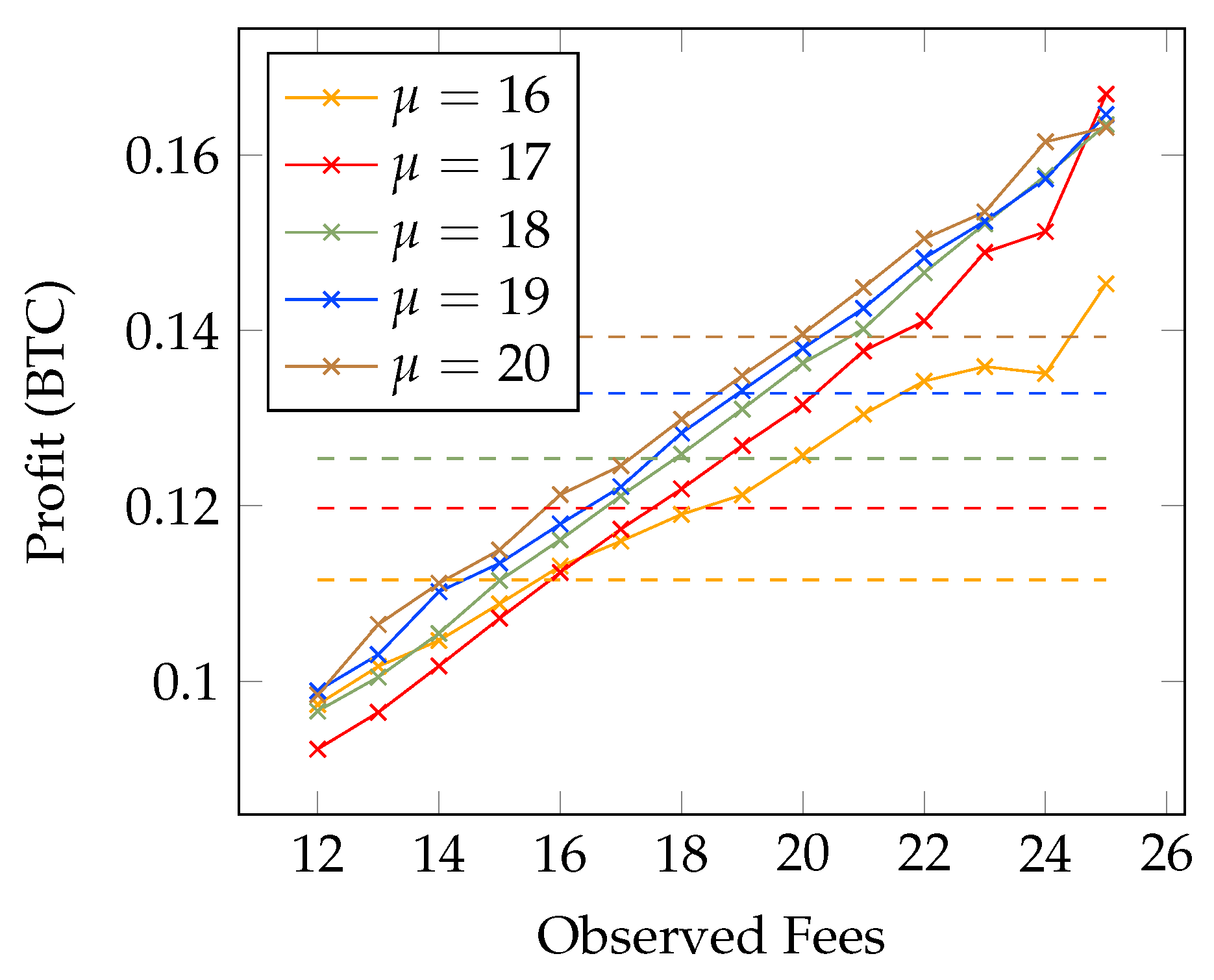
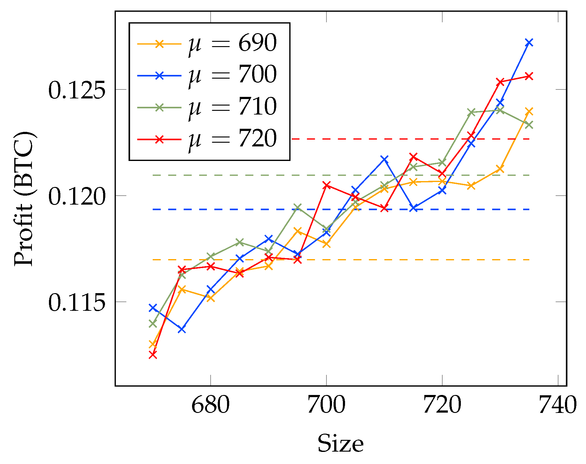
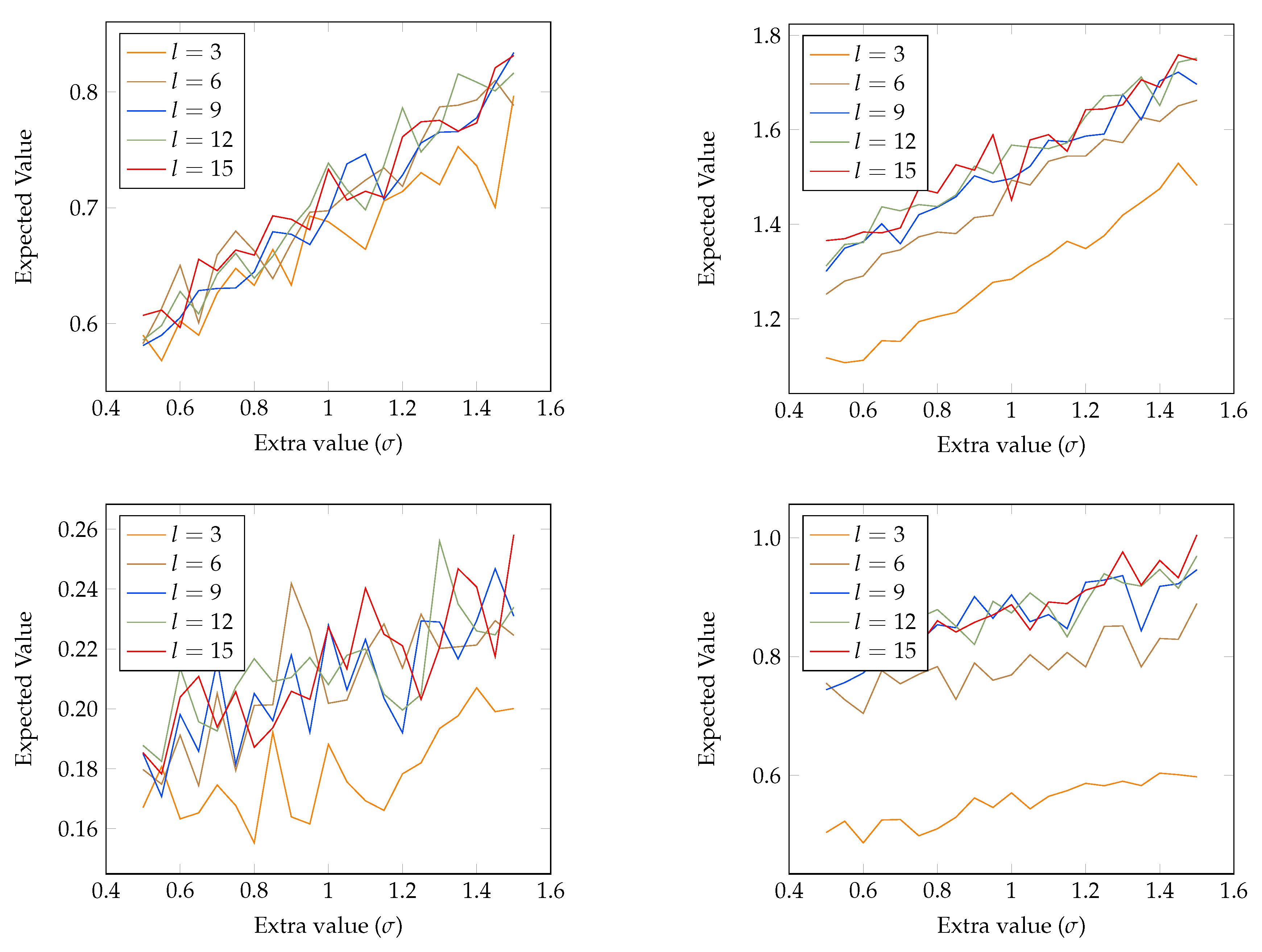
4.1. Analyzing Transaction Fees

The goal of the first model is to compute how transaction fees affect the average profit of a miner. At the moment of writing, the reward of a miner is composed by the sum of the block reward and the sum of all the fees of the transactions contained in the block. Currently, the block reward is 12.5 bitcoin and it is the main source of profit. However, the mining reward halves every 210,000 blocks so, as the chain gets longer, the miner’s profit reduces. In the future, it is possible that the gap between block reward and fees reduces, and thus fees will gain a more important role. This scenario will be analyzed in the next subsection.
In this model, we considered both the block size B and transactions reward R as variables. Both of them are modeled with Gaussian distributions. To make the results more accurate, for both distributions, we sampled the mean from another Gaussian distribution, realizing a Gaussian Mixture Model. Finally, the amount of fees is computed as B R . In this model, we suppose an average block size of 700 kb with variance 25, and we retrieved the average transaction reward from the website blockchain.com. The model is shown in Listing 1.
Listing 1: Model of block fee using Gaussian distributions.
mean_r(M_r):gaussian(M_r,18,2).
mean_b(M):gaussian(M,700,25).
revenue(_,M,R):gaussian(R,M,2).
block_size(_,M,S):gaussian(S,M,25).
val_r(I,V_r):- mean_r(M), revenue(I,M,V).
val_b(I,V_b):- mean_b(M), block_size(I,M,V).
 
obtained_fees(I,O):- val_r(I,R), val_b(I,B), O is R∗B/100000.
The code works as follows: the predicates val_b/2 and val_r/2 compute the size of a block and the fee rate used in obtained_fees/2 to get the amount of fees received for a block creation (the value is divided by 10 5 , since the average fee rate is in satoshi/byte and the block size in kilobyte and we want the output in bitcoin).
Figure 1 shows the expected profit of the miner as a function of the average of the reward M_r and the expected profit of the miner given that we observed V_r in val_r(0,V_r) for different values of V_r. We use the predicates mc_expectation/4 and mc_lw_expectation/5 from the cplint package. The signature of the first predicate is the following: mc_expectation(+Query:atom,+N:int,?Arg:var,-Exp:float). It takes N samples of Query and sums up the value of Arg for each sample. The overall sum is divided by N to give Exp. The second predicate has one more argument, the evidence. The difference with respect to the first one is that each sample is weighted by the likelihood of evidence in the sample, according to likelihood weighting. Figure 2 shows the expected profit of the miner as a function of the average of the block size M_b and the expected profit of the miner given that we observed V_b in val_b(0,V_b) for different values of V_b. For both experiments, we used 1000 samples.
In the second model, we study the variation of the transaction fees over time. In particular, we want to know what the probability is that a transaction with a certain fee rate is confirmed within a number of blocks. This is a useful information for a user’s perspective, given that he usually wants to minimize the fees associated with a transaction. The involved variables are: the average number of transactions in a block, the average block discovery time, and the average number of transactions added to the mempool per second. These variables follow Poisson distributions, but, as explained in the previous section, we approximate them with Gaussian distributions. As before, mean values are obtained from blockchain.com. For the average transaction fee rate, at each iteration, we re-sample the mean of the Gaussian distribution because this value often varies quickly over time. The model can be found in Listing 2.
We first create an initial pool of N transactions by sampling N times the transaction fee from a Gaussian distribution using generate_pool/3 and fee/2. Then, we sort the pool, compute the average number N B of transactions in a block, the average block discovery time T i m e , and the average number of transactions per second T x s (predicates loop_pool/4 and loop_pool_check/4) to compute how many blocks are needed to confirm a transaction with fee rate F. We then compute the number of transactions arrived during the last block creation as T x s T i m e = N N e w T x s . To simulate the inclusion of N N e w T x s transactions in a block, we removed the best N B transactions from the mempool (we suppose the miner acts as expected, i.e., he includes only the most profitable transactions). If the transaction with the best fee rate in the remaining mempool has a value less than F, this means that the transaction we consider has been successfully included in a block and the iteration stops. Otherwise, we simulate the arrival of N N e w T x s new transactions to the mempool with generate_pool/3 and repeat the process.
Listing 2: Model of a pool. The program simulates the arrival of transaction according to a Poisson distribution and the removal of transactions depending on number of transactions in a block and block dicovery time.
average_fee(_,M):uniform(M,15,25).
compute_fee(_,M,F):gaussian(F,M,4).
fee(I,F):- average_fee(I,M), compute_fee(I,M,F).
compute_time(F,M,V):gaussian(F,M,V).
number_of_tx_in_block(_,NB):gaussian(NB,1600,1600).
block_discovery_time(_,Time):gaussian(Time,500,500).
tx_per_second(_,Txs):poisson(Txs,5).
 
generate_pool(N,N,[]):-!.
generate_pool(I,N,[F|T]):- I < N, fee(I,F), I1 is I+1,
    generate_pool(I1,N,T).
get_len(A,B,B):- A >= B, !.
get_len(A,B,A1):- A < B, A1 is A-1.
 
loop_pool(FeeRate,I,NBlocks,Pool):- I =< NBlocks,!,
    number_of_tx_in_block(I,NB), N11 is round(NB),
    length(Pool,LP), get_len(LP,N11,N1),
    length(L,N1), append(L,RemPool,Pool),
    loop_pool_check(FeeRate,I,RemPool,NBlocks).
loop_pool_check(_,_,[],_):- !.
loop_pool_check(FeeRate,_,[H|_],_):- H < FeeRate,!.
loop_pool_check(FeeRate,I,RemPool,NBlocks):- !, I1 is I+1,
    block_discovery_time(I,Time), tx_per_second(I,Txs),
    NNewTxs is Txs∗Time, NT1 is round(NNewTxs),
    generate_pool(0,NT1,NewArrived),
    append(NewArrived,RemPool,NewPool),
    sort(0, @>=, NewPool, PoolSorted),
    loop_pool(FeeRate,I1,NBlocks,PoolSorted).
 
included(_I,FeeRate,NBlocks):-
    loop_pool_check(FeeRate,0,[FeeRate],NBlocks).
 
In this case, we compute the results using both mc_sample/3 and mc_lw_sample/4 provided by the cplint package. The first one samples the goal a certain number of times and computes the probability of success. The second one works in a similar way, but, in addition, performs likelihood weighting: each sample is weighted by the likelihood of the evidence in the sample. For instance, a call to ?- mc_sample(included(1,17,I),5,P1) will sample five times included/3 and return the probability in P1. Similarly, ?- mc_lw_sample(included(1,17,I),fee(0,18),5,P2) samples five times included/3 given that fee(0,18) has been observed and returns the probability in P2. Results are shown in Figure 3. The parameters used are shown in Listing 2. N B l o c k s was set to 1 (next block). ϕ represents the fees associated with a transaction. For instance, if ϕ = 16 , the query is: ?- mc_lw_sample(included(1,16,1),included(0,ObservedFees,1),NSamples,Probability) with ObservedFees ranging between 17 to 23 as in Figure 3. As expected, the confirmation probability decreases as the observed fees increase because, if the fees related to newer blocks increase, a transaction with lower fees will be less likely to be included in a block in a short time. The experiments were executed computing 250 samples. Values of observed fees less than ϕ give probability = 1 because, if the fees related to transactions included in a block are lower than the fees attached to the transaction we are observing, this transaction will be included in the next block, since it is one of the most profitable. For this reason, those values are not reported in the graph.

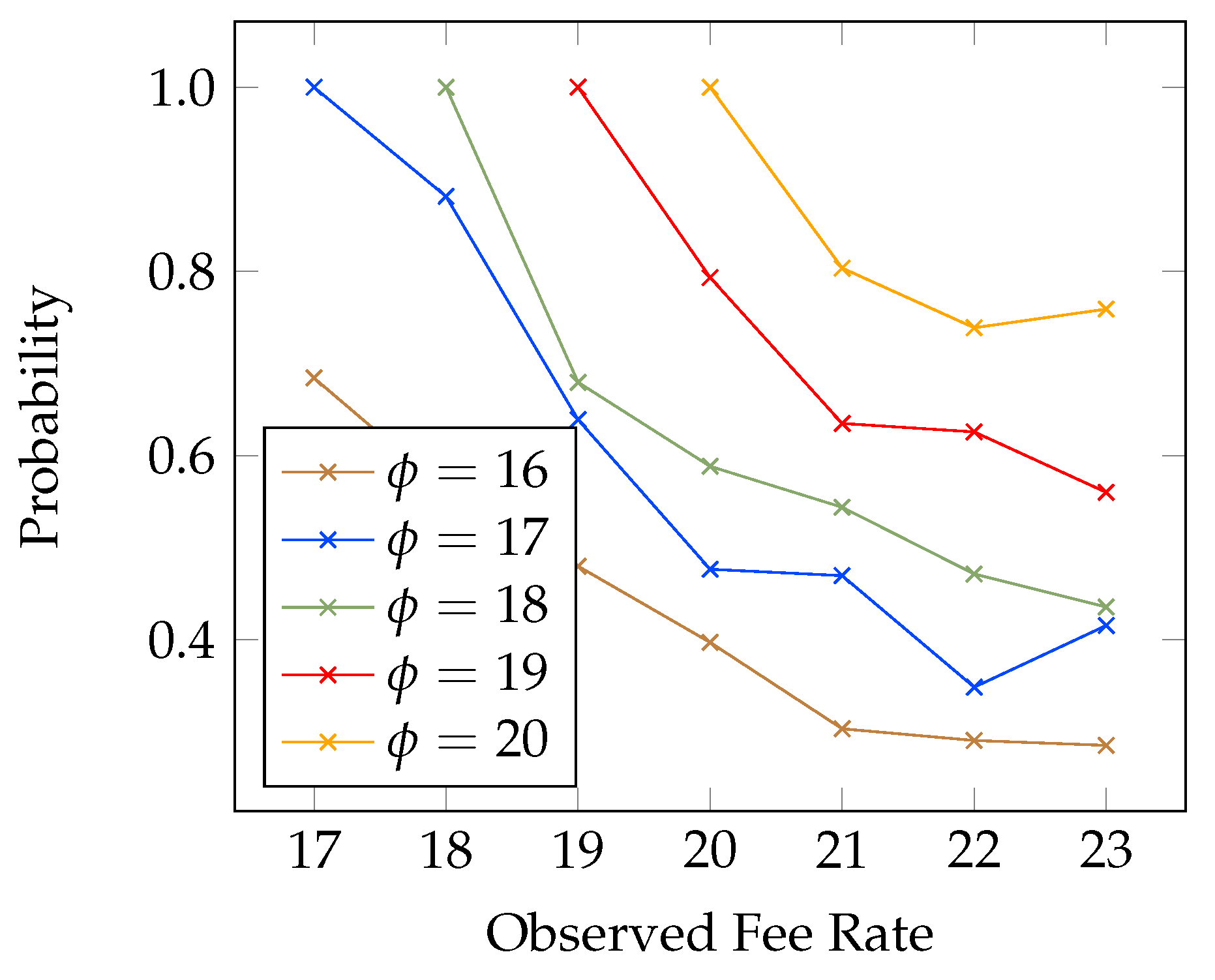
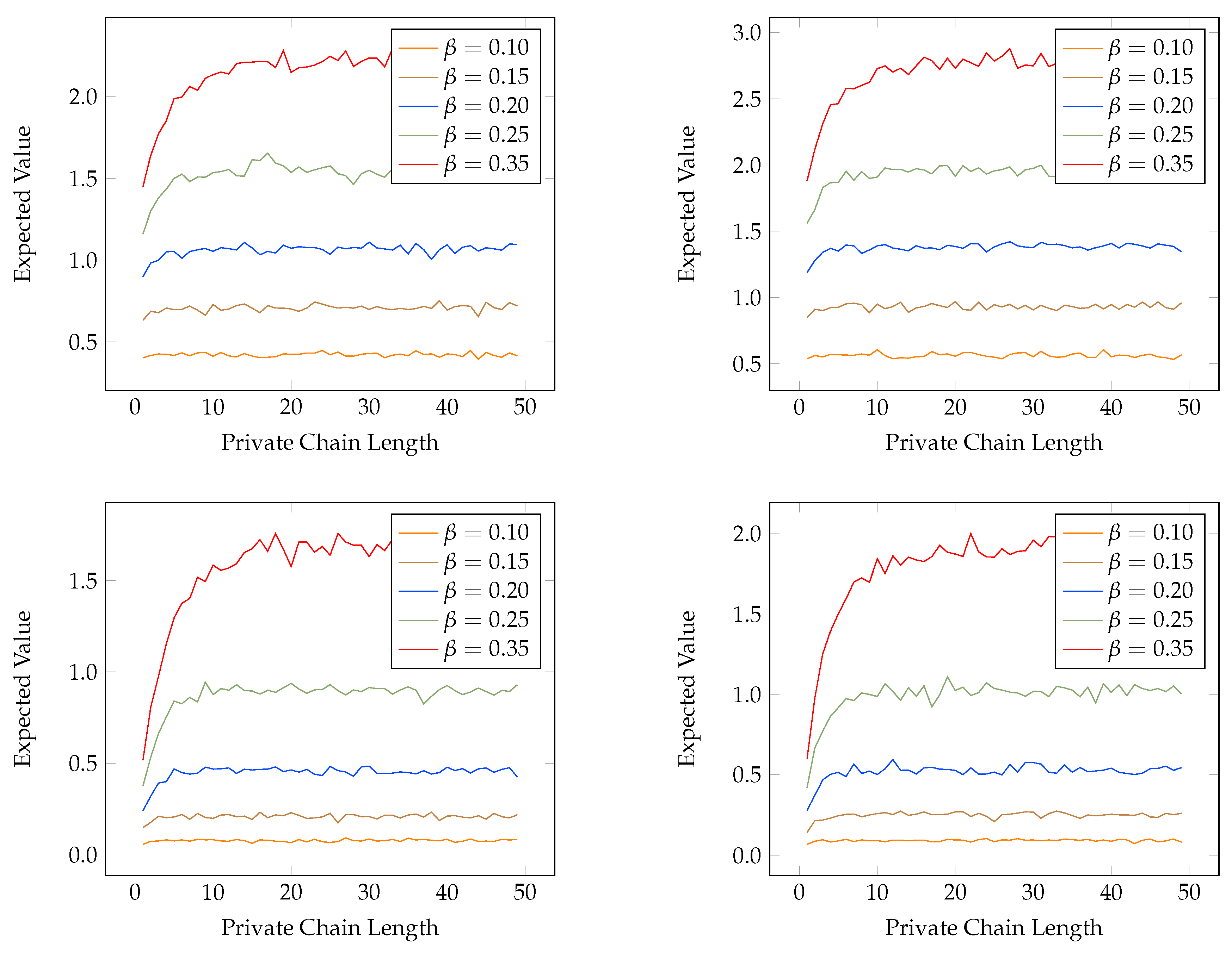
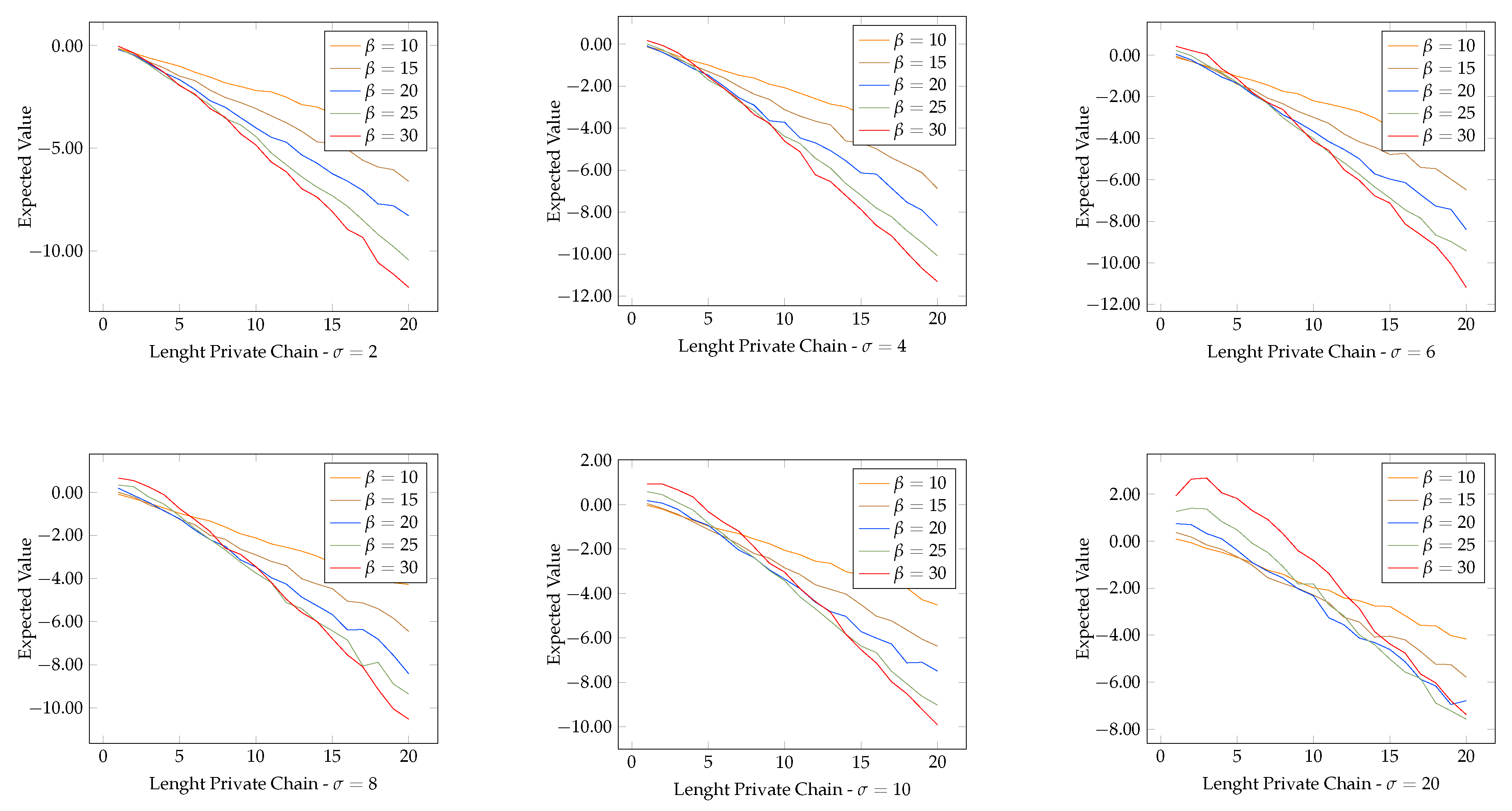
4.2. Probability of Profitable Forks

At the time of writing, the difference between transaction fees and rewards obtained through a Coinbase transaction is still significant. However, in the next few years, the block reward will decrease and, if the system gets more and more users, the transaction fees will likely increase, in order to confirm transactions in an acceptable time. In this section, we analyze what will happen if the gap between block rewards and transaction fees decreases. The goal of these experiments is to show whether deviating from the main chain in order to mine another block with higher fees is profitable from an attacker’s perspective.
Usually, during the analysis of a double spending attack, the model can be divided into two parts: the first one, where the attacker starts to mine his private chain and the second one where the attacker tries to catch up from several blocks behind [12]. In this situation, we are interested in the second part because the attacker tries to fork the chain z (indicated with Z in Listing 3) blocks behind. In our experiments, the initial value of z is set to 1, i.e., the attacker’s fork starts from the second to last block.
This scenario can be represented with a one-dimensional random walk where a particle starts at a position X > 0 and, at each time step, it can move left ( 1 ) or right ( + 1 ) with different probability. Suppose that the miner wants to revert the last block, so the current difference between the length of his private chain and the honest chain is z = 1 . From this starting point, z can increase by one with probability 1 β (a block is added to the main chain) or decrease by 1 with probability β (the attacker found a block and add it to his private chain). This can be represented as:
z t + 1 = z t + 1 , with probability 1 β , z t 1 , with probability β .
The goal of the attacker is to generate a chain longer than the honest one. Once he generates a longer chain, he will publish it, making his fork the longest one so all the transactions not included in the attacker’s chain are not considered valid. Note that, if the attacker controls more than 50% of the total hashing power, he will always succeed in the attack. It is not sure that the walk terminates and so, in order to avoid infinite loops in the program, we limit the difference between the attacker’s chain and the honest chain to 100, i.e., if z > 100 , then the attack fails. In the experiments, we increase the base value of average fee by a factor of 10 (by dividing the output of obtained_fees/2 shown in Listing 1 by 10 4 instead of 10 5 ). In this section, we extend the model presented in [10] where the authors analyze the probability of a successful double spending attack using PLP, without focusing on the economical part of it and without considering transaction fees.
The model used for Figure 4, Figure 5 and Figure 6 can be found in Listing 3. In it, reward_fork/4 is the predicate used to compute the reward. First, it calls obtained_fees/2 described above to get a sample of the obtained fees; then, it calls walk/5, which simulates a one-dimensional, random walk and wraps walk/7, where we set the maximum distance between the honest chain and the attacker chain to 100. The distance between the attacker chain and honest chain decreases or increases by 1 according to the result of move/3. The distance will increase with probability 1 β (where β is the percentage of hashing power controlled by the attacker, indicated with Beta) and decrease with probability β . The run then continues until we eventually reach a point where the attacker creates a chain longer than the honest one or the gap is too big.
Listing 3: Code used for the experiments in Section 4.2.
move(T,P1,1):1-Beta; move(T,P1,-1):Beta:- Beta is P1/100.
 
walk(Z,S,Percentage,ThresholdMinedBlocks,TotalMinedByAttacker):-
    walk(Z,0,S,Percentage,ThresholdMinedBlocks,0,TotalMinedByAttacker).
 
walk(-1,S,S,_,_,V,V).
walk(Z,T0,S,Percentage,ThresholdMinedBlocks,MinedBlocks,VT):-
Z >= 0,
   MinedBlocks < ThresholdMinedBlocks,
   Z < 100,
  move(T0,Percentage,Move),
   T1 is T0+1,
   Z1 is Z+Move,
   ( Move < 0 ->
       V1 is MinedBlocks + 1;
       V1 = MinedBlocks
   ),
   walk(Z1,T1,S,Percentage,ThresholdMinedBlocks,V1,VT).
 
reward_fork(Percentage,ThresholdMinedBLocks,ValueMultiplier,ExpectedReward):-
    coinbase(C),
    obtained_fees(1,AvgFee),
    ExtraValue is AvgFee∗ValueMultiplier,
    (   walk(1,_,Percentage,ThresholdMinedBLocks,Mined) ->
        obtained_fees(2,Fees),
        ExpectedReward is (C+Fees)∗Mined + ExtraValue;
        ExpectedReward is 0
    ).
 
In the first model (threshold model), we want to compute the expected reward obtained from a fork, the relation with hashing power, and length of the private chain. For all the experiments, the average reward for a block (Coinbase + fees) is normalized to 1 and the extra value of a block is indicated with σ (variable ExtraValue in Listing 3). For instance, if σ = 0.5 , this means that the block from which the fork starts has a reward that is 50% larger than the average reward. Figure 4 shows the results. In particular, the graphs show that, at each percentage of controlled hashing power, there is a point where the expected value settles. The graph shows that miner with high computing power should keep mining the private chain even if z is significant. The results are computed using mc_expectation/4 with 10,000 samples. Moreover, as expected, the greater the power of the attacker, the longer his private chain should be in order to get the maximum available reward. The optimal length of the private chain is unchanged as the extra value σ in a block increases. In addition, the length of the private chain gains importance as the number of blocks to catch up increases.
The second experiment (value experiment) relates the expected value obtained trying to re-mine a block with the extra value σ . The results are shown in Figure 5. The graphs show that, if the miner cancels the attack too early, it may have a lower expected reward. In particular, if the extra value related to a block increases, the gap between the length of chains increases. Values are computed using mc_expectation/4 with 10,000 samples.
In the last experiment, we compute the difference between the expected value gained by being honest and the expected value obtained by creating a fork. The expected mining reward from being honest can be seen as the expected value of a binomial distribution where the probability of success is β and failure 1 β . In particular, we are interested in knowing whether there exists an amount of extra value that makes the fork profitable and whether keeping mining a private chain is profitable when the gap from the honest chain is consistent. The graphs in Figure 6 show that a fork will be profitable only for significant values of extra value σ and mining power β .

5. Related Works

Bitcoin, and blockchains in general, attracted a lot of interest in several research fields [30,31]. There are few works related to transaction fees: in [32,33], the authors utilize queuing theory to analyze the relation between fees and confirmation time. In particular, in [33] the authors show that transactions with small fees require a large confirmation time if the arrival of transaction with fees smaller than a certain threshold increases. Moreover, they show that an increase of the block size will not be effective to reduce the confirmation time.
To avoid price fluctuation, the authors in [34] proposed a new method to compute fees based on generalized second price auctions that will reduce the gain obtained by manipulating the system, even if the number of users increases. A game theory approach to study fees can be found in [35] in which the authors show that the current state of the system incentivizes the formations of large miner coalitions. An analysis on how block reward, transaction fees, and their ratio influence the Bitcoin ecosystem can be found in [36]. In [37], the authors analyze a so-called whale attack where a user issues transactions with large fees. In [38], the authors provided an in-depth analysis of transaction fees looking at historical data. In [10,12,13], the authors analyzed and modeled one of the most famous attacks in the PoW system, the double spending attack and show that it is profitable only for high percentage mining power controlled.
Several papers analyzed the economical influence of bitcoin and cryptocurrencies. A broad review can be found in [39]. In particular, in [40,41], the authors show that bitcoin has high volatility. For this reason, the effective reward of the miners may vary quickly over time and thus they should adapt their mining strategy in order to maximize the profit. The instability of the market price is also highlighted in [42] where the authors state that it is very unlikely that bitcoin will replace currencies provided by central banks. The causes of the volatility, according to the authors, can be found in the lack of flexibility of the supply schedule (new bitcoin are created only if a miner is able to provide a correct proof of work), hard written in the code and modifiable only with a hard fork.
The investments made in mining equipment by miners are also an important factor that must be considered in the profit computation, since these investments must be compensated by mining rewards. In this way, investments in mining equipment can be seen as investments in bitcoin. In [43], the authors analyze bitcoin return value according to different investment horizons and show that short-horizon investments can be profitable. In [44,45], the authors analyze whether there is a relation between the price of bitcoin and the investor’s interest based on Google Trends and Wikipedia data, obtaining a strong correlation between price and number of searches on the internet for both data sources. In this way, miners, by looking at number of research works on the internet, can elaborate several strategies, such as reducing the hashing power when the interests in bitcoin decrease. Moreover, an attacker can also decide whether to keep mining his own fork, and whether it will be profitable or not given the expected reward.

6. Conclusions

In this paper, we used Probabilistic Logic Programming to model transaction fees and a possible future situation where the gap between block reward and fees reduces. In detail, we gather the averages of several variables involved in the process and model them with two different probability distributions. We performed two groups of experiments: the first one focused on computing how transaction fees influence miner’s revenue and the probability of confirmation of a transaction within a certain number of blocks. Then, in the second part, we extended this model to analyze a situation where transaction fees and block rewards are similar and whether or not it is profitable for an attacker to try to fork the main chain in order to re-mine a block with particularly high fees. Both models can be easily extended and adapted to new variations of the average values, such as transaction fees.
Our results show that, as expected, as the size of a block and average transaction fees increase, the reward of a miner increases even if, at the moment of writing, it is still an order or magnitude less than the block reward. However, an increase of the size of a block will be less profitable than an increase in the value of transaction fees. This is an interesting situation because, if blocks get bigger, several problems may arise, such as an increasing number of forks due to the network delay caused by the propagation of bigger blocks. With the second model, we found that a fork carried on only to gain an extra amount of fees stored in an already-mined block will be profitable only for substantial values of extra fees and computing power. For small computing power, a fork is profitable only if it succeeds after a few blocks, a situation that is very unlikely to happen, and the miner has no economic incentive to keep mining his private chain.
Our model shows that, even if the gap between block reward and transaction fees reduces, the system is still reliable and a fork is generally not profitable, even for mining pools. This is a desirable property of Bitcoin since, in this way, miners are economically incentivized to be honest. If this not was the case, miners with small computing power will also try to create alternative forks in order to be profitable. If this will happen, the value of bitcoin will decrease because the system is unreliable, and miners will leave the system, creating a vicious circle that will nullify the value of the currency. However, when the difference between block reward and transaction fees is significant for a block, and transaction fees are the biggest part of the mining income, mining pools may be economically incentivized to deviate from the protocol, causing an increasing number of forks and thus instability.
To extend our work, decision theory models can be applied, available also for Probabilistic Logic Programming [46], or other artificial intelligence methods, as suggested in [47]. Moreover, our model can be adapted also to study other cryptocurrencies and compare the possible rewards, in order to get a quantitative analysis of the possible profits. Another interesting research direction is to try to compute closed formulas for the values obtained in the simulation, in order to get more precise results.

Author Contributions

All the three authors contributed equally for “conceptualization, methodology, software, validation, investigation, writing–original draft preparation, writing–review and editing”.

Funding

This research received no external funding.

Acknowledgments

We would like to thank people at NetService S.p.A. for interesting discussions on the topic of the paper.

Conflicts of Interest

The authors declare no conflict of interest.

References

  1. Nakamoto, S. Bitcoin: A Peer-to-Peer Electronic Cash System. 2008. Available online: https://bitcoin.org/bitcoin.pdf (accessed on 29 October 2019).
  2. Swan, M. Blockchain: Blueprint for A New Economy; O’Reilly Media, Inc.: Sebastopol, CA, USA, 2015. [Google Scholar]
  3. Buterin, V. A Next,-Generation Smart Contract and Decentralized Application Platform. 2014. Available online: https://github.com/ethereum/wiki/wiki/White-Paper (accessed on 29 October 2019).
  4. Wood, G. Ethereum: A secure decentralised generalised transaction ledger. Ethereum Proj. Yellow Pap. 2014, 151, 1–32. [Google Scholar]
  5. EOSIO—An Introduction by Ian Grigg. Available online: https://eos.io/introduction (accessed on 29 October 2019).
  6. Hyperledger. Available online: https://www.hyperledger.org/ (accessed on 29 October 2019).
  7. Cardano. Available online: https://whycardano.com/ (accessed on 29 October 2019).
  8. De Raedt, L.; Kimmig, A. Probabilistic (Logic) Programming Concepts. Mach. Learn. 2015, 100, 5–47. [Google Scholar] [CrossRef]
  9. Nguembang Fadja, A.; Riguzzi, F. Probabilistic Logic Programming in Action. In Towards Integrative Machine Learning and Knowledge Extraction; Holzinger, A., Goebel, R., Ferri, M., Palade, V., Eds.; Springer: New York, NY, USA, 2017; Volume 10344. [Google Scholar] [CrossRef]
  10. Azzolini, D.; Riguzzi, F.; Lamma, E.; Bellodi, E.; Zese, R. Modeling Bitcoin Protocols with Probabilistic Logic Programming. In Proceedings of the 5th International Workshop on Probabilistic Logic Programming, PLP 2018, Co-Located with the 28th International Conference on Inductive Logic Programming (ILP 2018), Ferrara, Italy, 1 September 2018; Bellodi, E., Schrijvers, T., Eds.; CEUR-WS.org: Tilburg, The Netherlands, 2018; Volume 2219, pp. 49–61. [Google Scholar]
  11. Haber, S.; Stornetta, W.S. How to time-stamp a digital document. In Proceedings of the Conference on the Theory and Application of Cryptography, Santa Barbara, CA, USA, 11–15 August 1990; Springer: New York, NY, USA, 1990; pp. 437–455. [Google Scholar]
  12. Rosenfeld, M. Analysis of Hashrate-Based Double Spending. arXiv 2014, arXiv:1402.2009. [Google Scholar]
  13. Pinzón, C.; Rocha, C. Double-spend Attack Models with Time Advantange for Bitcoin. Electr. Notes Theor. Comput. Sci. 2016, 329, 79–103. [Google Scholar] [CrossRef]
  14. Alberti, M.; Cota, G.; Riguzzi, F.; Zese, R. Probabilistic Logical Inference On the Web. In AI*IA 2016; Adorni, G., Cagnoni, S., Gori, M., Maratea, M., Eds.; Springer: Cham, Switzerland, 2016; Volume 10037, pp. 351–363. [Google Scholar] [CrossRef]
  15. Riguzzi, F.; Bellodi, E.; Lamma, E.; Zese, R.; Cota, G. Probabilistic Logic Programming on the Web. Softw.-Pract. Exper. 2016, 46, 1381–1396. [Google Scholar] [CrossRef]
  16. Alberti, M.; Bellodi, E.; Cota, G.; Riguzzi, F.; Zese, R. cplint on SWISH: Probabilistic Logical Inference with a Web Browser. Intell. Artif. 2017, 11, 47–64. [Google Scholar] [CrossRef]
  17. Sato, T. A Statistical Learning Method for Logic Programs with Distribution Semantics. In ICLP 1995; Sterling, L., Ed.; MIT Press: Cambridge, MA, USA, 1995; pp. 715–729. [Google Scholar]
  18. Riguzzi, F. Foundations of Probabilistic Logic Programming; River Publishers: Gistrup, Denmark, 2018. [Google Scholar]
  19. Van Gelder, A.; Ross, K.A.; Schlipf, J.S. The Well-founded Semantics for General Logic Programs. J. ACM 1991, 38, 620–650. [Google Scholar] [CrossRef]
  20. Vennekens, J.; Verbaeten, S.; Bruynooghe, M. Logic Programs With Annotated Disjunctions. In ICLP 2004; Springer: New York, NY, USA, 2004; Volume 3132, pp. 431–445. [Google Scholar]
  21. Riguzzi, F. The Distribution Semantics for Normal Programs with Function Symbols. Int. J. Approx. Reason. 2016, 77, 1–19. [Google Scholar] [CrossRef]
  22. Poole, D. The Independent Choice Logic for Modelling Multiple Agents under Uncertainty. Artif. Intell. 1997, 94, 7–56. [Google Scholar] [CrossRef]
  23. Riguzzi, F.; Swift, T. Tabling and Answer Subsumption for Reasoning on Logic Programs with Annotated Disjunctions. In ICLP TC 2010. Schloss Dagstuhl—Leibniz-Zentrum fuer Informatik; Schloss Dagstuhl-Leibniz-Zentrum fuer Informatik: Dagstuhl, Germany, 2010; Volume 7, pp. 162–171. [Google Scholar] [CrossRef]
  24. Koller, D.; Friedman, N. Probabilistic Graphical Models: Principles and Techniques; Adaptive computation and machine learning; MIT Press: Cambridge, MA, USA, 2009. [Google Scholar]
  25. Riguzzi, F. MCINTYRE: A Monte Carlo System for Probabilistic Logic Programming. Fund. Inform. 2013, 124, 521–541. [Google Scholar] [CrossRef]
  26. Bragaglia, S.; Riguzzi, F. Approximate Inference for Logic Programs with Annotated Disjunctions. In ILP 2011; Springer: Florence, Italy, 2011; Volume 6489, pp. 30–37. [Google Scholar]
  27. Azzolini, D.; Riguzzi, F.; Lamma, E.; Masotti, F. A Comparison of MCMC Sampling for Probabilistic Logic Programming. In Proceedings of the 18th Conference of the Italian Association for Artificial Intelligence (AI*IA2019), Rende, Italy, 19–22 November 2019; Alviano, M., Greco, G., Scarcello, F., Eds.; Springer: Heidelberg, Germany, 2019. [Google Scholar]
  28. Nitti, D. Hybrid Probabilistic Logic Programming. Ph.D. Thesis, KU Leuven, Leuven, Belgium, 2016. [Google Scholar]
  29. Bowden, R.; Keeler, H.P.; Krzesinski, A.E.; Taylor, P.G. Block arrivals in the Bitcoin blockchain. arXiv 2018, arXiv:1801.07447. [Google Scholar]
  30. Yli-Huumo, J.; Ko, D.; Choi, S.; Park, S.; Smolander, K. Where is current research on blockchain technology?—A systematic review. PLoS ONE 2016, 11, e0163477. [Google Scholar] [CrossRef] [PubMed]
  31. Risius, M.; Spohrer, K. A blockchain research framework. Bus. Inf. Syst. Eng. 2017, 59, 385–409. [Google Scholar] [CrossRef]
  32. Koops, D.T. Predicting the confirmation time of Bitcoin transactions. arXiv 2018, arXiv:1809.10596. [Google Scholar]
  33. Kasahara, S.; Kawahara, J. Priority Mechanism of Bitcoin and Its Effect on Transaction-Confirmation Process. arXiv 2016, arXiv:1604.00103, 2016. [Google Scholar]
  34. Basu, S.; Easley, D.; O’Hara, M.; Sirer, E.G. Towards a Functional Fee Market for Cryptocurrencies. arXiv 2019, arXiv:1901.06830. [Google Scholar] [CrossRef] [Green Version]
  35. Tsabary, I.; Eyal, I. The gap game. In Proceedings of the 2018 ACM SIGSAC Conference on Computer and Communications Security, Toronto, ON, Canada, 15–19 October 2018; pp. 713–728. [Google Scholar]
  36. Carlsten, M.; Kalodner, H.; Weinberg, S.M.; Narayanan, A. On the instability of bitcoin without the block reward. In Proceedings of the 2016 ACM SIGSAC Conference on Computer and Communications Security, Vienna, Austri, 24–28 October 2016; pp. 154–167. [Google Scholar]
  37. Liao, K.; Katz, J. Incentivizing blockchain forks via whale transactions. In Proceedings of the International Conference on Financial Cryptography and Data Security, Sliema, Malta, 3–7 April 2017; Springer: New York, NY, USA, 2017; pp. 264–279. [Google Scholar]
  38. Möser, M.; Böhme, R. Trends, tips, tolls: A longitudinal study of Bitcoin transaction fees. In Proceedings of the International Conference on Financial Cryptography and Data Security, San Juan, Puerto Rico, 26–30 January 2015; pp. 19–33. [Google Scholar]
  39. Corbet, S.; Lucey, B.; Urquhart, A.; Yarovaya, L. Cryptocurrencies as a financial asset: A systematic analysis. Int. Rev. Financ. Anal. 2019, 62, 182–199. [Google Scholar] [CrossRef]
  40. Williams, M.T. Virtual currencies–Bitcoin risk. In Proceedings of the World Bank Conference, Washington, DC, USA, 21 October 2014. [Google Scholar]
  41. Katsiampa, P. Volatility estimation for Bitcoin: A comparison of GARCH models. Econ. Lett. 2017, 158, 3–6. [Google Scholar] [CrossRef] [Green Version]
  42. Iwamura, M.; Kitamura, Y.; Matsumoto, T.; Saito, K. Can we stabilize the price of a Cryptocurrency?: Understanding the design of Bitcoin and its potential to compete with Central Bank money. Hitotsubashi J. Econ. 2019, 60, 41–60. [Google Scholar] [CrossRef]
  43. Bouri, E.; Gupta, R.; Tiwari, A.K.; Roubaud, D. Does Bitcoin hedge global uncertainty? Evidence from wavelet-based quantile-in-quantile regressions. Financ. Res. Lett. 2017, 23, 87–95. [Google Scholar] [CrossRef] [Green Version]
  44. Garcia, D.; Tessone, C.J.; Mavrodiev, P.; Perony, N. The digital traces of bubbles: Feedback cycles between socio-economic signals in the Bitcoin economy. J. R. Soc. Interface 2014, 11, 20140623. [Google Scholar] [CrossRef] [PubMed]
  45. Kristoufek, L. BitCoin meets Google Trends and Wikipedia: Quantifying the relationship between phenomena of the Internet era. Sci. Rep. 2013, 3, 3415. [Google Scholar] [CrossRef] [PubMed] [Green Version]
  46. Van den Broeck, G.; Thon, I.; van Otterlo, M.; De Raedt, L. DTProbLog: A Decision-Theoretic Probabilistic Prolog. In Proceedings of the Twenty-Fourth AAAI Conference on Artificial Intelligence, Atlanta, GA, USA, 11–15 July 2010; Fox, M., Poole, D., Eds.; AAAI Press: Menlo Park, CA, USA, 2010; pp. 1217–1222. [Google Scholar]
  47. Salah, K.; Rehman, M.H.U.; Nizamuddin, N.; Al-Fuqaha, A. Blockchain for AI: Review and open research challenges. IEEE Access 2019, 7, 10127–10149. [Google Scholar] [CrossRef]
Figure 1. The graph relates the average Bitcoin fee rate and the miner profit. Data are computed by setting the parameters for the Gaussian distribution for block size as μ = 700 and σ 2 = 25 and for rewards as σ 2 = 5 and μ according to the legend. The dashed lines represent the values computed with mc_expectation/3 (without observations).
Information 10 00335 g001
Figure 2. The graph shows how an increasing size of a block influences the average profit obtained from fees. The parameters for the distribution for block size are σ 2 = 25 and μ variable and for the reward μ = 17 and σ 2 = 2 . Dashed lines represent the values computed without observations.
Information 10 00335 g002
Figure 3. The graph shows how transaction fees influence the probability of confirmation in N blocks. We selected a value of fee rate ( ϕ ) for the transaction under consideration and then computed how probability changes according observed fee rate.
Information 10 00335 g003
Figure 4. Results for threshold experiment. The first two graphs are obtained by considering that a successful attack was due to the fact that the attacker was able to create a chain with a length equal to the main chain. The last two (bottom) consider a successful attack a private chain one block longer than the main chain. Graphs on the left have σ = 1 , for the graphs on the right, σ = 2 .
Information 10 00335 g004
Figure 5. Results for value test. Values on the left are computed with β = 0.15 while graphs on the right have β = 0.25 . As before, graphs at the top contain values computed considering a successful attack, the creation of a private chain with length equal to the main chain. At the bottom, the attacker succeeds only if its private chain is one block longer than the honest one.
Information 10 00335 g005
Figure 6. The graphs show that positive expected values can be obtained only with significant values of σ and β .
Information 10 00335 g006

