1. Introduction
This article extends the results given in the conference paper in [
1], where we present the best-fitting hidden semi-Markov model (HSMM) model (four-state in both cases) for both Bitcoin/US dollar (BTC/USD) and Standard and Poor’s 500 (S and P 500) from a number of hidden Markov models (HMMs) and HSMMs considered. In the latter, we also interpret the different states for both series in terms of market phases, and we introduce a number of investment strategies, some of which we find to be significantly profitable when using four-state HSMMs. In addition to the conference paper, this article presents the following new findings and further material: (i) optimal HMM model outputs for BTC/USD and S and P 500 series are also presented; (ii) more detailed statistical properties of the models are given in terms of bootstrap confidence intervals for optimal HMMs and HSMMs of both series; (iii) the evolution of state and persistence parameters across time in the test set for both HMMs and HSMMs is looked into for both BTC/USD and S and P500, motivating further the decision of how HSMM states are labelled in terms of market phases; (iv) an additional strategy (Strategy 4) is proposed in
Section 4 related to investment strategies, and its performance is also assessed; (v) for all strategies, results for all grid points
considered in Strategies 3 and 4 are presented (whereas in [
1], only Strategy 3 was presented, and only for optimal
); (vi) plots are presented showing when buy and sell actions were suggested by our optimal model/strategy combination for both BTC/USD and the S and P 500 (in [
1], only return on investment (ROI) at the end of the testing period is shown, whereas these figures demonstrate both instances when buy/sell strategies led to profit and instances that led to loss).
We start by giving a brief background on cryptocurrencies. Following the publishing of the Bitcoin white paper by Satoshi Nakamoto (see [
2]) in November 2008, the first Bitcoin transaction was made in January 2009, with other cryptocurrencies following in subsequent years. Since then, a number of key events led to an increase in their importance; however, cryptocurrencies mostly received hype and widespread public recognition in 2017. The history of Bitcoin and other cryptocurrencies is filled with numerous events that have drastically affected their value, and scholarly literature, official reports, and media in general, are full of discussion regarding their price dynamics and volatility. The following are some of the most given reasons for why intense volatility is experienced by cryptocurrencies: (i) cryptocurrency investor bases are smaller than traditional stock markets with large holders and these can severely sway the markets through their actions (see, e.g., [
3]); (ii) due to considerably polarised views about cryptocurrencies in the general public, media and social media can greatly affect their value (see, e.g., [
4,
5,
6]); and (iii) cryptocurrencies are highly subject to speculation (see, e.g., [
3,
4,
6,
7,
8]). In recent history, while 2017 was generally a bull year for cryptocurrencies, 2018 saw great decline in their value, and some cryptocurrencies have been wiped out. Currently, however, the value of one Bitcoin has more than doubled its price since its 2019 low. Meanwhile, while cryptocurrencies are unregulated by central banking systems, regulatory action (both for and against) by many jurisdictions has been taken.
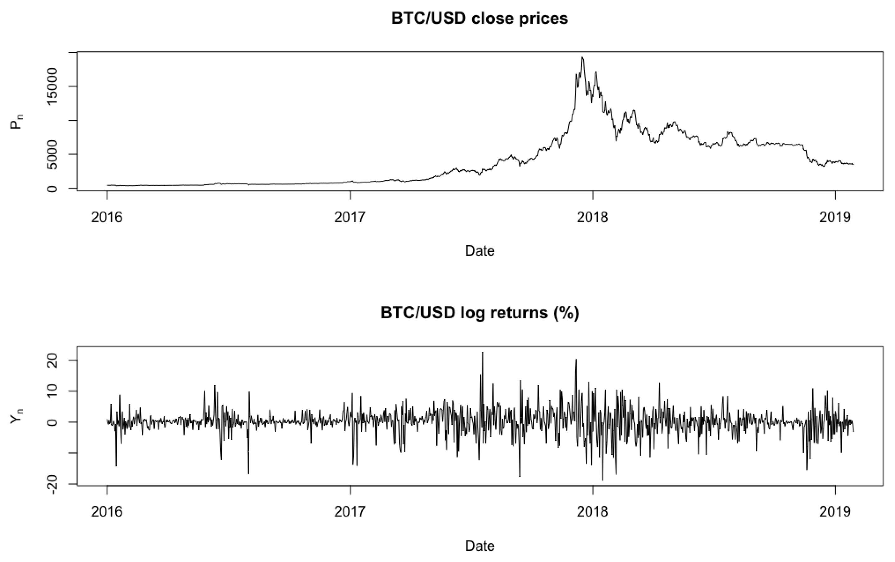
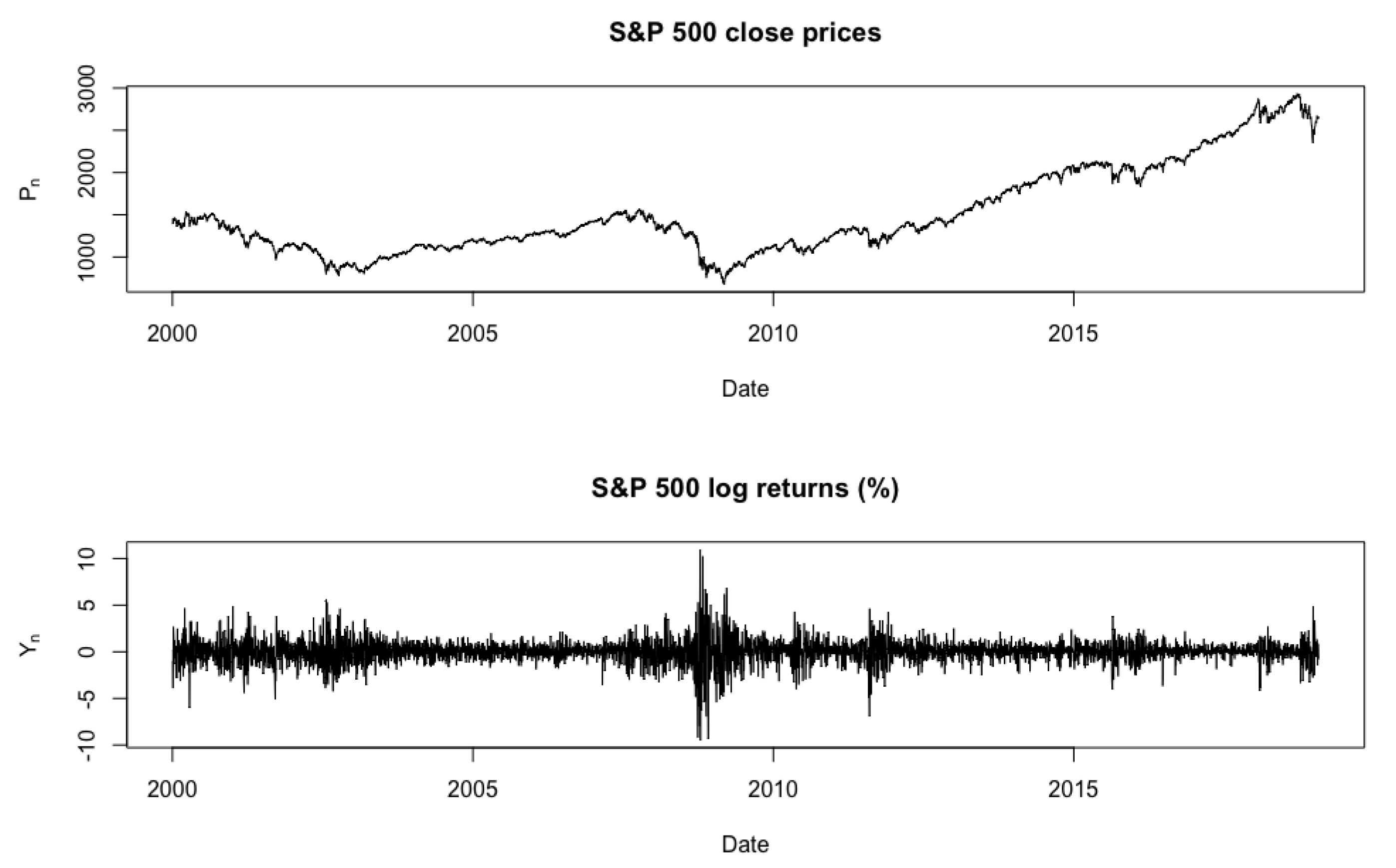
The aim of this paper is that of identifying market regime patterns of cryptocurrencies through the use of HMMs and HSMMs, where we assume that each state follows a Gaussian distribution with both parameters dependent on the states. Furthermore, we look into the evolution of the parameters of each distribution across time on a chosen test set. To test our models, we implement mock investment strategies on test data and compare this to a buy-and-hold approach to determine how well these regimes are identified. It is customary to say that when prices are on the rise for a relatively long period of time, the market condition is a bull market, and when prices fall steeply with respect to recent highs, the market condition is a bear market. Two other phases that may be found in the process are corrections and rallies, with the former being a period of steady decrease amid a bull market and the latter being a period of slow increase within a bull or bear market. It is possible that HMMs and HSMMs may struggle to distinguish between these two states due to the fact that neither is associated with a steep change. Due to a high correlation between movements of various cryptocurrencies, we focus on the daily closing prices of BTC/USD, the most mature cryptocurrency, for the dates ranging from 1 January 2016 to 28 January 2019, for a total of 1124 trading days. Bitcoin is around 50% of the cryptocurrency market. Since traditionally, positive trends with low volatility and negative trends with high volatility have respectively been labelled as bull and bear markets, we compare and contrast our findings with a de facto standard stock market—the S and P 500, where the dates considered are 1 January 2000–28 January 2019. This can be invested in collectively via the S and P 500 Index Fund.
The following is a review of existing literature related to cryptocurrencies and the use of HMMs and HSMMs to model financial assets. Starting with the former, Reference [
9] fit various parametric distributions on cryptocurrency returns. Furthermore [
10,
11,
12,
13,
14] fit GARCH models and its variants in their single-regime form. Reference [
15] looks at the application of Markov switching autoregressive models to Bitcoin. Recent publications that involve the modelling of Bitcoin volatility dynamics at multiple regimes are [
16,
17]—though different approaches were used for modelling in these papers with slightly varying results, in all cases, multiregime dynamics within a heteroscedastic framework were detected. Other literature in a different direction includes Reference [
18], which proposes a time-varying parameter VAR model that incorporates Bayesian shrinkage priors for the purpose of introducing regularisation in the model framework, and Reference [
19], which performs a Bayesian change-point analysis of Bitcoin. The following, on the other hand, are examples of literature using HMMs and HSMMs to model different phases of financial asset price movements. Reference [
20] shows that a normal HMM is capable of reproducing most of the stylised facts for daily S and P 500 return series established by [
21]. However, they only allow the standard deviations to vary by the state, while the means are fixed at zero. Recently, Reference [
22] applied a four-state HMM for stock trading by predicting monthly closing prices of the S and P 500, showing that the HMM is superior to the buy-and-hold strategy as it yields larger percentage profits under different training and testing periods. Modelling literature on financial time series using HSMMs is, however, quite limited. Reference [
23] compared HMMs and HSMMs when modelling the daily returns of 18 pan-European industry portfolios. They concluded that the HSMM with a negative binomial dwell-time distribution is a better alternative than the geometric distribution for HMMs. Reference [
24] implemented a three-state HSMM to describe the dynamics of the Chinese Stock Index 300 (CSI 300) returns. The authors assumed normal state-dependent distributions with logarithmic dwell-time distributions and also implemented a profitable trading strategy.
In this paper, what we aim to do over and above the cited literature is to assess how the HMM and HSMM methodology for market phase detection performs within the cryptocurrency context by looking at BTC/USD and also drawing comparisons with benchmark stock such as the S and P 500. Furthermore, apart from implementation on Chinese stock in [
24], the implementation of HSMM methodology on the S and P 500 or other traditional stocks has not been encountered in other literature we have reviewed. In the next section, we discuss the modelling approach implemented in this paper.
2. General Methodology
The daily adjusted close prices of BTC/USD and the S and P 500 were obtained for suitably chosen time periods, not equal in length, that encapsulate the swings the financial instrument goes through. Log returns of the daily adjusted close prices were taken, and the HMM and HSMM models were then fitted on the log returns. Mathematically, an
m-state HMM consists of two processes: (i) an unobserved (hidden) discrete-time
m-state Markov chain,
, taking values in a finite state-space,
, and (ii) a state-dependent process,
, whose outcomes (observations) are assumed to be generated by one of
m distributions corresponding to the current state of the underlying discrete-time Markov chain (DTMC). The distribution of
is assumed to be conditionally independent of previous observations and states, given the current state
. Such dynamics can be represented by the probabilities
and the mass/density function
the latter depending on the nature of the observations. For stationary HMMs, we denote by
the resulting stationary probabilities of the underlying DTMC. For a thorough review of HMMs, refer to [
25].
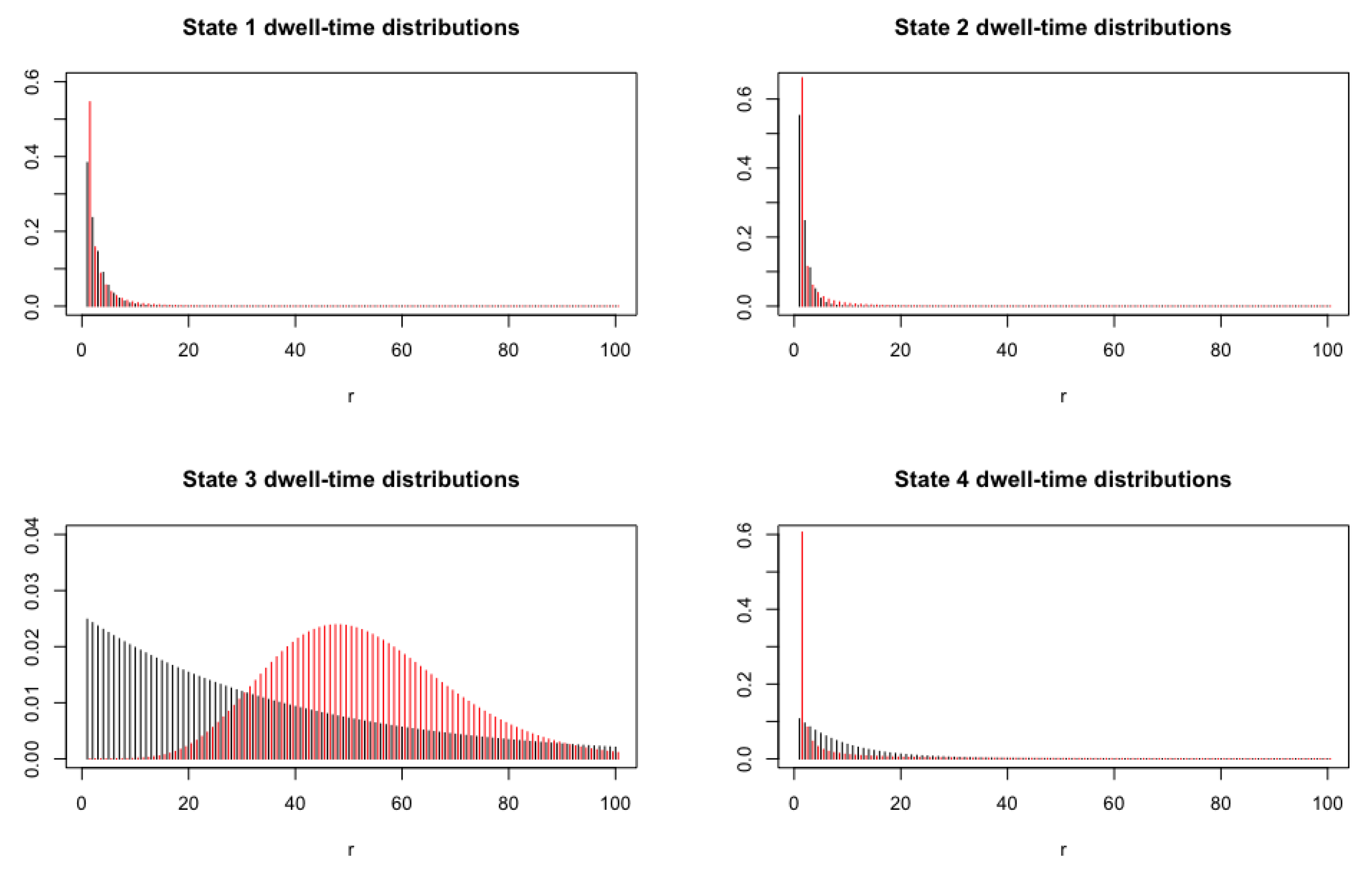
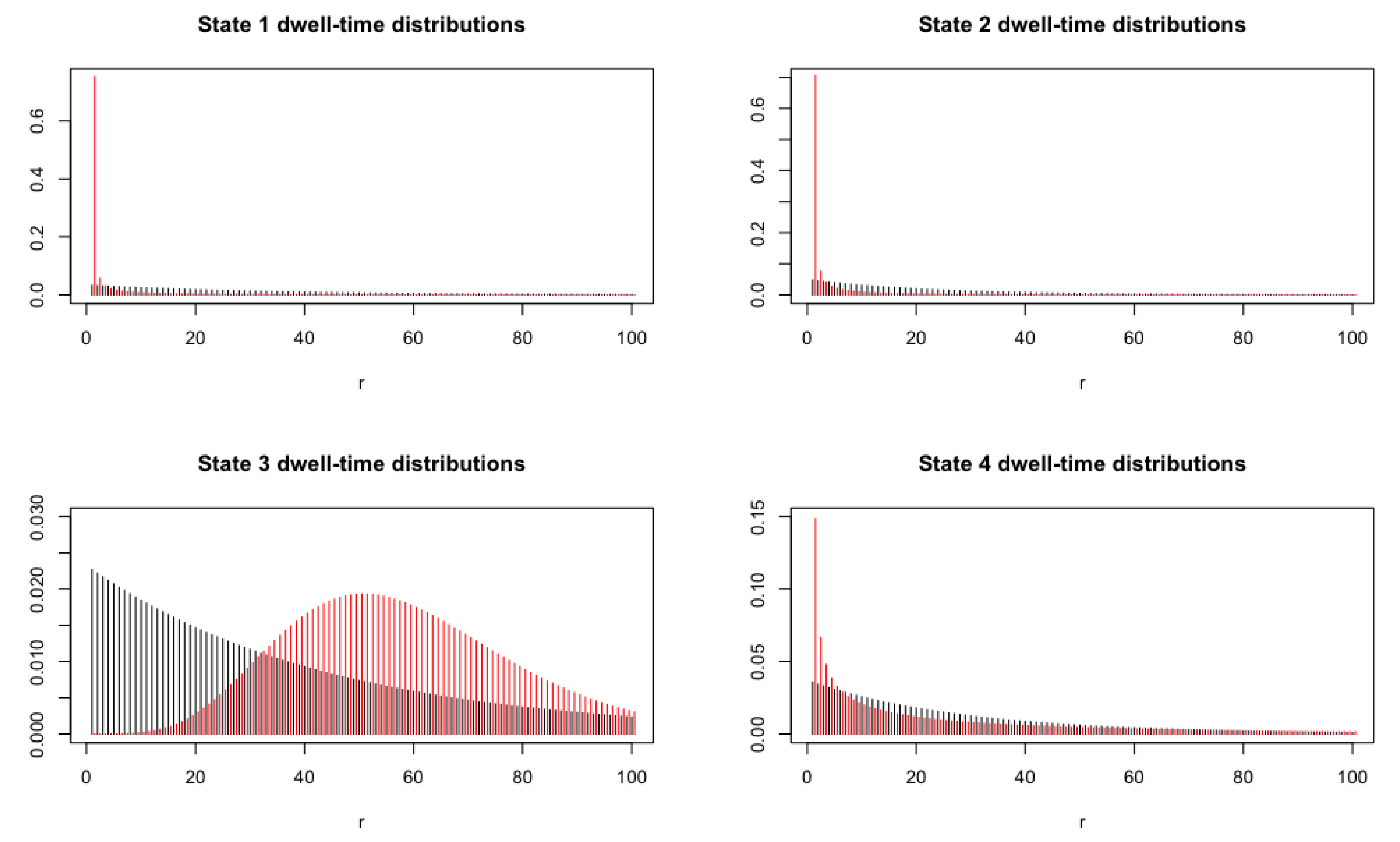
One drawback of basic HMMs is due to the one time lag memory of the underlying first order DTMC, which is inherently geometric. This means that the probability mass function of the dwell-time (i.e., the time spent) in state
i, denoted by
, is given by
. One possible way to circumvent this problem is to consider general state (not necessarily geometric) dwell-time distributions, leading to the HSMM framework. Thus, HSMMs generalise HMMs by explicitly modelling state persistence and state switches separately. This is achieved by considering a DTSMC,
with state-space
. The state-dependent process for HSMMs is defined in the same way as the HMM case. Thus, the only difference between HMMs and HSMMs lies in the hidden state process. In this case, we define
and let
be any discrete non-negative probability mass function. Finally, we denote by
the initial probabilities of the DTSMC. For a thorough account of HSMMs, refer to [
23] and references therein. Since the log returns take values in the real space
, we assume the state-dependent process to be distributed as normal with mean
and standard deviation
, where the
s and
s are the means and standard deviations for each state, for both HMMs and HSMMs. Moreover, the HSMM specification assumes that
is distributed as a negative binomial with parameters
, where the
s and
s are the negative binomial parameters for each state.
Parameter estimation of HMMs can be carried out by either direct numerical maximisation (DNM) of the likelihood via Newton-type methods or by the expectation maximisation (EM) algorithm. Both methods are described in [
25]. HSMMs are usually fitted via the EM algorithm as described in [
26]. For HMMs, the parameters we estimate are the
s, the
s, and the
s, while the
s are a direct consequence of the transition probabilities
(refer to Tables 2 and 5). For HSMMs, the parameters we estimate are the
’s, the
s, the
s, the
s, the
s, and the
s (refer to Tables 3 and 6). For HMMs, the Viterbi algorithm in [
27] can be applied for both HMMs and HSMMs to obtain a sequence of most likely hidden states. In other words, the aim of the Viterbi algorithm is to seek the particular sequence of states
that maximise the conditional probability
, where
N is the length of the series considered and
represents the state at time
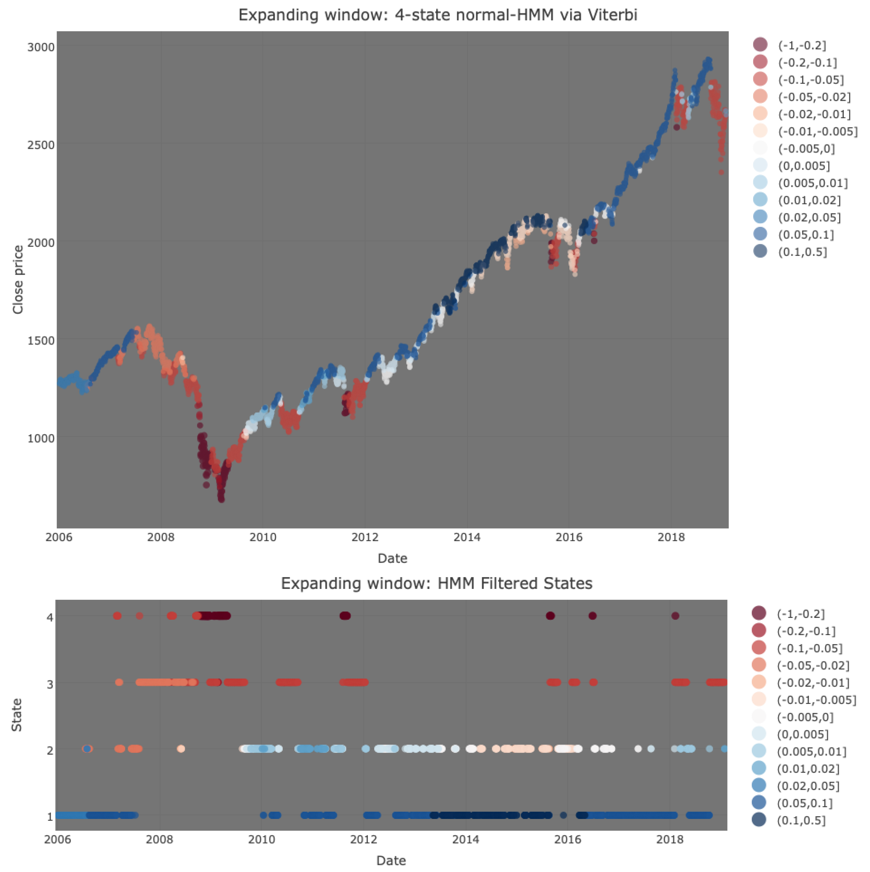
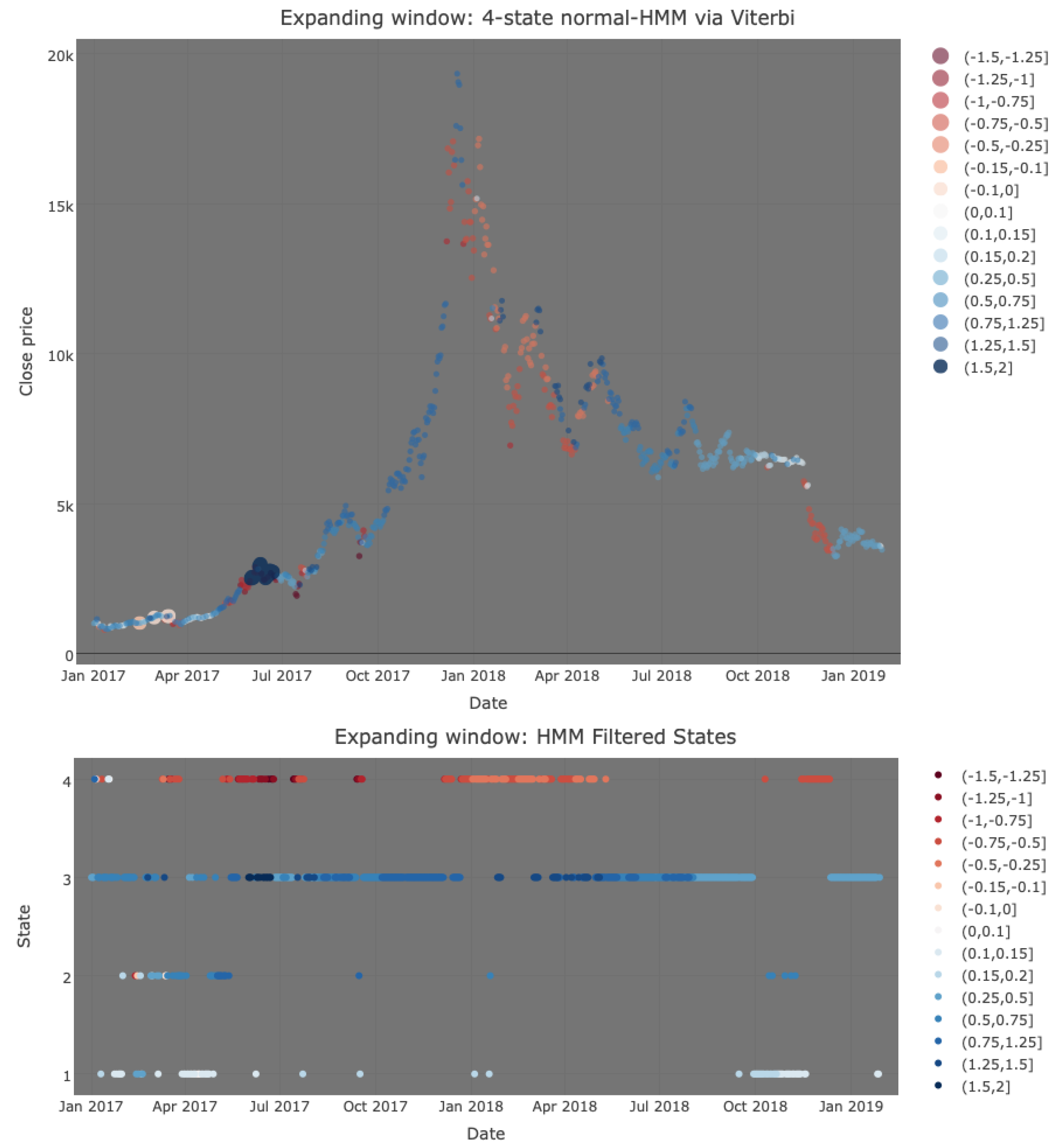
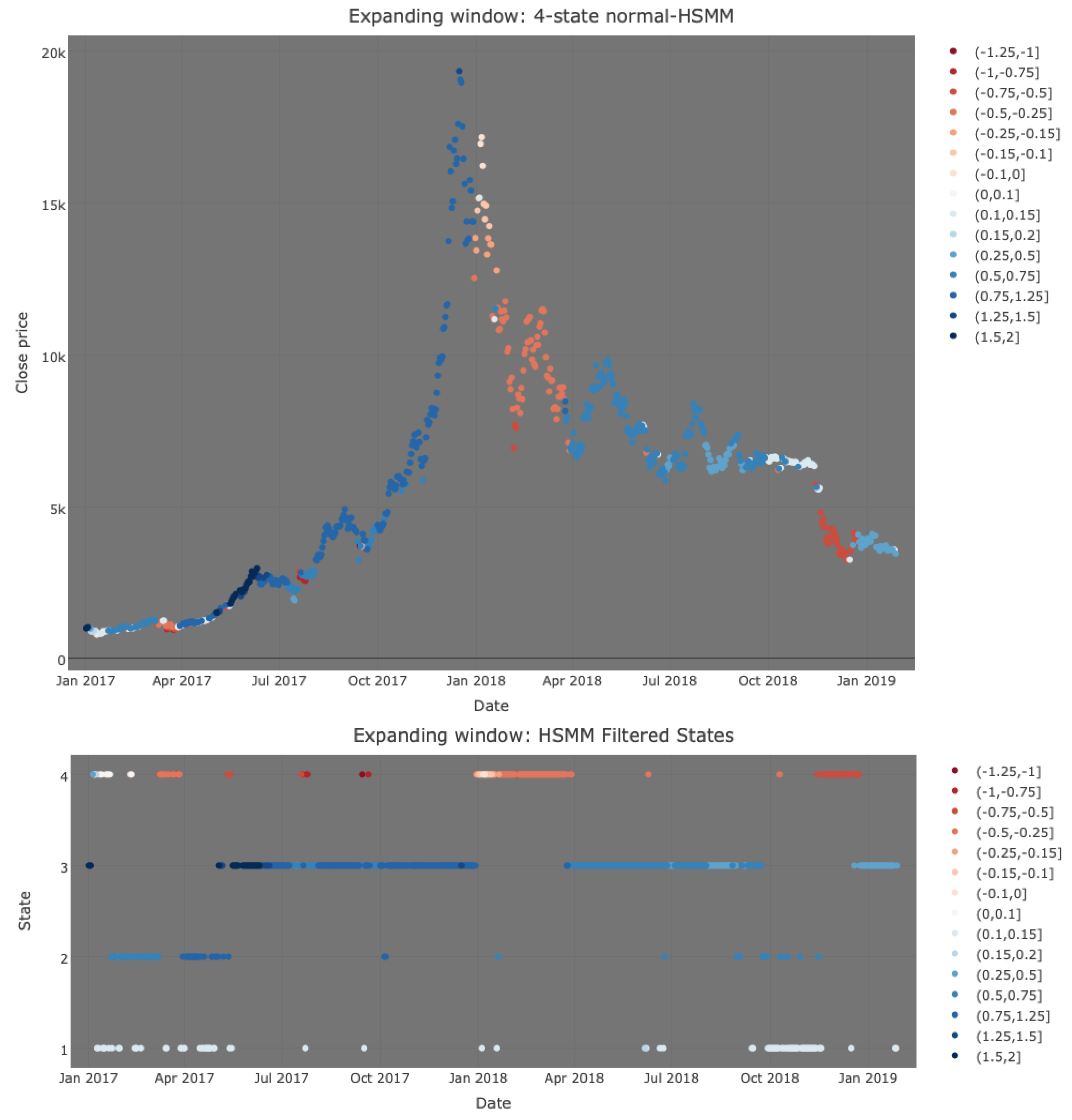
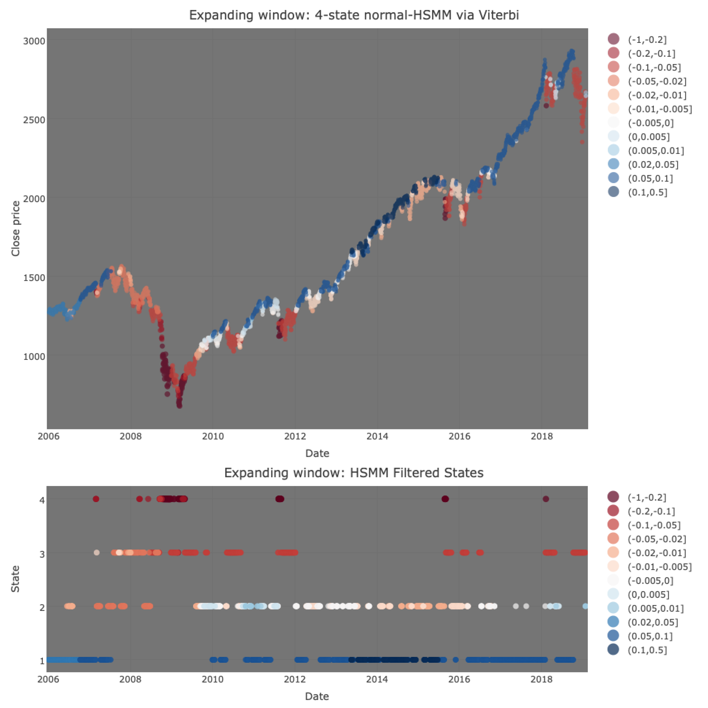
n. Hence, by labelling the order of the states according to the Viterbi algorithm, one deciphers the most probable market phases based on the entire observable sequence of log returns, which in turn guide us in making profitable investments. Such a procedure is called global decoding.
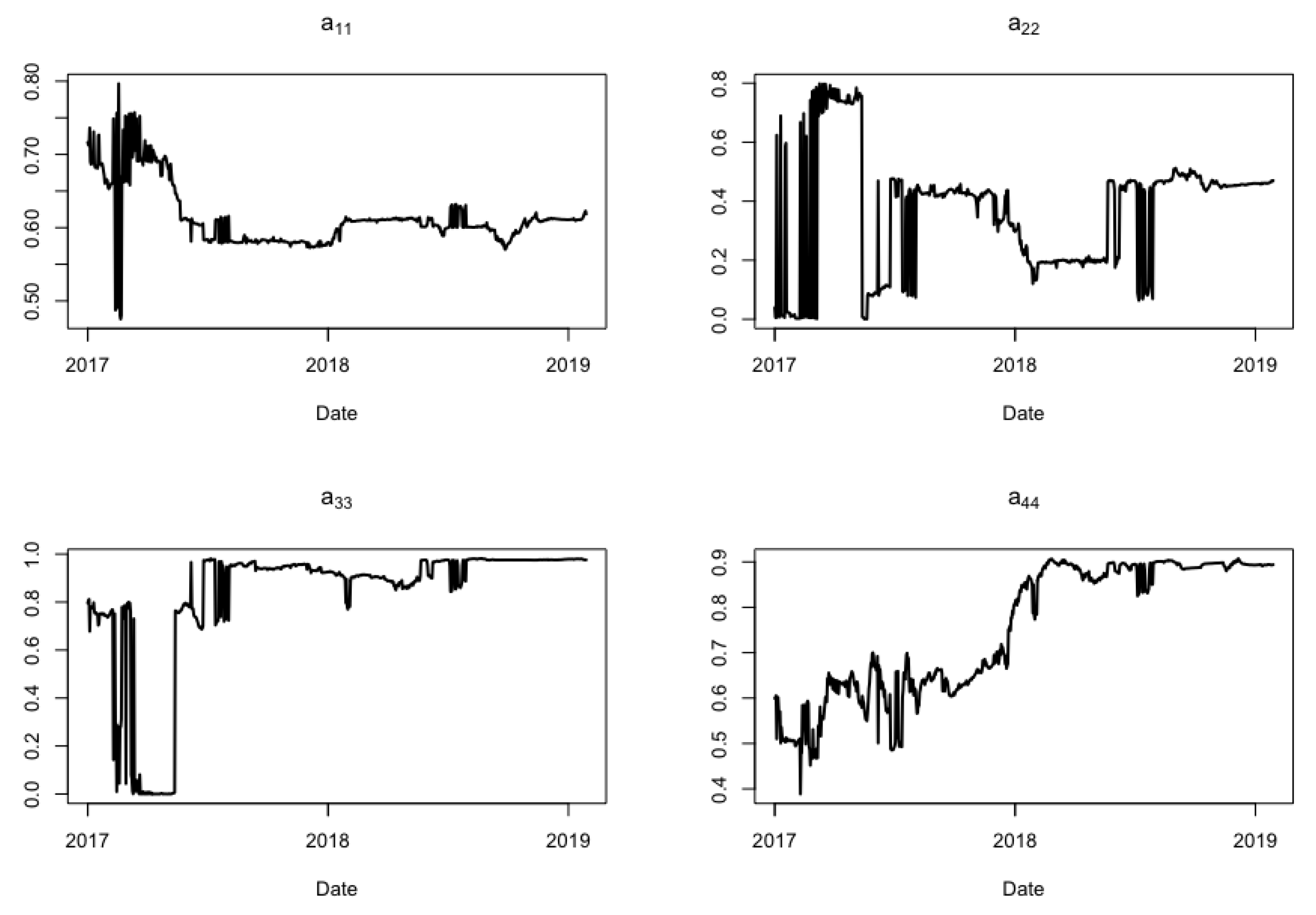
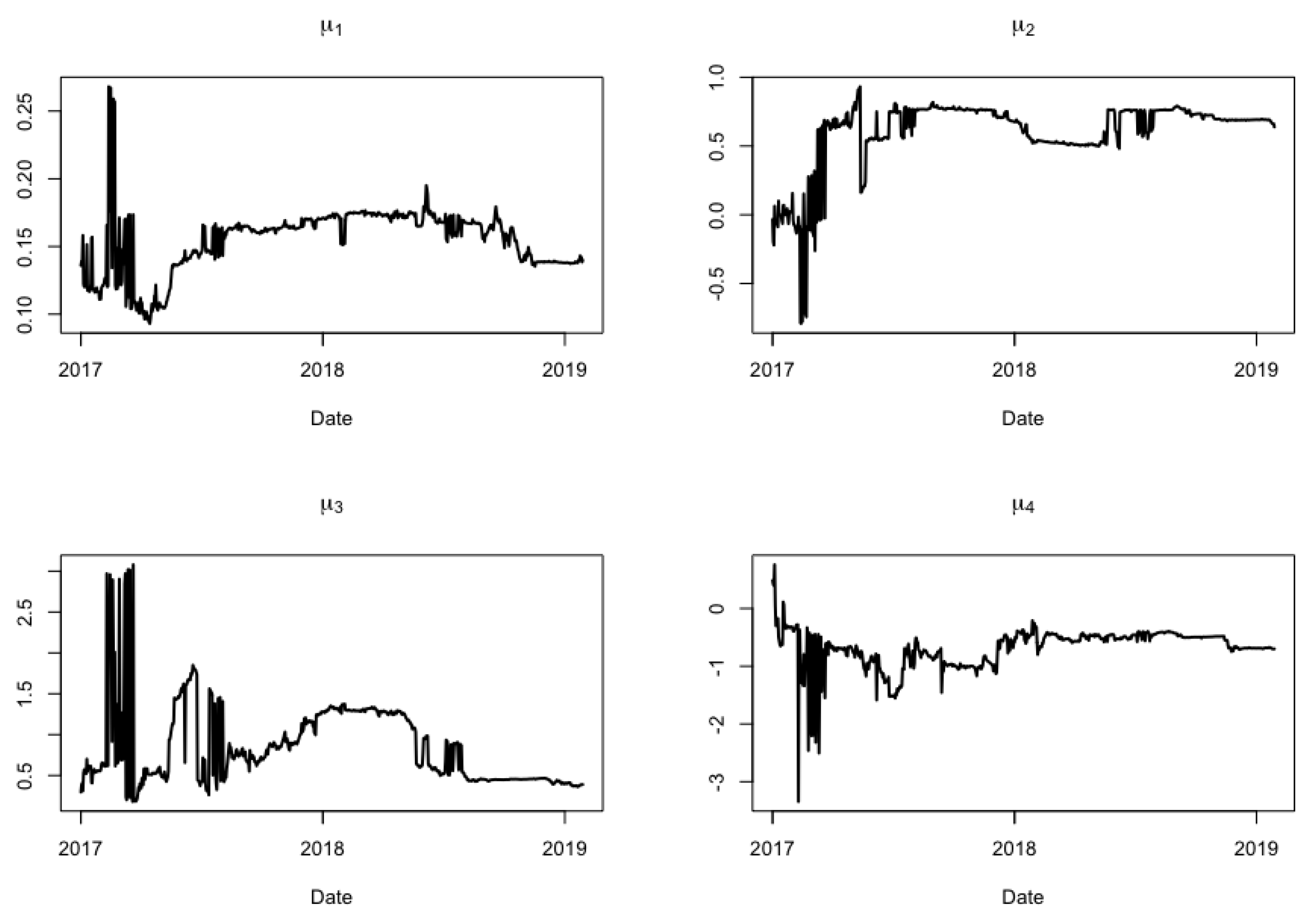
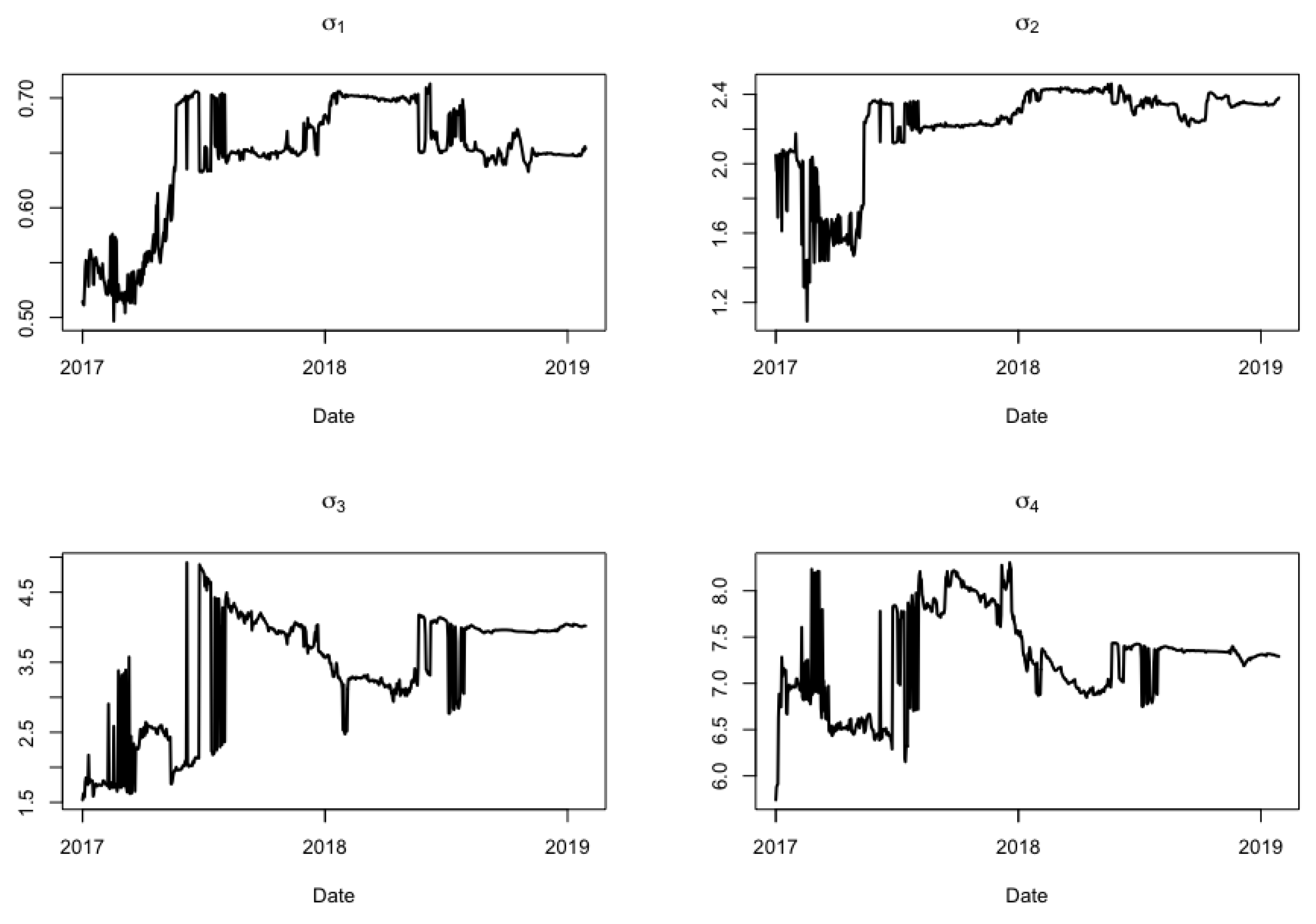
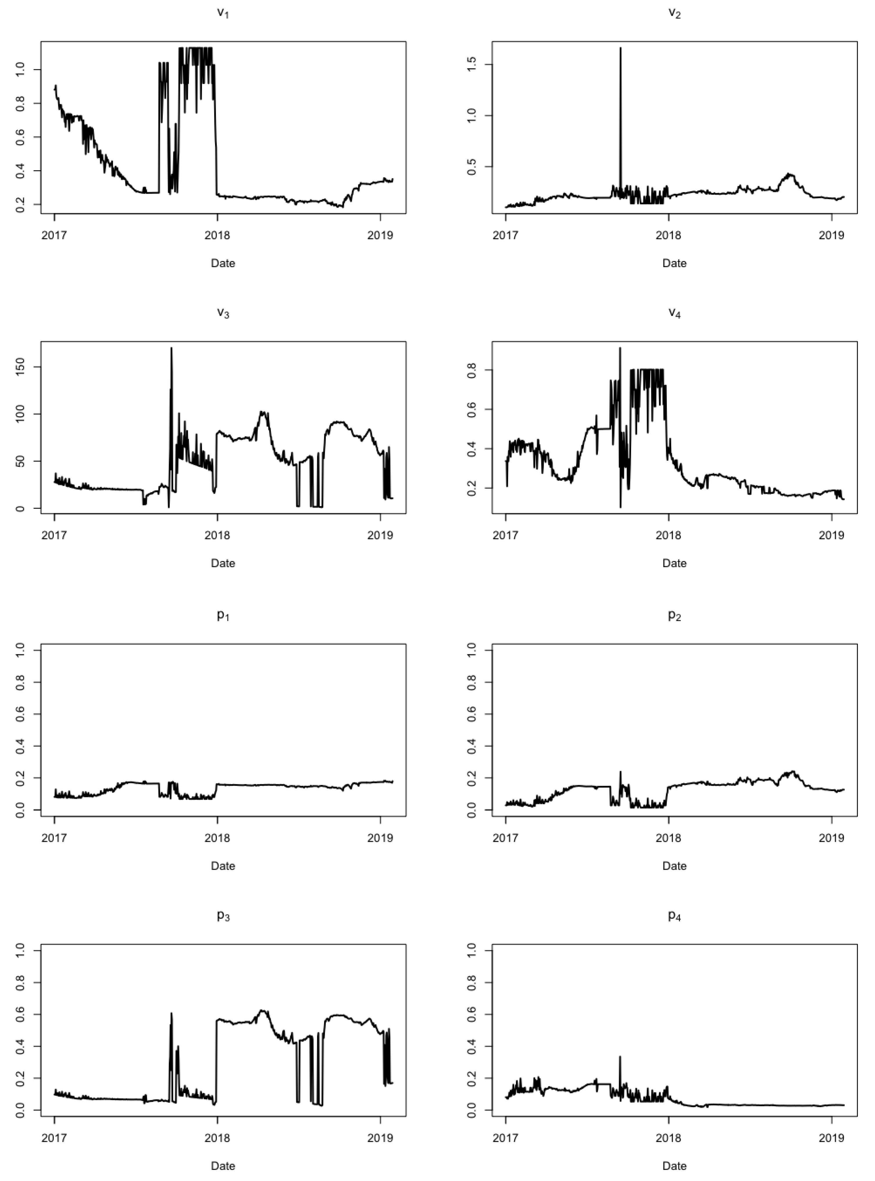
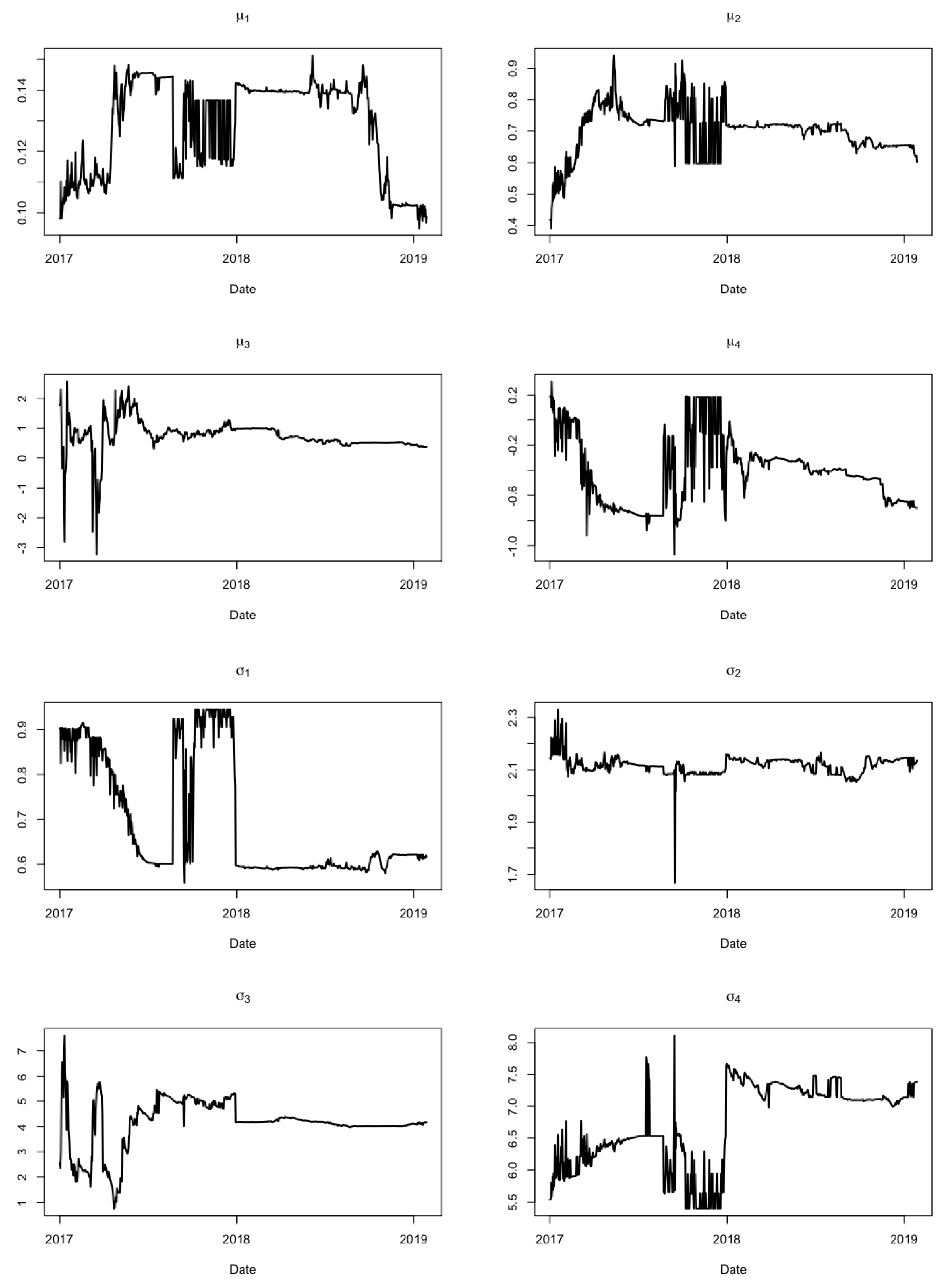
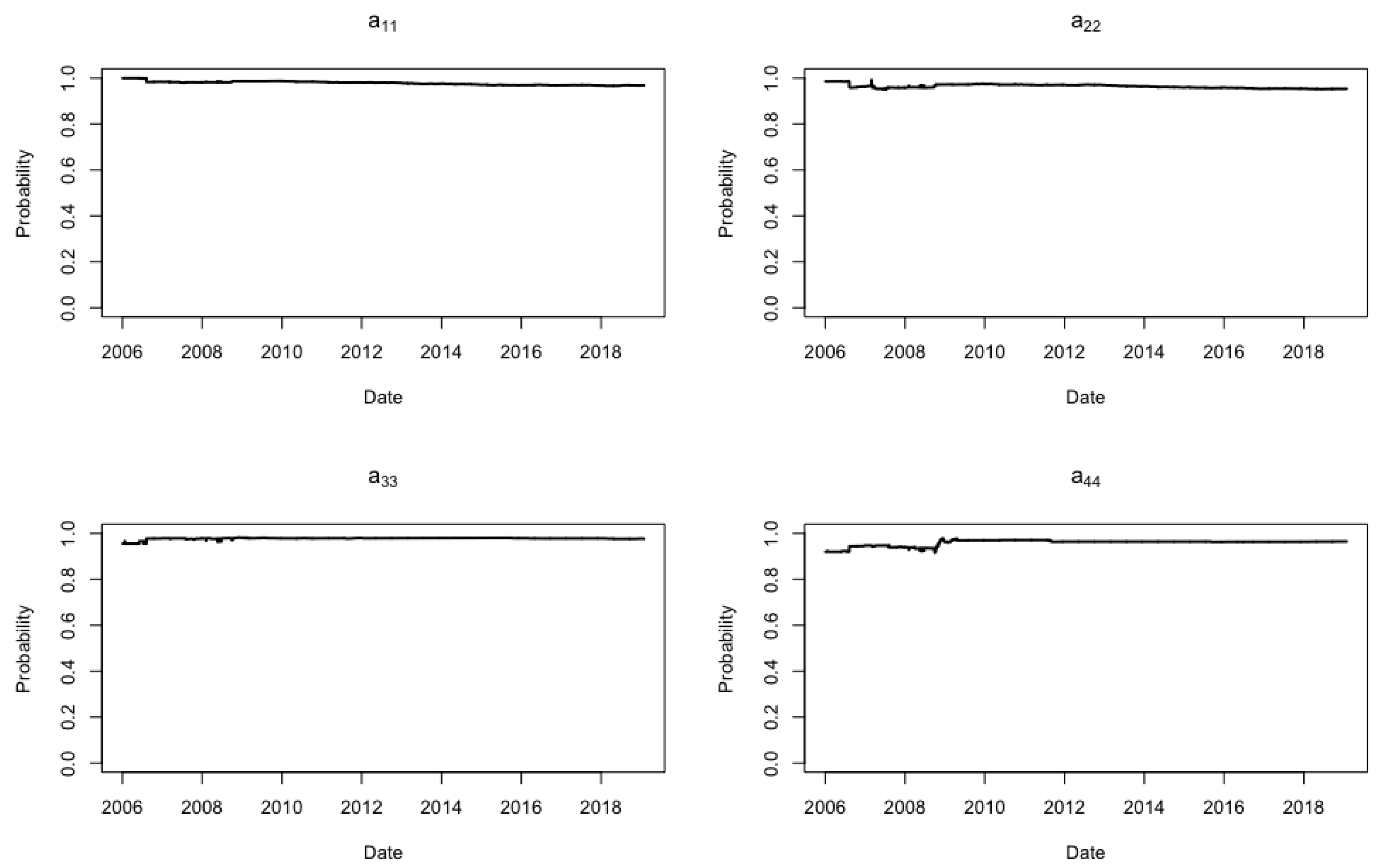
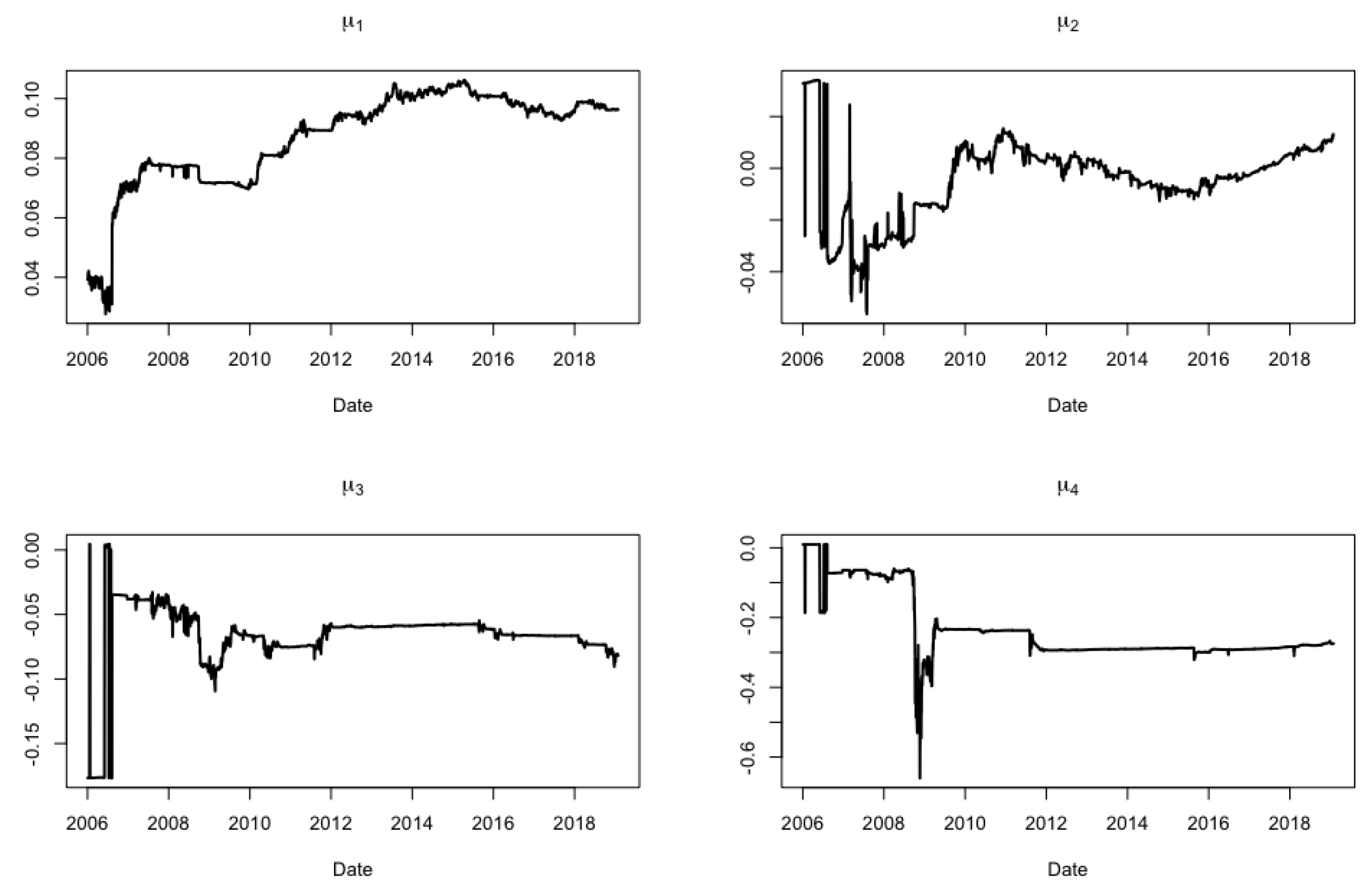
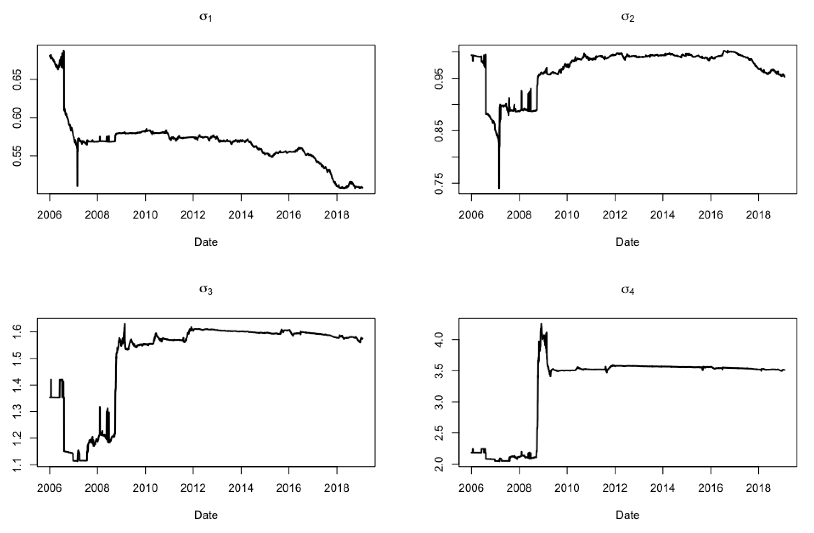
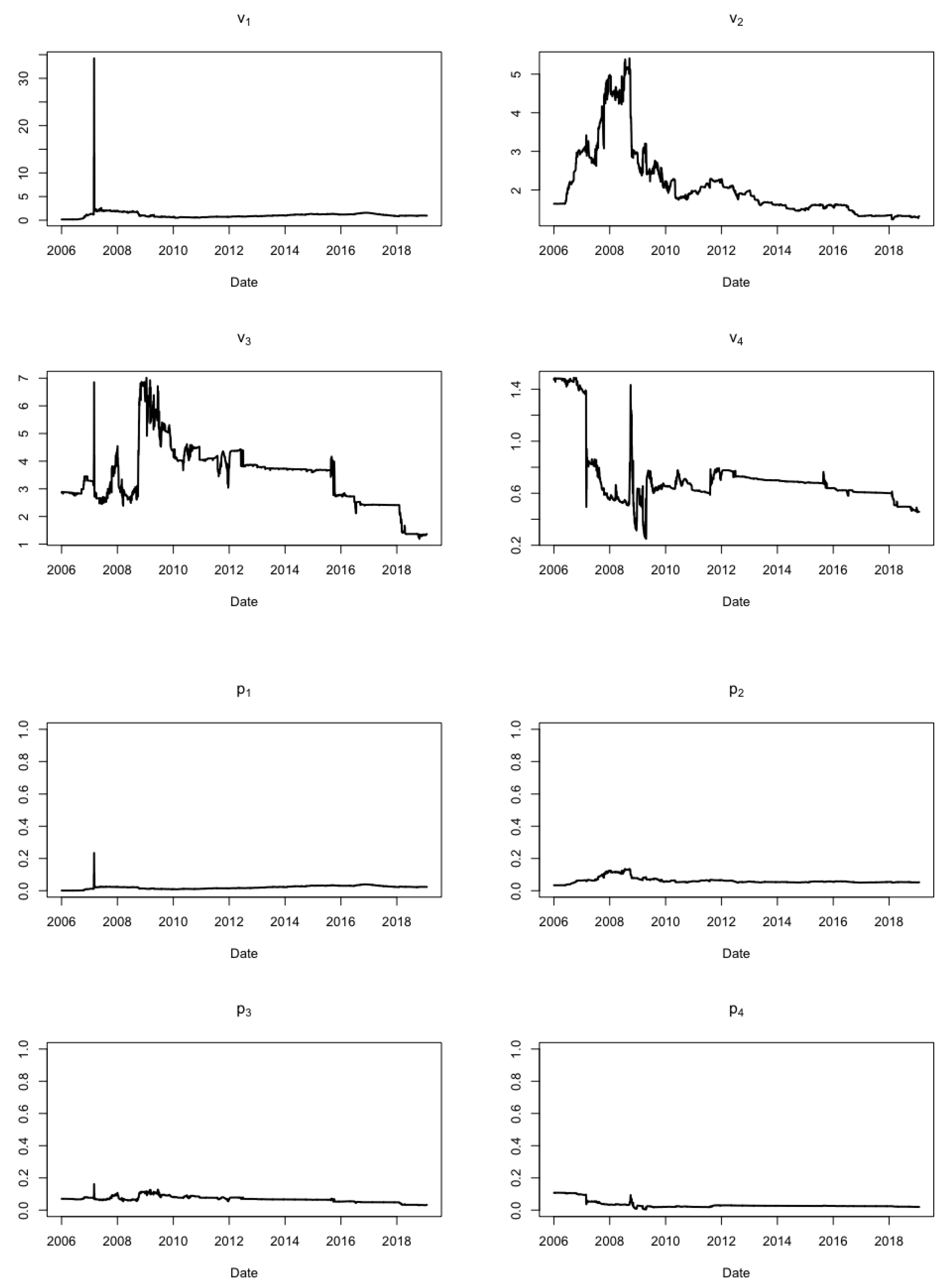
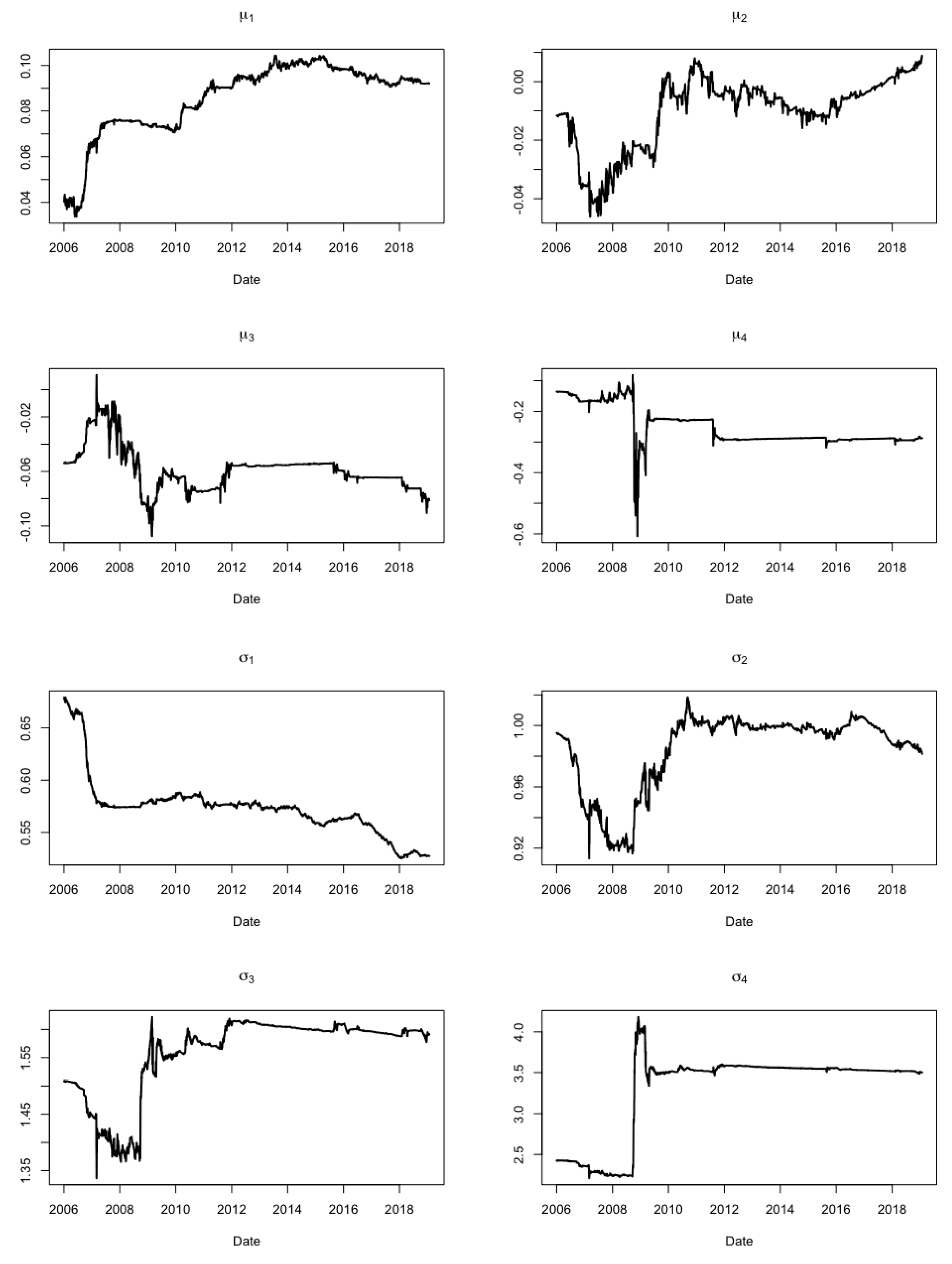
The daily log return series are hence analysed as follows: (i) suitable HMMs and HSMMs on the complete time series are fitted by varying the number of assumed states; (ii) the optimal model based on the Akaike information criterion (AIC), Bayesian information criterion (BIC), and Hannan–Quinn criterion (HQC) is chosen; (iii) the chosen time period is split into mutually exclusive training and testing periods; (iv) an expanding window method is implemented by first fitting the optimal model on the training set and then iteratively adding one time-point from the test set (until the testing period is exhausted) to the training period and applying the Viterbi algorithm as a filtering procedure to nowcast the current most likely hidden state after parameter re-estimation; (v) the evolution of the mean and variance parameters of each state across time are analysed on the chosen test set; and (vi) finally, investment strategies based on the model features arising from the Viterbi algorithm are applied to determine models’ success at determining market phases. The data analysis presented next was carried out using R packages
HiddenMarkov from [
28] and
hsmm from [
29].
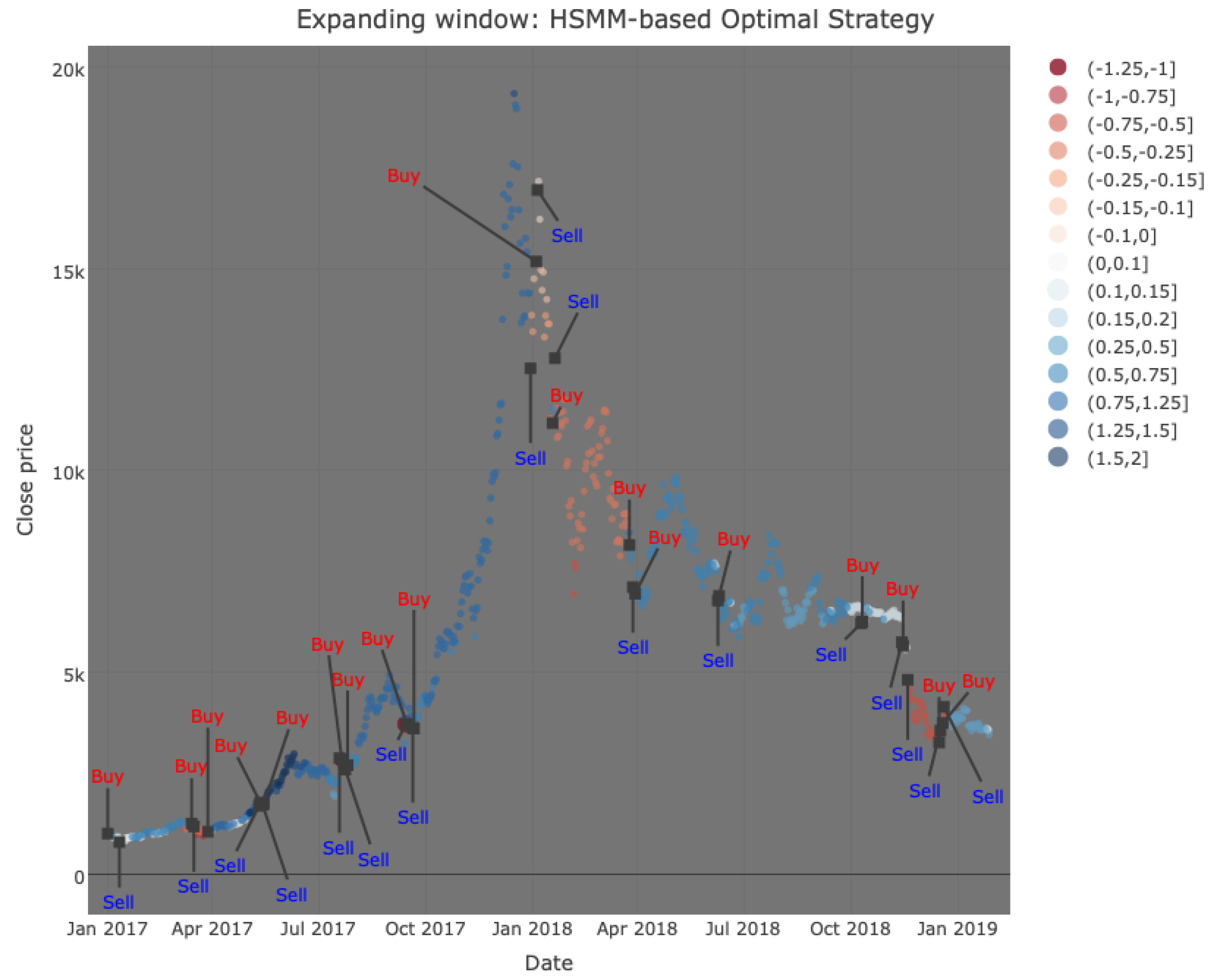
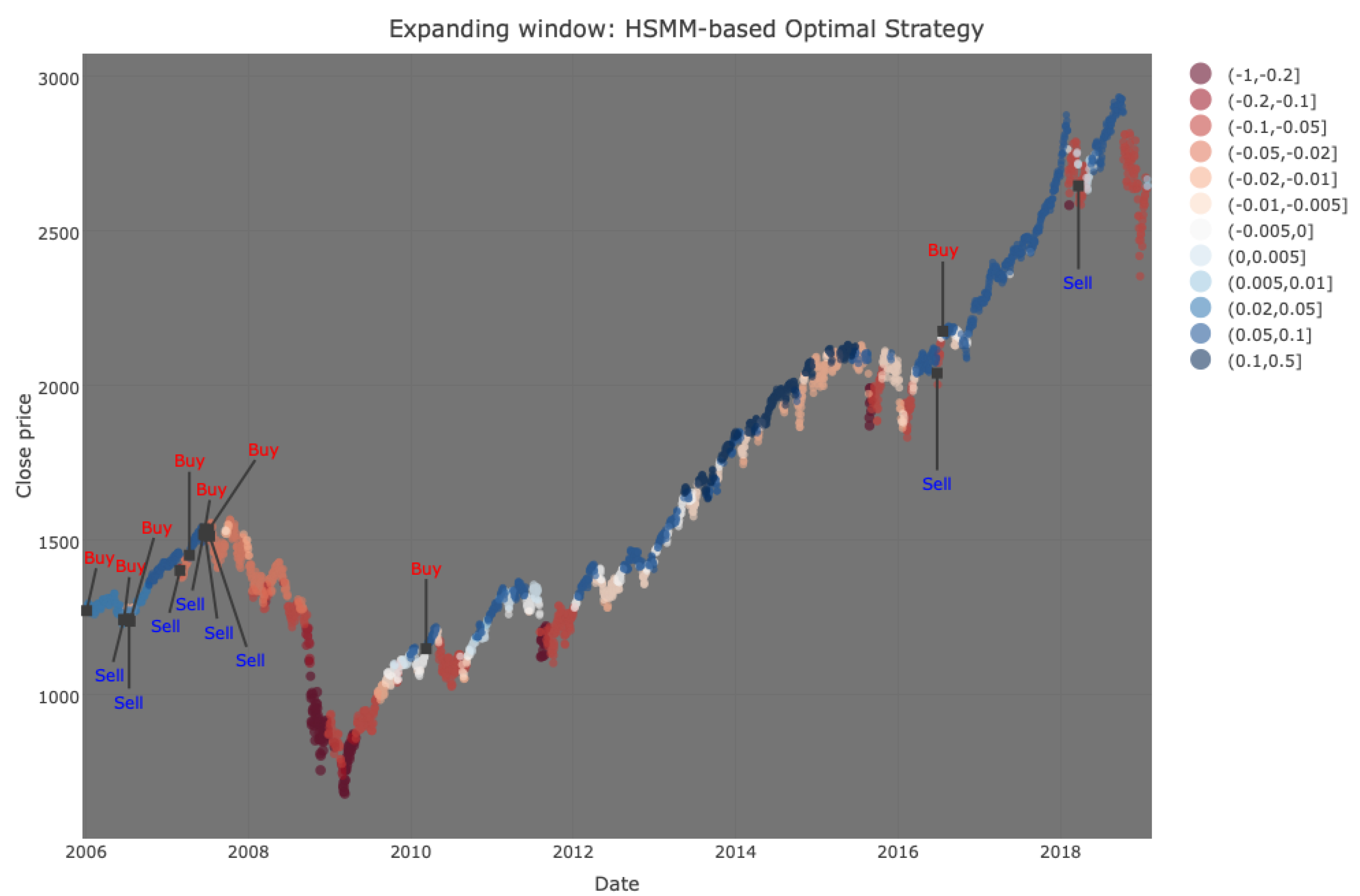
4. Investment Strategies to Assess Model Adequacy
In order to analyse the success of HMMs and HSMMs in determining bull and bear features, we devised four mock investment strategies and applied them with the expanding window procedure on both BTC/USD and the S and P 500, using the buy-and-hold strategy as a benchmark. For simplicity, the following assumptions were made for each strategy: (i) the actions (buy or sell) are not subject to transaction costs; (ii) the testing period is entered with an initial capital of $20,000; (iii) the first action is to buy on the first day of the testing period; (iv) if a buy signal is given, financial assets are bought only if enough cash is at hand; and (v) if a sell signal is given, financial assets are sold in their entirety if and only if they are owned. The first is a naive investment strategy called buy-and-hold, which is used for comparative purposes.
Strategy 1—Buy-and-Hold:
The buy-and-hold is defined by two actions:
The second strategy is based on the way we arbitrarily associate the states obtained via the Viterbi algorithm under the expanding window procedure (see earlier explanations for more detail).
Strategy 2—Regime:
At each state change given a particular time n, apply the following actions:
Given that state is associated with a bear market at time and state associated with a bull market at time n, buy as many financial positions as possible at time n.
Given that state is associated with a bull market at time and state associated with a bear market at time n, sell all financial positions at the close price of time n.
Otherwise, do nothing.
For Bitcoin, we consider state 3 as a bull state and state 4 as a bear state, while other states will not be labelled since they are ambiguous and infrequent. For the S and P 500, on the other hand, we shall consider states 1 and 2 as bull states and states 3 and 4 as bear states, based on the probabilities in connecting them. For the third and fourth strategies below, on the other hand, we denote the mean estimate by such that is the Viterbi chosen state at time n. Moreover, the following grid values for , based on empirical evidence, are taken: ; and , for BTC/USD and the S and P 500, respectively.
Strategy 3:
Given a particular time n, apply the following actions based on a pre-specified tolerance :
If and for , then buy as many financial positions as possible at time n.
If and for , then sell all financial positions at the close price of time n.
Otherwise, do nothing.
Strategy 4:
Given a particular time n, apply the following actions based on a pre-specified tolerance :
If , and for , then buy as many financial positions as possible at time n.
If , and for , then sell all financial positions at the close price of time n.
Otherwise, do nothing.
Note that strategies 2 to 4 are HMM/HSMM-based since they make use of the underlying hidden states or the active state-dependent normal distribution means. Strategy 2 can be interpreted as the simplest out of the HMM/HSMM-based approaches since it only considers information regarding the inferred hidden state sequence and the “subjective” interpretations attached to each state. Strategy 3 can be interpreted as an indicator of when a regime that is characterised by a negative trend is superseded by another regime that is characterised by a positive trend, according to some pre-defined threshold value . When , strategy 3 becomes a simple indicator of a negative-to-positive trend or vice versa. Thus, this strategy tries to capture bull–bear movements and capitalise immediately on such transitions. However, strategy 3 with is clearly susceptible to market correction traps since it does not consider the size of the trend. This led to the consideration of other that take into consideration the current estimated trend size. Thus, strategy 3 with could possibly improve upon the case when by ignoring buy (or sell) signals that are based on trends that are too close to zero. Thus, choosing an attempts to capture bull and bear phases by ignoring periods which are characterised by weak upward or downward trends that could potentially mislead investors in making unprofitable decisions. However, the aforementioned strategies are flawed in situations where state-switches occur in (unrealistic) short terms. As an attempt to limit this, we considered strategy 4, which builds upon strategy 3 by additionally taking into account the trend of the day before yesterday and waiting one day before performing an action. The one-day waiting time in a particular regime acts to safeguard excessive actions during turbulent periods where the models infer consecutive (unrealistic) state-switches.


