Abstract
This paper applies a methodology for computing external costs in an intermodal transport network that includes short sea shipping to explore the impact of external costs in its competitiveness. The network, which includes roads, freight railways, maritime and inland waterway connections, considers the specific characteristics of different transport alternatives and vehicle types, providing a fair comparison of the various modes. A case study focused on freight transportation between Northern Portugal and 75 destinations (NUTS2 regions) in north-western Europe is presented. The potential of different intermodal routes that include short sea shipping is assessed, including not only internal costs and times but also external costs per mode and unit of cargo. The impact of the different cost approaches in each country of transit is shown along with the progress that has been made in the integration of external costs, using the most recent EU estimates on marginal costs coverage ratios per country for freight transport modes. The results support the modal shift from road to sea in this corridor, providing means for modal comparison and for the development of short sea shipping’s image as a sustainable mode of transportation.
1. Introduction
Transport activities impose costs on society and the environment that are not fully taken in consideration in the decision-making process of transport users. Apart from the impact of air pollutants and greenhouse gas emissions (GHG), which have been tackled over the years by policies and regulations at the EU and international level, other costs, such as congestion, accidents or noise costs, are only now starting to be addressed, and this occurs when, at the same time, transport demand is set to triple in the next 30 years. This increase in transport volume will also result in an increase in congestion costs by about 50% in 2050, as well as an increase in the costs of accidents and noise [1].
Road freight transport is responsible for the largest share of total external costs of transport in the EU, contributing significantly to road degradation, air pollution and including a significant number of fatalities from accidents. However, over 70% of freight transport is still road based. For that reason, a substantial modal shift of freight transport from roads to other modes of transport has been one of the key objectives of the EU transport policy [2,3].
Multimodality in freight transport is an answer for long distances and needs to become attractive for shippers. While rail can be an attractive mode, the large investment that is still needed to upgrade the rail network in Europe place it after waterborne alternatives in peripheral countries such as Portugal. The sustainable mobility strategy of the European Commission (EC) now includes an increase of 25% by 2030 of inland waterways (IWT) and short sea shipping transport (SSS) and of 50% by 2050 [3]. The same strategy recognises that the impacts of transportation must be fully included in its prices as a necessary and crucial step in the development of a greener, more efficient and fairer transport system.
The EC has recently stated [2] that the full impact of transport may only be accounted for through the internalisation of external costs, implementing the principles of ‘polluter pays’ and ‘user pays’. Internalising means making the transport user accountable for the full costs of his transport decisions. This is to be achieved through carbon pricing (EU ETS, emission trading scheme) and infrastructure charging mechanisms. The first will cover the societal costs associated with CO2 emissions, while the second will cover the cost of damage to infrastructure, air pollution and congestion, inter alia. In this respect, the following milestones have been included in the EU strategy [2]:
- (i)
- By 2030, rail and waterborne-based intermodal transport will be able to compete on equal footing with road-only transport in the EU40, in terms of the share of external costs internalized.
- (ii)
- All external costs of transport within the EU will be covered by the transport users at the latest by 2050.
The most famous example of the introduction of those taxes and charges to cover part of the transport-related external costs is the Eurovignette system for the application of user charges for heavy goods vehicles in the EU that cover infrastructure costs, and in some cases air pollution and noise costs, used in Belgium, Denmark, Luxembourg, the Netherlands and Sweden. Unsatisfactorily, it represents only 20–25% of the European transport network. The Community of European Railway and Infrastructure Companies (CER) has called for an update on the Eurovignette Directive to be more widely applicable, thus making the competition between road and rail fairer, stimulating the modal shift and its benefits in terms of reducing greenhouse gases and societal impact [4]. The European Platform for Electro-Mobility, which includes representatives of other transport modes, has made similar calls [5]. Recently, CER has argued that the wide application of those principles in the transport sector in the EU is also a necessary measure to finance the economic recovery from the coronavirus pandemic, as it could help raise over €300 bn per year [6].
At the European level, the latest version of the Handbook on external costs of transport [7] provides the state of the art regarding the calculation methodology and external cost figures, in €-cent/tkm and €-cent/vkm. These can be used to estimate the costs associated with a particular transport chain and assess its internalisation. However, it has been estimated that including external costs in the economic assessment of alternative transport chains can make SSS-based chains competitive and attractive for shippers in new transport corridors [8,9]. An analysis on the state of the art of external costs of inland waterways and maritime transport concluded that the number of papers dealing with those modes are rather low when compared to road transport [10]. Another recent study on the research gaps on the comparison of SSS with road transport [11] emphasizes the need for the development of detailed cost models that can be applied in route-specific research and include the external costs of transport. The research on cross-modal comparisons for different transport corridors is important because only when considering the specific characteristics of those corridors can there be a fair comparison of the various transport modes [12].
This paper contributes to fill these research gaps by evaluating the economic performance of the intermodal chains that include SSS versus those of road and rail freight transport, comparing the total societal costs of transport (internal plus external costs) in a specific transport corridor and finding answers for the following research questions: Which types of external costs are more important for each transport chain? What is the quantitative relevance of external costs when compared with internal costs? Do external costs, when internalised, really promote multimodality?
These questions will be considered in more detail for the Atlantic Corridor extending from Portugal to Northern Europe, as it has been found that, in the European Union, Portugal comes second in the share of external costs of inland transport modes in the national gross domestic product (GDP), most of those coming from road haulage [7]. This is probably a consequence of the peripheral location of the country in relation to the centre of the EU. The numerical results presented in this paper are based on a general-purpose computational tool developed to estimate the internal and external costs in any transport corridor forming part of the Trans-European Transport Network (TENT-T). The numerical model has been presented before [13,14] and a detailed methodology is used for the estimation of the fuel consumption and emission quantities, which includes the effect of congestion in speed, the impact of new fuels and abatement technologies, particularly in maritime transport, and is based on the most recent emission inventories for all transport modes [15].
The lack of route-specific results for external costs for all transport modes made the comparison of costs and validation of the tool very challenging. Nonetheless, there are some works on the application of the European external cost factors on alternative road and sea routes, which made the validation possible [9,16]. The numerical results can also be compared with those from the MAE External Cost Calculator, designed in the context of the MED ATLANTIC ECOBONUS (MAE) project. However, all previous works are based on an outdated version of the European Handbook on External Costs of Transport [17] and none has been found based on the updated cost figures.
The structure of this paper is as follows. In Section 2, the types of external costs of transport are defined and it is discussed how those are accounted for in the literature. The current degree of internalisation of those costs in Europe is assessed. In Section 3, a summary of the numerical model behind the computation of external costs in an intermodal transport network is presented. In Section 4, alternative transport chains between Porto and Stuttgart are chosen and the results for all external cost types associated with those are shown in €-cent/FEU per chain, transport mode and for the country and geographical space under study, when applicable. The preference in terms of transport chain regarding external costs is compared with the preference in terms of internal costs and finally the total societal costs of each transport chain are compared. This analysis is then repeated for a set of 75 different destinations in Northern Europe. Conclusions are presented in Section 5, focusing on the value of the type of results obtained and on the main findings of the case study.
2. External Costs: Types and Degree of Internalization
2.1. The Concept and Types of External Costs
The concept of external cost is not new in economics: it was developed by British economist Arthur Cecil Pigou (1877–1959), who published the book Economics of Welfare in 1920 [18]. The concept had actually already been proposed by another notable British economist, Alfred Marshall. It may be defined as a cost or benefit that is imposed on a third party who has not agreed to incur that cost or benefit. The cost or benefit is not compensated, or fully accounted, by the party (social or economic activity) who has originated it. Since its origin, many other economists, such as James Meade, Ronald Coase and James Cheung, have since conducted further research in this field.
Externalities may be negative or positive and consumption or production related. Transportation is a sector know to produce significant negative externalities (external costs). In the EU handbook [7], these external costs have been divided into a number of categories: accidents, congestion, noise, air pollution, climate change, well-to-tank (WTT) emissions and infrastructure. For internalization and assessment of transport economic efficiency, marginal cost figures are used, instead of total or average external cost figures, because those represent the external cost increase caused by adding one more vehicle to the system. This means that we are only considering variable external costs, leaving out the fixed negative externalities, such as habitat damage. The types of external costs considered for each transport mode in the network are shown in Table 1.

Table 1.
External costs considered per transport mode.
The costs mentioned in Table 1 are defined in the EU handbook [7] as follows. Accident costs represent the parts of material costs, medical costs, production losses, suffering and grief caused by fatalities, which are not covered by the insurance of the person exposed to risk. When an additional vehicle joins the traffic, the driver is exposed to the average accident risk and changes the accident risk of the other transport users. For freight maritime transport the accidents costs are not included because those are only available for selected ports and in general represent less than 0.001% of a country’s GDP, since although they can have significant impact, they are also extremely rare. Congestion costs represent time costs, reduced reliability costs and missed economic activities due to the reduction of utility when using a road with a determined capacity. When a transportation company decides to use a road to move cargo from origin A to destination B, it is affecting the volume of traffic in that road and therefore the utility of all other users who wish to use the same road capacity. No illustrative quantification of congestion external costs for rail, inland waterway and maritime transport is available, so they are not quantified in the handbook. Furthermore, for IWW and maritime transport congestion is only an issue in selected ports (more often outside the EU). Noise costs represent the effects of noise exposure on people’s life, especially in urbanized areas, such as annoyance and effects on productivity, leisure and health. The impact of noise from shipping while at sea is assumed to be zero as well as for inland navigation.
Air pollution costs reflect the impact of air pollutants on human health, focusing on particulate matter (PM) (mostly fine PM2.5 from exhaust emissions), nitrogen oxides (NOx) and sulphur dioxide (SO2). The monetarization of those emissions is done using the damage cost in €/kg emission for each pollutant inland and at sea. In addition to air pollution, the handbook also considers the climate change costs, which reflect the impact of greenhouse gas emissions (GHG), namely, CO2, but also CH4 and N2O, and its impact on ecosystems, human health and societies. Emission quantities are estimated in terms of CO2 equivalents and the avoidance cost of those emissions are used to monetize them. Different monetarization approaches and prices, quite scattered [19], have been used in the estimation of climate change costs.
Well-to-tank (WTT) emissions are the upstream costs of energy production. Those represent emissions of air pollutants, greenhouse gases, other toxic substances and environmental risks for which there is a well-developed basis for monetization. Finally, marginal infrastructure costs are the only part of the renewal and maintenance costs associated with the variable use of infrastructure, i.e., the wear and tear costs. Those can be added to the external costs because those represent the impact of an additional vehicle in the network. Specific values are reported for different types of roads, trucks and trains. For waterborne transport, there are reported values for some countries and specific ports that cannot be considered generically and therefore will not be included in the model.
For maritime transport, the most important external costs, as mentioned before, are air pollution and climate change. However, all the other types of costs mentioned before are associated with intermodal chains based on SSS, because of its non-maritime legs. Studies on the hierarchy of transport externalities are emerging [20], linking the negative externalities of transport and supporting the development of sustainable mobility strategies that tackle the externalities with greater overall influence on society and the environment.
Furthermore, in port areas, external costs originate not only from ships but also from other modes connecting the ports with the destination as well as from cargo handling equipment [21]. For the populations around ports, noise created by the hinterland transport is the most visible externality, not from the ships but from trucks and trains. In fact, hinterland transport making use of roads creates external costs that may jeopardize the utilization of seaports [22].
Many studies have dealt with external costs of transportation, some of them containing evaluation methods for external costs arising from intermodal transportation [23]. Other papers focus on gains in terms of external costs obtained from an increased utilization of short sea shipping and comparisons between different intermodal transport chains [9,16,24]. These three papers focused on specific transport corridors in the West Mediterranean Sea, Baltic Sea and Aegean Sea. However, recent studies have emerged focusing on the external costs of transportation across port hinterlands, aiming at identifying the optimum locations for inland ports [25] or at optimizing transport operations in the distribution of containers [26], both taking in consideration not only the internal costs but also external costs of transportation.
2.2. Degree of External Costs Internalization
When external costs are not included in the cost of transportation, competition between modes is unequal and it can result in preference for modes that are more harmful to the health and safety of the people and the environment. This occurs because transport users only take part of the societal costs into account when making a transport decision, resulting in outcomes that are not optimal from the point of view of the society.
It is important to recognize that some limited progress has been made in internalising the external costs of transport. When studying the economic competition of different transport alternatives, this needs to be considered so that the analysis is not distorted. Market-based instruments such as taxes and charges are the main instrument recommended by the EC for the internalisation of external and infrastructure costs. The ‘polluter-pays’ and ‘user-pays’ principles are often emphasized, as occurs in [3]. Apart from generating revenue, these principles aim at a more efficient and fair transport system, increasing safety and levelling the competition between transport modes.
A report named the State of play of internalisation in the European transport sector [12] collected marginal taxes/charges corresponding to the variable part of taxes and charges that are directly linked to the use of transport vehicles and infrastructure. Those include fuel/energy taxes for all modes; road tolls, vignettes, tolls for bridges and tunnels in road transport; infrastructure access charges and the Emissions Trading Scheme (ETS) for rail; and port charges, fairway dues, dues for locks and bridges and water pollution charges in the waterborne modes. The marginal social cost pricing is theoretically considered as the number one approach to develop internalisation measures. This principle is applied when the transport user is charged with a sum equal to the marginal external (and infrastructure) costs, implying that the user is taking the cost of its transport decisions as it does with private costs. This was the approach used in the Eurovignette Directive [27]. In the case of shipping, the fact that this is an international market makes it harder for a particular state to enforce policies and it is not clear which entity should be responsible for it.
Currently, the degree of internalization of external costs in the EU is different for every transport mode, which again puts in question the fairness of the current transport system [28]. For freight transport, the cost coverage ratios for the variable external costs (accidents, air pollution, climate, noise, congestion and WTT) and infrastructure costs are 62% for diesel trains, 37% for electric trains, 33% for trucks, 13% for IWW and 4% for maritime transport, respectively [12]. However, for maritime transport, that ratio is based on values for a set of 34 EU individual ports and may not reliably represent what happens in some countries, as is the case of Sweden. Sweden (as well as Finland and Estonia) already differentiates the fairway dues according to the environmental performance of ships and there are studies that indicate that ship movements within their national waters have coverage ratios of at least 50% of the associated external costs [29].
3. Methodology
The methodology developed to estimate the external costs of transport in intermodal voyages, including short sea shipping, road, rail and inland waterways, has been presented before in [13,14], where it is applied to specific routes, respectively, in the Atlantic Corridor and in Greece. In this method, the cost factors for the different vehicles—the information on a vehicle’s fuel consumption, emission factors and abatement technologies—is used to compute the total external costs of transport in routes of interest using a dedicated transport network model.
These studies did not present systematic calculations for multiple origin–destination (O/D) pairs, as is the case in the current paper. External costs are calculated on a link-specific basis and then added up within each transport mode, and then the alternative transportation services between an origin–destination in the network are modelled, forming a set i of paths (transport chains). At the same time, several combinations O/D can be entered. Each alternative transport chain in set i is denoted j and is composed of a sequence of links k. The link characteristics can be found in the transport path database and those that are relevant for the choice of cost factors of each cost type according to the EU handbook [7] are included in Table 2.
Table 2.
Link characteristics used for choosing the external cost factors or damage costs.
For each path j, a representative vehicle type is defined for each mode of transport, including in general weight and cargo capacity, propulsion type and consumption characteristics. The unit of cargo considered is a road semi-trailer considered equivalent to a FEU container. So, for truck transportation, the vehicle cost factors are directly applied, and for collective modes, such as shipping, those are divided by the vehicle capacity in the trailers, considering also the cargo utilization factor.
As mentioned before, the total external costs associated with each alternative transport chain j between each origin–destination pair i are the sum of the following cost categories per mode, if applicable: accidents, congestion, noise, air pollution, climate change, well-to-tank and infrastructure (Equation (1)), each cost factor being dependent on the link characteristics in Table 2.
An activity-based methodology is used to estimate fuel consumption and emissions, using the most recent consumption patterns and emission factors for each mode, and was described in a previous paper [15]. The change in speed due to congestion and its impact in fuel consumption is considered, depending on the congestion level assigned to each link. The results include emission quantities in g (or kg) per trailer per transport mode and per country in each transport chain. Those are used to estimate the air pollution and climate change costs using the damage cost factors for each pollutant [7]. For maritime transport, this is described below in Equations (2) and (3). The damage cost factors of the exhaust emissions in €/ton emitted from each pollutant per sea area (, , , ) are used to calculate the air pollution external costs due to exhaust emissions from maritime transport, , according to (2) in € per trailer:
where is the vessel’s capacity in trailers and its capacity utilization factor. For climate change costs, the amount of emitted CO2 equivalent gases (GHG) is multiplied by the estimate of the carbon price to calculate the climate change external costs, given in € per trailer by Equation (3). The EU handbook [7] suggests 100 €/tonne of CO2 equivalent as the avoidance cost value for the short and medium run. Nevertheless, for the reasons explained before, the software requires the manual entry of the carbon price. The climate change costs are thus calculated using
For inland modes (road, rail and inland waterways), the damage cost factors of exhaust emissions in €/ton emitted of each pollutant are available per country and region where the road/railway/waterway is located (urban, rural or suburban). The air pollution and climate change costs can therefore be computed, in € per trailer, by dividing the total cost of emissions by the vehicle capacity in number of trailers and its freight capacity utilization factor, for the collective modes, as mentioned before.
At the port, the damage cost factors for air pollution in €/ton emitted of each pollutant are the same as the ones used for the inland modes, instead of the costs per sea area, depending on the country and region where the port is located. As the region is not an attribute of the nodes, the program searches in the database for a road link that connects to the terminal node and takes its region (LinkZon) as reference. Thus, the node type and location (as per ISO 3166-1 Alpha-2 country) are also in the database and used to compute the external costs. The type of node identifies terminals, borders and gives information on which transport services connect in that node.
Non-emission-related cost types are computed, in € per trailer, as shown in the example below for the noise costs of road and rail traffic, where and are the noise cost factors for heavy goods vehicles and trains, respectively, given in €-cent/vehicle.km. is the distance travelled within each link, is the train capacity in number of trailers and is the train capacity utilization factor.
Country-specific values are always used, preferably to EU average values, when suitable and available. However, for some cost types, namely, noise and well-to-tank, the marginal cost figures are only available at the European level. Those are adjusted to account for differences in EU average income level and the income level of each member state. Income is, as recommended in the EU handbook [7], the GDP per capita in PPP (parity of purchasing power). The correction is calculated as follows:
This correction assumes that the elasticity of willingness-to-pay with respect to real GDP per capita is equal to one for all external cost categories; i.e., an increase in real GDP per capita of, say, ten percent, results in an increase in the valuation of externalities of also ten percent.
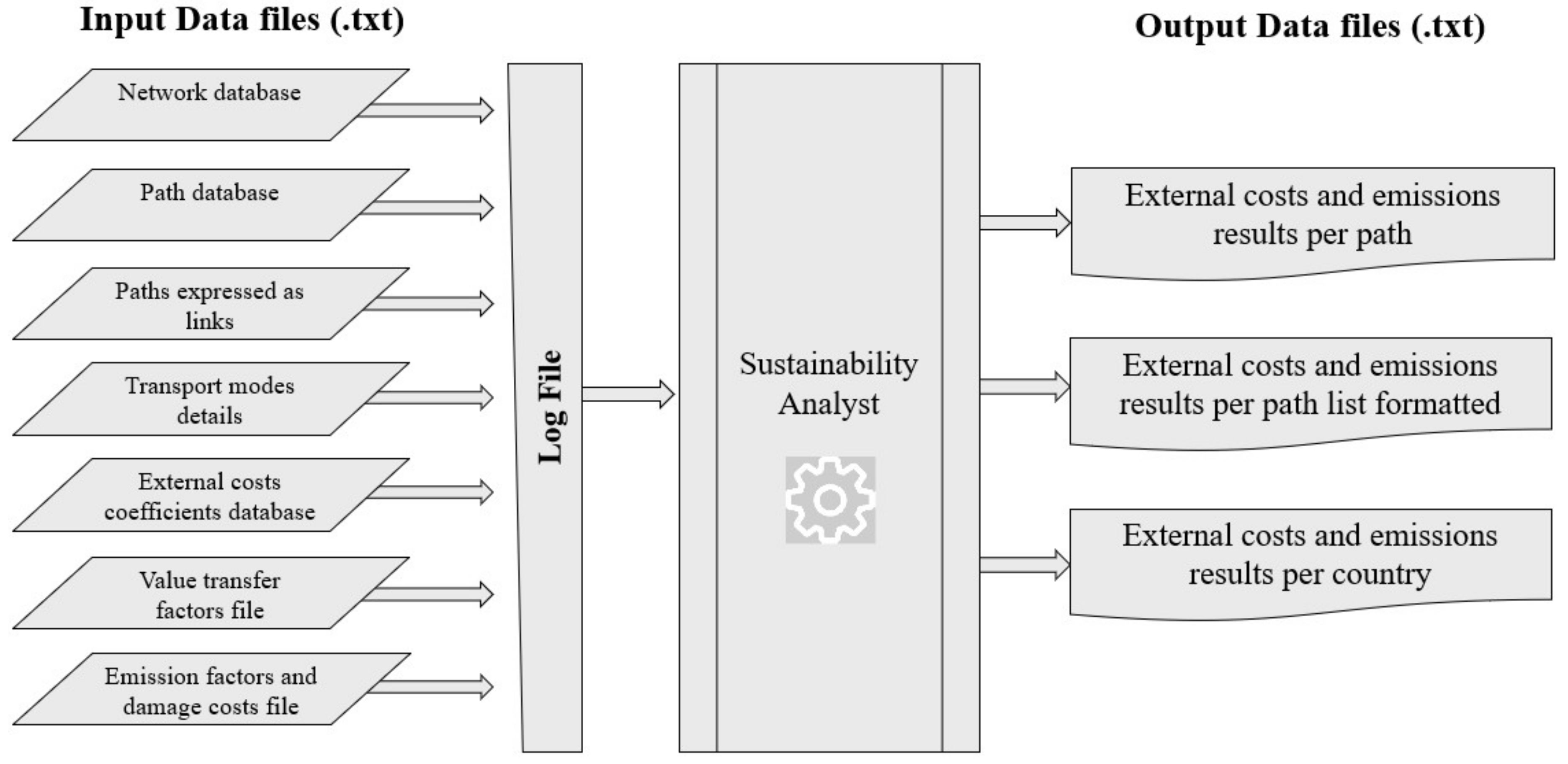
Finally, this methodology for calculating external costs (numerical model) has been implemented in a computational tool called Sustainability Analyst (SA), whose data flowchart is included in Figure 1.
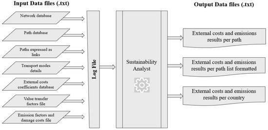
Figure 1.
Data flowchart of the software Sustainability Analyst.
4. Numerical Application
4.1. Case Study Definition
A case study for a corridor between the north of Portugal (Porto) and Germany (Stuttgart) using different alternative intermodal transport chains will be presented and numerical results for all external cost types associated with those chains will be compared. This corridor has been studied before [14] and its interest remains as there are significant volumes of trade between the Iberian Peninsula and the central European countries and the peripheral location of those countries can easily drive the modal shift from road to sea. Detailed results for emissions using these transport chains have been published before [15].
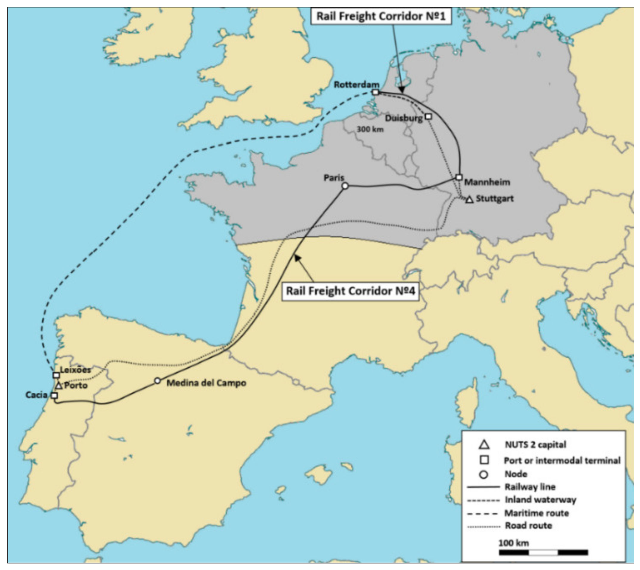
Table 3 describes the transport chains in terms of the transport modes involved, distances travelled and average speeds. The corresponding routes are schematically represented in Figure 2. All links part of a transport chain have an assigned average speed, which, for road links, is dependent on the type of road and level of congestion. For rail and maritime, the speed is specified at lower values when trains and ships move through links located close to rail terminals and ports. In all links speed is specified with values considered typical of the specific mode of transportation. Speed is adjustable link by link and values are stored in a database. It is also important to note that all trips are considered to take place during the day.
Table 3.
General characteristics of the different transport chains (A: unimodal; B–E: intermodal) between Porto and Stuttgart.

Figure 2.
Road, rail, IWW and maritime routes used in transport chains between Porto and Stuttgart.
The technical details of the vehicles used in these transport chains are adjustable, but in the case of this study they are as follows. For the road links, a 5 axle, 40 t EURO IV articulated truck is considered, having an engine power of 365 kW and a specific fuel oil consumption of 227 g/kWh. For the rail links, a long-haul diesel locomotive with a fuel consumption of 219 kg of fuel per hour, with a capacity fully utilized of 40 FEUs. A vessel with a full cargo capacity of 50 FEUs is considered for the inland waterways’ links, installed with a medium-speed diesel engine with 737 kW, diesel particulate filter and selective catalytic reduction for NOx emissions. A Ro-Ro cargo ship is considered for maritime links (main dimensions: Lbp = 180 m, B = 27 m, T = 7.5 m) having a deadweight of 13,535 t, a capacity of 239 trailers fully loaded, equipped with a medium-speed diesel engine with 12,000 kW, using VLSFO (0.5%S) outside the emission control area (ECA) in the North Sea and 0.1%S fuel inside the ECA, and 1270 kW of auxiliary power. The average time spent in each (origin and destination) port, when applicable, is 6 h. In the port the main engine is switched off but the auxiliary engines are kept running at 40% load [15].
4.2. Numerical Results for an Origin/Destination Pair
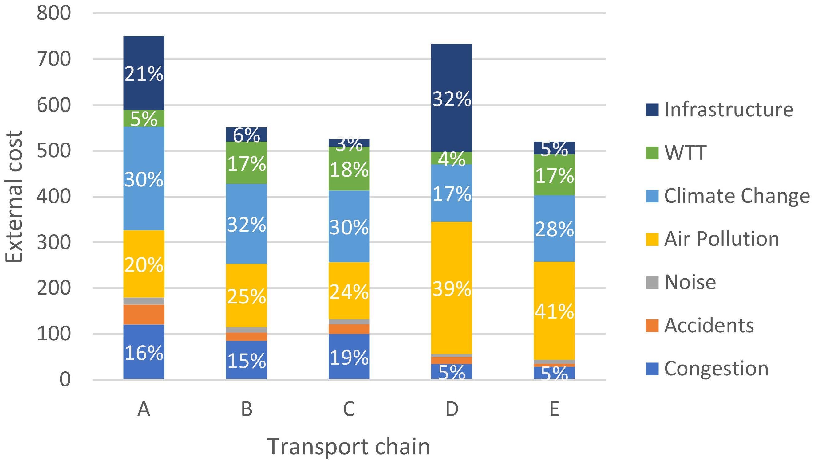
Figure 3 shows the values of each external cost type in the total external costs calculated for each transport chain per trailer. The most favourable alternative for this corridor, in terms of external costs, seems to be the intermodal SSS-based route E through Rotterdam and making use of a freight train to Manheim, followed closely by the other two SSS-based intermodal alternatives B and C. The intermodal rail-based alternative D sees its competitiveness reduced by the large external costs associated with air pollutant emissions associated with the use of a diesel locomotive for which emission standards are lower when compared to other inland modes [15]. The diesel freight train is the current solution used in the railway connection between the Iberian Peninsula and the other EU countries. On top of that, diesel trains have higher marginal infrastructure costs in France when compared with trucks [30]. France is also the country where the largest distance is travelled in both routes A and D, hence the larger infrastructure costs in the rail-based intermodal chain D when compared with the unimodal solution A. In general, the emission-related external costs are responsible for at least 50% of the total external cost figures in all alternative transport chains in this corridor. Higher well-to-tank emissions costs are related to the sea leg in chains B, C and E, sometimes with more than double the marginal cost factors for that mode than for the other modes. However, those factors are only available for selected cases in the Handbook, which do not specifically include the vessel type here considered. Congestion costs also register some relevance, being more than 15% of total external costs for the alternatives when larger distances are travelled by road but especially when those distances include the highly congested areas around the ports of Leixões and Rotterdam (chains B and C) and the peripheral highways of Paris (chain A). The congestion level of those roads is, as mentioned before, included in the network and its influence is also present in the calculation of air pollution and climate change costs.
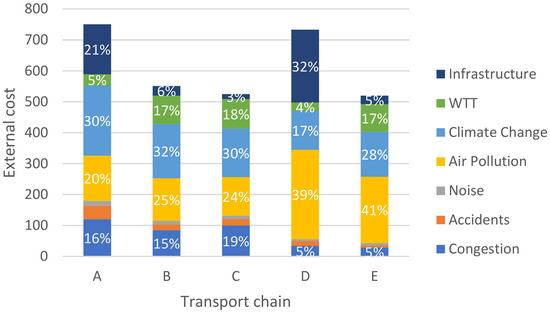
Figure 3.
External costs (€) per cost type in the transport chains between Porto and Stuttgart.
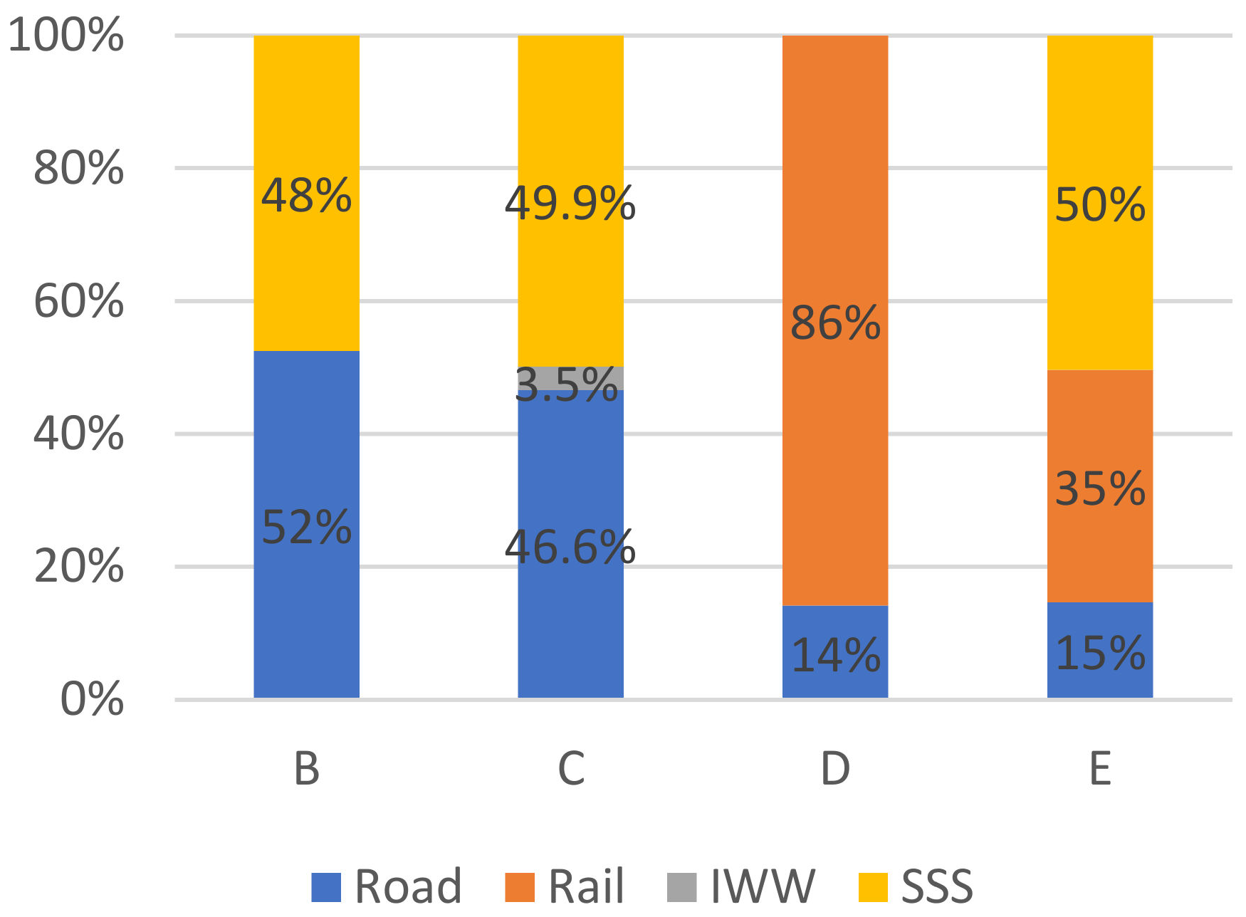
For the intermodal chains B–E, Figure 4 shows the share of each transport mode responsible for the external costs. While the share of external costs is proportional to the distance travelled by each mode, it becomes clear that the road legs of all the alternatives are more expensive per unit distance travelled than the legs travelled using other modes in these alternative chains. For example, in chains B and C, the road leg is responsible for around 50% of the external costs while corresponding to only 29% and 19% of the distance travelled, respectively. On the other hand, transport chains B, C and E, with the sea leg being more than 70% of the total distance travelled, is only responsible for around 50% of the total external costs in those chains. Finally, in transport chain D, rail represents 91% of the total travelled distance and this leads it to represent 86% of the external costs.
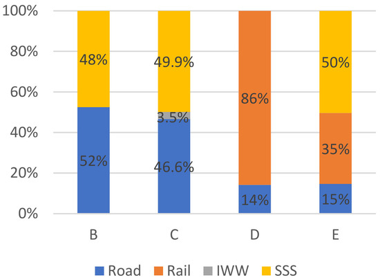
Figure 4.
Share of external cost per transport mode in the intermodal chains between Porto and Stuttgart.
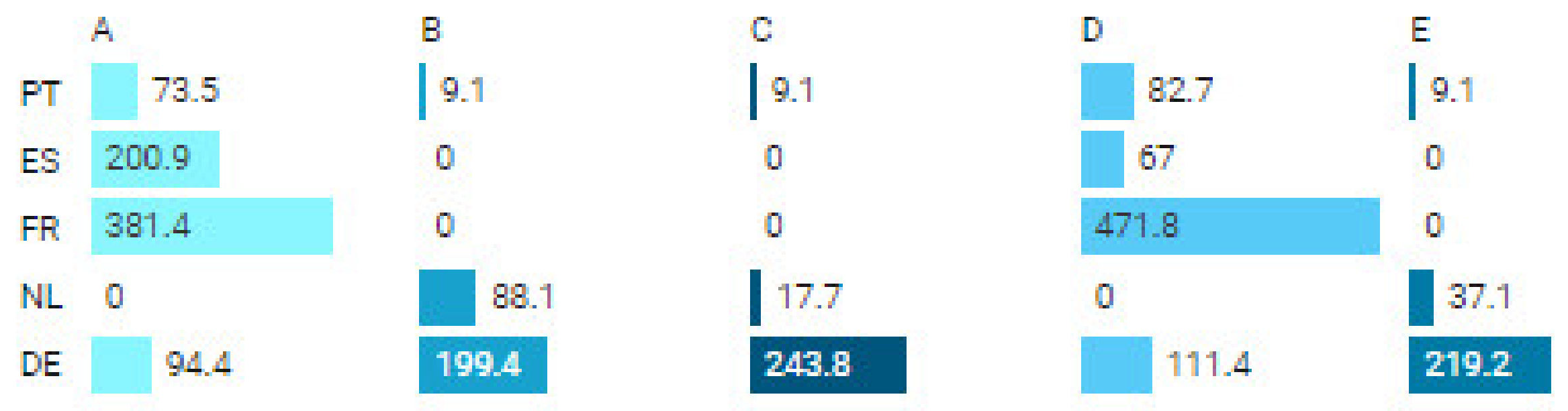
The numerical results on external costs may also be extracted per country for each transport chain. Figure 5 shows that in transport chain A and D most costs occur in France, where the travelled distances are larger (by road and rail, respectively).

Figure 5.
External costs (€) per country in the intermodal chains between Porto and Stuttgart.
4.3. Numerical Results for Multiple Origin/Destination Pairs
The numerical model presented above allows for the simultaneous study of multiple O/D pairs (each origin and destination representing a NUTS2 region). In this section, the numerical results will be presented for 75 destinations corresponding to NUTS 2 capitals covering a wide region, including a large part of northern France, Belgium, the Netherlands, Luxembourg and Germany. This geographical region was chosen as it comprises large areas and nations of considerable importance in terms of Portuguese foreign trade. Table S1 (Supplementary Materials) shows the numerical results for a number of key destinations spread across the area under study. The results in Table S1 comprise internal and external costs, in the latter case decoupled per mode of transportation, as well as the fraction of such costs that needs to be internalized. For each destination, the results are shown for the five transport chains under study (A–E).
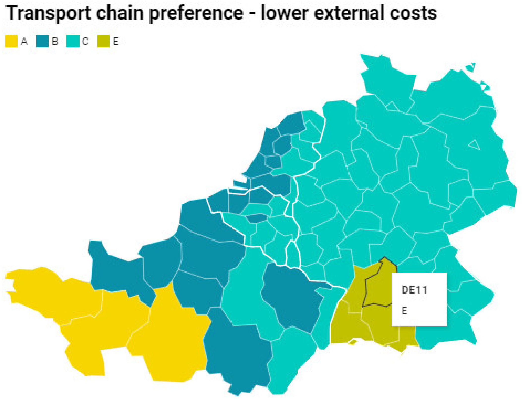
The results will be shown under the form of maps, such as that shown in Figure 6. The destination studied in detail in the previous section, Stuttgart, is shown in this map as region DE11. Most of the NUTS 2 regions show preference for intermodal SSS-based transport chains in terms of external costs. This means that those routes are the ones that would cause fewer impacts on society and the environment if chosen by transportation companies. The regions still attracted (mostly in Western France) by the unimodal transport chain A are the ones for which there is no efficient rail or IWW connection from the port of Rotterdam and so the road leg becomes largely responsible for the higher cost of the intermodal alternatives. The regions attracted the intermodal chain E fall close to the rail terminal in Manheim.

Figure 6.
Transport chain preference when considering as a criterion the lowest external cost (created with Datawrapper).
The isolated regions showing preference for chain B occur because of the slight differences in road lengths in the transport network model since the total costs in both alternatives B and C are very similar, as they were for the first O/D Porto–Stuttgart. Finally, the main conclusion of this figure is that transport chain B presents the lowest external costs mainly for a narrow fringe of coastal areas. However, for most of the NUTS 2 regions further inland, transport chain C (short sea shipping plus inland waterways) is the one with the lowest external costs. Transport chain D is not preferred by any NUTS 2 region due to the poor environmental performance of diesel trains.
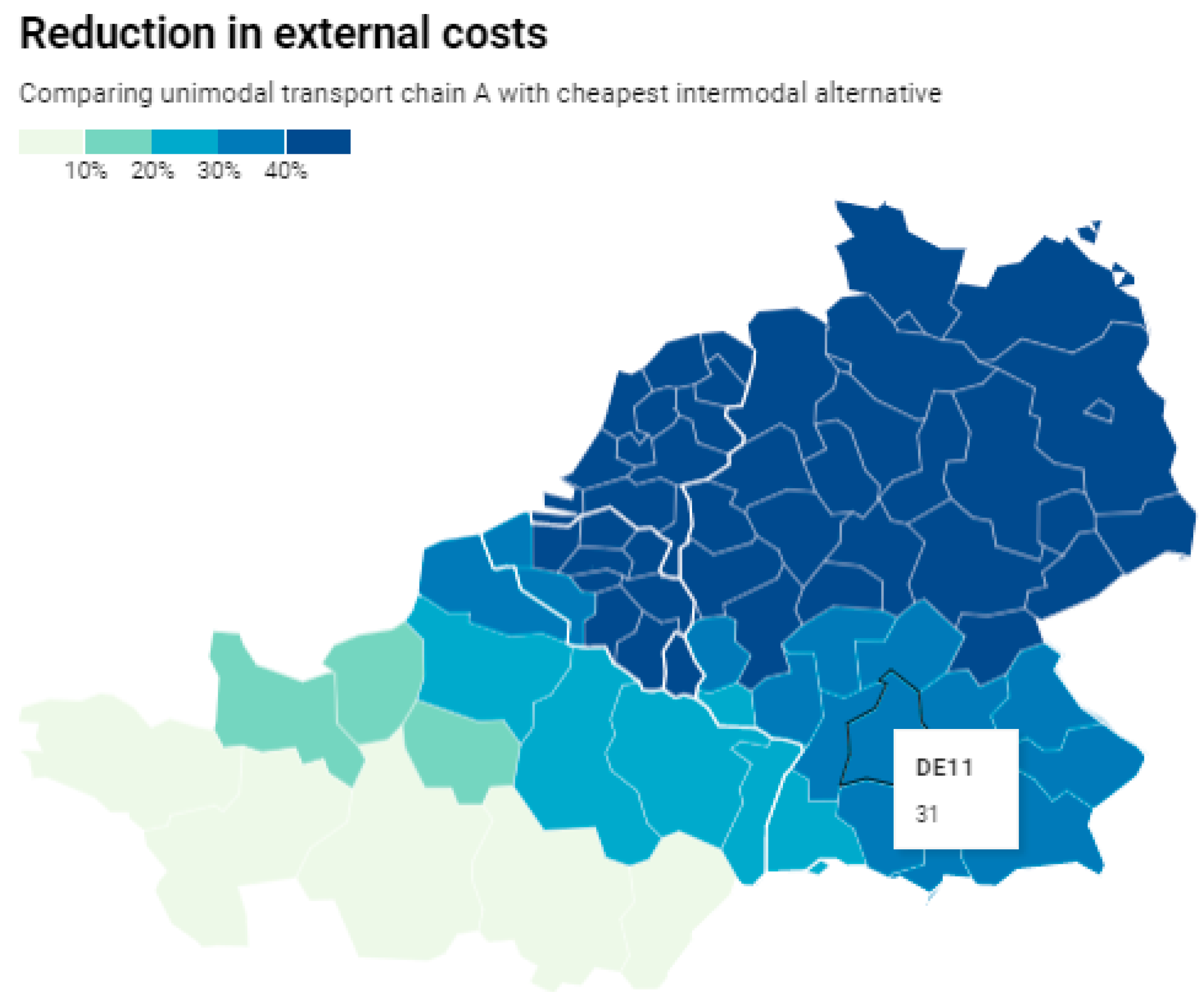
A further analysis may be done by directly comparing the intermodal solutions with road-based chain A. For this purpose, Figure 7 represents the reduction in external costs caused by a potential modal shift. The total costs of the unimodal solution A are compared with the computed cheapest intermodal alternative B–E in terms of total external costs. The main conclusions are that there are potential cost savings of more than 30% for most NUTS 2 regions across Germany, Netherlands and Belgium when an intermodal transport chain is chosen instead of the unimodal solution. Savings in external costs are also significant in northern France, although lower than in Germany. Given an assumed annual trailer number of 25,000 trailers, calculated for the one-way trip of the Ro-Ro two times a week between Porto and Stuttgart, the results mean that using intermodal solutions could save more than 5 million euros per year in external costs.

Figure 7.
Reduction in external costs when using intermodal transport solutions (created with Datawrapper).
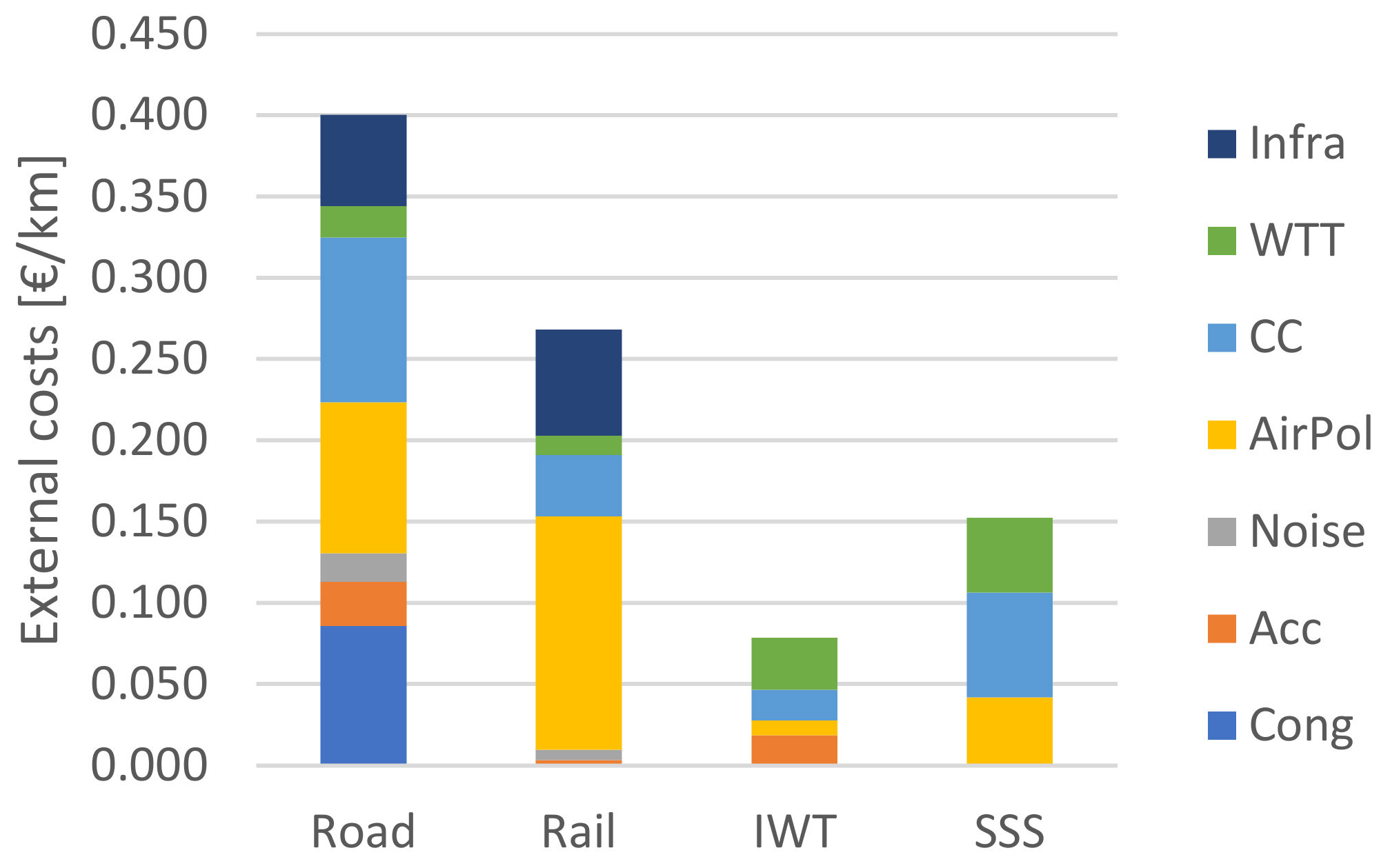
Figure 8 shows the most prevalent external cost types for each mode of transportation and for the average of such costs per distance travelled across all transport chains for the 75 destinations. It can be seen that for roads climate change and air pollution costs dominate, but congestion costs are also important. For rail, air pollution is the most important external cost. For SSS, external costs are dominated by climate change and air pollution costs, while IWW is dominated by well-to-tank costs. Finally, it can be seen that SSS and IWW present much lower total external costs per km than road or rail modes.

Figure 8.
External cost types most prevalent for each mode of transportation.
However, the choice between transportation chains cannot be made without considering also the internal costs associated with those chains. On average, considering all the chains included in this regional study, the external costs to internal costs ratio is only around 30%. The current degree of internalization must be considered so that the external costs (or parts of those) are not counted twice on the overall cost structure. The average cost coverage used for all EU countries is [11], as mentioned before, 62% for diesel trains, 37% for electric trains, 33% for trucks, 13% for IWW and 4% for maritime transport.
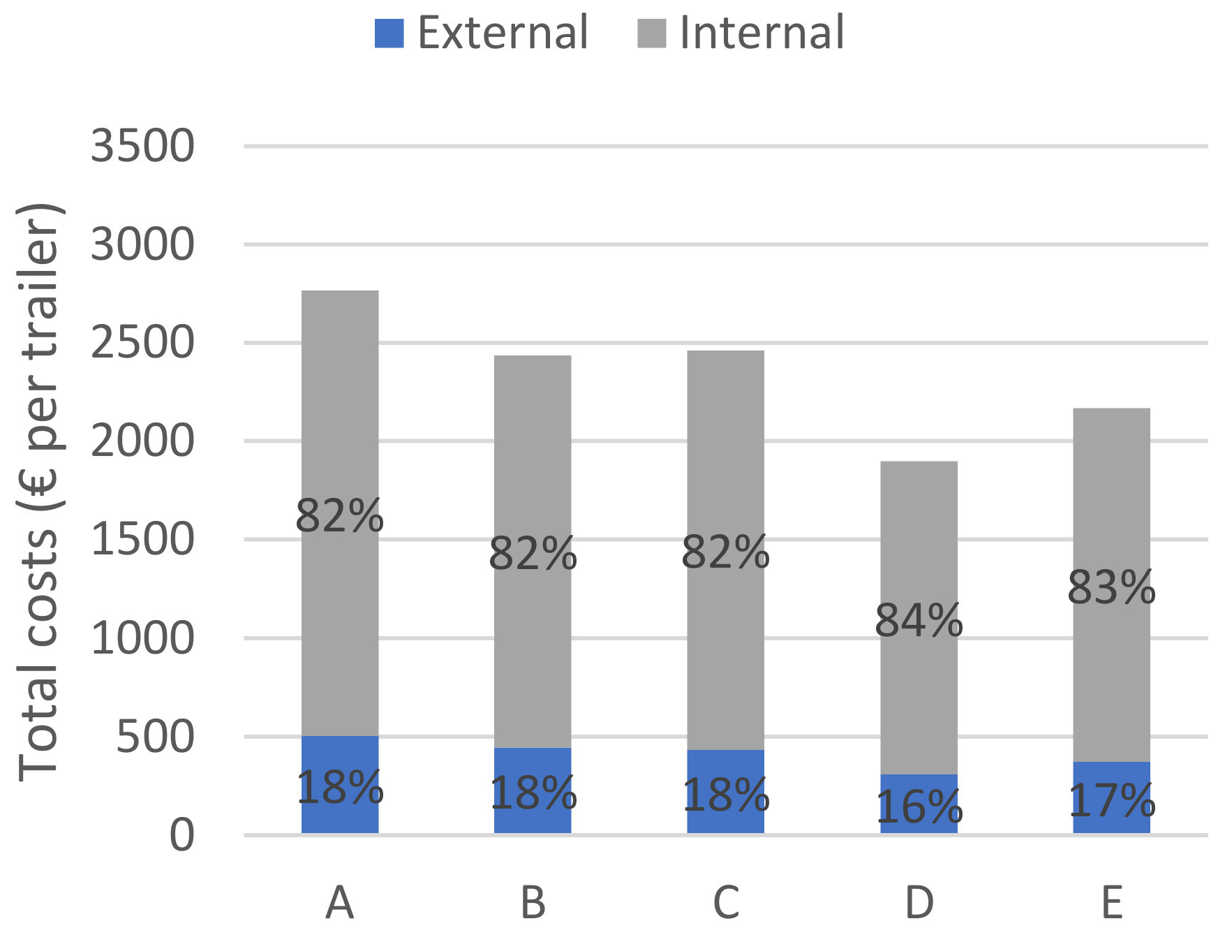
Figure 9 shows, for the first O/D Porto–Stuttgart, the total costs of transport taking the current internalization state into account. For this O/D pair, external costs consistently represent only close to 20% of the total costs of transport in each alternative chain. The competitiveness of the intermodal solutions is not significantly impacted by external costs and intermodal chains are still cheaper per unit of cargo, especially the rail-based solution D and the SSS-based solution E, and can represent large savings considering the potential volume of cargo to be transported per year. However, it is important to have in mind that this figure relates only to a specific pair origin/destination.

Figure 9.
Total costs per trailer comparison for the alternative transport chains between Porto and Stuttgart, taking the current internalization state into account.
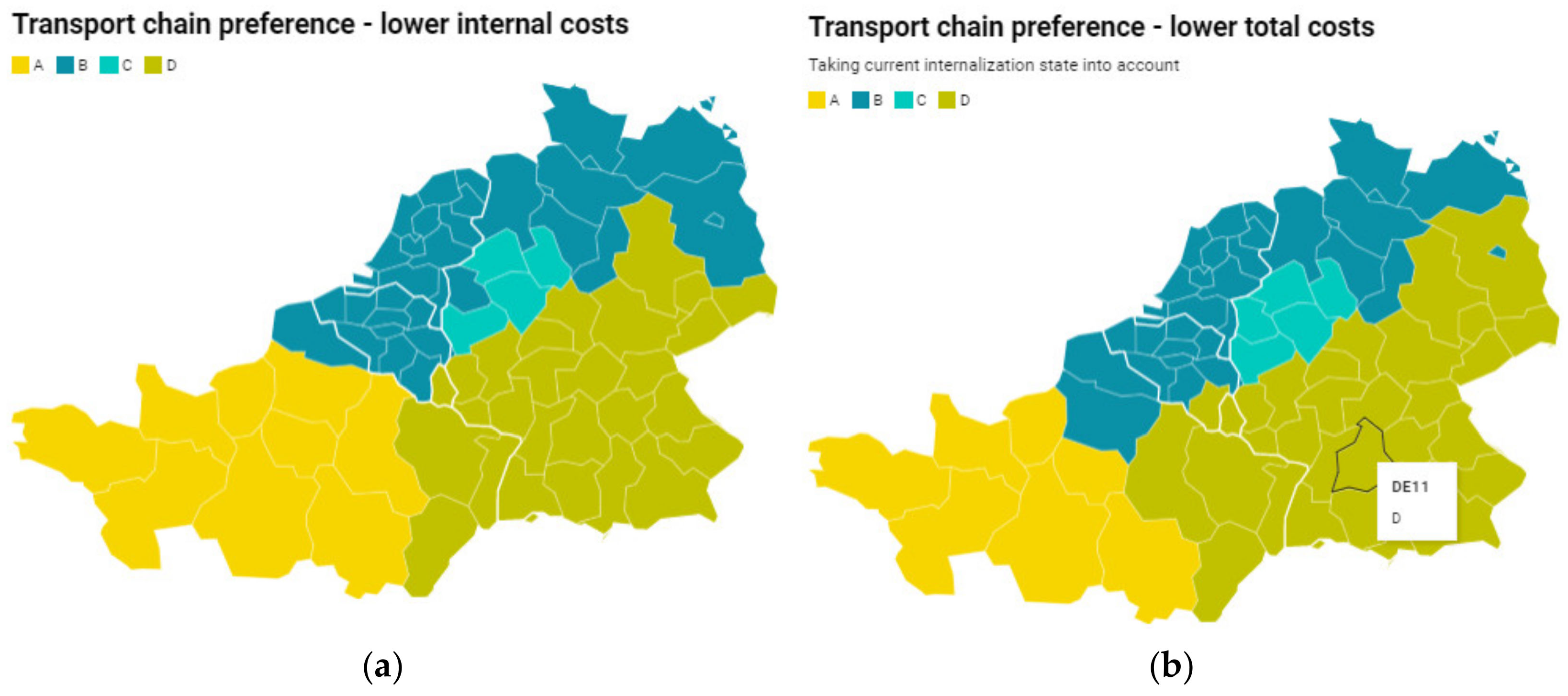
Figure 10 shows the preferred chains for all the 75 origin/destination pairs when only internal costs are considered (left) and when total costs are considered (thus including external costs, added to the extent that they are not already internalized). The main conclusion is that external costs, when added to the internal costs of transport in this corridor, promote the change to intermodal options in a few regions that, based only on internal cost prices, would prefer the road alternative. This is evident across northern and eastern France. Transport chain D is the main one responsible for such gains, but it is also possible to note that this chain also gains two regions from SSS, in East Germany and in East Belgium.

Figure 10.
Transport chain preference: (a) for lower internal costs; (b) for lower total costs taking the current internalization state into account (created with Datawrapper).
However, since the current internalization state for each mode can vary significantly between countries and is not sufficiently well documented in the literature, it is interesting to evaluate its effect on chain preference. Figure 11 shows the preference at the NUTS2 level based on total costs, neglecting that some part of the external costs may already be internalized, i.e., summing up 100% of the external costs with the internal costs. The main difference here is that the rail-based alternative D is now not competitive for any region and is surpassed by the three SSS-based solutions available (B, C and E). It is possible to see that transport chains C and E are the preferable chains across central and southern Germany. Chain B also becomes the preferred one for some more NUTS 2 regions in northern France. Clearly, the high external costs of rail in transport chain D (because of the diesel train) penalize strongly its competitiveness when the external costs are added in full to the internal costs, and the existing degree of internalization is an important aspect to be taken into account.
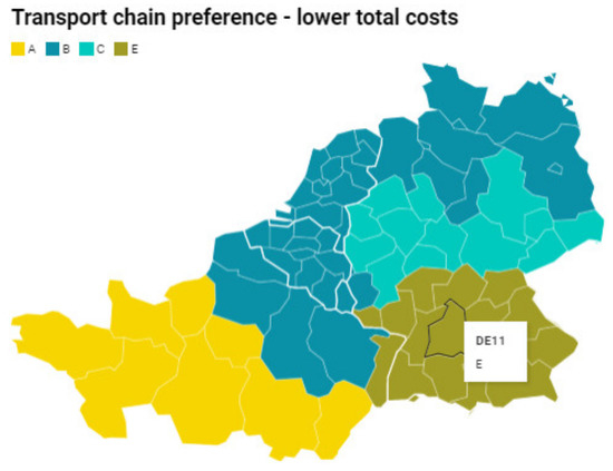
Figure 11.
Transport chain preference for lower total costs, not taking the current internalisation state into account (created with Datawrapper).
5. Conclusions
This paper has presented and applied a methodology to calculate the external costs of transportation in complex intermodal transportation chains that include several transport modes. A computational tool that implements this methodology was developed and is used in this paper in a numerical study dedicated to the evaluation of the competitiveness of short sea shipping-based intermodal chains when compared to road- and rail-based chains. This study relates to the Atlantic Corridor, namely, between the north-western part of the Iberian Peninsula and northern continental Europe (Netherland, Belgium, Germany and northern France). This paper adds to the literature by providing detailed numerical results for the individual intermodal transport chains running between different origin/destination pairs across this wide area. The results cover the external costs, decoupled per transport mode, for each alternative transport chain, but may also be decoupled per country. These results make it possible to assess the magnitude of the external costs for different transport chains and the relative importance of the different components of the external costs for each specific origin/destination pair.
This paper also contributes to the literature dealing with the external costs of transportation through the identification of geographical areas (groups of NUTS 2 regions) where a certain transport chain is more competitive in terms of internal cost, external cost or total cost. It was concluded that transport chains that include SSS to Rotterdam (coupled to road, IWW or rail) present lower external costs than road haulage or rail (with diesel-powered vehicles) from Portugal. Another contribution is the conclusion that the external costs of SSS-based chains are 30 to 40% lower than the external costs of road haulage direct from Portugal, for the NUTS 2 regions beyond France. Therefore, regarding external costs, SSS-based intermodal chains are preferable for most of the geographical area under study.
This paper also contributes through the conclusion that external costs, calculated for the O/D pairs in this corridor using the values provided in the EU handbook, amount to only about 20–30% of the internal costs for most origin/destination pairs. When added to the internal costs, taking into consideration the existing degree of internalization of external costs in the EU, they do not change significantly the geographical scope of competitiveness of the SSS-based chains. In general, SSS is more competitive in total cost up to about 300 km from the coastline, but some NUTS 2 regions in East Germany, East France and Belgium are gained for railway and others in Northern France are gained for SSS, when external costs are added. Inwards of about 300 km from the coast, the rail-based chain is the most competitive, even though it is based on diesel trains. In this corridor, the external cost coefficients and carbon price would need to be higher if the balance between road and intermodal transport is to be significantly tipped in favour of the latter.
A final contribution of this paper is the identification, from a geographical point of view, of the impact that the current degree of internalization of external costs (differentiated for the various modes of transportation) has in the delimitation of SSS competitiveness areas. In fact, SSS-based chains (especially that using also the railway from Rotterdam to Mannheim) fully replace the rail chain from Portugal, for most of southern Germany. Therefore, it is clear that the existing degree of internalization needs to be accounted for in the study of the competitiveness of alternative transport chains, as it has been shown to have a significant effect on the relative competitiveness of transport chains.
Several aspects in the calculation of external costs need to be considered in detail during further research, namely, the variation in the degree of internalization between different EU countries and the influence on the geographical areas where different transport chains are more competitive regarding the type of fuels used by the vehicles and, especially, those used by ships. The utilization of alternative fuels, such as LNG, methanol or even 0.1% sulphur-content fuels (all along the maritime route), will decrease climate change, air pollution and the well-to-tank cost components, and, therefore, are likely to increase the area for which SSS is more competitive.
Supplementary Materials
The following are available online at https://www.mdpi.com/article/10.3390/jmse9090959/s1, Table S1: External costs per mode of transportation, total external costs and fraction requiring internalisation.
Author Contributions
Conceptualization, M.M.R. and T.A.S.; methodology, M.M.R.; software and validation, M.M.R.; formal analysis, T.A.S.; investigation and resources, M.M.R. and T.A.S.; data curation, M.M.R.; writing—original draft preparation, M.M.R.; writing—review and editing, T.A.S.; visualization, M.M.R.; supervision, T.A.S.; project administration, T.A.S.; funding acquisition, T.A.S. All authors have read and agreed to the published version of the manuscript.
Funding
This research was funded by Fundação para a Ciência e a Tecnologia (FCT), grant number PTDC/ECI-TRA/28754/2017 and contributes to the Strategic Research Plan of the Centre for Marine Technology and Ocean Engineering (CENTEC), which is financed by FCT under contract UIDB/UIDP/00134/2020.
Institutional Review Board Statement
Not applicable.
Informed Consent Statement
Not applicable.
Data Availability Statement
The data presented in this study are available on request from the corresponding author.
Acknowledgments
The research presented in this paper was conducted within the research project “Evaluation of short sea shipping services integrated in supply chains”, financed by the Portuguese Foundation for Science and Technology (Fundação para a Ciência e Tecnologia-FCT), under contract PTDC/ECI-TRA/28754/2017. This work contributes to the Strategic Research Plan of the Centre for Marine Technology and Ocean Engineering (CENTEC), which is financed by FCT under contract UIDB/UIDP/00134/2020.
Conflicts of Interest
The authors declare no conflict of interest. The funders had no role in the design of the study; in the collection, analyses, or interpretation of data; in the writing of the manuscript, or in the decision to publish the results.
References
- European Commission. Roadmap to a Single European Transport Area—Towards a Competitive and Resource Efficient Transport System; European Commission: Brussels, Belgium, 2011. [Google Scholar]
- European Commission; Secretariat-General. The European Green Deal; European Commission: Brussels, Belgium, 2019. [Google Scholar]
- European Commission; Directorate-General for Mobility and Transport. Sustainable and Smart Mobility Strategy—Putting European Transport on Track for the Future; COM/2020/789 Final; European Commission: Brussels, Belgium, 2020. [Google Scholar]
- Community of European Railway and Infrastructure Companies. Position Paper, Implementing User-Pays and Polluter-Pays in Road Charging: CER’s Proposals for Council Discussions on Eurovignette; CER: Brussels, Belgium, 2019. [Google Scholar]
- Electro-Mobility Platform. Position on the Proposal of 31 May 2017 by the European Commission for a Revised ‘Eurovignette’ Directive (1999/62/EC) on Road Charging. Available online: https://www.platformelectromobility.eu/wp-content/uploads/2018/02/E-Mobility-Platform-Eurovignette-paper-for-Council-18-March-2019.pdf (accessed on 18 March 2019).
- Community of European Railway and Infrastructure Companies. Position Paper, Europe’s Economic Recovery after Covid-19: Help Finance It by Applying User-Pays and Polluter-Pays Principles in Transport; European Commission: Brussels, Belgium, 2020. [Google Scholar]
- van Essen, H.; van Wijngaarden, L.; Schroten, A.; Sutter, D.; Bieler, C.; Maffii, S.; Brambilla, M.; Fiorello, D.; Fermi, F.; Parolin, R.; et al. Handbook on the External Costs of Transport Version 2019—1.1; CE Delft: Delft, The Netherlands, 2019. [Google Scholar]
- Sambracos, E.; Maniati, M. Competitiveness between short sea shipping and road freight transport in mainland port connections; the case of two Greek ports. Marit. Policy Manag. 2012, 39, 321–337. [Google Scholar] [CrossRef]
- Tzannatos, E.; Papadimitriou, S.; Katsouli, A. The cost of modal shift: A short sea shipping service compared to its road alternative in Greece. Eur. Transp. Trasp. Eur. 2014, (56), Paper Nº2. 1–20. [Google Scholar]
- Hofbauer, F.; Putz, L.-M. External Costs in Inland Waterway Transport: An Analysis of External Cost Categories and Calculation Methods. Sustainability 2020, 12, 5874. [Google Scholar] [CrossRef]
- Raza, Z.; Svanberg, M.; Wiegmans, B. Modal shift from road haulage to short sea shipping: A systematic literature review and research directions. Transp. Rev. 2020, 40, 382–406. [Google Scholar] [CrossRef] [Green Version]
- van Essen, H.; van Wijngaarden, L.; Schroten, A.; Sutter, D.; Schmidt, M.; Brambilla, M.; Maffii, S.; El Beyrouty, K.; Morgan-Price, S.; Andrew, E. State of Play of Internalisation in the European Transport Sector; CE Delft: Delft, The Netherlands, 2019. [Google Scholar]
- Ramalho, M.; Santos, T.; Soares, C.G. External costs in short sea shipping based intermodal transport chains. In Developments in Maritime Technology and Engineering; Santos, T.A., Guedes Soares, C., Eds.; Routledge, Taylor & Francis Group: London, UK, 2020; pp. 63–72. [Google Scholar]
- Santos, T.A.; Ramalho, M.M.; Guedes Soares, C. Sustainability in short sea shipping-based intermodal transport chains. In Short Sea Shipping in the Age of Sustainable Development and Information Technology; Santos, T.A., Guedes Soares, C., Eds.; Routledge: London, UK, 2020; pp. 89–115. [Google Scholar]
- Ramalho, M.M.; Santos, T.A. Numerical modelling of air pollutants and greenhouse gases emissions in intermodal transport chains. J. Mar. Sci. Eng. 2021, 9, 679. [Google Scholar] [CrossRef]
- Vierth, I.; Sowa, V.; Cullinane, K. Evaluating the external costs of trailer transport: A comparison of sea and road. Marit. Econ. Logist. 2019, 21, 61–78. [Google Scholar] [CrossRef]
- Ricardo-AEA, TRT, DIW Econ & CAU. Update of the Handbook on External Costs of Transport; Ricardo-AEA: London, UK, 2014. [Google Scholar]
- Pigou, A.C. The Economics of Welfare; Palgrave classics in economics; Palgrave Macmillan: London, UK, 1920. [Google Scholar]
- World Bank. State and Trends of Carbon Pricing 2020; World Bank: Washington, DC, USA, 2020. [Google Scholar]
- Chatziioannou, I.; Alvarez-Icaza, L.; Bakogiannis, E.; Kyriakidis, C.; Chias-Becerril, L. A Structural Analysis for the Categorization of the Negative Externalities of Transport and the Hierarchical Organization of Sustainable Mobility’s Strategies. Sustainability 2020, 12, 6011. [Google Scholar] [CrossRef]
- Progiou, A.G.; Bakeas, E.; Evangelidou, E.; Kontogiorgi, C.; Lagkadinou, E.; Sebos, I. Air pollutant emissions from Piraeus port: External costs and air quality levels. Transp. Res. Part D 2021, 91, 102586. [Google Scholar] [CrossRef]
- Hintjens, J.; van Hassel, E.; Vanelslander, T.; Van de Voorde, E. Port Cooperation and Bundling: A Way to Reduce the External Costs of Hinterland Transport. Sustainability 2020, 12, 9983. [Google Scholar] [CrossRef]
- Janic, M. Modelling the full costs of an intermodal and road freight transport network. Transp. Res. Part D Transp. Environ. 2007, 12, 33–44. [Google Scholar] [CrossRef]
- Comi, A.; Polimeni, A. Assessing the Potential of Short Sea Shipping and the Benefits in Terms of External Costs: Application to the Mediterranean Basin. Sustainability 2020, 12, 5383. [Google Scholar] [CrossRef]
- Ambrosino, D.; Ferrari, C.; Sciomachen, A.; Tei, A. Intermodal nodes and external costs: Re-thinking the current network organization. Res. Transp. Bus. Manag. 2016, 19, 106–117. [Google Scholar] [CrossRef] [Green Version]
- Ambrosino, D.; Sciomachen, A.; Surace, C. Evaluation of flow dependent external costs in freight logistics networks. Networks 2019, 74(2), 111–123. [Google Scholar] [CrossRef]
- European Parliament; Council of the European Union. Directive 2011/76/EU of 27 September 2011 amending Directive 1999/62/EC on the charging of heavy goods vehicles for the use of certain infrastructures. Off. J. Eur. Union 2011, L269, 1–16. [Google Scholar]
- Schroten, A.; van Essen, H.; van Wijngaarden, L.; Sutter, D.; Andrew, E. Sustainable Transport Infrastructure Charging and Internalisation of Transport Externalities; Report for Directorate-General for Mobility and Transport; European Commission: Brussels, Belgium, 2019. [Google Scholar]
- Vierth, I.; Merkel, A. Internalization of external and infrastructure costs related to maritime transport in Sweden. Res. Transp. Bus. Manag. 2020, 100580. [Google Scholar] [CrossRef]
- Schroten, L.; van Wijngaarden, M.; Brambilla, M.; Gatto, S.; Maffii, F.; Trosky, H.; Kramer, R.; Monden, D.; Bertschmann, M.; Killer, V.; et al. Overview of Transport Infrastructure Expenditures and Costs; Report for Directorate-General for Mobility and Transport; European Commission: Brussels, Belgium, 2019. [Google Scholar]

Publisher’s Note: MDPI stays neutral with regard to jurisdictional claims in published maps and institutional affiliations. |
© 2021 by the authors. Licensee MDPI, Basel, Switzerland. This article is an open access article distributed under the terms and conditions of the Creative Commons Attribution (CC BY) license (https://creativecommons.org/licenses/by/4.0/).