A Finite Element Model for Underwater Sound Propagation in 2-D Environment

Abstract

The finite element method is a popular numerical method in engineering applications. However, there is not enough research about the finite element method in underwater sound propagation. The finite element method can achieve high accuracy and great universality. We aim to develop a three-dimensional finite element model focusing on underwater sound propagation. As the foundation of this research, we put forward a finite element model in the Cartesian coordinate system for a sound field in a two-dimensional environment. We firstly introduce the details of the implementation of the finite element model, as well as different methods to deal with boundary conditions and a comparison of these methods. Then, we use four-node quadrilateral elements to discretize the physical domain, and apply the perfectly matched layer approach to deal with the infinite region. After that, we apply the model to underwater sound propagation problems including the wedge-shaped waveguide benchmark problem and the problem where the bathymetry consists of a sloping region and a flat region. The results by the presented finite element model are in excellent agreement with analytical and benchmark numerical solutions, implying that the presented finite element model is able to solve complex two-dimensional underwater sound propagation problems accurately. In the end, we compare the finite element model with the popular normal mode model KRAKEN by calculating sound fields in Pekeris waveguides, and find that the finite element model has better universality than KRAKEN.

1. Introduction

There are a variety of methods for calculating the underwater sound fields, such as the ray method, the normal mode method, and the parabolic equation method. However, the finite element method is used by only a few researchers to solve underwater sound propagation problems.

As we all know, the finite element method is a universal numerical calculation method in many engineering fields. The basic principle of the finite element method is to discretize the continuous area into limited number of elements and nodes. We can use elements of different shapes to deal with the boundaries of complex shapes.

The finite element method was first put forward by Clough [1] in 1960 for a plane elasticity problem. Finite element methods for time–harmonic acoustics governed by the Helmholtz equation have been an active research area over the past 50 years. Initial applications of finite element methods for time–harmonic acoustics focused on interior problems with complex geometries including direct and modal coupling of structural acoustic systems for forced vibration analysis, frequency response of acoustic enclosures, and waveguides [2,3,4]. In recent years, tremendous progress has been made; for example, extending the finite element method to exterior problems in unbounded domains and higher frequency regimes, which incorporates knowledge of wave behavior into the algorithm, combined with parallel sparse interactive and domain decomposition solvers.

The exterior acoustics problem in unbounded domains presents a special challenge for finite element methods. In order to apply the FEM to exterior problems, the unbounded domain is usually truncated by an artificial boundary, yielding a bounded computational domain. The first complete finite element approach for modeling acoustic radiation and scattering in unbounded domains appears in the impedance matching technique presented by Hunt [5,6]. Recent numerical treatments including infinite elements, absorbing layers, local absorbing boundary conditions, and exact nonlocal boundary conditions have proven to be effective in handling acoustic scattering problems in unbounded domains, especially for large-scale problems requiring interactive and parallel solution methods and for modeling inhomogeneities and acoustic-structure interaction. The choice of methods depends on the shapes and complexity of the scattering objects, inhomogeneities, frequency range, and resolution requirements, among other parameters.

The infinite elements are constructed with radial wave functions that automatically satisfy the radiation boundary condition. Bettess [7] pioneered the infinite element concept and selected the test function to be the same as the trial solution basis. However, the performance of both conjugated and unconjugated formulations deteriorates at larger wavenumbers and highly elongated artificial interfaces [8]. The perfectly matched layer (PML) concept was originally introduced by Berenger [9,10] for electromagnetic waves. It is another option for modeling the far field for the exterior acoustics problem. The idea is to introduce an exterior layer of finite thickness at an artificial interface such that outgoing waves are absorbed prior to reaching the outer-layer truncation boundary. By splitting the scalar field into nonphysical components, satisfying equations that describe decaying waves and proper selection of PML coefficients, plane-wave reflection for an arbitrary angle of incidence is theoretically eliminated. There is also a great deal of research on absorbing boundary conditions [11] and the DtN nonreflecting boundary conditions [12,13].

The finite element method is able to solve problems in inhomogeneous media and allows for a natural coupling with complex structures. For exterior problems in unbounded domains, special techniques are required to reduce spurious reflection to a level below that of the discretization error. The numerical advantage of the FEM is that it leads to sparse matrices, which significantly speeds up computations and reduces memory requirements. Complexity estimates [14,15] show that domain-based methods such as the FEM are an effective alternative to the BEM for exterior acoustics problems, especially for large systems due to the sparse structure of the resulting system matrices. With the recent development in fast multiple methods, which accelerates the calculation of matrix-vector products in iterative integral methods [16], the method with the best efficiency is less clear, yet the FEM retains the advantages of robustness and natural integration with other discrete models in coupled problems. It is also possible to couple the finite method with boundary integral methods [17] and other domain-based methods, such as global Trefftz-based wave methods, which are effective at high frequencies on moderate geometrical complexity [18].

However, there is not such large amount of research on finite element methods in ocean acoustics. In the 1990s, Murphy and Chin-Bing [19,20,21] established a finite element model FOAM for shear waves in marine sediment. They put forward a wide-angle radiation condition, which is actually a kind of parabolic equation, to simulate the infinite area. In 1999, Kampanis and Dougalis [22] established a finite element model FENL in axially symmetric waveguides. They used the Dirichlet-to-Neumann boundary condition to simulate the infinite area. In 2006, Li Jun [23] established a finite element model FEMLJ for prediction of sound fields in shallow water, which used the same methods as those in FENL. In 2008, Athanassoulis [24] compared the finite element model FENL with coupled normal mode model CCMM. Then, in the next 10 years, more and more researchers began to focus on commercial finite element software for oceanographic phenomena and scattering problems [25,26]. In 2013, Goldsberry and Isakson [27] mentioned in their paper that performing a fully three-dimensional finite element model is currently unfeasible due to the difficulties in implementation and limits in computational power. They compared two promising methods to represent the 3D field, the longitudinally invariant (LI) method and a 2D axial-symmetric reduction of the 3D Helmholtz equation. They used these two methods for ASA benchmark problem, but failed to agree with the PE solution. From 2016 to 2020, Chai Yingbing [28,29,30] focused on solving the numerical dispersion problem for the high-frequency problem by the traditional finite element method and put forward several methods to soften the stiffness matrix.

As can be seen, there is not enough research on finite element modeling in underwater sound propagation. Most of the existing finite element models rely on commercial software or focus on reverberation problems rather than propagation problems. In this paper, we will propose a finite element model for underwater sound propagation in a two-dimensional environment. We will also introduce the implementation in detail and show the results of this model.

2. Practical Aspects of the Implementation

The basic idea of the finite element method is transforming an infinite dimensional problem into a finite dimensional problem, through discretizing the physical domain into several elements with finite number of nodes.

In this section, the specific steps of our finite element model will be described. Firstly, the weak form of the Helmholtz equation is derived through the traditional Galerkin method. Then, four-node quadrilateral elements are used to discretize the physical domain. We assemble all the local stiffness matrices into a global stiffness matrix. In the end, the treatment of boundaries is discussed.

2.1. Weak Form of Helmholtz Equation

This finite element model mainly focuses on calculation of the two-dimensional sound field in the Cartesian coordinate system at a specific frequency. So, the following discussion is based on the Helmholtz equation.

The Helmholtz equation [31] in an inhomogeneous medium without sources is

$$\nabla ·\left(\frac{1}{\rho (x,z)}\nabla p\right)+\frac{k^2(x,z)p}{\rho (x,z)}=0,(x,z)\in \Omega ,$$

(1)

where $\Omega$ is a bounded domain in the $(x,z)$ plane with the boundary $\partial \Omega$; p is a function of $(x,z)$ indicating the sound pressure; and $\rho$ and k are functions of $(x,z)$ indicating density and wave number, respectively.

Multiply both sides of Equation (1) with a test function $q(x,z)$ and obtain

$$\left[\nabla ·\left(\frac{1}{\rho (x,z)}\nabla p\right)+\frac{k^2(x,z)p}{\rho (x,z)}\right]q(x,z)=0.$$

(2)

Then, integrate the equation over $\Omega$,

$${\int \int }_{\Omega }\left[\nabla ·\left(\frac{1}{\rho (x,z)}\nabla p\right)+\frac{k^2(x,z)p}{\rho (x,z)}\right]q(x,z)\mathrm{d}x\mathrm{d}z=0.$$

(3)

Finally, apply the Gauss theorem to obtain the weak formation of the Helmholtz equation,

$${\int }_{\partial \Omega }\frac{q}{\rho }\frac{\partial p}{\partial \overrightarrow{n}}\mathrm{d}s-\underset{\Omega }{\int \int }\frac{1}{\rho }\nabla p·\nabla q\mathrm{d}x\mathrm{d}z+\underset{\Omega }{\int \int }\frac{1}{\rho }{k}^{2}pq\mathrm{d}x\mathrm{d}z=0,$$

(4)

where the first term indicates the integral on the boundary of $\Omega$, the second and third terms indicate the integral on $\Omega$. We will discuss the discretization of $\Omega$ and $\partial \Omega$ separately.

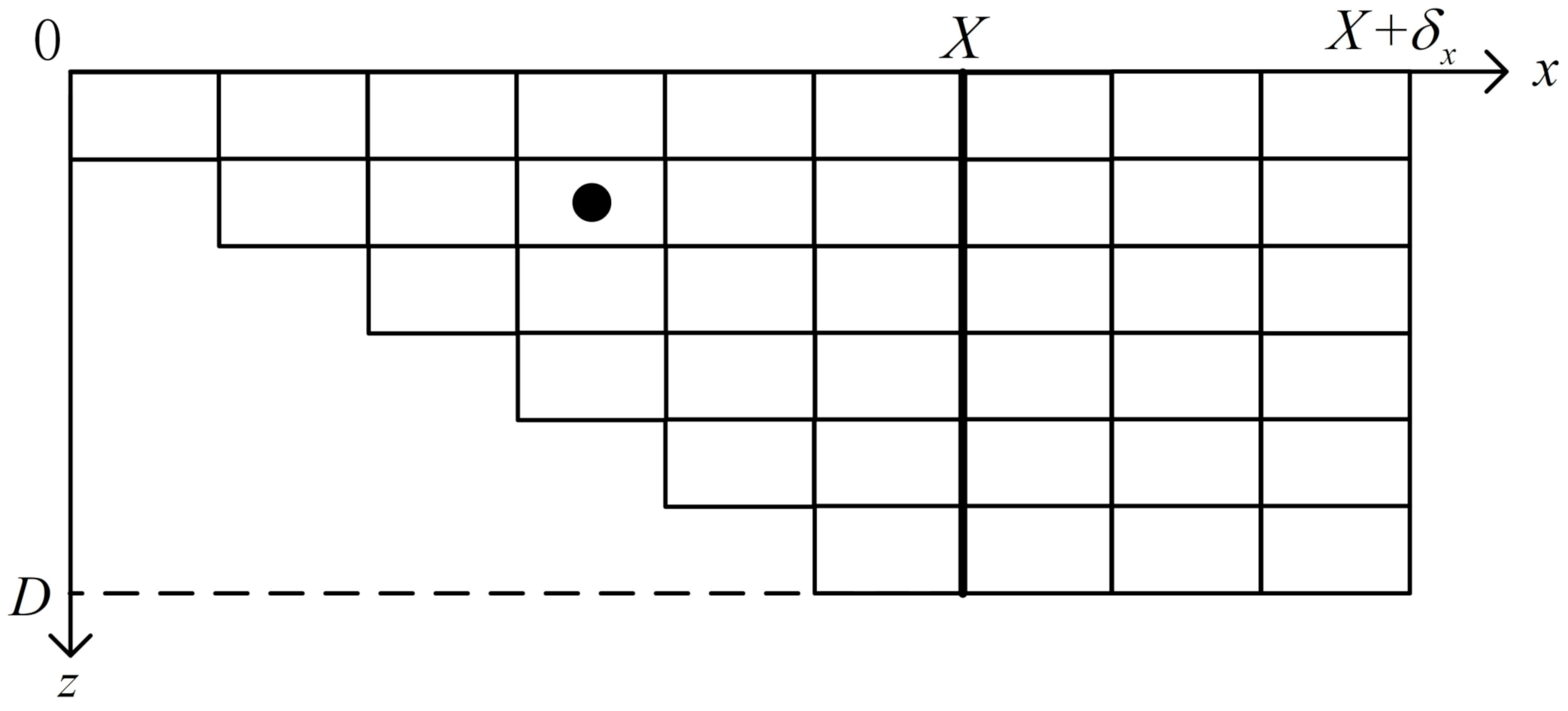
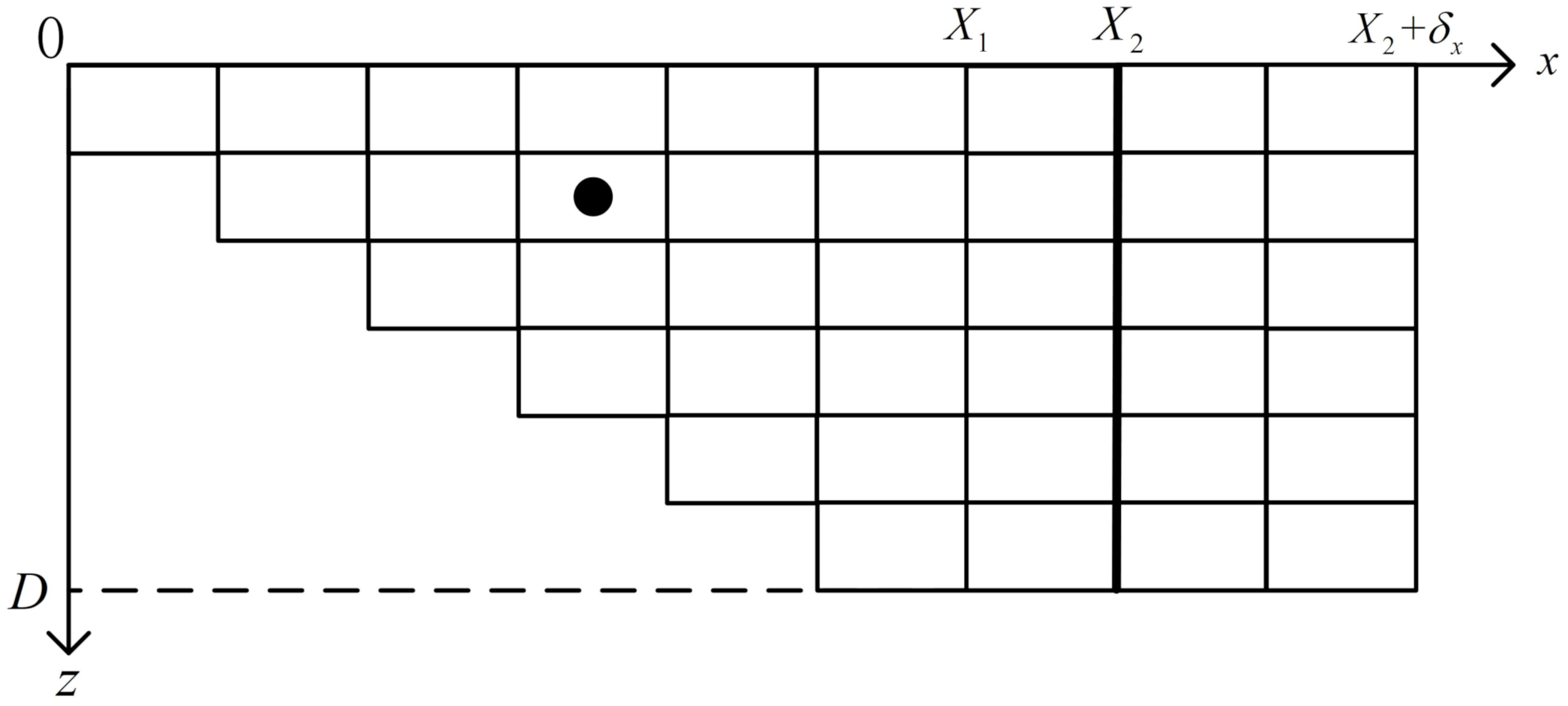
2.2. The Finite Element Discretization

In order to calculate the last two terms of Equation (4), we use four-node quadrilateral elements to discretize $\Omega$. Figure 1 is a schematic diagram of a four-node quadrilateral element and its local indices, midpoint coordinates $(x_0,z_0)$, length $2a$, and width $2b$. We define the element as ${\Omega }_{\mathrm{e}}$.

We use $N_n(x,z)$ for the shape functions or the basis functions, where $n=1,2,3,4$ indicates the local index of four nodes. $N_n(x,z)$ can be written as the following form using the Lagrange interpolation method,

$$\left\{\begin{array}{c}{\displaystyle N_1(x,z)=\frac{1}{4}\left({\displaystyle 1-\frac{x-x_0}{a}}\right)\left({\displaystyle 1-\frac{z-z_0}{b}}\right),}\hfill \\ {\displaystyle N_2(x,z)=\frac{1}{4}\left({\displaystyle 1+\frac{x-x_0}{a}}\right)\left({\displaystyle 1-\frac{z-z_0}{b}}\right),}\hfill \\ {\displaystyle N_3(x,z)=\frac{1}{4}\left({\displaystyle 1+\frac{x-x_0}{a}}\right)\left({\displaystyle 1+\frac{z-z_0}{b}}\right),}\hfill \\ {\displaystyle N_4(x,z)=\frac{1}{4}\left({\displaystyle 1-\frac{x-x_0}{a}}\right)\left({\displaystyle 1+\frac{z-z_0}{b}}\right),}\hfill \end{array}\right.(x,z)\in {\Omega }_{\mathrm{e}}.$$

(5)

For the area outside ${\Omega }_{\mathrm{e}}$, the values of shape functions are zero.

2.3. Finite Element Matrices

2.3.1. Calculation of Local Stiffness Matrices

We have already known the shape functions of each element. The sound pressure in the element is only related to the sound pressure of the four nodes and the shape functions, according to the features of these shape functions. As a result, we define $p_n$ as the sound pressure of each node, where $n=1,2,3,4$. So, the sound pressure in the element can be expressed as

$$p(x,z)=\sum _{n=1}^4{N}_n(x,z)p_n,(x,z)\in {\Omega }_{\mathrm{e}}.$$

(6)

Then, we choose to set the test functions equal to the shape functions,

$$q(x,z)=N_m(x,z),m=1,2,3,4.$$

(7)

We also set the values of test functions to zero on $\partial \Omega$. We will consider boundary conditions later.

Supposing that $\rho (x,y)$ is a constant in each single element and substituting Equations (6) and (7) into Equation (4), the finite element equations of each element without considering boundary conditions can be written as

$$\frac{1}{\rho }\left[{\int \int }_{{\Omega }_{\mathrm{e}}}{k}^2{N}_n{N}_m{p}_n\mathrm{d}x\mathrm{d}z-{\int \int }_{{\Omega }_{\mathrm{e}}}\nabla N_n·\nabla N_m{p}_n\mathrm{d}x\mathrm{d}z\right]=0.$$

(8)

From Equation (5), we can rewrite Equation (8) as

$${\int }_{x_0-a}^{x_0+a}{\int }_{z_0-b}^{z_0+b}\left[k^2{N}_n{N}_m-\left(\frac{\partial N_n}{\partial x}\frac{\partial N_m}{\partial x}+\frac{\partial N_n}{\partial z}\frac{\partial N_m}{\partial z}\right)\right]\mathrm{d}x\mathrm{d}z·\frac{p_n}{\rho }=0.$$

(9)

We define $k_{mn}$ as the coefficients of $p_n$. They make up the elements of local stiffness matrix, where $m,n=1,2,3,4$ indicate the local indices of nodes. We can regard wave number $k(x,z)=k_{\mathrm{e}}$ as a constant in one element. Then, $k_{mn}$ can be written as

$$\begin{array}{cc}\hfill k_{mn}& =\frac{1}{\rho }\left[{\int }_{x_0-a}^{x_0+a}{\int }_{z_0-b}^{z_0+b}{k}_{\mathrm{e}}^2{N}_n{N}_m\mathrm{d}x\mathrm{d}z-{\int }_{x_0-a}^{x_0+a}{\int }_{z_0-b}^{z_0+b}\left(\frac{\partial N_n}{\partial x}\frac{\partial N_m}{\partial x}+\frac{\partial N_n}{\partial z}\frac{\partial N_m}{\partial z}\right)\mathrm{d}x\mathrm{d}z\right]\hfill \\ \hfill & =\frac{ab{k}_{\mathrm{e}}^2}{9\rho }\left[\begin{array}{cccc}4& 2& 1& 2\\ 2& 4& 2& 1\\ 1& 2& 4& 2\\ 2& 1& 2& 4\end{array}\right]-\frac{1}{6ab\rho }\left[\begin{array}{cccc}2(a^2+b^2)& a^2-2b^2& -a^2-b^2& -2a^2+b^2\\ a^2-2b^2& 2(a^2+b^2)& -2a^2+b^2& -a^2-b^2\\ -a^2-b^2& -2a^2+b^2& 2(a^2+b^2)& a^2-2b^2\\ -2a^2+b^2& -a^2-b^2& a^2-2b^2& 2(a^2+b^2)\end{array}\right].\hfill \end{array}$$

(10)

2.3.2. Assembly of Global Stiffness Matrix

We have already obtained the local stiffness matrices using Equation (10). Then, we can assemble the global stiffness matrix with the local stiffness matrices.

There are four nodes in every element, and every node has a local index and a global index. We need to add the elements of local stiffness matrices to the corresponding elements of global stiffness matrix. For example, if the four local indices of nodes in an element are 1, 2, 3, and 4, the global indices of them are 20, 21, 45, and 46, respectively. If we define the global stiffness matrix as $\mathbf{K}$, we can assemble the global stiffness matrix of this element by adding $k_{1,1},k_{1,2},\dots ,k_{4,4}$ to ${\mathbf{K}}_{20,20},{\mathbf{K}}_{20,21},\dots ,{\mathbf{K}}_{46,46}$.

2.4. Boundary Conditions

The boundary conditions can be calculated using the first term in Equation (4) as ${\displaystyle {\int }_{\partial \Omega }\frac{q}{\rho }\frac{\partial p}{\partial \overrightarrow{n}}\mathrm{d}s}$. Below, we discuss different methods to deal with different kinds of boundary conditions.

2.4.1. Dirichlet Boundary

In underwater acoustics, the sea surface is always regarded as a Dirichlet boundary, which satisfies $p=0$.

Besides the sea surface, we define the Dirichlet boundary as ${\Gamma }_1\subset \partial \Omega$. That is, if $(x_l,z_l)\in {\Gamma }_1$, then $p(x_l,z_l)=g_l$, where l is the global indices of node $(x_l,z_l)$; then, we can treat the boundary conditions with the following steps:

• Define the global stiffness matrix as $\mathbf{K}$, the global load vector as $\mathbf{f}$, and the sound pressure vector as $\mathbf{p}$. They satisfy the linear equation system $\mathbf{Kp}=\mathbf{f}$.
• Subtract the product of the lth column of $\mathbf{K}$ and the lth element of $\mathbf{p}$ from $\mathbf{f}$.
• Set the elements of the lth row and the lth column of $\mathbf{K}$ to 0 and the lth diagonal element to 1.
• Set the lth element of $\mathbf{f}$ to 0.

We must consider that the treatment of the Dirichlet boundary condition is always the last step when processing the global stiffness matrix.

2.4.2. Neumann Boundary

The most common Neumann boundary condition in underwater sound propagation is the totally reflected rigid bottom, which satisfies ${\displaystyle \frac{\partial p}{\partial \overrightarrow{n}}=0}$. Besides, if the environment is symmetric at a certain range, the axis of symmetry can be treated as the same Neumann boundary, too.

We define this Neumann boundary as ${\Gamma }_2\subset \partial \Omega$. When $(x,z)\in {\Gamma }_2$, the first term of Equation (4) is

$${\int }_{{\Gamma }_2}\frac{q}{\rho }\frac{\partial p}{\partial \overrightarrow{n}}\mathrm{d}s=0.$$

(11)

This means that in this finite element model, there is no need for special treatment for this kind of boundary condition.

2.4.3. Free-Space Simulation

The finite element method can only be used in a bounded domain. Nevertheless, open problems involving theoretically boundless space extension can be solved when applying special conditions on the boundaries of the computational domain, in order to absorb the outgoing waves. This kind of outgoing radiation condition can be described as generalized Sommerfeld–Rellich radiation condition [32] to ensure the uniqueness and existence of solutions for the Helmholtz equation.

We will apply two methods to absorb the outgoing waves. One method is the traditional radiation boundary condition and the other is the perfectly matched layer approach.

The traditional radiation condition means that the normal derivative of sound pressure is equal to the product of sound pressure and a certain constant. It can be expressed as ${\displaystyle \frac{\partial p}{\partial \overrightarrow{n}}=\frac{\mathrm{i}\omega }{c}p}$. For example, we write the open boundary as ${\Gamma }_3=\left\{x=X,z\in (0,D)\right\}$. The area at $x>X$ denotes the infinite sea water. If the right side of the physical domain is an open boundary, where $(x,z)\in {\Gamma }_3$, the first term of Equation (4) can be written as

$${\int }_{{\Gamma }_3}\frac{q}{\rho }\frac{\partial p}{\partial \overrightarrow{n}}\mathrm{d}s={\int }_{{\Gamma }_3}q\frac{\mathrm{i}\omega p}{\rho c}\mathrm{d}s={\int }_0^{D}q\frac{\mathrm{i}\omega p}{\rho c}\mathrm{d}z.$$

(12)

We substitute Equations (6) and (7) into Equation (12) so that we can obtain the local stiffness matrices of the elements on the open boundary,

$$\begin{array}{cc}\hfill b_{mn}& =\frac{1}{\rho }{\int }_{z_0-b}^{z_0+b}\mathrm{i}{k}_{\mathrm{e}}{N}_n(X,z)N_m(X,z)\mathrm{d}z\hfill \\ \hfill & =\frac{\mathrm{i}{k}_{\mathrm{e}}b}{3\rho }\left[\begin{array}{cccc}0& 0& 0& 0\\ 0& 2& 1& 0\\ 0& 1& 2& 0\\ 0& 0& 0& 0\end{array}\right].\hfill \end{array}$$

(13)

Finally, we obtain the global stiffness matrix by adding corresponding elements of Equation (13) to global stiffness matrix.

Perfectly matched layer (PML) approach is another method to deal with the open boundary. It was first put forward by Berenger in 1994 [9,10]. The idea is to introduce an exterior layer of finite thickness at an artificial interface such that outgoing waves are absorbed prior to reaching the outer-layer truncation boundary. By splitting the scalar field into nonphysical components, satisfying equations that describe decaying waves and proper selection of PML coefficients, plane-wave reflection for an arbitrary angle of incidence is theoretically eliminated. In order to calculate the local stiffness matrices of the elements in PML, we make a coordinate transformation from $(x,z)$ to $(\tilde{x},\tilde{z})=T(x,z)$. The sound pressure p in ${\tilde{\Omega }}_{\mathrm{PML}}$ satisfies

$$\tilde{\nabla }·\left(\frac{1}{\rho (x,y)}\tilde{\nabla }p\right)+\frac{k^2(x,y)}{\rho (x,y)}p=0,(x,z)\in {\tilde{\Omega }}_{\mathrm{PML}},$$

(14)

where ${\tilde{\Omega }}_{\mathrm{PML}}=\{T(x,z):(x,z)\in {\Omega }_{\mathrm{PML}}\}$ is the mapping of physical domain after coordinate transformation and $\tilde{\nabla }$ is the gradient operator after coordinate transformation. The boundaries of PML can be selected arbitrarily without influencing the results. So, we set the boundary condition of PML as

$$\overrightarrow{n}·\tilde{\nabla }p=0,(x,z)\in \partial {\tilde{\Omega }}_{\mathrm{PML}},$$

(15)

where $\partial {\tilde{\Omega }}_{\mathrm{PML}}$ is the boundary of ${\tilde{\Omega }}_{\mathrm{PML}}$ after coordinate transformation. The weak form of the Helmholtz equation in ${\tilde{\Omega }}_{\mathrm{PML}}$ is

$${\int }_{\partial {\tilde{\Omega }}_{\mathrm{PML}}}\frac{q}{\rho }\frac{\partial p}{\partial \overrightarrow{n}}\mathrm{d}s-\underset{{\tilde{\Omega }}_{\mathrm{PML}}}{\int \int }\frac{1}{\rho }\tilde{\nabla }p·\tilde{\nabla }q\mathrm{d}x\mathrm{d}z+\underset{{\tilde{\Omega }}_{\mathrm{PML}}}{\int \int }\frac{1}{\rho }{k}^{2}pq\mathrm{d}x\mathrm{d}z=0.$$

(16)

According to the chain rule of derivation

$$\frac{\partial }{\partial x}=\frac{\partial }{\partial \tilde{x}}\frac{\mathrm{d}\tilde{x}}{\mathrm{d}x},$$

(17)

local stiffness matrices of elements in PML can be calculated by substituting Equations (6) and (7) into Equation (16).

Taking the previous problem as an example, we set an extra layer as perfectly matched layer ${\Omega }_{\mathrm{PML}}=\{x\in [X,X+{\delta }_x],z\in [0,D]\}$, where ${\delta }_x$ is the thickness of PML. We define the form of $T\left(x\right)$ as

$$\tilde{x}=x-\mathrm{i}{\int }_X^{x-X}{\sigma }_x\left(\xi \right)\mathrm{d}\xi ,$$

(18)

$${\sigma }_x\left(\xi \right)={\sigma }_{xm}{\left(\frac{\xi }{{\delta }_x}\right)}^2,$$

(19)

where ${\sigma }_{xm}$ is a constant that decides the maximum loss in PML in the x-direction. From Equations (18) and (19), we can obtain

$$\frac{\mathrm{d}\tilde{x}}{\mathrm{d}x}=1-\mathrm{i}{\sigma }_x(x-X)=1-\mathrm{i}{\sigma }_{xm}{\left(\frac{x-X}{{\delta }_x}\right)}^2,$$

(20)

$$\frac{\partial }{\partial \tilde{x}}=\frac{\partial }{\partial x}{\left(\frac{\mathrm{d}\tilde{x}}{\mathrm{d}x}\right)}^{-1},$$

(21)

$$\begin{array}{c}\hfill k_{mn}={\int \int }_{{\Omega }_{\mathrm{PML}}}\frac{k_{\mathrm{e}}^2{N}_n{N}_m}{\rho }\frac{\mathrm{d}\tilde{x}}{\mathrm{d}x}\mathrm{d}x\mathrm{d}z-{\int \int }_{{\Omega }_{\mathrm{PML}}}\frac{1}{\rho }\left[\frac{\partial N_n}{\partial x}\frac{\partial N_m}{\partial x}{\left(\frac{\mathrm{d}\tilde{x}}{\mathrm{d}x}\right)}^{-1}+\frac{\partial N_n}{\partial z}\frac{\partial N_m}{\partial z}\left(\frac{\mathrm{d}\tilde{x}}{\mathrm{d}x}\right)\right]\mathrm{d}x\mathrm{d}z.\end{array}$$

(22)

$k_{mn}$ is the $(m,n)$th element of the local stiffness matrix in ${\Omega }_{\mathrm{PML}}$. Then, we need to add $k_{mn}$ to the corresponding element of the global stiffness matrix $\mathbf{K}$, just as above, so that we can obtain the global stiffness matrix.

3. Numerical Results

With the previous theoretical analysis, we are now able to build a finite element model for underwater sound propagation. The finite element model can be used to calculate sound fields in a complex 2-D environment.

In this section, some of the results will be displayed. Firstly, the finite element model is applied to a range-dependent benchmark problem of a totally reflected wedge-shaped waveguide. Then, it is used to calculate range-dependent problems with either a totally reflected bottom or a penetrable bottom, where the bathymetry consists of a sloping region and a flat region.

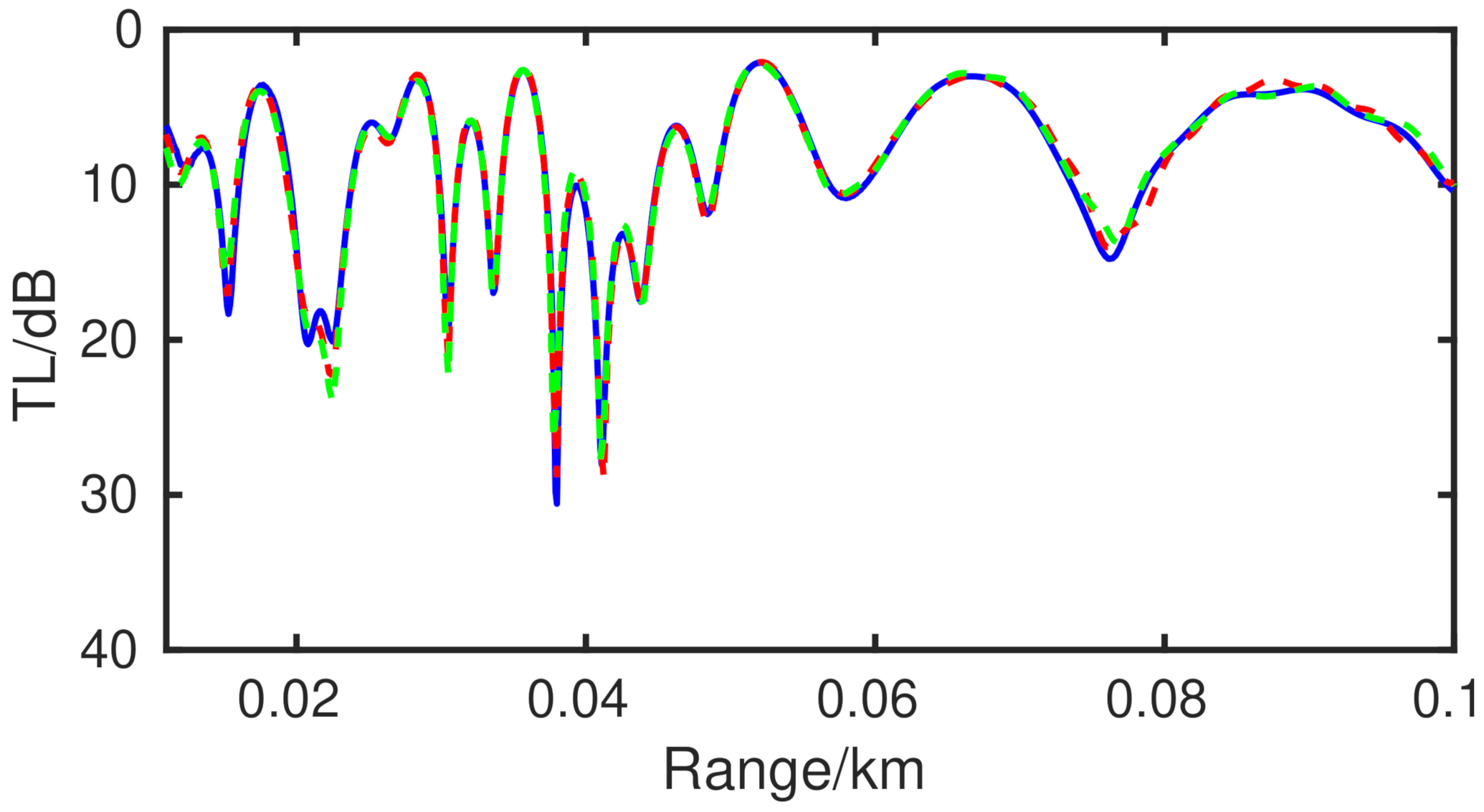
3.1. Range-Dependent Benchmark Problem

We consider the range-dependent benchmark problem first. In Figure 2, there is a wedge-shaped waveguide bounded above by a planar pressure-release sea surface and below by a planar rigid bottom. A line source is involved, parallel to the apex and located at $(r_{\mathrm{s}},{\theta }_{\mathrm{s}})$. The wedge angle is denoted by ${\theta }_0$. The analytical solution of sound field in the waveguide is [33]

$$\begin{array}{c}p(r,\theta )=\frac{\mathrm{i}\pi }{{\theta }_0}\sum _{n=1}^{\infty }sin\left({\gamma }_n{\theta }_{\mathrm{s}}\right)sin\left({\gamma }_n\theta \right){\mathrm{J}}_{{\gamma }_n}\left(k{r}_{<}\right){\mathrm{H}}_{{\gamma }_n}^{\left(1\right)}\left(k{r}_{>}\right),\\ {\gamma }_n=\left(n-\frac{1}{2}\right)\frac{\pi }{{\theta }_0},\\ r_{<}=min(r,r_{\mathrm{s}}),\\ r_{>}=max(r,r_{\mathrm{s}}),\end{array}$$

(23)

where $(r,\theta )$ is the polar coordinate representation of the observation point, $r_{\mathrm{s}}$ is the distance from the origin to the source, ${\theta }_{\mathrm{s}}$ is the angle between the x-axis and the line connecting the origin and the source, and ${\theta }_0$ is the inclination of the wedge-shaped waveguide.

Then, we will apply the presented finite element model to calculate the sound field in the wedge-shaped waveguide and compare its results with those by the above analytical solution. Figure 3 is the schematic diagram of specific environmental parameters of the wedge-shaped waveguide. The sound speed and density of sea water are $c=1500\mathrm{m}/\mathrm{s}$ and $\rho =1000\mathrm{kg}/{\mathrm{m}}^3$, respectively. The source frequency is $f=250\mathrm{Hz}$. The depth and range of source are $z_{\mathrm{s}}=20\mathrm{m}$ and $x_{\mathrm{s}}=50\mathrm{m}$, respectively. The inclination of the wedge is ${45}^{\circ }$.

Figure 4 is the sound field calculated by the analytical solution. An obvious interference pattern between the source and wedge vertex can be observed.

Then, we apply the presented finite element model to solve this problem. We discretize the wedge-shaped waveguide according to Figure 5 using four-node quadrilateral elements. If we use the traditional radiation boundary condition to simulate the boundless space, the elements from X to $X+{\delta }_x$ are needless and only the physical domain of sea water is discretized and calculated. The size of the elements is 0.5 m × 0.5 m.

Figure 6a is the sound field calculated by the finite element method with the traditional radiation boundary condition. It takes MATLAB almost 4 s to calculate on an i7-4790@3.60 GHz CPU. Figure 6b is obtained with the use of PML, where ${\sigma }_{xm}=50$, ${\delta }_x=6\mathrm{m}$, and the PML is divided into 15 layers vertically. It takes almost 10 s.

Compared with Figure 4, obvious error caused by interference can be seen in Figure 6a. This is because the traditional radiation boundary condition cannot totally absorb the outgoing wave—that is, the reflection coefficient at the boundary is not zero. However, the result in Figure 6b is consistent with that in Figure 4.

Figure 7 is the transmission loss in the wedge-shaped waveguide at 250 Hz at 10 m receiving depth. The blue solid line indicates the analytical solution, the red dashed line indicates finite element solution with traditional radiation boundary condition, and the green dashed line indicates finite element solution with PML. It can be seen that the green dashed line matches the blue solid line better, indicating that PML is more appropriate for simulating the boundless area than the traditional radiation boundary condition, and hence, yields higher precision.

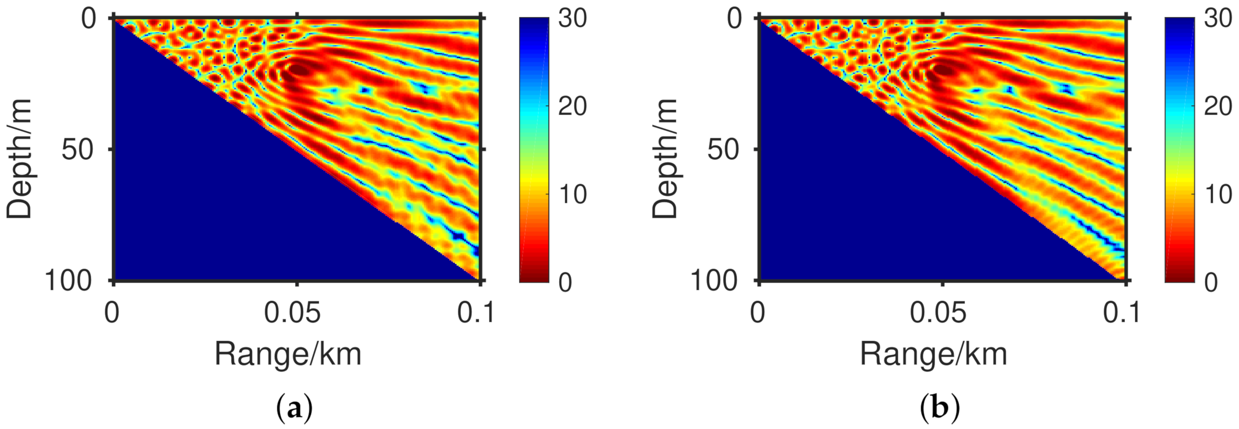
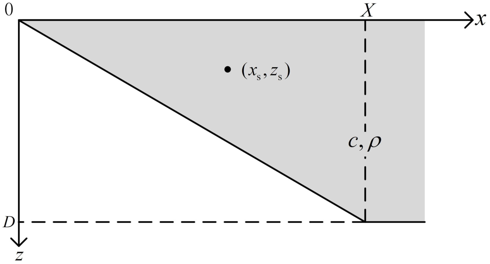
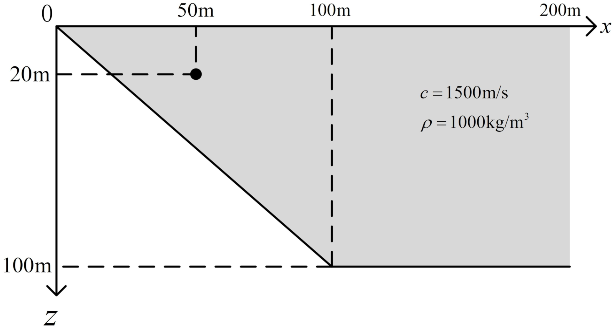
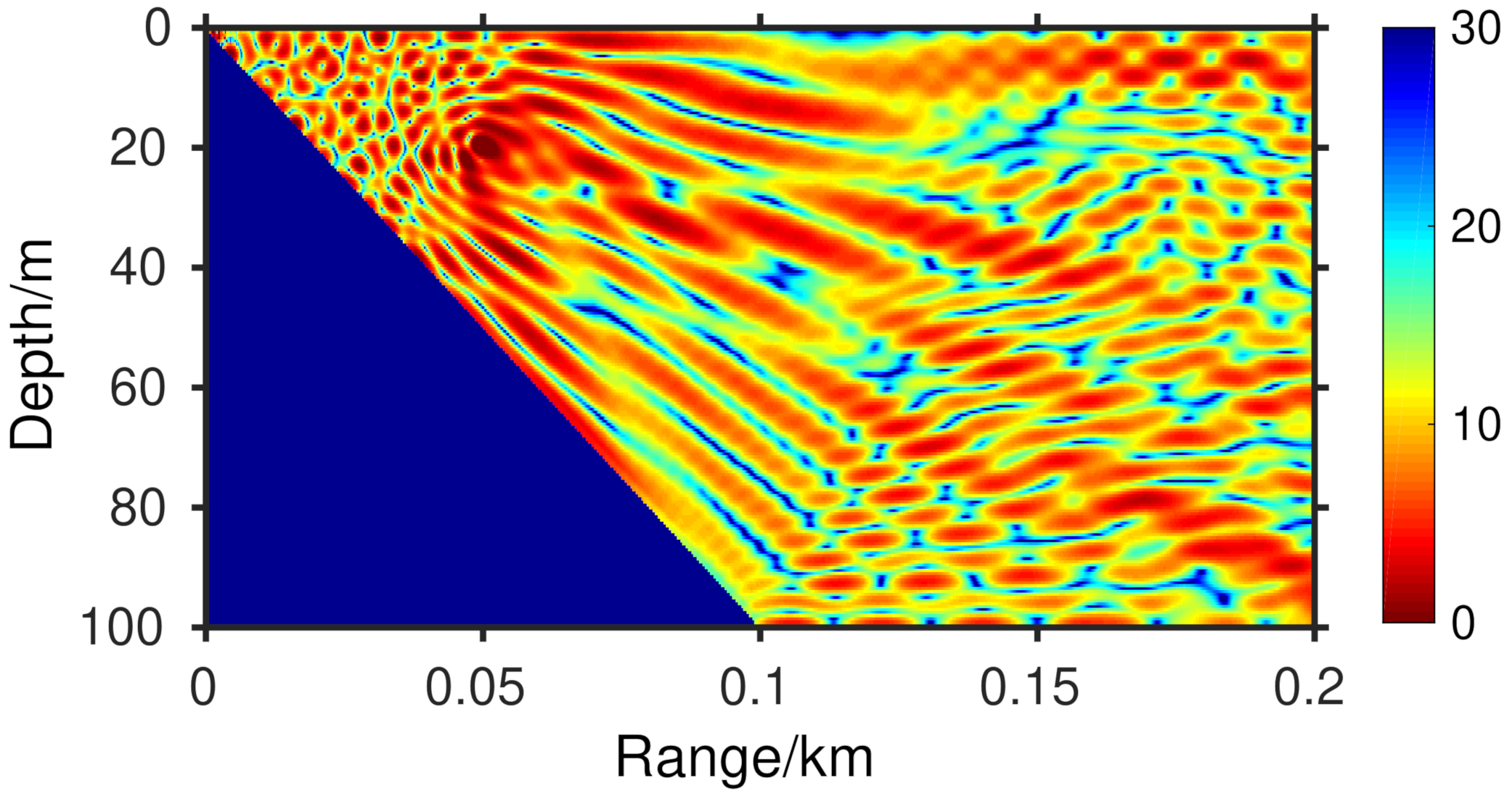
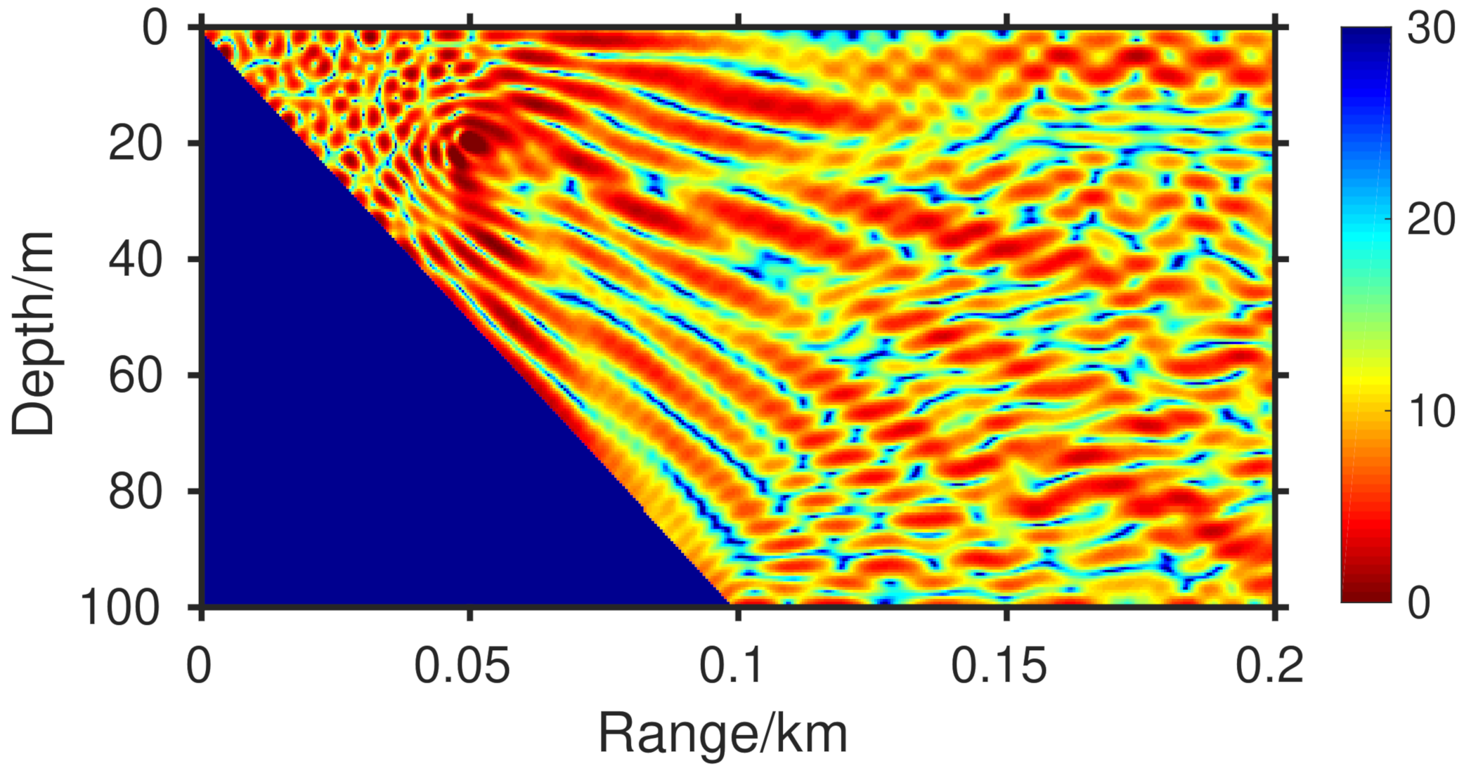
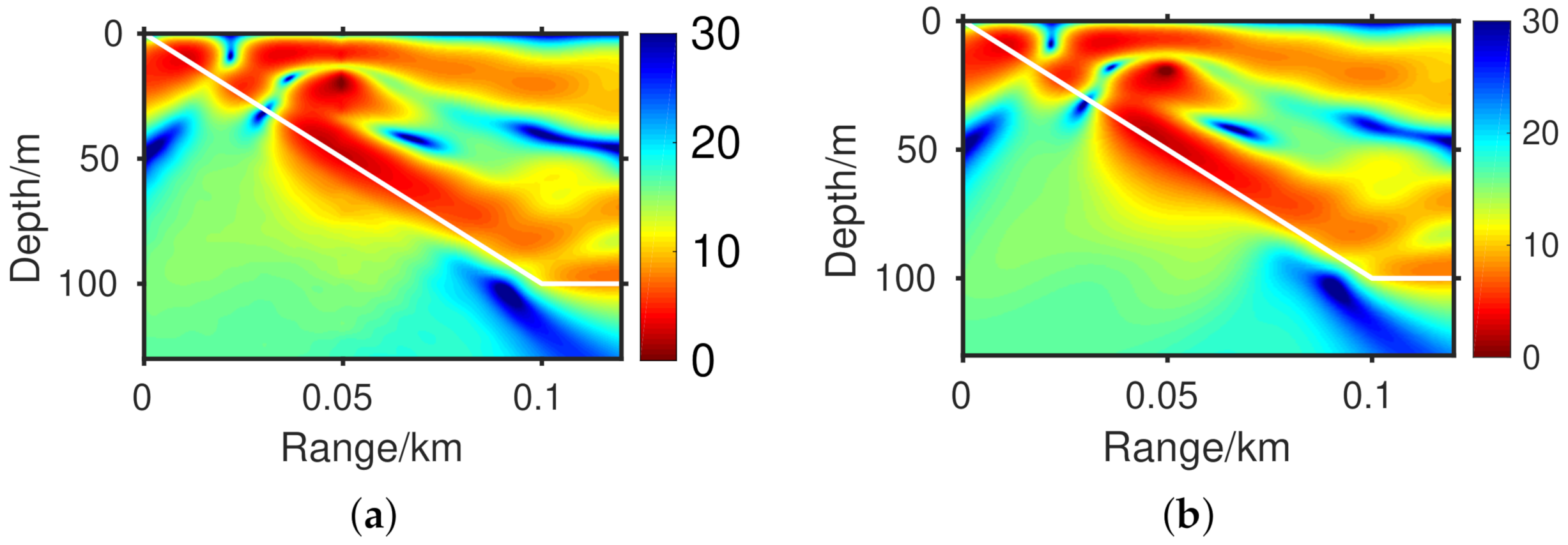
3.2. Slope Problem with Totally Reflected Bottom

Below, we consider the sound field of the wedge-shaped waveguide with a section of flat region, also called a slope problem. Figure 8 shows the schematic diagram of a slope-shaped waveguide. When $0<x<X$, there is a wedge-shaped waveguide. When $x>X$, there is a section of flat region. A line source is involved, which is parallel to the apex and located at $(x_{\mathrm{s}},z_{\mathrm{s}})$ in the wedge-shaped part. Since there is no analytical solution for this problem, the reference solution is provided by the coupled normal mode model DGMCM2D [34].

Then, we use the finite element method to calculate the sound field in specific slope-shaped waveguide environment and compare it with the reference solutions. Figure 9 is the schematic diagram of specific environmental parameters of a slope-shaped waveguide. The sound speed and density of sea water are $c=1500\mathrm{m}/\mathrm{s}$ and $\rho =1000\mathrm{kg}/{\mathrm{m}}^3$, respectively. The source frequency is $f=250\mathrm{Hz}$. The depth and range of source are $z_{\mathrm{s}}=20\mathrm{m}$ and $x_{\mathrm{s}}=50\mathrm{m}$, respectively.

Figure 10 is the reference solution of transmission loss calculated by DGMCM2D. An evident interference pattern is observed between the source and wedge vertex and also in the flat region, compared with Figure 4.

Then, we will use the finite element method to solve this problem. We discretize the slope-shaped waveguide according to Figure 11 using four-node quadrilateral elements. Only the physical domain of sea water is discretized and calculated. The area from $X_2$ to $X_2+{\delta }_x$ denotes the PML. The size of the elements is 0.5 m × 0.5 m.

Figure 12 is the transmission loss calculated by the finite element method with PML, where ${\sigma }_{xm}=50$, ${\delta }_x=12\mathrm{m}$ and the PML is divided into 15 layers vertically. It takes MATLAB almost 100 s to calculate on an i7-4790@3.60 GHz CPU.

Figure 13 is the transmission loss in the slope-shaped waveguide at 250 Hz at 10 m receiving depth. The blue solid line indicates the reference solution calculated by DGMCM2D and the red dashed line indicates the finite element solution with PML. It can be seen that the red dashed line matches very well with the blue solid line, indicating that the finite element model has high precision.

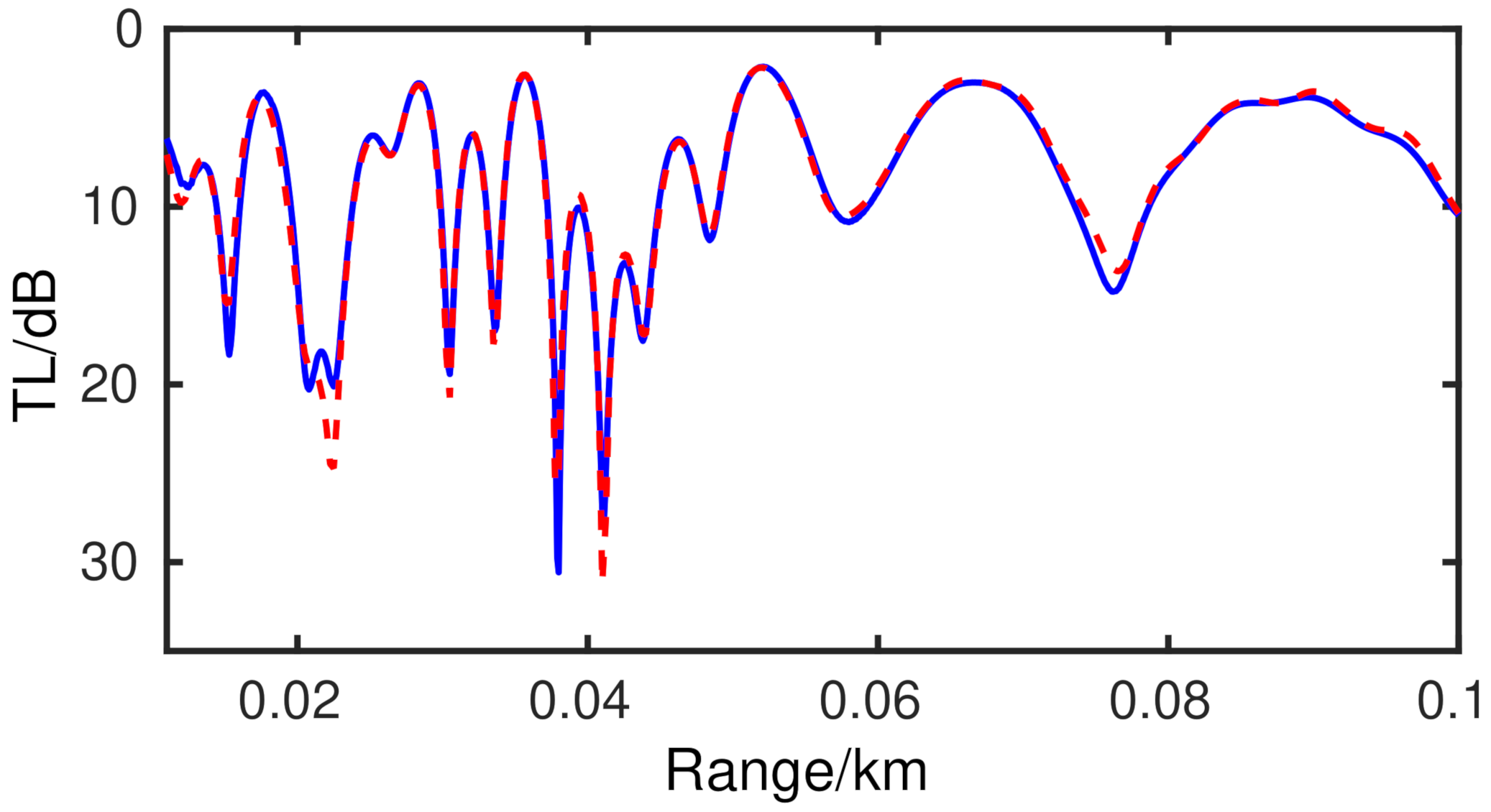
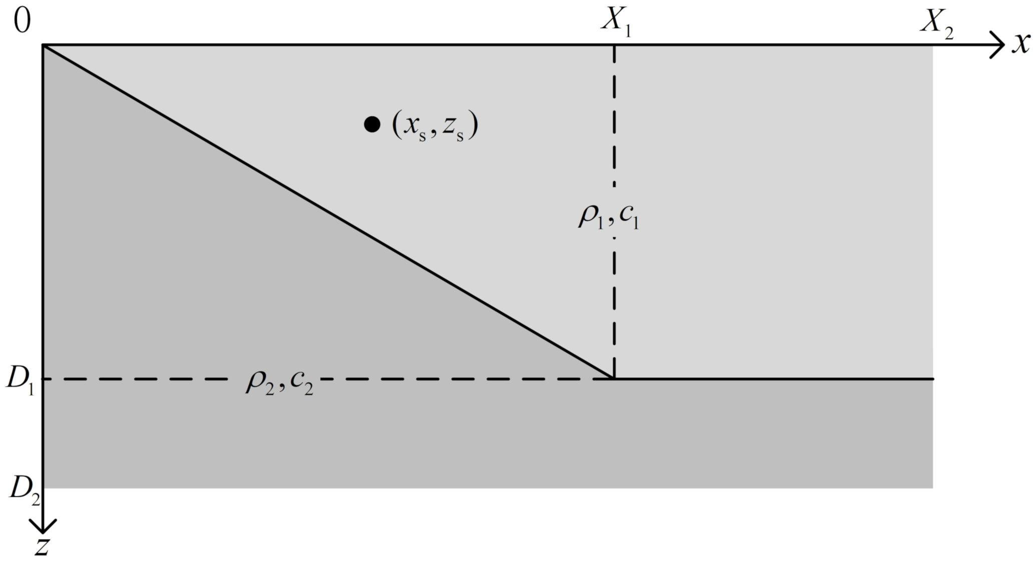
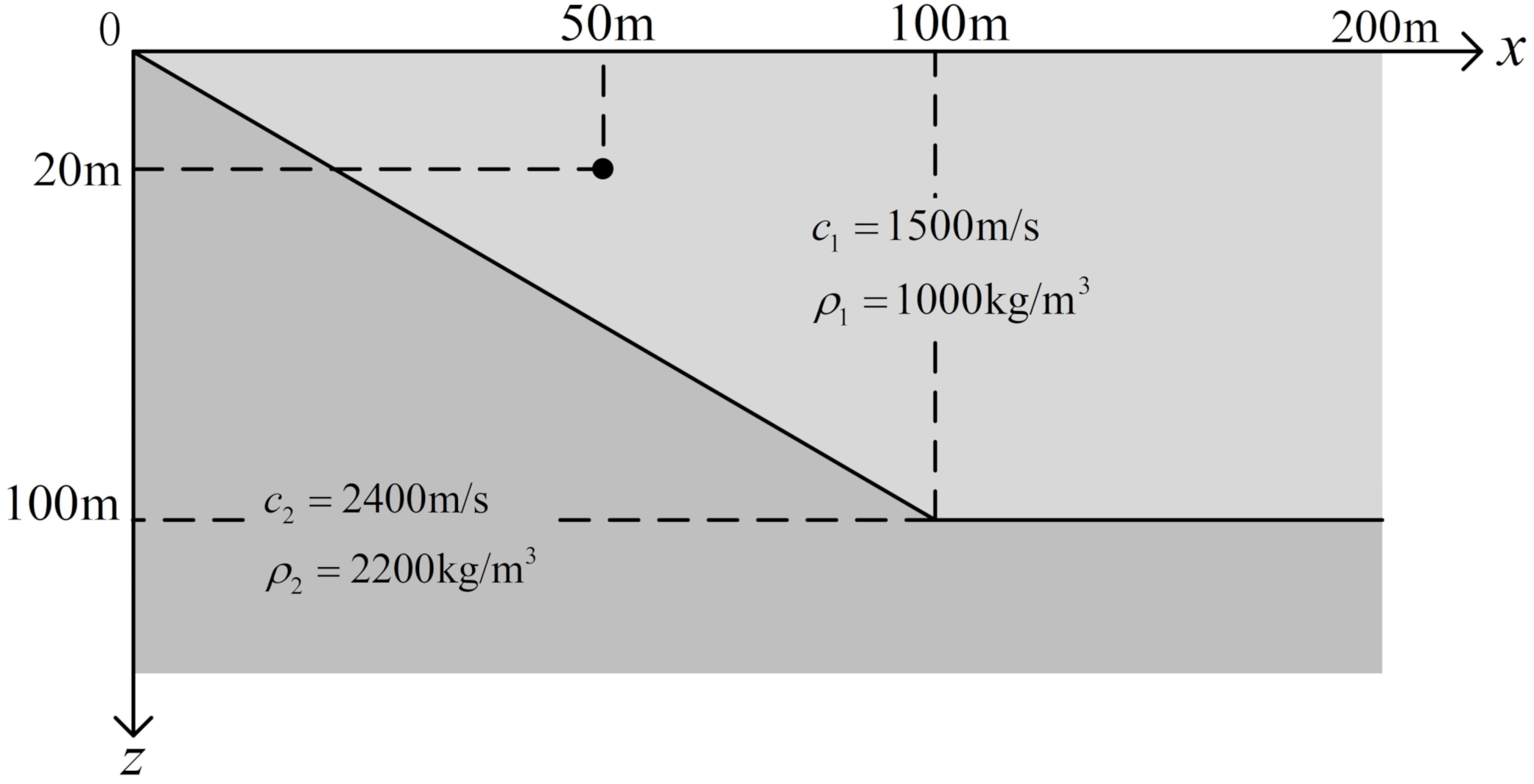
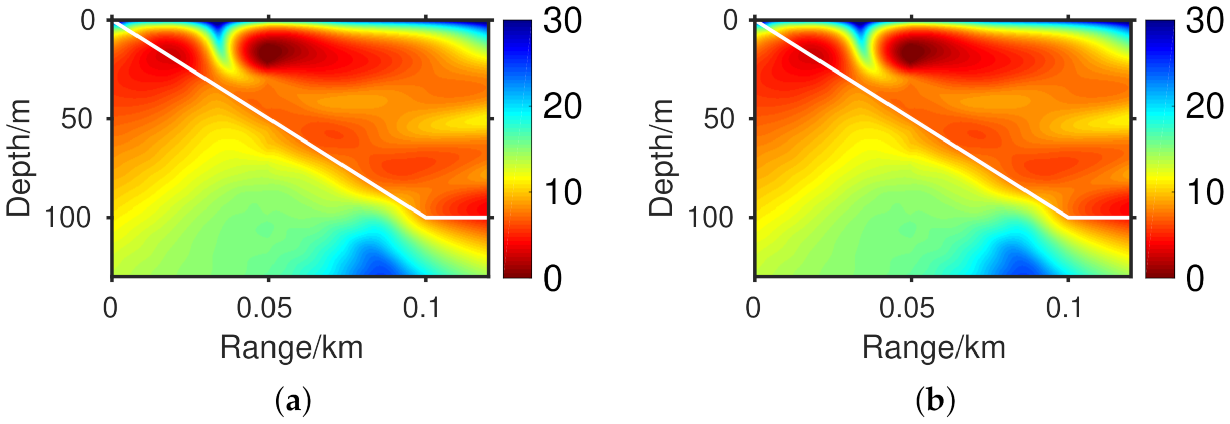
3.3. Slope Problem with Penetrable Bottom

As shown in the above sections, we have already seen the consistency between the finite element model and reference solution in a waveguide with a totally reflected bottom. Now, we will discuss the sound field in a waveguide with a penetrable bottom, as a slope bounded above by the sea surface and below by a penetrable bottom can be regarded as the simplest model of a shallow-sea waveguide near the coastline.

Figure 14 shows the schematic diagram of a slope with a penetrable bottom. $X_1<x<X_2$ denotes a section of flat region of sea water. A line source is involved, which is parallel to the apex and located at $(x_{\mathrm{s}},z_{\mathrm{s}})$.

For an environment with a penetrable bottom such as this problem, the physical domain is infinite not only in the horizontal direction but also in the vertical direction. As a result, we have to set a PML in the x-direction, a PML in the z-direction, and a PML in both the x- and z-directions, as Figure 15 shows. In ${\Omega }_{\mathrm{PML}x}=\left\{x\in (X_2,X_2+{\delta }_x),z\in (0,D_2)\right\}$, the coordinate transformation is only set on the x-axis, according to Equations (18)–(22), where $X=X_2$. Further, the coordinate transformation is only set on the z-axis in ${\Omega }_{\mathrm{PML}z}=\left\{x\in (0,X_2),z\in (D_2,D_2+{\delta }_z)\right\}$. We define the formation of $T\left(z\right)$ as

$$\tilde{z}=z-\mathrm{i}{\int }_{D_2}^{z-D_2}{\sigma }_z\left(\xi \right)\mathrm{d}\xi ,$$

(24)

$${\sigma }_z\left(\xi \right)={\sigma }_{zm}{\left(\frac{\xi }{{\delta }_z}\right)}^2,$$

(25)

where ${\sigma }_{zm}$ is a constant that decides the maximum loss in PML in the z-direction. From Equations (24) and (25), we can obtain

$$\frac{\mathrm{d}\tilde{z}}{\mathrm{d}z}=1-\mathrm{i}{\sigma }_z(z-D)=1-\mathrm{i}{\sigma }_{zm}{\left(\frac{z-\mathrm{D}}{{\delta }_z}\right)}^2,$$

(26)

$$\frac{\partial }{\partial z}=\frac{\partial }{\partial \tilde{z}}\frac{\mathrm{d}\tilde{z}}{\mathrm{d}z}\Rightarrow \frac{\partial }{\partial \tilde{z}}=\frac{\partial }{\partial z}{\left(\frac{\mathrm{d}\tilde{z}}{\mathrm{d}z}\right)}^{-1},$$

(27)

$$k_{mn}={\int \int }_{{\Omega }_{\mathrm{PML}z}}\frac{k^2{N}_n{N}_m}{\rho }\frac{\mathrm{d}\tilde{z}}{\mathrm{d}z}\mathrm{d}x\mathrm{d}z-{\int \int }_{{\Omega }_{\mathrm{PML}z}}\frac{1}{\rho }\left[\frac{\partial N_n}{\partial x}\frac{\partial N_m}{\partial x}\left(\frac{\mathrm{d}\tilde{z}}{\mathrm{d}z}\right)+\frac{\partial N_n}{\partial z}\frac{\partial N_m}{\partial z}{\left(\frac{\mathrm{d}\tilde{z}}{\mathrm{d}z}\right)}^{-1}\right]\mathrm{d}x\mathrm{d}z.$$

(28)

Here, $k_{mn}$ is the $(m,n)$th element of the local stiffness matrix of elements in ${\Omega }_{\mathrm{PML}z}$. As for ${\Omega }_{\mathrm{PML}xz}=\left\{x\in (X_2,X_2+{\delta }_x),z\in (D_2,D_2+{\delta }_z)\right\}$, coordinate transformation needs to be set on both the x- and z-axis—that is, both ${\sigma }_{xm}$ and ${\sigma }_{zm}$ are not zero in this area. We substitute Equations (19) and (25) into Equation (16) to obtain the elements of local stiffness matrices

$$\begin{array}{cc}\hfill k_{mn}=& {\int \int }_{{\Omega }_{\mathrm{PML}xz}}\frac{k^2{N}_n{N}_m}{\rho }\mathrm{d}\tilde{x}\mathrm{d}\tilde{z}-{\int \int }_{{\Omega }_{\mathrm{PML}x}}\frac{1}{\rho }\left(\frac{\partial N_n}{\partial \tilde{x}}\frac{\partial N_m}{\partial \tilde{x}}+\frac{\partial N_n}{\partial \tilde{z}}\frac{\partial N_m}{\partial \tilde{z}}\right)\mathrm{d}\tilde{x}\mathrm{d}\tilde{z}\hfill \\ \hfill =& {\int \int }_{{\Omega }_{\mathrm{PML}xz}}\frac{k^2{N}_n{N}_m}{\rho }\frac{\mathrm{d}\tilde{x}}{\mathrm{d}x}\frac{\mathrm{d}\tilde{z}}{\mathrm{d}z}\mathrm{d}x\mathrm{d}z\hfill \\ \hfill & -{\int \int }_{{\Omega }_{\mathrm{PML}xz}}\frac{1}{\rho }\left[\frac{\partial N_n}{\partial x}\frac{\partial N_m}{\partial x}{\left(\frac{\mathrm{d}\tilde{x}}{\mathrm{d}x}\right)}^{-1}\frac{\mathrm{d}\tilde{z}}{\mathrm{d}z}+\frac{\partial N_n}{\partial z}\frac{\partial N_m}{\partial z}\frac{\mathrm{d}\tilde{x}}{\mathrm{d}x}{\left(\frac{\mathrm{d}\tilde{z}}{\mathrm{d}z}\right)}^{-1}\right]\mathrm{d}x\mathrm{d}z.\hfill \end{array}$$

(29)

Then, we will use the finite element method to calculate the sound field in a specific slope-shaped waveguide environment with a penetrable bottom and compare it with the reference solution. Since there is no analytical solution for this problem, the reference solution is provided by DGMCM2D. It should be mentioned that for the wedge-shaped penetrable bottom problem, it is more appropriate to adopt the source images solution [35,36] as the reference solution. Figure 16 is the schematic diagram of specific environmental parameters. The sound speed and density of sea water are $c_1=1500\mathrm{m}/\mathrm{s}$ and ${\rho }_1=1000\mathrm{kg}/{\mathrm{m}}^3$; the sound speed and density of sediment are $c_2=2400\mathrm{m}/\mathrm{s}$ and ${\rho }_2=2200\mathrm{kg}/{\mathrm{m}}^3$; and the depth and range of source are $z_{\mathrm{s}}=20\mathrm{m}$ and $x_{\mathrm{s}}=50\mathrm{m}$, respectively. We will consider sound fields at the frequencies of $30\mathrm{Hz}$ and $50\mathrm{Hz}$.

For the case of the source frequency of 30 Hz, Figure 17a is the reference solution of transmission loss calculated by DGMCM2D and Figure 17b is calculated by the finite element model. It can be seen that the two sets of results are in excellent agreement.

For the case of the source frequency of 50 Hz, Figure 18a is the reference solution of transmission loss calculated by DGMCM2D and Figure 18b is calculated by finite element model. It is obvious that the two sets of results are also very consistent at 50 Hz.

3.4. Analysis of Universality

The accuracy of the presented finite element model has been demonstrated previously. Here, we discuss the universality of this finite element model compared with the normal mode model KRAKEN.

Consider the problem of sound propagation excited by a point source of strength $S_{\omega }$ in a Pekeris waveguide involving a homogeneous water column of depth $D_1$, sound speed $c_1$, and density ${\rho }_1$, overlying a homogeneous fluid half-space of sound speed $c_2$ and density ${\rho }_2$. A schematic of this problem is shown in Figure 19a. A Cartesian coordinate system is chosen, with the vertical z axis passing through the source and the x axis being parallel with the sea surface. The location of the source is denoted by $(0,z_{\mathrm{s}})$. For this problem, the two-dimensional Helmholtz equation for the displacement potential $\psi (x,z)$ takes the form

$$\left[\frac{{\partial }^2}{\partial x^2}+\frac{{\partial }^2}{\partial z^2}+k^2\left(z\right)\right]\psi (x,z)=S_{\omega }\delta \left(x\right)\delta (z-z_{\mathrm{s}}).$$

(30)

With the following Fourier transform pair,

$$\psi (x,z)={\int }_{-\infty }^{\infty }\Psi (k_x,z){\mathrm{e}}^{\mathrm{i}{k}_{x}x}\mathrm{d}{k}_x,$$

(31)

$$\Psi (k_x,z)=\frac{1}{2\pi }{\int }_{-\infty }^{\infty }\psi (x,z){\mathrm{e}}^{-\mathrm{i}{k}_{x}x}\mathrm{d}x,$$

(32)

the depth-dependent wave equation can be shown to be

$$\left[\frac{{\mathrm{d}}^2}{\mathrm{d}{z}^2}+(k^2-k_x^2)\right]\Psi (k_x,z)=S_{\omega }\frac{\delta (z-z_{\mathrm{s}})}{2\pi },$$

(33)

where $k_z^2=k^2-k_x^2$.

The depth-dependent Green’s function in the water $(0\le z\le D_1)$ is represented by [37]

$${\Psi }_1(k_x,z)=S_{\omega }\frac{{\mathrm{e}}^{\mathrm{i}{k}_{z1}|z-z_{\mathrm{s}}|}}{4\pi \mathrm{i}{k}_{z1}}+A_1^{+}{\mathrm{e}}^{\mathrm{i}{k}_{z1}z}+A_1^{-}{\mathrm{e}}^{-\mathrm{i}{k}_{z1}(z-D_1)},$$

(34)

where $k_{z,1}=\sqrt{k_1^2-k_x^2}$, with $k_1$ denoting the water wavenumber at frequency $\omega$. At the bottom $(z>D_1)$, the depth-dependent Green’s function is represented by

$${\Psi }_2(k_x,z)=A_2^{+}{\mathrm{e}}^{\mathrm{i}{k}_{z2}(z-D_1)},$$

(35)

where $k_{z,2}$ is the vertical wavenumber at the bottom, defined as follows, to satisfy the radiation condition for $z\to \infty$,

$$k_{z,2}=\left\{\begin{array}{cc}\sqrt{k_2^2-k_x^2},\hfill & |k_x|\le k_2,\hfill \\ \mathrm{i}\sqrt{k_x^2-k_2^2},\hfill & |k_x|>k_2,\hfill \end{array}\right.$$

(36)

with $k_2$ denoting the bottom wavenumber at frequency $\omega$. The amplitudes $A_1^{+}$, $A_1^{-}$, and $A_2^{+}$ are to be determined by the boundary conditions, as shown in Figure 19b.

By imposing the boundary conditions of vanishing pressure at the sea surface, and the continuity of the normal partial displacement and pressure at the bottom, we reach the following linear system of equations for the amplitudes of the solution to Equation (33).

$$\left[\begin{array}{ccc}1& {\mathrm{e}}^{\mathrm{i}{k}_{z1}{D}_1}& 0\\ k_{z1}{\mathrm{e}}^{\mathrm{i}{k}_{z1}{D}_1}& -k_{z1}& -k_{z2}\\ {\rho }_1{\mathrm{e}}^{\mathrm{i}{k}_{z1}{D}_1}& {\rho }_1& -{\rho }_2\end{array}\right]\left[\begin{array}{c}{A}_1^{+}\\ A_1^{-}\\ A_2^{+}\end{array}\right]=\frac{\mathrm{i}{S}_{\omega }}{4\pi k_{z1}}\left[\begin{array}{c}{\mathrm{e}}^{\mathrm{i}{k}_{z1}{z}_{\mathrm{s}}}\\ k_{z1}{\mathrm{e}}^{\mathrm{i}{k}_{z1}(D_1-z_{\mathrm{s}})}\\ {\rho }_1{\mathrm{e}}^{\mathrm{i}{k}_{z1}(D_1-z_{\mathrm{s}})}\end{array}\right].$$

(37)

Once the amplitudes $A_1^{+}$, $A_1^{-}$, and $A_2^{+}$ are obtained by solving the above linear system of equations, the depth-dependent Green’s function can then be evaluated by Equations (34) and (35). Then, the displacement potential $\psi (x,z)$ can be computed by evaluating the inverse Fourier transform given in Equation (31).

The transmission loss for the line source problem is defined by

$$\mathrm{TL}(x,z)=-20{log}_{10}\left|\frac{p(x,z)}{p_0(r=1)}\right|,$$

(38)

where

$$p(x,z)=\left\{\begin{array}{cc}{\rho }_1{\omega }^2{\psi }_1(x,z),\hfill & 0\le z\le D_1,\hfill \\ {\rho }_2{\omega }^2{\psi }_2(x,z),\hfill & z>D_1,\hfill \end{array}\right.$$

(39)

and the reference pressure takes the form (assuming the line source is located in water)

$$p_0\left(r\right)=(-{\rho }_1{\omega }^2{S}_{\omega })\frac{\mathrm{i}}{4}{\mathrm{H}}_0^{\left(1\right)}\left(k_{0}r\right).$$

(40)

The solution calculated by the wavenumber integration method can serve as the benchmark solution.

We now consider a specific environment, as schematically shown in Figure 20. The source depth is 20 m. The sound speed and density in water are 1500 m/s and $1000\mathrm{kg}/{\mathrm{m}}^3$, respectively; the sound speed and density at the bottom are 1650 m/s and $1500\mathrm{kg}/{\mathrm{m}}^3$, respectively.

We firstly calculate the transmission loss with frequency from 105 Hz to 125 Hz. Figure 21 shows the results of transmission loss versus range and frequency at 40 m receiver depth using different methods. The horizontal axis denotes range and the longitudinal axis denotes frequency. Figure 21a is the transmission loss calculated by the popular normal mode model, KRAKEN. Figure 21b is calculated by the wavenumber integration method given above, which is regarded as the standard solution. Figure 21c is calculated by the finite element model. It can be seen from Figure 21 that the finite element solution is consistent with the standard solution. However, the result calculated by KRAKEN shows obvious errors at certain frequencies. It is evident that the result by KRAKEN is irregular around 112 Hz, whereas the results by the finite element model and by the wavenumber integration method are in excellent agreement. Below, we will consider two specific frequencies, 112 Hz and 118 Hz.

The depth-dependent Green’s function at depth 40 m calculated by Equation (34) at frequencies 112 Hz and 118 Hz are shown in Figure 22a,b, respectively, where the bottom wavenumbers are indicated by the red dashed lines. Figure 22c,d show results of transmission loss versus range at a depth of 40 m computed by the wavenumber integration method (blue solid lines), KRAKEN (green dashed lines), and the finite element model (red dashed lines) at the two specific frequencies—112 Hz and 118 Hz. At frequency 112 Hz, the bottom wavenumber is approximately $0.426495{\mathrm{m}}^{-1}$, while the horizontal wavenumbers of the first five modes by KRAKEN are 0.464455, 0.449802, 0.381011 + 0.916079E-2i, 0.309800 + 0.178554E-1i, 0.188504 + 0.392254E-1i. At frequency 118 Hz the bottom wavenumber is approximately $0.449343{\mathrm{m}}^{-1}$, while the horizontal wavenumbers of the first five modes by KRAKEN are 0.489759, 0.475685, 0.451877, 0.411541 + 0.790571E-2i, and 0.346650 + 0.154633E-1i. From Figure 22a, we can see that at frequency 112 Hz, the horizontal wavenumber of mode 3 is so close to the bottom wavenumber, which is the branch point for this problem, that KRAKEN fails to find this mode. As a result, as shown in Figure 21 and Figure 22c, the field results of KRAKEN are inaccurate. However, at frequency 118 Hz, Figure 22b shows that the horizontal wavenumber of mode 3 is sufficiently far away from the bottom wavenumber such that KRAKEN succeeds in finding this mode. As a result, as shown in Figure 21 and Figure 22d, the field results by KRAKEN are in excellent agreement with the standard solution calculated by the wavenumber integration method. In addition, it is evident from Figure 21 and Figure 22 that the results by the finite element model and the wavenumber integration method are in excellent agreement throughout the whole frequency band of interest.

The above numerical results indicate that the finite element model can provide accurate field results for general Pekeris problems and is well-suited for the problems of sound propagation. However, in the special case where a mode lies very close to the branch cut, KRAKEN might fail to provide accurate field results due to the neglect of the branch line integral. For a single-frequency calculation, the probability of the occurrence of a mode lying near the branch cut is not great. For broadband calculations, however, the probability is high. Another scenario with a high probability encountering this phenomenon for single-frequency problems is when the bathymetry varies with range. However, the finite element method calculates the sound field by forming the stiffness matrix and the load vector and is stable wherever the branch cut is. As a result, the finite element model has more universality than KRAKEN.

4. Conclusions

In this paper, we introduce a finite element model in Cartesian coordinates for underwater sound field calculation in a two-dimensional environment.

At the beginning, the details of implementation were given. We firstly derived the weak form of the Helmholtz equation using the Galerkin method, then discretized the physical domain using four-node quadrilateral elements, and introduced the calculation of local stiffness matrices and assembly of global stiffness matrix.

Then, different methods to deal with boundary conditions, especially simulating the boundless area, were discussed and compared. The Dirichlet boundary and Neumann boundary were easy to deal with. As for the boundless area—that is, regarding how to set an artificial boundary condition to simulate media in an infinite area, we compared the traditional radiation boundary condition and perfectly matched layer approach and found that the traditional radiation boundary may cause noticeable errors because of the nonzero reflection coefficient at the artificial boundary.

After that, range-dependent problems were calculated using the finite element model, such as the wedge-shaped benchmark problem and the slope problem, with either a totally reflected bottom or a penetrable bottom. All of the problems were solved with satisfying results.

In the end, we took the Pekeris waveguide problem as an example to illustrate the universality of the presented finite element model. We used the wavenumber integration method to provide the benchmark solution and compared the results calculated by KRAKEN and the finite element model. The results show that KRAKEN may be inaccurate at the frequencies where a mode lies too close to the branch cut, whereas the results of our finite element model are in excellent agreement with the benchmark solution.

In summary, our finite element model has the following advantages:

• High accuracy. Our finite element model achieves high accuracy in both range-dependent problems and inhomogeneous media problems.
• Great universality. Compared with the popular KRAKEN model, our finite element model has better universality and is well-suited for more complex problems.
• Focused on range-dependent underwater sound propagation problems.
• Flexible. Since our model is entirely developed by ourselves instead of relying on commercial software, it is easier to modify and optimize.

However, there are still shortcomings of the model, as listed below; we will improve this model in the future. The work in this paper forms a solid foundation for future research.

• The integral method. While calculating the elements of stiffness matrices, we used the trapezoid method to evaluate the integral, which is not efficient enough. We will try other methods, such as the Gauss integral method, to improve the accuracy and efficiency.
• The selection of meshes. Only four-node quadrilateral elements are used in this model. As a result, when calculating the sound field in a complex environment especially with complex shape of boundaries, the meshes cannot match the boundaries very well. We plan to optimize the selection of meshes, combining triangular elements and quadrilateral elements to discretize the physical domain.

In conclusion, in this paper, a finite element model has been presented to calculate the underwater sound field in complex environments with high precision and great universality.

References

1. Clough, R.W. The finite element method in plane stress analysis. In Proceedings of the 2nd ASCE Conference on Electronic Computation, Pittsburgh, PA, USA, 8–9 September 1960. [Google Scholar]
2. Gladwell, G. A variational formulation of damped acousto structural vibration problems. J. Sound Vib. 1966, 4, 172–186. [Google Scholar] [CrossRef]
3. Craggs, A. The use of simple three-dimensional acoustic finite elements for determining the natural modes and frequencies of complex shaped enclosures. J. Sound Vib. 1972, 23, 331–339. [Google Scholar] [CrossRef]
4. Nefske, D.; Wolf, J., Jr.; Howell, L. Structural-acoustic finite element analysis of the automobile passenger compartment: A review of current practice. J. Sound Vib. 1982, 80, 247–266. [Google Scholar] [CrossRef]
5. Hunt, J.T.; Knittel, M.R.; Barach, D. Finite element approach to acoustic radiation from elastic structures. J. Acoust. Soc. Am. 1974, 55, 269–280. [Google Scholar] [CrossRef]
6. Hunt, J.T.; Knittel, M.R.; Nichols, C.S.; Barach, D. Finite- element approach to acoustic scattering from elastic structures. J. Acoust. Soc. Am. 1975, 57, 287–299. [Google Scholar] [CrossRef]
7. Bettess, P. Infinite elements. Int. J. Numer. Methods Eng. 1977, 11, 53–64. [Google Scholar] [CrossRef]
8. Astley, R.; Coyette, J.P. The performance of spheroidal infinite elements. Int. J. Numer. Methods Eng. 2001, 52, 1379–1396. [Google Scholar] [CrossRef]
9. Berenger, J.P. A perfectly matched layer for the absorption of electromagnetic waves. J. Comput. Phys. 1994, 114, 185–200. [Google Scholar] [CrossRef]
10. Berenger, J.P. Perfectly matched layer for the FDTD solution of wave-structure interaction problems. IEEE Trans. Antennas Propag. 1996, 44, 110–117. [Google Scholar] [CrossRef]
11. Givoli, D. High-order local non-reflecting boundary conditions: A review. Wave Motion 2004, 39, 319–326. [Google Scholar] [CrossRef]
12. Givoli, D. Recent advances in the DtN FE method. Arch. Comput. Methods Eng. 1999, 6, 71–116. [Google Scholar] [CrossRef]
13. Thompson, L.L.; Pinsky, P.M. Encyclopedia of Computational Mechanics: Acoustics; Wiley: Hoboken, NJ, USA, 2004. [Google Scholar]
14. Harari, I.; Hughes, T.J. A cost comparison of boundary element and finite element methods for problems of time-harmonic acoustics. Comput. Methods Appl. Mech. Eng. 1992, 97, 77–102. [Google Scholar] [CrossRef]
15. Harari, I.; Hughes, T.J. Analysis of continuous formulations underlying the computation of time-harmonic acoustics in exterior domains. Comput. Methods Appl. Mech. Eng. 1992, 97, 103–124. [Google Scholar] [CrossRef]
16. Chew, W.C.; Song, J.; Cui, T.; Velamparambil, S.; Hastriter, M.; Hu, B. Review of large scale computing in electromagnetics with fast integral equation solvers. CMES-Comput. Model. Eng. Sci. 2004, 5, 361–372. [Google Scholar]
17. Fischer, M.; Gaul, L. Fast BEM–FEM mortar coupling for acoustic–structure interaction. Int. J. Numer. Methods Eng. 2005, 62, 1677–1690. [Google Scholar] [CrossRef]
18. Van Hal, B.; Desmet, W.; Vandepitte, D.; Sas, P. A coupled finite element–wave based approach for the steady-state dynamic analysis of acoustic systems. J. Comput. Acoust. 2003, 11, 285–303. [Google Scholar] [CrossRef]
19. Murphy, J.E.; Chin-Bing, S.A. A finite element model for ocean acoustic propagation. Math. Comput. Model. 1988, 11, 70–74. [Google Scholar] [CrossRef]
20. Murphy, J.E.; Chin-Bing, S.A. A finite-element model for ocean acoustic propagation and scattering. J. Acoust. Soc. Am. 1989, 86, 1478–1483. [Google Scholar] [CrossRef]
21. Murphy, J.E.; Chin-Bing, S.A. A seismo-acoustic finite element model for underwater acoustic propagation. In Shear Waves in Marine Sediments; Springer: Berlin/Heidelberg, Germany, 1991; pp. 463–470. [Google Scholar]
22. Kampanis, N.A.; Dougalis, V.A. A finite element code for the numerical solution of the Helmholtz equation in axially symmetric waveguides with interfaces. J. Comput. Acoust. 1999, 7, 83–110. [Google Scholar] [CrossRef]
23. Jun, L. Numerical Solution of Sound Field in Shallow Water by Finite Element Method. Ph.D. Thesis, Peking University, Beijing, China, 2005. [Google Scholar]
24. Athanassoulis, G.; Belibassakis, K.; Mitsoudis, D.; Kampanis, N.; Dougalis, V. Coupled mode and finite element approximations of underwater sound propagation problems in general stratified environments. J. Comput. Acoust. 2008, 16, 83–116. [Google Scholar] [CrossRef]
25. Junyu, F. Research on Finite Element Method in Ocean Acoustic Propagation Problems. Master’s Thesis, Harbin Engineering University, Harbin, China, 2016. [Google Scholar]
26. Jun, Z. Research on Ocean Sound Propagation Characteristics Based on Finite Element Method. Master’s Thesis, Zhejiang Ocean University, Zhoushan, China, 2019. [Google Scholar]
27. Goldsberry, B.M.; Isakson, M. Comparison of two-dimensional axial-symmetric and longitudinally invariant methods for three-dimensional shallow water acoustic propagation using finite element methods. In Proceedings of the Meetings on Acoustics ICA2013, Montreal, QC, Canada, 2–7 June 2013; Acoustical Society of America: New York, NY, USA, 2013; Volume 19, p. 070080. [Google Scholar]
28. Chai, Y.; Gong, Z.; Li, W.; Li, T.; Zhang, Q.; Zou, Z.; Sun, Y. Application of smoothed finite element method to two-dimensional exterior problems of acoustic radiation. Int. J. Comput. Methods 2018, 15, 1850029. [Google Scholar] [CrossRef]
29. Chai, Y.; Li, W.; Gong, Z.; Li, T. Hybrid smoothed finite element method for two-dimensional underwater acoustic scattering problems. Ocean Eng. 2016, 116, 129–141. [Google Scholar] [CrossRef]
30. Chai, Y.; You, X.; Li, W.; Huang, Y.; Yue, Z.; Wang, M. Application of the edge-based gradient smoothing technique to acoustic radiation and acoustic scattering from rigid and elastic structures in two dimensions. Comput. Struct. 2018, 203, 43–58. [Google Scholar] [CrossRef]
31. Jensen, F.B.; Kuperman, W.A.; Porter, M.B.; Schmidt, H. Computational Ocean Acoustics; Springer: New York, NY, USA, 2011. [Google Scholar]
32. Liu, L.; Qin, Y.; Xu, Y.; Zhao, Y. The uniqueness and existence of solutions for the 3-D Helmholtz equation in a stratified medium with unbounded perturbation. Math. Methods Appl. Sci. 2013, 36, 2033–2047. [Google Scholar] [CrossRef]
33. Wen-Yu, L.; Chun-Mei, Y.; Ji-Xing, Q.; Zhang, R.H. Benchmark solutions for sound propagation in an ideal wedge. Chin. Phys. B 2013, 22, 054301. [Google Scholar]
34. Luo, W.; Yang, C.; Qin, J.; Zhang, R. A numerically stable coupled-mode formulation for acoustic propagation in rage-dependent waveguides. Sci. China Phys. Mech. Astron. 2012, 55, 572–588. [Google Scholar] [CrossRef]
35. Deane, G.; Buckingham, M. An analysis of the three-dimensional sound field in a penetrable wedge with a stratified fluid or elastic basement. J. Acoust. Soc. Am. 1993, 93, 1319–1328. [Google Scholar] [CrossRef]
36. Tang, J.; Petrov, P.; Piao, S.; Kozitskiy, S. On the Method of Source Images for the Wedge Problem Solution in Ocean Acoustics: Some Corrections and Appendices. Acoust. Phys. 2018, 64, 228–240. [Google Scholar] [CrossRef]
37. Luo, W.Y.; Yu, X.L.; Yang, X.F.; Zhang, R.H. Analytical solution based on the wavenumber integration method for the acoustic field in a Pekeris waveguide. Chin. Phys. B 2016, 25, 044302. [Google Scholar] [CrossRef]
Figure 1. Schematic diagram of local indices, midpoint coordinates, length, and width of the four-node quadrilateral element.
Jmse 09 00956 g001
Figure 2. Schematic diagram of a wedge-shaped waveguide bounded above by a planar pressure-release sea surface and below by a planar rigid bottom. A line source is involved, which is parallel to the apex and located at ( r s , θ s ) . The inclination of the waveguide is denoted by θ 0 .
Jmse 09 00956 g002
Figure 3. Schematic diagram of specific environmental parameters of a wedge-shaped waveguide.
Jmse 09 00956 g003
Figure 4. Analytical solution of transmission loss in a wedge-shaped waveguide at 250 Hz calculated by Equation (23).
Jmse 09 00956 g004
Figure 5. Schematic diagram of discretization of physical domain and PML in a wedge-shaped waveguide using four-node quadrilateral elements.
Jmse 09 00956 g005
Figure 6. Transmission loss in a wedge-shaped waveguide at 250 Hz calculated by the finite element method (a) with traditional radiation condition and (b) with perfectly matched layer.
Jmse 09 00956 g006
Figure 7. Transmission loss in a wedge-shaped waveguide at 250 Hz at 10 m receiving depth. The source depth is 20 m and the horizontal distance is 50 m. The blue solid line indicates analytical solution, the red dashed line indicates finite element solution with traditional radiation boundary condition, and the green dashed line indicates finite element solution with PML.
Jmse 09 00956 g007
Figure 8. Schematic diagram of a slope-shaped waveguide bounded above by a planar pressure-release sea surface and below by a rigid bottom. A line source is involved, which is parallel to the apex and located at ( x s , z s ) .
Jmse 09 00956 g008
Figure 9. Schematic diagram of specific environmental parameters of a slope-shaped waveguide.
Jmse 09 00956 g009
Figure 10. Reference solution of transmission loss in a slope-shaped waveguide at 250 Hz calculated by DGMCM2D.
Jmse 09 00956 g010
Figure 11. Schematic diagram of discretization of physical domain in a slope-shaped waveguide using four-node quadrilateral elements.
Jmse 09 00956 g011
Figure 12. Transmission loss in a slope-shaped waveguide at 250 Hz calculated by finite element method with PML.
Jmse 09 00956 g012
Figure 13. Transmission loss in a slope-shaped waveguide at 250 Hz at 10 m receiving depth. The source depth is 20 m and the horizontal distance is 50 m. The blue solid line indicates reference solution calculated by DGMCM2D and the red dashed line indicates finite element solution with PML.
Jmse 09 00956 g013
Figure 14. Schematic diagram of a slope with penetrable bottom and a planar pressure-release sea surface. A line source is involved, which is parallel to the apex and located at ( x s , z s ) .
Jmse 09 00956 g014
Figure 15. Schematic diagram of a slope with penetrable bottom and perfectly matched layers.
Jmse 09 00956 g015
Figure 16. Schematic diagram of specific environmental parameters of a slope-shaped waveguide with a penetrable sea bottom.
Jmse 09 00956 g016
Figure 17. Transmission loss at 30 Hz in a slope-shaped waveguide with a penetrable bottom. (a) Calculated by DGMCM2D. (b) Calculated by the finite element model.
Jmse 09 00956 g017
Figure 18. Transmission loss at 50 Hz in a slope-shaped waveguide with a penetrable bottom. (a) Calculated by DGMCM2D. (b) Calculated by the finite element model.
Jmse 09 00956 g018
Figure 19. Pekeris waveguide with unlimited depth. (a) Schematic diagram of the environment. (b) Schematic diagram of upgoing and downgoing waves in two-layer medium.
Jmse 09 00956 g019
Figure 20. Schematic diagram of specific environmental parameters of two-layer medium with unlimited depth.
Jmse 09 00956 g020
Figure 21. Transmission loss at depth of 40 m from 105 Hz to 125 Hz using different methods. (a) Solution calculated by normal mode model KRAKEN. (b) Benchmark solution calculated by wavenumber integration method. (c) Finite element solution.
Jmse 09 00956 g021
Figure 22. (a) Magnitude of the depth-dependent Green’s function at a depth of 40 m at 112 Hz; (b) transmission loss at a depth of 40 m at 112 Hz; (c) magnitude of the depth-dependent Green’s function at a depth of 40 m at 118 Hz; (d) transmission loss at a depth of 40 m at 118 Hz. In panels (a,c), the red dashed lines indicate bottom wavenumbers. In panels (b,d), the blue solid lines indicate benchmark solution calculated by wavenumber integration method, the red dashed lines indicate finite element solution, and the green dashed lines indicate transmission loss calculated by KRAKEN model.
Jmse 09 00956 g022
Publisher’s Note: MDPI stays neutral with regard to jurisdictional claims in published maps and institutional affiliations.