An Improved Failure Risk Assessment Method for Bilge System of the Large Luxury Cruise Ship under Fire Accident Conditions

Abstract

This paper develops an improved failure risk assessment method and discusses the risk control measures for a large luxury cruise ship’s bilge system under fire accident conditions. The proposed method incorporates an expert weight calculation model and a risk coefficient calculation model. The expert weight calculation model considers the differences in experts’ expertise levels (i.e., qualification level, decision-making capacity, and decision-making preference). Further, the method integrates the evaluations resulting from fuzzy analytic hierarchy process (FAHP) and extended fuzzy technique for order preference by similarity to ideal solution (FTOPSIS) of different experts. The risk coefficient (RC) calculation model utilizes a three-dimensional continuous matrix, serving to determine the risk factors’ ratings. The influences of the expert weight and RC calculation models on the proposed method’s performance are studied through a sensitivity analysis. The work demonstrates that the proposed method minimizes the issues encountered when using conventional methods for determining risk ratings. Finally, the results of an empirical study comprising ten experts evaluating the VISTA cruise ship’s bilge system prove the applicability of the proposed method and offer practical design guidelines to meet the regulations for Safe Return to Port (SRtP).

1. Introduction

1.1. Background

The international cruise industry is at a rapid developing time, marked by a strong interest in tourism and significant investments by cruise companies in numerous sophisticated ships [1]. Such ships are characterized by a large number of passengers, large dimensions, long sailing time, and high commercial value [2]. However, compared to conventional ships (i.e., cargo and container ships) and inland vehicles, cruise accidents are more likely to cause significant accidents. For this reason, the International Maritime Organization (IMO), Cruise Lines International Association (CLIA), Lloyd’s Register of Shipping (LR), and other organizations have issued strict specifications related to passenger ship design and construction.

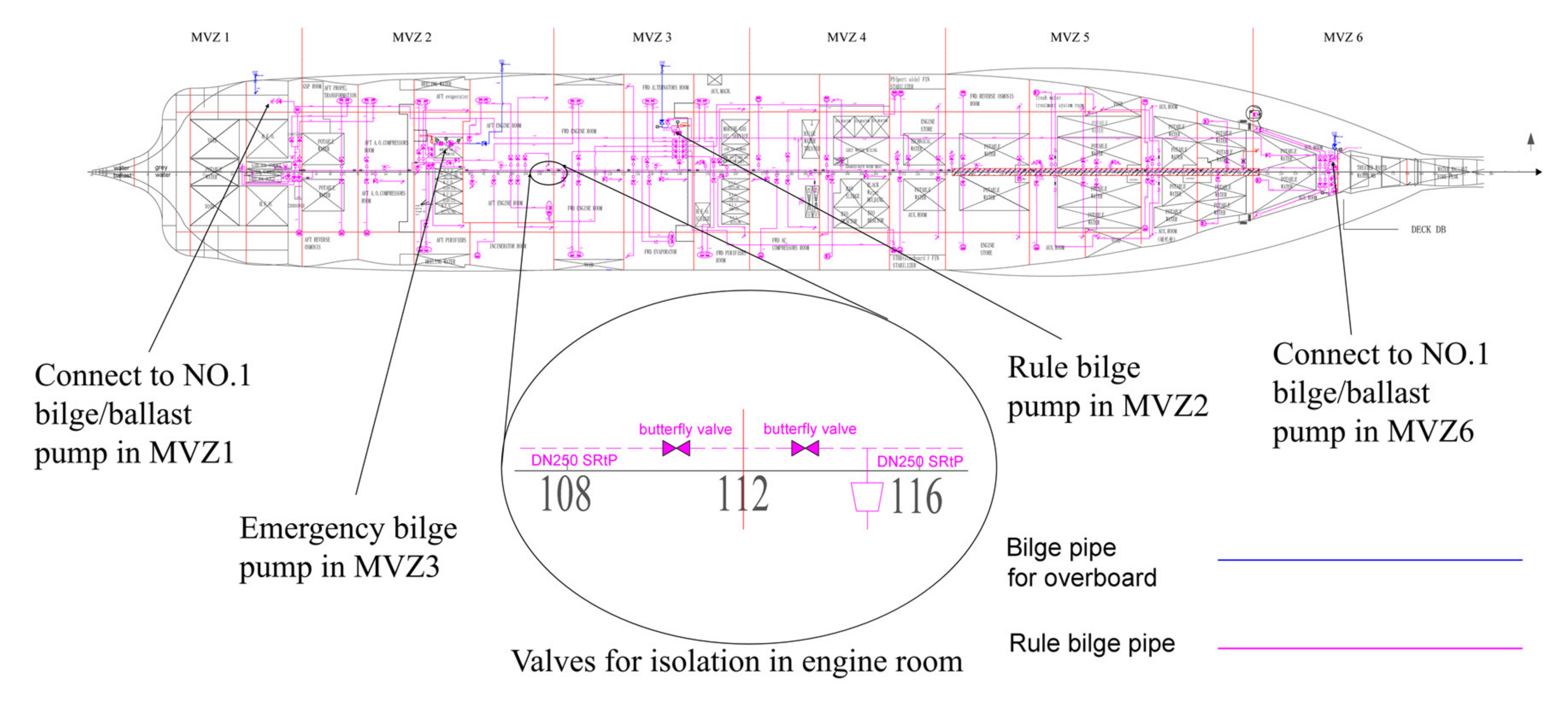
Cruise ship bilge systems are one of the most important auxiliary systems for cruise ship safety and typically consist of an oily bilge system and a rule bilge system. The oily bilge system is responsible for collecting and treating oily bilge water, whereas the rule bilge water system serves to timely discharge floodwater and firewater in case of emergency. Similar to a cargo ship, the large luxury cruise ship’s bilge system consists of elements such as a bilge pump, main bilge pipe, and valves. Several bilge-system components are adjacent to high-risk areas or high-temperature heat sources (e.g., engine room, generator, and fuel tank), creating a potential hazard [3]. Since these components could be seriously affected by a fire accident, they are viewed as parts of the high-risk factors in a bilge system. However, qualitative analyses may not accurately identify predominant risk factors. Therefore, the main aspect of failure risk assessment is to determine the predominant risk factors. With regards to the ship piping system [4], the bilge-system risk factors can be categorized into four categories (i.e., power machinery, facility, pipeline, measuring instrument), as further discussed in Section 4, that serve as attributes in decision-making.

The International Convention for Safety of Life at Sea (SOLAS) has put forward requirements for the reliability of the bilge system in the event of a ship fire [5]. These Safe Return to Port (SRtP) regulations apply to passenger ships 120 or more meters long, having three or more Main Vertical Zones (MVZs), or special purpose ships carrying more than 240 passengers. Thus, risk control measures for the bilge systems in large luxury cruise ships should also be designed to meet the SRtP regulations.

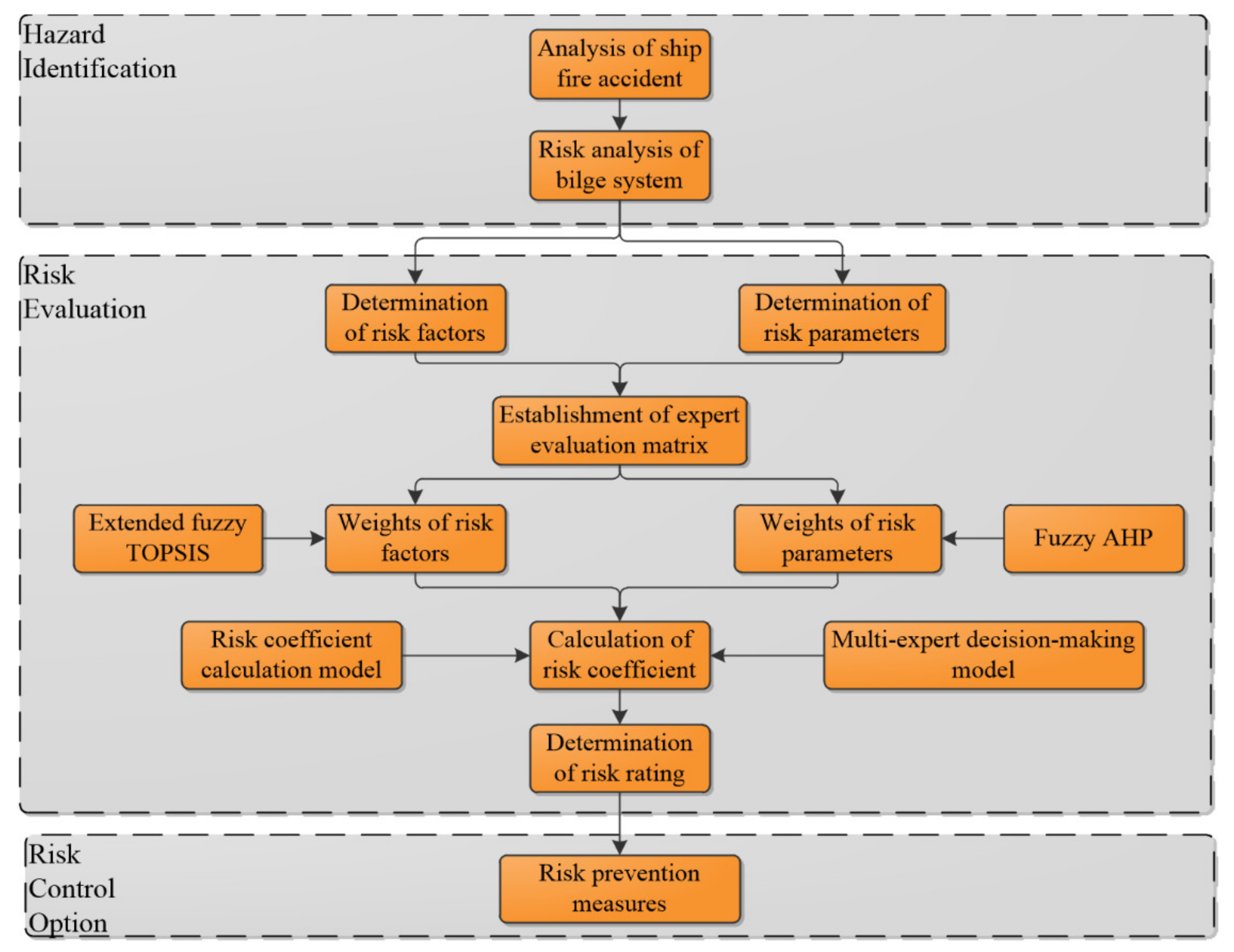
In 2002, IMO proposed the Formal Safety Assessment (FSA) process that comprises, for example, identification of hazards, risk evaluation, and risk control options [6]. Nevertheless, although FSA outlines the required steps, it does not offer a specific risk analysis tool for maritime stakeholders [7]. Such a lack of tools makes it necessary to rely on the knowledge and experience of experts when proposing an applicable failure risk assessment method.

1.2. Literature Review

Commonly used qualitative and quantitative evaluation methods are roughly divided into methods based on expert judgment (qualitative/quantitative), such as the Delphi method [8], bibliometric analysis methods such as bibliometric assessment [9], and mathematical analysis methods (quantitative), such as the Analytic Hierarchy Process (AHP) [10]. AHP is a method put forward by Saaty [11] that divides evaluation objectives into multiple levels and establishes mathematical models for their analysis. As a quantitative mathematical analysis method and a multi-criteria decision-making (MCDM) tool, AHP is practical, simple, and systematic and is widely applied in various disciplines, including engineering, economy, and management [12,13]. For example, Buckley [14] extended the hierarchical analysis to the case where experts can replace exact weights with fuzzy weights to rank the alternatives (i.e., criteria).

In the marine sector, Celik et al. [15] employed fuzzy AHP to select a suitable shipping registry for Turkish ship owners. Karahalios [16] combined AHP with fuzzy set theory to calculate and analyze the risk coefficients of three different ship types. To mitigate the shortcomings stemming from the process subjectivity and approximations of the results, AHP is frequently combined with the TOPSIS method [17]. TOPSIS is a commonly used method for MCDM problems that build on the idea that the best alternative should be the farthest from the negative ideal solution and the closest to the positive ideal solution [18,19]. Relating to fuzzy TOPSIS, Alarcin et al. [20] combined FST with TOPSIS to mitigate the TOPSIS’s deficiencies in dealing with fuzzy problems. Chen [21] extended TOPSIS to the fuzzy environment, calculating the distance between two triangular fuzzy numbers.

It is significant to aggregate opinions of several weighted decision-makers into group opinions in the group decision-making [22]. Expert competence (i.e., qualification level and decision-making capacity) and decision-making preferences (individual vs. group decision-making preference) impact the evaluation results. Thus, rather than weighting the experts equally when integrating their judgments, differences between them should be considered [23]. Nevertheless, the research on this aspect is relatively scarce. Chiclana et al. [24] discussed the Consistency-Induced Ordered Weighted Averaging operator for weighting the decision-making capacity of experts in group decision-making problems based on the consistency of their information sources. Aly and Vrana [25] regarded the experts’ knowledge, relevance, and experience as scoring indexes to determine the expert’s qualification level. However, the scoring index information is ambiguous and prone to overlap. Pythagorean fuzzy numbers [26] are incorporated with the individual decision-making preferences to represent experts’ evaluation accurately, capturing the fuzzy information in the decision-making process. Considering the group decision-making preference, Büyüközkan et al. [27] utilize each expert’s consensus degree coefficient to determine the expert weights. However, the proposed mathematical model omits the influence of experts’ individual decision-making preferences. Therefore, there is still a need for a comprehensive expert weight calculation model.

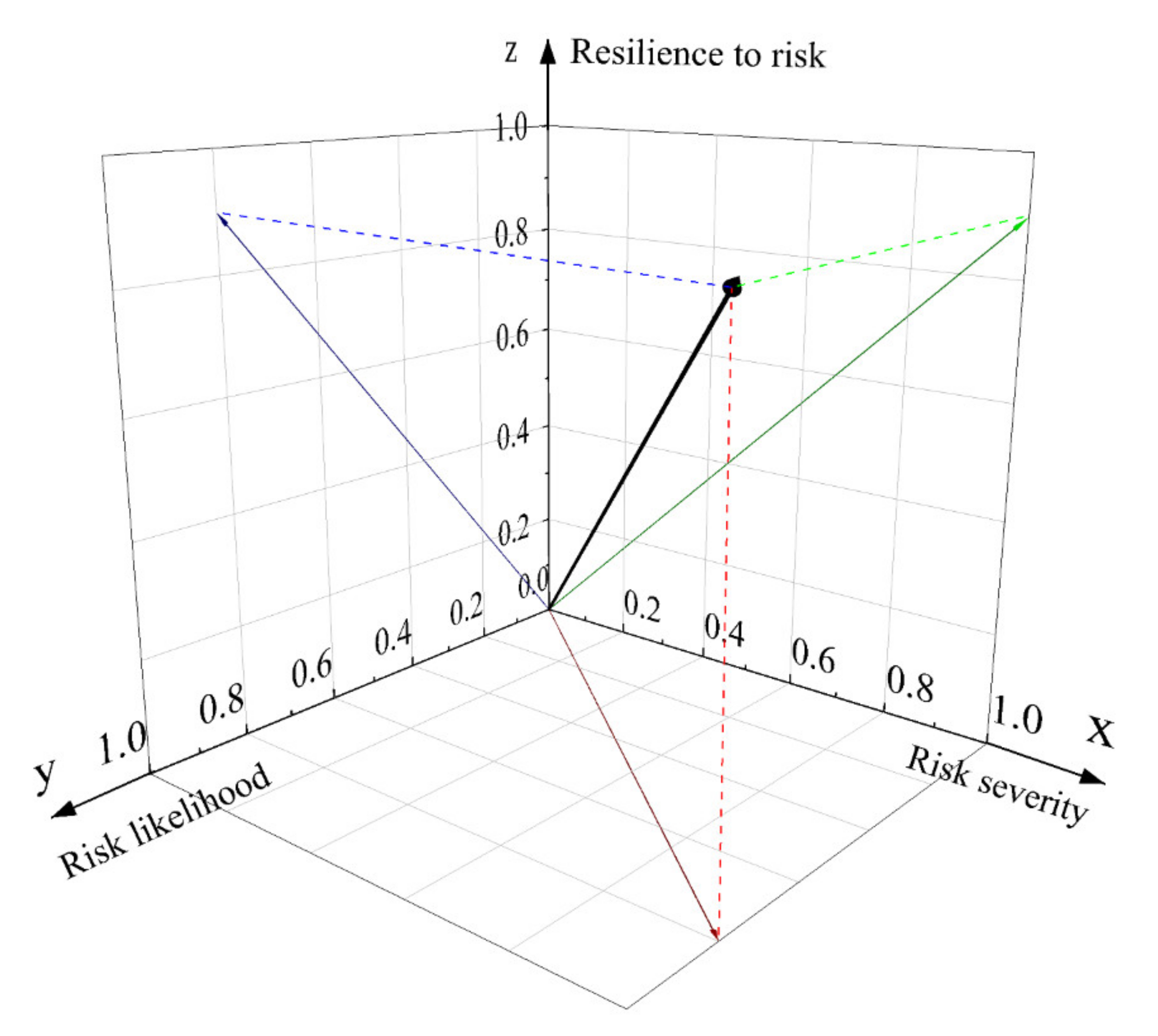
Another problem in risk evaluation is risk representation [28,29]. IMO defines risk as a combination of two risk parameters [30], as shown in Equation (1):

$$RC=O\times S$$

(1)

where the risk coefficient (denoted RC) is the quantitative risk representation, O is the risk likelihood rating, and S denotes the risk severity rating for the particular risk factor (i.e., criteria like the marine engines and pumps under fire accident conditions). Akyuz et al. [31] extended this notation by incorporating the capacity of detectability to risk (denoted D), and the RC can be calculated by taking the product of these three levels utilizing a numerical scale from 1 to 10, as shown in Equation (2):

$$RC=O\times S\times D,$$

(2)

where O, S, and D denote the level of risk factor’s likelihood, risk factor’s severity and the capacity of detectability to the risk, respectively. Additionally, O and S are benefit-type risk parameters and RC increases with a higher level of O and S. D is a cost-type risk parameter, which means a good capacity of detectability to risk may result in low level of D. Thus, RC decreases with a lower level of D (i.e., better capacity of detectability to the risk).

Anthony [32] and Montewka et al. [33] offered an improved risk coefficient calculation model, which transforms absolute risk coefficients into relative ones following Equation (3).

$$RC=w^o\times w^s,$$

(3)

where $w^o$ denotes the risk factor’s likelihood weight, and $w^s$ is the risk factor’s severity weight.

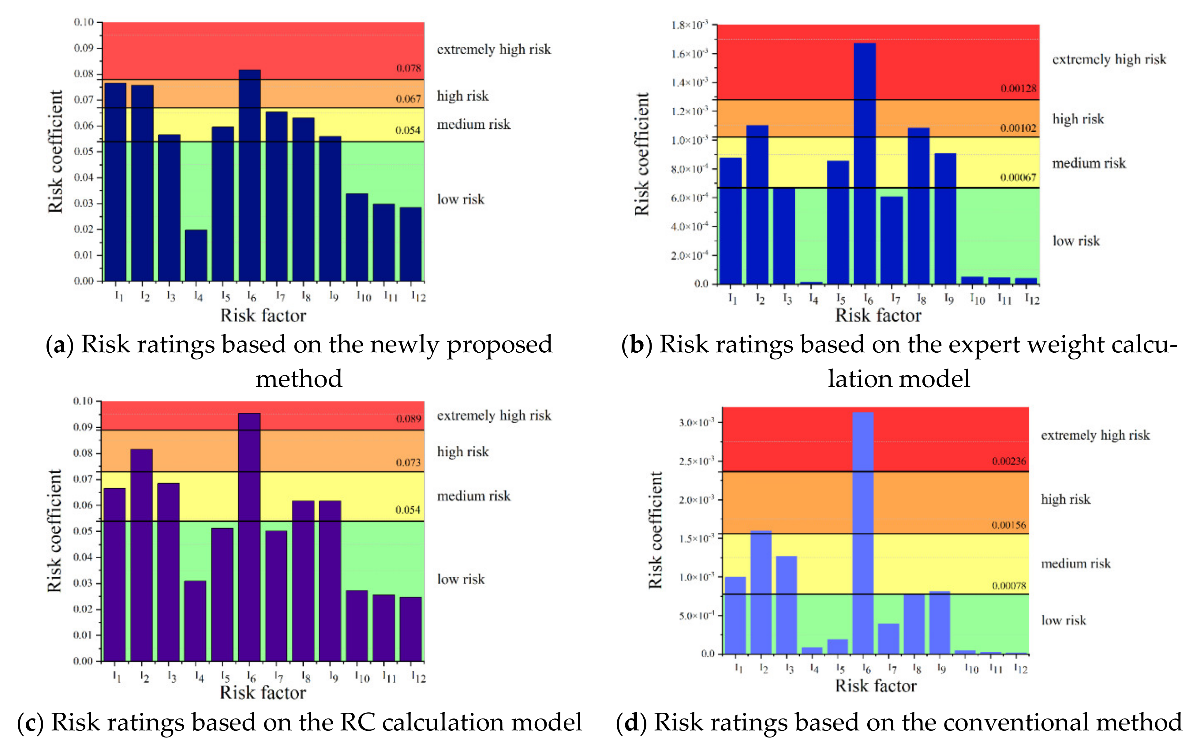
Risk coefficients determine the risk ratings. A review of risk matrices presented in [34] proposed a risk classification method based on a two-dimensional discrete risk matrix. Similarly, Hsu et al. [35] built on Equation (3) to propose a risk classification method based on a two-dimensional continuous risk matrix. However, there is little research related to a three-dimensional continuous risk matrix. Moreover, although a typical risk matrix provides a practical risk identification method, two problems arise when using the traditional RC calculation model that relies on multiplication.

• The same RC value implies that the risk factors’ actual ratings are identical. For example, consider a case where O, S, and D all equal two, and one where O = 4, S = 2, and D = 1. Following Equation (2), the two cases’ RCs are similar, and the risk ratings of the cases cannot be distinguished.
• Each risk parameter’s sensitivity to RC is the same. For example, let O, S, and D be 2, 2, 2, respectively in Equation (2). If O or S changes to 3, RC becomes 12. However, the influence of O, S, and D on risk rating should be different [7].

Resolving the listed problems requires a nonlinear aggregation of the risk parameters, with different weights assigned to distinct risk parameters. Thus, the risk coefficient calculation model is proposed.

In summary, the novelties and motivations of the proposed two methods for calculating the expert weight and risk coefficient can be summarized as follows:

• The expert weight calculation model comprehensively considers the differences in experts’ expertise levels (i.e., qualification level, decision-making capacity, and decision-making preference). Furthermore, there are shortcomings in some of existing expert weight calculation methods. Therefore, the weighted expert weight calculation model is proposed.
• A new RC calculation method is proposed to solve the list of two problems. The RC calculation model incorporates a nonlinear aggregation of the risk parameters, utilizing a three-dimensional continuous matrix that serves to determine the risk factors’ ratings. Additionally, the weights of different risk parameters are also considered.

The remainder of this paper is organized as follows. Section 2 introduces the preliminaries on the failure risk assessment for large luxury cruise ships’ bilge system. Section 3 describes the improved method for calculating the risk coefficients and determining the risk ratings. The application and discussion of the bilge system’s failure assessment on a Carnival Vista cruise ship example are presented in Section 4. Finally, Section 5 concludes the paper.

2. Preliminaries on Bilge System’s Failure Risk Assessment

Based on FSA, failure risk assessment for a large luxury cruise ship’s bilge system in case of fire is derived. In the order of hazard identification, risk evaluation and risk control option, the procedure of failure risk assessment is shown in Figure 1.

The purpose of hazard identification is to identify the potential high-risk areas of various ships under fire accident conditions, in order to advance corresponding risk prevention measures for elements of the bilge system located at high-risk areas. Hazard identification provides a reference for further analysis of high-risk areas for large cruise ships. Risk evaluation is a process of determining the predominant risk factors in the order of establishment of the risk matrix, calculation of risk coefficient, and determination of risk ratings. A risk matrix comprising risk factors and risk parameters is established to calculate the risk coefficient by quantifying the judgements of experts. The risk factors’ (e.g., bilge pump and bilge main pipe) weights are assessed using extended FTOPSIS, whereas the risk parameters (e.g., risk likelihood and risk severity) weights are assessed using FAHP. Additionally, the risk coefficient of each risk factor can be determined by the usage of two models. One is the risk coefficient model that incorporating a newly proposed method for calculating RC. The other is the multi-expert decision-making model that containing the expert weight calculation model. Finally, risk prevention measures are proposed based on the result of risk assessment. Further, attention should be paid to the predominant risk factors, especially these adjacent to potential high-risk areas.

2.1. Hazard Identification for Risk Analysis

This paper studies ship fire accidents from 2018 to 2020 reported by GISIS (Global Integrated Shipping Information System) [36]. Overall, 59 fire accidents are considered (most of which were serious or very serious), and their distribution based on accident locations is shown in Figure 2.

Compared with bulk carriers or container ships, there are few holds in large luxury cruise ships. Therefore, the bilge system’s components located in the engine room are critical for risk control measures. Additionally, attention should be paid to the bilge system adjacent to the areas that are easy to become the ignition source (i.e., fuel tank, cable, main engine, and boiler).

2.2. Decision-Making for the Evaluation

The kernel of the evaluation is the decision-making process of experts. According to the evaluation matrixes constructed by experts, fuzzy set theory, FAHP and extended FTOPSIS are applied to calculating RC, which is utilized to determine the risk factors’ ratings.

2.2.1. Evaluation Matrix Constructed by Experts

The expert evaluation matrix is constructed based on the risk factors and risk parameters [7]. Among them, the risk parameters that affect the risk ratings correspond to three phases [37]: before hazard (risk likelihood-O), during the hazardous event (resilience to risk-R), and after the hazard (risk severity-S). Based on the previous study [32,38], risk parameters and the corresponding risk ratings are shown in

Table 1. Risk parameters’ classification.

Risk Parameters	Linguistic Variables for the Risk Ratings	Description
O	Rare (level 1)	$0.0000\le O\le 0.0003$
	Unlikely (level 2)	$0.0003\le O\le 0.003$
	Possible (level 3)	$0.003\le O\le 0.03$
	Likely (level 4)	$0.03\le O\le 0.3$
	Almost certain (level 5)	$0.3\le O\le 1.0$
S	Insignificant (level 1)	No or only subsidiary damage, overall damage degree less than 20%
	Minor (level 2)	Slight subsidiary damage, overall damage degree 20–40%
	Moderate (level 3)	Serious subsidiary damage, overall damage degree 40%–60%
	Major (level 4)	Most of the system damaged, overall damage degree 60%–80%
	Catastrophe (level 5)	The system almost destroyed, overall damage degree more than 80%
R	Very poor (level 1)	Extreme long response time, almost no possibility of recovery
	Poor (level 2)	Long response time, low possibility of recovery
	Medium (level 3)	Timely response, moderate possibility of recovery
	Strong (level 4)	Quick response, high possibility of recovery
	Very strong (level 5)	Quick response, extremely high possibility of recovery

. Additionally, resilience to risk is a cost-type parameter, which means poor resilience to risk denotes high risk level.

2.2.2. Fuzzy Set for Decision-Making

Fuzzy set theory (FST) was first proposed by Zadeh in 1965. Fuzzy set $\tilde{Y}$ consists of an element set $x$ and membership function$\mu \left(x\right)$. A fuzzy set is commonly represented as a fuzzy triangular number (FTN) [23], i.e., $\tilde{Y}=\left(l, m, h\right)$, to simplify calculation and data analysis (see Figure 3). The FTN membership function is shown in Equation (4). The expert preference in decision-making is reflected by determining $l, m$, and $h$ values.

$$\mu \left(x\right)=\left\{\begin{array}{c}\left(x-l\right)/\left(m-l\right), l\le x\le m\\ \left(h-x\right)/\left(h-m\right), m\le x\le h\\ 0, otherwise\end{array}\right.,$$

(4)

2.2.3. Extended Fuzzy TOPSIS to Determine the Risk Factors’ Weights

FTOPSIS method is used to determining the ranks of risk factors, whereas extended FTOPSIS is employed to calculate risk factors’ weights for each risk parameter. Taking a single expert as an example, the steps of the extended fuzzy TOPSIS method are as follows.

Step 1. Establish the evaluation set.

Denote a risk factor set as $I=\left\{I_1, I_2,\dots ,I_n\right\}$ and a risk parameter set as $P=\left\{P_1, P_2,\dots ,P_S\right\}$.

Step 2. Construct the fuzzy evaluation matrix $\tilde{E}$:

$$\begin{array}{c}\begin{array}{cccc} P_1& P_2& \dots & P_S\end{array}\\ \tilde{E}={\left[{\tilde{x}}_{ij}\right]}_{n\times s}=\begin{array}{c}{I}_1\\ I_2\\ ⋮\\ I_n\end{array} \left[\begin{array}{cccc}{\tilde{x}}_{11}& {\tilde{x}}_{12}& \cdots & {\tilde{x}}_{1s}\\ {\tilde{x}}_{21}& {\tilde{x}}_{22}& \dots & {\tilde{x}}_{2s}\\ ⋮& ⋮& \ddots & ⋮\\ {\tilde{x}}_{n1}& {\tilde{x}}_{n2}& \cdots & {\tilde{x}}_{ns}\end{array}\right], \end{array}$$

(5)

where ${\tilde{x}}_{ij}=\left(l_{ij},m_{ij},h_{ij}\right)$.

Step 3. Standardize the fuzzy evaluation matrix ${\left[{\tilde{x}}_{ij}\right]}_{n\times s}$ (yielding ${\left[{\tilde{z}}_{ij}\right]}_{n\times s}$).

$$\begin{array}{c}{P}_1, P_2,\dots ,P_S\\ \tilde{Z}={\left[{\tilde{z}}_{ij}\right]}_{n\times s}=\left(C_1, C_2,\dots ,C_S\right),\end{array}$$

(6)

where ${\tilde{z}}_{ij}=\left(z_{ij}^{\left(l\right)},z_{ij}^{\left(m\right)},z_{ij}^{\left(h\right)}\right)$. If a particular risk parameter $P_j$ is a benefit-type parameter, the corresponding $C_j={\left({\tilde{z}}_{1j}^{+}, {\tilde{z}}_{2j}^{+}, \dots , {\tilde{z}}_{nj}^{+}\right)}^T$, ${\tilde{z}}_{ij}^{+}=\left(\frac{l_{ij}}{h_j^{+}},\frac{m_{ij}}{h_j^{+}},\frac{h_{ij}}{h_j^{+}}\right)$, $h_j^{+}=\underset{i}{\max }\left\{h_{ij}\right\}$. If $P_j$ is a cost-type parameter, the corresponding $C_j={\left({\tilde{z}}_{1j}^{-}, {\tilde{z}}_{2j}^{-}, \dots , {\tilde{z}}_{nj}^{-}\right)}^T$ ${\tilde{z}}_{ij}^{-}=\left(\frac{l_j^{+}}{l_{ij}},\frac{l_j^{+}}{m_{ij}},\frac{l_j^{+}}{h_{ij}}\right)$, $l_j^{+}=\underset{i}{\min }\left\{l_{ij}\right\}$.

Step 4. Calculate the fuzzy positive ideal solution ($FPI{S}_j$) and fuzzy negative ideal solution ($FNI{S}_j$) for each risk parameter following:

$$FPI{S}_j={\tilde{z}}_j^{+}=\left(\underset{i}{\max }\left\{{\tilde{z}}_{ij}\right\},\underset{i}{\max }\left\{{\tilde{z}}_{ij}\right\},\underset{i}{\max }\left\{{\tilde{z}}_{ij}\right\}\right),$$

(7)

$$FNI{S}_j={\tilde{z}}_j^{-}=\left(\underset{i}{\min }\left\{{\tilde{z}}_{ij}\right\},\underset{i}{\min }\left\{{\tilde{z}}_{ij}\right\},\underset{i}{\min }\left\{{\tilde{z}}_{ij}\right\}\right),$$

(8)

where $\underset{i}{\max }\left\{{\tilde{z}}_{ij}\right\}=\underset{i}{\max }\left\{z_{ij}^{\left(l\right)},z_{ij}^{\left(m\right)},z_{ij}^{\left(h\right)}\right\}$, $\underset{i}{\min }\left\{{\tilde{z}}_{ij}\right\}=\underset{i}{\min }\left\{z_{ij}^{\left(l\right)},z_{ij}^{\left(m\right)},z_{ij}^{\left(h\right)}\right\}$.

Step 5. Calculate each risk factor’s distance from $FPI{S}_j$ and $FPI{S}_j$.

$$D_i{}^{+}={\left(d_1^{+},d_2^{+},\dots ,d_n^{+}\right)}^T$$

(9)

$$D_i{}^{-}={\left(d_1^{-},d_2^{-},\dots ,d_n^{-}\right)}^T$$

(10)

where$d_i^{+}=d_v\left({\tilde{z}}_{ij},{\tilde{z}}_j^{+}\right)$ and $d_i^{-}=d_v\left({\tilde{z}}_{ij},{\tilde{z}}_j^{-}\right)$. Here, $d_v\left(\tilde{a},\tilde{b}\right)$ is the distance between $\tilde{a}$ and $\tilde{b}$, i.e.,

$$d_v\left(\tilde{a},\tilde{b}\right)=\sqrt{\frac{1}{3}{{\displaystyle \sum }}_{i=1}^3{\left(a_i-b_i\right)}^2}$$

(11)

$$\tilde{a}=\left(a_1,a_2,a_3\right)$$

(12)

$$\tilde{b}=\left(b_1,b_2,b_3\right)$$

(13)

Step 6. Calculate the closeness coefficient, which represents the distances from $FPI{S}_j$ and $FNI{S}_j$ simultaneously.

$$C_i={\left(c_1,c_2,\dots ,c_n\right)}^T$$

(14)

$$c_i=\frac{d_i^{-}}{d_i^{+}+d_i^{-}}$$

(15)

Step 7. Calculate the crisp weight of risk factors for each risk parameter [39].

$$W_i={\left(w_1,w_2,\dots ,w_n\right)}^T$$

(16)

$$w_i=\frac{c_i}{{{\displaystyle \sum }}_{i=1}^n{c}_i}$$

(17)

2.2.4. Fuzzy AHP to Determine the Risk Parameters’ Weights

Saaty incorporated FST and AHP into a fuzzy AHP (FAHP) theory, whose steps are as follows [23].

Step 1. Construct a fuzzy pairwise comparison matrix.

Equation (18) describes the construction of the pairwise comparison matrix, which requires the experts’ linguistic variables to be converted to FTNs.

$$F={\left[{\tilde{c}}_{ij}\right]}_{s\times s}=\left[\begin{array}{ccc}{\tilde{c}}_{11}& \cdots & {\tilde{c}}_{1s}\\ ⋮& \ddots & ⋮\\ {\tilde{c}}_{s1}& \cdots & {\tilde{c}}_{ss}\end{array}\right],$$

(18)

where ${\tilde{c}}_{ij}=\left(l_{ij},m_{ij},h_{ij}\right)$is a fuzzy set representing the comparison of importance between risk parameters $i$ and $j$. Note, $F$ is a reciprocal matrix, i.e., ${\tilde{c}}_{ij}>0$, ${\tilde{c}}_{ij}=1/{\tilde{c}}_{ji}$.

Using the language variables, experts compare the importance of risk parameters $i$ and $j$. By defining the fuzzy scale and applying TNFs, experts quantify the comparison results, determining $l$,$m$, and$h$ values for the particular ${\tilde{c}}_{ij}$. A typical five-level scale [40] is shown in

Table 2. Five-level scale and the corresponding language variables.

Language Variables	Ratings of a Five-Level Scale
Equal importance	1
Moderate importance	2
Significant importance	3
Very significant importance	4
Extremely significant importance	5

.

Step 2. Calculate the fuzzy weight.

Liu et al. [23] reviewed the pros and cons of methods for calculating fuzzy weights. Different methods should be introduced to different situations. For instance, mean method, eigenvector method, fuzzy programming, and Lambda–Max method are commonly utilized for the type-1 fuzzy sets (e.g., TNF). Nevertheless, Lambda–Max method is recognized as a better choice if the fuzzy weights are preferred and the fuzziness matter to the final results.

FTNs depend on the experts’ decision-making preferences, and the fuzziness greatly influences the calculation results. Thus, the Lambda–Max method [41] is used to calculate the fuzzy weight. The Lambda–Max method divides fuzzy pairwise comparison matrix $F$ (composed of FTNs) into three evaluation matrices, as shown in Equation (19):

$$F=\left\{\begin{array}{c}{\left[l_{ij}\right]}_{s\times s }, F=F_l\\ {\left[m_{ij}\right]}_{s\times s} , F=F_m\\ {\left[h_{ij}\right]}_{s\times s} , F=F_h\end{array}\right.$$

(19)

The three matrices’ maximum eigenvalues and corresponding eigenvectors are calculated following Equations (20) and (21):

$$F_l{w}_l={\lambda }_{max}{w}_l,$$

(20)

$$w_l={\left(w_{1l },w_{2l },\dots ,w_{sl }\right)}^T,$$

(21)

where ${\lambda }_{max}$denotes the maximum eigenvalues of $F_l$, and $w_l$ is the eigenvector corresponding to ${\lambda }_{max}$. Similarly,$w_m$ and $w_h$ can be represented as $w_m={\left(w_{1m },w_{2m },\dots ,w_{sm }\right)}^T$ and $w_h={\left(w_{1h },w_{2h },\dots ,w_{sh }\right)}^T$, respectively.

Let $K_l=\min \left\{\frac{w_{jm}}{w_{jl}}|1\le j\le s\right\}$ and $K_h=\max \left\{\frac{w_{jm}}{w_{jh}}|1\le j\le s\right\}$. Now, each risk parameter’s fuzzy weight is obtained as:

$${\tilde{w}}_j=\left(K_l{w}_{jl},w_{jm},K_h{w}_{jh}\right)=\left(w_{jl}^{*},w_{jm},w_{jh}^{*}\right).$$

(22)

Step 3. Calculate the crisp weight.

The crisp weight calculation is a defuzzification process. Within this process, Kar [42] incorporated the influence of the extreme values in FTNs on the results, as shown in Equations (23) and (24).

$$W_j={\left(w_1,w_2,\dots ,w_s\right)}^T$$

(23)

$$w_j=\frac{w_{jl}^{*}+2w_{jm}+w_{jh}^{*}}{4}$$

(24)

Step 4. Measure the consistency.

Since $F_l$ and $F_h$ are not reciprocal matrixes, the conventional consistency coefficient method [43] cannot be directly used for consistency measurement. Instead, the Centric Consistency Index (CCI) [44,45] is utilized (Equation (25)). If the derived index is smaller than the geometric consistency index (i.e.,$CCI\left(F\right)<\overline{GCI}$), the fuzzy matrix is considered consistent. The particular $\overline{GCI}$ values are given in

Table 3. Geometric consistency index values for different n values.

n	$\overline{\mathit{G}\mathit{C}\mathit{I}}$
3	0.31
4	0.35
>4	0.37

.

$$CCI\left(F\right)=\frac{2}{\left(n-1\right)·\left(n-2\right)}{{\displaystyle \sum }}_{i<j}(\log \left(\frac{a_{Lij}+a_{Mij}+a_{Uij}}{3}\right)-{\left(\log \left(\frac{w_{Li}+w_{Mi}+w_{Ui}}{3}\right)+\log \left(\frac{w_{Lj}+w_{Mj}+w_{Uj}}{3}\right)\right)}^2$$

(25)

3. Improved Calculation Model for Risk Ratings

The improved calculation model is utilized to minimize the issues encountered when using conventional methods for determining expert weights and risk coefficients, as discussed in Section 1.2. The expert weight calculation model comprehensively considers the differences in experts’ expertise levels (i.e., qualification level, decision-making capacity, and decision-making preference), the risk coefficient (RC) calculation model incorporates a three-dimensional continuous matrix and a new way to calculate RC.

3.1. Expert Weight Calculation Model

The experts’ evaluation results are commonly integrated using the FTOPSIS and FAHP processes. However, experts differ in qualification level and decision-making capacity. Moreover, the expert group decision-making preferences impact the evaluation results. A comprehensive risk factor’s weight is derived by combining the experts’ evaluations, as shown in Equations (26) and (27):

$$W_{fj}={{\displaystyle \sum }}_{t=1}^k{W}_j^{\left(t\right)}{\omega }_E^{\left(t\right)}=W_j^{\left(1\right)}·{\omega }_E^{\left(1\right)}+W_j^{\left(2\right)}·{\omega }_E^{\left(2\right)}+\dots +W_j^{\left(k\right)}·{\omega }_E^{\left(k\right)},$$

(26)

$${\omega }_E^{\left(t\right)}=\alpha {\omega }_q^{\left(t\right)}+\beta {\omega }_d^{\left(t\right)}+\gamma {\omega }_c^{\left(t\right)},$$

(27)

where $W_{fj}$ is the comprehensive weight of a particular risk factor, ${\omega }_E^{\left(t\right)}$ is the expert $E_t$’s weight derived from the expert’s qualification level weight (${\omega }_q^{\left(t\right)}$), the decision-making capacity weight (${\omega }_d^{\left(t\right)}$), and the relative degree of agreement (${\omega }_c^{\left(t\right)})$, $1\le t\le k$. The constants $\alpha , \beta , \gamma$ satisfy the equation $\alpha +\beta +\gamma =1$.

3.1.1. Experts’ Qualification Level

Due to the differences in the experts’ qualification levels, the experts’ judgment should be weighted differently. This paper proposes an expert sorting method (

Table 4. Expert scoring criteria.

Index	Categories	Score
Position	Closely related; Related; Unrelated to the evaluation object	5, 2, 1
Professional qualifications	Professor; Associate professor; Other	5, 2, 1
Education level	Doctor; Master; Other	5, 2, 1
Relevant achievements or experience	Major; Moderate; Minor	5, 2, 1
Judgment	Deep analysis; Reference data; Intuition	5, 2, 1
Entire working experience	Above 15 years; 5–15 years; below 5 years	5, 2, 1
Sailing experience	Above 12 years; 2–12 years; below 2 years	5, 2, 1

) that assigns each expert a qualification level weight.

However, the selection of expert scoring indexes is subjective, and an information overlap may exist between indexes. Thus, the principal component analysis (PCA) method [46] is employed to reduce the dimensions of the criteria and convert multiple variables into independent composite variables (i.e., principal components). The weights of principal components are calculated by variance contribution rate then the composite score is determined. The composite scores can reflect the comprehensive qualification level of each expert. Therefore, PCA was conducted using SPSS software [47] to integrate the indexes with major relevance and calculate the expert qualification level weights.

3.1.2. Experts’ Decision-Making Capacity

In AHP, the experts’ decision-making capacity can be determined using the variance $e_t^2$ of the expert’s pairwise comparison matrix F, i.e., following the so-called inverse judgment [48]. Here, $e_t^2$ represents the degree of inconsistencies in experts’ evaluations. The smaller the $e_t^2$, the stronger the experts’ decision-making capacity. However, if $F$ (derived following Equation (19)) is not a reciprocal matrix, the method cannot be directly used to calculate the experts’ decision-making capacity weights. This paper thus proposes a method for transforming the non-reciprocal matrix into a reciprocal one. The proposed method consists of the following steps.

Step 1. Perform defuzzification of the fuzzy pairwise comparison matrix $F$ from Equation (19) following Equations (28) and (29):

$$c_{ij}=\frac{l+2m+h}{4}$$

(28)

$$F^{*}={\left[c_{ij}\right]}_{s\times s}=\left[\begin{array}{ccc}{c}_{11}& \cdots & c_{1s}\\ ⋮& \ddots & ⋮\\ c_{s1}& \cdots & c_{ss}\end{array}\right]$$

(29)

Step 2. Convert the non-reciprocal matrix $F^{*}$ to reciprocal matrix $F^{\mathsf{\Delta }}$:

$$F^{\mathsf{\Delta }}={\left[{\mathrm{d}}_{ij}\right]}_{s\times s}=\left[\begin{array}{ccc}{d}_{11}& \cdots & d_{1s}\\ ⋮& \ddots & ⋮\\ d_{s1}& \cdots & d_{ss}\end{array}\right]$$

(30)

$${\mathrm{d}}_{ij}=\frac{1}{2}\left(c_{ij}+\frac{1}{c_{ji}}\right)$$

(31)

Step 3. Calculate the matrix A from the reciprocal matrix $F^{\mathsf{\Delta }}$:

$$A={\left[a_{ij}\right]}_{s\times s}$$

(32)

$$a_{ij}=\frac{b_{ij}}{\frac{1}{s}{{\displaystyle \sum }}_{j=1}^s{b}_{ij}}$$

(33)

$$b_{ij}=\frac{d_{ij}}{{{\displaystyle \sum }}_{i=1}^s{d}_{ij}}$$

(34)

Step 4. Calculate the derived matrix A’s variance ($e_t^2$):

$$e_t^2=\frac{1}{s^2}{{\displaystyle \sum }}_{i=1}^s{{\displaystyle \sum }}_{j=1}^s{\left(a_{ij}-1\right)}^2$$

(35)

Step 5. Determine the expert’s decision-making capacity:

$${\omega }_d^{\left(t\right)}=\frac{1/e_t^2}{{{\displaystyle \sum }}_{t=1}^k\left(1/e_t^2\right)}$$

(36)

3.1.3. Expert Group Decision-Making Preferences

The expert group decision-making preferences can be represented by the relative degree of agreement proposed by Chen [49]. In this method, individuals compromise with the whole decision-making group [50], following Equations (37)–(39). The greater the expert’s relative degree of agreement, the higher the expert’s weight. However, a fuzzy set used when calculating the relative degree of agreement has to be represented by a standard fuzzy number (i.e., $\left|m-l\right|=\left|h-m\right|$), and its fuzzy triangle is an isosceles triangle.

Let $E_t$ and $E_r$ denote two experts (out of k experts in a decision-making group). The degree of agreement between their evaluations is calculated as follows:

$$S\left({\tilde{C}}^{\left(t\right)},{\tilde{C}}^{\left(r\right)}\right)=1-\frac{\left|l^t-l^r\right|+\left|m^t-m^r\right|+\left|h^t-h^r\right|}{3}$$

(37)

$$A\left(E_t\right)=\frac{1}{k-1}{{\displaystyle \sum }}_{t=1, t\ne r}^{k}S\left({\tilde{C}}^{\left(t\right)},{\tilde{C}}^{\left(r\right)}\right)$$

(38)

$$RA\left(E_t\right)=\frac{A\left(E_t\right)}{{{\displaystyle \sum }}_{t=1}^{k}A\left(E_t\right)}$$

(39)

where $S\left({\tilde{C}}^{\left(t\right)},{\tilde{C}}^{\left(r\right)}\right)$ is the degree of evaluations’ agreement between experts$E_t$ and $E_r$, $A\left(E_t\right)$ is the average degree of agreement between expert $E_t$ and the decision-making group, and $RA\left(E_t\right)$ is expert $E_t$’s relative degree of agreement. ${\tilde{C}}^{\left(t\right)}=\left(l^t,m^t,h^t\right)$ and ${\tilde{C}}^{\left(r\right)}=\left(l^r,m^r,h^r\right)$ are standardized triangle fuzzy numbers, and $0\le l^t\le m^t\le h^t\le 1, 0\le l^r\le m^r\le h^r\le 1$.

Two special cases for FTNs emerge when considering the expert preferences in the decision-making process and calculating expert $E_t$’s relative degree of agreement (see Figure 4).

The red triangle in Figure 4a represents expert $E_t$’s FTN, whereas the blue triangle is expert $E_r$’s FTN. Experts $E_t$and $E_r$ are not in complete agreement. However, if Equation (37) is utilized, experts $E_t$ and $E_r$ almost reach a consensus. In the case depicted in Figure 4b, from $E_t$’s perspective, experts $E_r$ and $E_t$ do not perfectly agree, but $E_r$ perceives that a high level of agreement. The reason for such a discrepancy is as follows. Suppose there are nonempty sets A and B, $A\subseteq B$, $A\ne B$. If $x\in A$, then $x\in B$. Still, $x\in B$ does not necessarily mean $x\in A$. Nevertheless, if Equation (37) is used to calculate the degree of agreement, experts $E_t$ and $E_r$ reach a consensus, i.e., $S\left({\tilde{C}}^{\left(t\right)},{\tilde{C}}^{\left(r\right)}\right)=S\left({\tilde{C}}^{\left(r\right)},{\tilde{C}}^{\left(t\right)}\right)$.

To eliminate such inconsistencies, Equation (37) is redefined, resulting in Equations (40) and (41):

$$S_{\mathsf{\Delta }}\left({\tilde{C}}^{\left(t\right)},{\tilde{C}}^{\left(r\right)}\right)=\frac{S_{t\mathsf{\Lambda }r}}{S_t},$$

(40)

$$S_{\mathsf{\Delta }}\left({\tilde{C}}^{\left(r\right)},{\tilde{C}}^{\left(t\right)}\right)=\frac{S_{t\mathsf{\Lambda }r}}{S_r},$$

(41)

where $S_{t\mathsf{\Lambda }r}$ is the intersection area of two triangles, $S_t$ is the area of the triangle representing $E_t$’s evaluation, and $S_r$ is the area of the triangle representing $E_r$’s evaluation. The membership function $\mu \left(x\right)$ of ${\tilde{C}}^{\left(t\right)}$ or ${\tilde{C}}^{\left(r\right)}$ is a triangle whose height equals one [45,51].

3.2. Risk Coefficient Calculation Model

Based on the risk coefficient (RC) values, this work uses a continuous risk matrix to categorize the hazards into four ratings, namely “low risk”, “medium risk”, “high risk”, and “extremely high risk”. According to the three risk parameters in Table 1 (likelihood, severity, and resilience), a three-dimensional continuous risk matrix is constructed (see Figure 5). In Figure 5, $x$-axis represents the risk severity, $y$-axis is the risk likelihood, and $z$-axis is the resilience to risk.

Let $\overrightarrow{I_i}=\left(x_i,y_i,z_i\right)$ denote a vector where $x_i$ is the risk factor’s severity weight, $y_i$ is the risk factor’s likelihood weight, and $z_i$ is the risk factor’s resilience weight. Risk coefficient (RC) can be redefined as shown in Equation (42):

$$R{C}_i=\sqrt{{\left(W_{f1}{x}_i\right)}^2+{\left(W_{f2}{y}_i\right)}^2+{\left(W{f}_3{z}_i\right)}^2},$$

(42)

$$W_f={\left(W_{f1}, W_{f2}, W_{f3}\right)}^T,$$

(43)

where $R{C}_i$ is the risk coefficient of a particular risk factor, and $W_f$ denotes the comprehensive weights of the risk parameters—in particular,$W_{f1}$ is the risk factor’s severity weight, $W_{f2}$ is the likelihood weight, and $W_{f3}$ is the resilience weight.

Now, the mean value method [35] can be used to classify the risk factors, as shown in Equation (44):

$$A{v}_1=\frac{{{\displaystyle \sum }}_{i=1}^{n}R{C}_i}{n}$$

(44)

Let $n_1$ denote the number of risk factors whose coefficients satisfy the condition $R{C}_i<A{v}_1$, and $n_2$ the number of risk factors that meet the $R{C}_i\ge A{v}_1$ condition, $n_1+n_2=n$. Then, $n_1$ risk factors can be categorized as low risk. The average risk coefficient of the remaining risk factors yields $A{v}_2$, and $n_2$ risk factors can be categorized into two groups. In the first group, there are $n_{21}$ risk factors meeting the $R{C}_i<A{v}_2$ condition. These factors are categorized as medium risk. In the second group, there are $n_{22}$ remaining risk factors satisfying $R{C}_i\ge A{v}_2 (n_{21}+n_{22}=n_2$), which are then used to calculate $A{v}_3$ serving as a boundary between high and extremely high risks.

4. Case Study and Discussion

In the process of Vista cruise ship design, risk assessment can provide references for its bilge system’s arrangements that can enhance the Vista cruise ship’s probability of SRtP. This section applies the proposed method to determine the predominant risk factors (i.e., factors falling into the medium-risk or higher category) and corresponding risk control measures for the Vista cruise ship’s bilge system. The Vista cruise ship’s principal dimensions are shown in

Table 5. The Vista cruise ship’s principal dimensions.

Principal Dimensions	Value	Unit
Overall Length/Length between Perpendiculars	323.6/287.1	m
Molded Depth	11.4	m
Molded Breadth	37.2	m
Maximum Draft	8.5	m
Gross Tonnage	133500.0	GT

.

To meet the SOLAS requirements regarding SRtP, all fire accidents are considered serious (i.e., at least one person died or the ship is seriously damaged) [52].

4.1. The Evaluation Procedure

This section elaborates the failure assessment based on the proposed method (as shown in Figure 1). The definite processes are as follows.

4.1.1. Expert’s Evaluation Matrix Establishment

As noted in Section 2.2.1, the expert evaluation matrix consists of risk factors and risk parameters.

Table 6. Risk factors of the VISTA cruise ship’s bilge system.

Criteria	Sub-Criteria	Symbol
Power machinery	Oily bilge pump (reciprocating pump)	I1
	Rule bilge pump (centrifugal pump)	I2
	Spare pump (screw pump)	I3
Facility	Bilge holding tank	I4
	Electric control of bilge system	I5
Pipeline	Bilge main pipe	I6
	Bilge branch pipe	I7
	Valve	I8
	Other piping accessories	I9
Measuring instrument	Level gauge	I10
	Pressure gauge	I11
	Flow gauge	I12

lists the risk factors, whereas the risk parameters are shown in Table 1 (i.e., risk likelihood, severity, and resilience).

Evaluations from ten experts were collected. As an example, expert $E_1$’s fuzzy evaluation matrix is shown in

Table 7. Expert $E_1$’s evaluation matrix.

	O	S	R
I1	(1,2,3)	(2,3,4)	(1,1,2)
I2	(2,2,3)	(3,4,4)	(1,1,2)
I2	(2,3,3)	(3,4,5)	(1,2,2)
I4	(1,1,2)	(1,2,2)	(1,2,3)
I5	(1,2,2)	(2,3,4)	(2,3,3)
I6	(3,3,4)	(3,4,5)	(1,1,2)
I7	(2,3,4)	(3,3,4)	(2,3,3)
I8	(3,3,4)	(2,3,4)	(2,2,3)
I9	(3,4,4)	(2,3,3)	(2,2,3)
I10	(2,2,3)	(1,2,2)	(3,3,4)
I11	(2,3,3)	(1,1,2)	(3,4,4)
I12	(2,3,3)	(1,1,2)	(3,4,4)

. Experts assess the risk likelihood, the resilience to risk and the risk severity for each risk factor and quantify the judgements of experts. The results can be expressed as a fuzzy number like (a, b, c), a and c are the minimum and maximum value, respectively, whereas b is the expected value. Likewise, fuzzy evaluation matrices of the other experts were obtained.

4.1.2. Risk Coefficient Calculation

Step 1. Determining the risk parameter weights.

The risk parameters’ weights were determined using FAHP. Expert $E_1$’s fuzzy pairwise comparison matrix is shown in

Table 8. Fuzzy pairwise comparison matrix for expert $E_1$.

	O	S	R
O	(1,1,1)	(1/5,1/4,1/2)	(1,2,3)
S	(2,4,5)	(1,1,1)	(3,5,5)
R	(1/3,1/2,1)	(1/5,1/5,1/3)	(1,1,1)

. A similar procedure is used to derive fuzzy pairwise comparison matrices of other experts.

The risk parameters’ fuzzy weights and crisp weights were obtained using Equations (18)–(24) and are shown in

Table 9. Risk parameters’ fuzzy and crisp weights.

Risk Parameter	Fuzzy Weight	Crisp Weight (Standardized)
O	(0.227, 0.277, 0.366)	0.212
S	(0.703, 0.9471, 0.947)	0.657
R	(0.162, 0.162,0.220)	0.131

. The derived CCI calculated as specified in Equation (25) equals 0.052. Since $CCI=0.052<0.31$, the fuzzy pairwise comparison matrix passes the consistency measurement.

The risk parameters’ comprehensive weights were obtained by integrating the evaluations of ten experts. However, as discussed in previous sections, the experts’ qualifications, decision-making capacities, and decision-making preferences must be considered. The experts’ qualification levels were determined using the expert scoring system (Table 4). PCA for each scoring index was performed to obtain the composite score (i.e., comprehensive score coefficient) [46] of a particular expert. Thus, ten experts were rated based on the comprehensive score coefficient, and the experts’ qualification level weights shown in

Table 10. Experts’ qualification level weights.

	E1	E2	E3	E4	E5	E6	E7	E8	E9	E10
Comprehensive score coefficient	2.996	3.858	3.897	2.43	1.429	3.822	3.117	1.481	2.43	0.323
Expert weights	0.111	0.143	0.144	0.09	0.053	0.141	0.115	0.055	0.09	0.058

.

The expert decision-making capacity was determined using the derived matrix’s variance.

Table 11. Experts’ decision-making capacity weights.

	E1	E2	E3	E4	E5	E6	E7	E8	E9	E10
Derived matrix variance	0.015	0.012	0.011	0.024	0.035	0.011	0.024	0.033	0.023	0.038
Expert weight	0.128	0.149	0.168	0.078	0.054	0.168	0.076	0.057	0.080	0.048

shows the ten experts’ decision-making capacity weights derived using Equations (28)–(36).

The expert group decision-making preferences are represented by the relative degree of agreement. Following Equations (38)–(41), the experts’ relative degrees of the agreement were obtained (

Table 12. Experts’ relative degree of agreement for the calculation of risk parameters’ weights.

	E1	E2	E3	E4	E5	E6	E7	E8	E9	E10
Expert weight	0.149	0.134	0.122	0.092	0.087	0.201	0.067	0.054	0.044	0.050

).

Selecting$\alpha =0.5, \beta =0.3,\gamma =0.2$ in the Equation (27) yields the comprehensive risk parameters’ weights $W=\left(0.267, 0.498, 0.235\right)$.

Step 2: Determining the risk factor weights

The risk factors’ weights were calculated using the extended FTOPSIS applied to the expert evaluation matrix shown in Table 7. Resilience to risk served as a cost indicator. Thus, the worse the resilience to risk, the higher the resilience weights. The risk factor weights for expert $E_1$ are shown in

Table 13. Risk factors’ weights derived for expert $E_1$.

Risk Factors	I1	I2	I3	I4	I5	I6	I7	I8	I9	I10	I11	I12
Likelihood weight	0.058	0.070	0.086	0.027	0.040	0.117	0.098	0.116	0.129	0.086	0.086	0.086
Severity weight	0.107	0.142	0.116	0.027	0.099	0.166	0.083	0.103	0.098	0.026	0.019	0.014
Resilience weight	0.161	0.161	0.127	0.115	0.048	0.161	0.048	0.064	0.064	0.021	0.015	0.015

. Similarly, the risk factor weights for other experts can be calculated using their evaluation matrices.

Similar to the risk parameters case, the comprehensive risk factors’ weights were obtained by integrating the evaluations of ten experts. The experts’ qualification level weights are consistent with Table 10. Each expert’s relative degree of agreement is shown in

Table 14. Experts’ relative degree of agreement for the risk factors weights’ calculation.

	E1	E2	E3	E4	E5	E6	E7	E8	E9	E10
Expert weight	0.109	0.164	0.171	0.072	0.088	0.131	0.067	0.084	0.054	0.060

.

The constants$\alpha =0.5, \beta =0.3,\gamma =0.2$ were utilized in Equation (27), and the derived comprehensive risk factor weights are shown in

Table 15. Comprehensive risk factors’ weights.

Risk Factors	I1	I2	I3	I4	I5	I6	I7	I8	I9	I10	I11	I12
Likelihood weight	0.044	0.051	0.066	0.013	0.089	0.068	0.128	0.123	0.119	0.106	0.099	0.094
Severity weight	0.135	0.126	0.096	0.037	0.100	0.135	0.110	0.100	0.081	0.037	0.026	0.026
Resilience weight	0.147	0.171	0.105	0.027	0.096	0.182	0.043	0.088	0.094	0.013	0.018	0.016

.

Step 3. Calculating the risk coefficients (RC)

The risk factors’ risk coefficients were calculated following Equation (42) and shown in

Table 16. Risk coefficient for risk factors.

Risk Factors	I1	I2	I3	I4	I5	I6	I7	I8	I9	I10	I11	I12
Risk coefficient	0.077	0.076	0.057	0.020	0.060	0.082	0.066	0.063	0.056	0.034	0.030	0.029

. It shows that the main bilge pump’s (I₆) risk coefficient is the highest, highlighting the main bilge pump as one of the critical risk factors.

4.2. Determination of Risk Ratings and Sensitivity Analysis

The mean value method, described with Equation (44), was utilized to determine each risk factor’s risk rating (Figure 6). The maximum threshold in Figure 6 are the $A{v}_3$, whereas the minimum threshold is $A{v}_1$. Additionally, $A{v}_2$ is the threshold between high risk and medium risk. Incorporating the expert weight calculation model (i.e., Equation (27)) and the risk coefficient calculation model (i.e., Equation (42)) yields the risk rating shown in Figure 6a. When the expert weights are considered (i.e., Equation (27)), and the conventional risk coefficient calculation method is utilized (i.e., Equation (3)), the risk rating shown in Figure 6b is obtained. Omitting the expert weights (i.e., regarding the expert weights as equal) and using the risk coefficient calculation model results in the risk rating shown in Figure 6c. Finally, disregarding both the expert weight (i.e., regarding the expert weights as equal) and the risk coefficient calculation model (i.e., employing the conventional method) results in the risk ratings shown in Figure 6d.

The sensitivity analysis was conducted with respect to two different control strategies: the expert’s weights and the risk coefficient calculation model.

To comparatively analyze the influence of expert weights, Equation (42) was utilized to calculate RCs in Figure 6a,c, but the method depicted in Figure 6a considered the expert weights, while the other one did not. Two high-risk factors (I₁ and I₂) are identified in Figure 6a, while the method corresponding to Figure 6c detected only one high-risk factor (I₂). Similar conclusions could be drawn by comparing Figure 6b,d. Both methods highlight I₂ as a high-risk factor, but the method using the expert weights (Figure 6b) detected additional factors. Further, all of the methods recognize I₆ as the highest-risk factor. These results demonstrate the utility of the expert weight calculation model to identify high-risk factors, revealing its moderate influence on the evaluation results.

In the comparative analysis of the impact of the risk coefficient calculation model, one should contrast Figure 6a,b. Both methods consider the expert weights when calculating RC, but only Figure 6a uses the RC calculation model (i.e., Equation (42)). Although the influence of the risk coefficient calculation model on the identification of high-risk factors is not pronounced, Figure 6a enables the identification of eight predominant risk factors, of which five are medium-risk (I₃, I₅, I₇, I₈, I₉). In contrast, Figure 6b identifies only six predominant risk factors, three of which are classified as medium-risk factors (I₁, I₅, I₉). Similar conclusions can be drawn by comparing Figure 6c,d. These results prove the proposed risk coefficient calculation model’s influence on the evaluation results.

In summary, the proposed models are beneficial for the identification of predominant risk factors. Several issues are identified compare to existing models. The comparison of Figure 6a,d highlights the significant improvement in the identification of predominant risk factors achieved by combining the expert weight calculation model and the risk coefficient calculation model. There are seven risk factors (I₄, I₅, I₇, I₈, I₁₀, I₁₁, I₁₂,) that are low-risk in Figure 6d, while only four are low-risk (I₄, I₁₀, I₁₁, I₁₂) in Figure 6a. Therefore, the bilge branch line, valve, and electric control of the bilge system are also significant objects for the risk control option. In addition, the proposed models also identify a critical issue (i.e., another high-risk factor, I₁). Furthermore, the influence of the expert weight calculation model on the evaluation results is not as pronounced as that of the risk coefficient calculation model in identifying medium-risk factors. However, the opposite is true when identifying high-risk factors.

4.3. Risk Control Option

The risk evaluation presented in the previous sections showed that the risk rating of the main bilge pipe is the highest of all the risk factors. Thus, it is preferred to design the prevention measures for the bilge main located at the high-risk area (Figure 2) or near the area where ignitions are likely to start. Bilge pumps with high-risk ratings and poor resilience to risks should be distributed over different MVZs in an alternating fashion. The risk control measures for the VISTA cruise ship’s bilge system are as follows [53] and Figure 7, Figure 8 and Figure 9 provide the practical solutions to the original bilge system for designers.

• Distributed power machinery: There are six MVZs in the VISTA cruise ship. Therefore, four bilge pumps connected to the bilge main are separated into different MVZs. Emergency bilge pump and rule bilge pump are located at MVZ2 and MVZ3, respectively. Moreover, No. 1 and No. 2 bilge/ballast pumps are located at MVZ1 and MVZ6 on the upper deck of the emergency bilge pump, respectively (see Figure 7). The oil bilge pump is located at MVZ4 (Figure 8). The spare pump is arranged in MVZ6 on Deck 4 (see Figure 9).

2.

Redundancy: For the VISTA cruise ship’s rule bilge system, the redundant design is necessary to prevent the bilge main from being damaged and losing control of the bow and stern due to a fire accident. Redundant bilge main is fitted above the fuel tank at the stern and the end of the pipe tunnel at the bow, respectively (see Figure 9). However, the redundant bilge main cannot be fitted below the original bilge main.

3.

Fire-resistant pipe: Of the rule bilge system elements, the bilge main is located at the engine room (high-risk area), at the bow (high-risk area with fuel tank), and the stern should be fire-resistant (see Figure 7 and Figure 9). The oily bilge system’s No. 1 oily bilge pipe is used for daily collecting oily bilge water, and No. 2 oily bilge pipe serves solely for collecting oily bilge water from the compartments with important equipment. Therefore, the bilge pipe for the overboard discharge and No. 1 oily bilge pipe should be fire-resistant to ensure the basic emission function in the event of serious fire accidents (see Figure 8).

4.

Quarantine: Bilge main is fitted with isolation valves (e.g., butterfly valves) on both sides of watertight bulkheads (see Figure 7). When a fire accident occurs in one watertight compartment, the bilge main’s isolation valve can be used to prevent the bilge system outside of the damaged area from being affected. Moreover, the isolation valve must be easily accessible.

5. Conclusions

This paper improves the conventional failure risk assessment method for a cruise ship’s bilge system by incorporating the expert weight calculation model and the risk coefficient calculation model. The proposed method has several advantages. First, the method successfully handles the risk ratings’ categorization. Second, it enables systematic derivation of the decision-maker weights. Finally, each risk factor’s comprehensive weight stems from the effective integration of experts’ evaluations.

The case study results demonstrate the proposed method’s usefulness for the VISTA cruise ship’s bilge system risk assessment and analysis for severe fire accident scenarios. The expert weight calculation model obtains the decision-maker weights while accounting for their qualification level, decision-making capacity, and group decision preference. The risk coefficient calculation model identified the predominant risk factors, i.e., bilge main and bilge pumps. The sensitivity analysis demonstrated that the proposed models are beneficial for the identification of the predominant risk factors. Therefore, the proposed calculation models form an effective tool to determine the risk ratings for the bilge system in the VISTA cruise ship. Based on these findings, countermeasures are put forward to enhance the large luxury cruise ships’ probability of SRtP.

However, it should be mentioned that the expert weight calculation model should be used with caution if there are few relatively high-level experts in a group of experts, which makes the evaluation results of high-level experts not predominant enough. Further, future studies should explore the influence of the variation in parameters $\alpha ,\beta ,\gamma$ in Equation (27) on the evaluation results. The cost is rarely considered in the context of large luxury cruise ships. Thus, benefits analysis in FSA should be addressed in the future when the costs gain more attention from marine stakeholders. Finally, hazard identification of various ships provides only a reference for further analysis of fire accidents on large cruise ships. Future studies about ship fire accidents should focus on cruise ships due to its limited data.

References

1. Lyu, J.; Hu, L.; Hung, K.; Mao, Z.X. Assessing servicescape of cruise tourism: The perception of Chinese tourists. Int. J. Contemp. Hosp. Manag. 2017, 29, 2556–2572. [Google Scholar] [CrossRef]
2. Wang, P.; Wang, F.; Chen, Z. Investigation on aerodynamic performance of luxury cruise ship. Ocean Eng. 2020, 213, 107790. [Google Scholar] [CrossRef]
3. Sarıalioğlu, S.; Uğurlu, Ö.; Aydın, M.; Vardar, B.; Wang, J. A hybrid model for human-factor analysis of engine-room fires on ships: HFACS-PV&FFTA. Ocean Eng. 2020, 217, 107992. [Google Scholar]
4. Lloyd’s Register of Shipping. Rules and Regulations for the Classification of Ships; Lloyd’s Register of Shipping: London, UK, 2018. [Google Scholar]
5. International Maritime Organization. International Convention for Safety of Life at Sea, (SOLAS); International Maritime Organization: London, UK, 2021. [Google Scholar]
6. Zhang, D.; Yan, X.P.; Yang, Z.L.; Wall, A.; Wang, J. Incorporation of formal safety assessment and Bayesian network in navigational risk estimation of the Yangtze River. Reliab. Eng. Syst. Saf. 2013, 118, 93–105. [Google Scholar] [CrossRef]
7. Gul, M.; Celik, E.; Akyuz, E. A hybrid risk-based approach for maritime applications: The case of ballast tank maintenance. Hum. Ecol. Risk Assess. 2017, 23, 1389–1403. [Google Scholar] [CrossRef]
8. Geist, M.R. Using the Delphi method to engage stakeholders: A comparison of two studies. Eval. Program. Plann. 2010, 33, 147–154. [Google Scholar] [CrossRef]
9. Iivari, J. Expert evaluation vs bibliometric evaluation: Experiences from Finland. Eur. J. Inf. Syst. 2008, 17, 169–173. [Google Scholar] [CrossRef]
10. Demirel, H.; Balin, A.; Celik, E.; Alarçin, F. A fuzzy AHP and electre method for selecting stabilizing device in ship industry. Brodogradnja 2018, 69, 61–77. [Google Scholar] [CrossRef]
11. Saaty, T.L. The Analytical Hierarchy Process; McGraw-Hill International: New York, NY, USA, 1980. [Google Scholar]
12. Akyildiz, H.; Mentes, A. An integrated risk assessment based on uncertainty analysis for cargo vessel safety. Saf. Sci. 2017, 92, 34–43. [Google Scholar] [CrossRef]
13. Mardani, A.; Jusoh, A.; Zavadskas, E.K. Fuzzy multiple criteria decision-making techniques and applications–Two decades review from 1994 to 2014. Expert Syst. Appl. 2015, 42, 4126–4148. [Google Scholar] [CrossRef]
14. Buckley, J.J. Fuzzy hierarchical analysis. Fuzzy Sets Syst. 1985, 17, 233–247. [Google Scholar] [CrossRef]
15. Celik, M.; Deha Er, I.; Fahri Ozok, A. Application of fuzzy extended AHP methodology on shipping registry selection: The case of Turkish maritime industry. Expert Syst. Appl. 2009, 36, 190–198. [Google Scholar] [CrossRef]
16. Karahalios, H. The severity of shipboard communication failures in maritime emergencies: A risk management approach. Int. J. Disaster Risk Reduct. 2018, 28, 1–9. [Google Scholar] [CrossRef]
17. Ertuğrul, İ.; Karakaşoğlu, N. Comparison of fuzzy AHP and fuzzy TOPSIS methods for facility location selection. Int. J. Adv. Manuf. Technol. 2008, 39, 783–795. [Google Scholar] [CrossRef]
18. Celik, E.; Akyuz, E. An interval type-2 fuzzy AHP and TOPSIS methods for decision-making problems in maritime transportation engineering: The case of ship loader. Ocean Eng. 2018, 155, 371–381. [Google Scholar] [CrossRef]
19. Karahalios, H. The application of the AHP-TOPSIS for evaluating ballast water treatment systems by ship operators. Transp. Res. D Transp. Environ. 2017, 52, 172–184. [Google Scholar] [CrossRef]
20. Alarcin, F.; Balin, A.; Demirel, H.D. Fuzzy AHP and Fuzzy TOPSIS integrated hybrid method for auxiliary systems of ship main engines. J. Mar. Eng. Technol. 2014, 13, 3–11. [Google Scholar]
21. Chen, C. Extensions of the TOPSIS for group decision-making under fuzzy environment. Fuzzy Sets Syst. 2000, 114, 1–9. [Google Scholar] [CrossRef]
22. Petra, G.; Lidija, Z.S. Evaluation of several approaches for deriving weights in fuzzy group analytic hierarchy process. J. Decis. Syst. 2018, 27 (Suppl. 1), 217–226. [Google Scholar]
23. Liu, Y.; Eckert, C.M.; Earl, C. A review of fuzzy AHP methods for decision-making with subjective judgements. Expert Syst. Appl. 2020, 161, 113738. [Google Scholar] [CrossRef]
24. Chiclana, F.; Herrera-Viedma, E.; Herrera, F.; Alonso, S. Some induced ordered weighted averaging operators and their use for solving group decision-making problems based on fuzzy preference relations. Eur. J. Oper. Res. 2007, 182, 383–399. [Google Scholar] [CrossRef]
25. Aly, S.; Vrana, I. Evaluating the knowledge, relevance and experience of expert decision makers utilizing the Fuzzy-AHP. Agric. Econ. 2008, 54, 529–535. [Google Scholar] [CrossRef] [Green Version]
26. Tian, C.; Peng, J.J.; Zhang, W.Y.; Zhang, S.; Wang, J.Q. Tourism environmental impact assessment based on improved AHP and picture fuzzy promethee li Methods. Technol. Econ. Dev. Econ. 2019, 26, 355–378. [Google Scholar] [CrossRef]
27. Büyüközkan, G.; Karabulut, Y.; Arsenyan, J. RFID service provider selection: An integrated fuzzy MCDM approach. Measurement 2017, 112, 88–98. [Google Scholar] [CrossRef]
28. Sun, M.L.; Zhang, Z.Y.; Gang, L.H. Uncertainty analysis of the estimated risk in formal safety assessment. Sustainability 2018, 10, 321. [Google Scholar] [CrossRef] [Green Version]
29. Harilaos, N. Formal Safety Assessment:an updated review. J. Mar. Sci. Technol. 2012, 17, 390–402. [Google Scholar]
30. International Maritime Organization. Revised Guidelines for Formal Safety Assessment (FSA) for Use in the IMO Rule-Making Process, 2018. MSC-MEPC.2/Circ.12/Rev.2. Available online: http://shippingregs.org/ (accessed on 25 March 2021).
31. Akyuz, E.; Akgun, I.; Celik, M. A fuzzy failure mode and effects approach to analyse concentrated inspection campaigns on board ships. Marit. Policy Manag. 2016, 43, 887–908. [Google Scholar] [CrossRef]
32. Cox, T. What’s Wrong with Risk Matrices? Risk Anal. 2008, 28, 497–512. [Google Scholar] [PubMed]
33. Montewka, J.; Goerlandt, F.; Kujala, P. On a systematic perspective on risk for formal safety assessment (FSA). Reliab. Eng. Syst. Saf. 2014, 127, 77–85. [Google Scholar] [CrossRef]
34. Duijm, N.J. Recommendations on the use and design of risk matrices. Saf. Sci. 2015, 76, 21–31. [Google Scholar] [CrossRef] [Green Version]
35. Hsu, W.K.; Lian, S.J.; Huang, S.H. Risk assessment of operational safety for oil tankers-a revised risk matrix. J. Navig. 2017, 70, 775–788. [Google Scholar] [CrossRef]
36. International Maritime Organization. GISIS: Marine Casualties and Incidents, 2021. Available online: https://gisis.imo.org/Public/ (accessed on 12 April 2021).
37. Godaliyadde, D.; Phylip-Jones, G.; Yang, Z.L.; Batako, A.D.; Wang, J.; Godaliyadde, M.M. A subjective risk management approach for modelling of failure induced ship vibrations. J. Mar. Eng. Technol. 2011, 10, 3–16. [Google Scholar] [CrossRef]
38. Degn, E.S.; Tengborg, P.; Kampmann, J. Guidelines for tunnelling risk management: International Tunnelling Association, Working Group No. 2. Tunn. Undergr. Space Technol. 2004, 19, 217–237. [Google Scholar] [CrossRef]
39. Wu, B.; Zong, L.; Yan, X.; Guedes, C. Incorporating evidential reasoning and TOPSIS into group decision-making under uncertainty for handling ship without command. Ocean Eng. 2018, 164, 590–603. [Google Scholar] [CrossRef]
40. Kilincci, O.; Onal, S.A. Fuzzy AHP approach for supplier selection in a washing machine company. Expert Syst. Appl. 2011, 38, 9656–9664. [Google Scholar] [CrossRef]
41. Wang, J.W.; Cheng, C.H.; Huang, K.C. Fuzzy hierarchical TOPSIS for supplier selection. Appl. Soft Comput. 2009, 9, 377–386. [Google Scholar] [CrossRef]
42. Kar, A.K. A hybrid group decision support system for supplier selection using analytic hierarchy process, fuzzy set theory and neural network. J. Comput. Sci. 2015, 6, 23–33. [Google Scholar] [CrossRef]
43. Saaty, T.L. Relative measurement and its generalization in decision making why pairwise comparisons are central in mathematics for the measurement of intangible factors the analytic hierarchy/network process. Rev. Real Acad. Cienc. Exactas Fis. Nat. Ser. A Mat. 2008, 102, 251–318. [Google Scholar] [CrossRef]
44. Aguarón, J.; Moreno-Jiménez, J.M. The geometric consistency index: Approximated thresholds. Eur. J. Oper. Res. 2003, 147, 137–145. [Google Scholar] [CrossRef]
45. Sahin, B.; Yip, T.L. Shipping technology selection for dynamic capability based on improved Gaussian fuzzy AHP mode. Ocean Eng. 2017, 136, 233–242. [Google Scholar] [CrossRef]
46. Huang, B.; Xu, R.; Fu, C.; Wang, Y.; Wang, L. Thief Zone Assessment in Sandstone Reservoirs Based on Multi-Layer Weighted Principal Component Analysis. Energies 2018, 11, 1274. [Google Scholar] [CrossRef] [Green Version]
47. SPSSAU. The SPSSAU Project (2021). (Version 21.0) [Online Application Software]. Available online: https://www.spssau.com (accessed on 7 May 2021).
48. Yan, C.; Zhi, P.F.; Xia, C.; Jing, L. Study on the problem of assessment level of experts in multi-attribute group decision making, 2009. In Proceedings of the Fifth International Conference on Natural Computation, Tianjian, China, 14–16 August 2009; IEEE: Tianjian, China, 2009; pp. 257–261. [Google Scholar]
49. Chen, S.M. Aggregating fuzzy opinions in the group decision-making environment. Cybern. Syst. 1998, 29, 363–376. [Google Scholar] [CrossRef]
50. Celik, M.; Kahraman, C.; Cebi, S.; Er, I.D. Fuzzy axiomatic design-based performance evaluation model for docking facilities in shipbuilding industry: The case of Turkish shipyards. Expert Syst. Appl. 2009, 36, 599–615. [Google Scholar] [CrossRef]
51. Kececi, T.; Arslan, O. SHARE technique: A novel approach to root cause analysis of ship accidents. Saf. Sci. 2017, 96, 1–21. [Google Scholar] [CrossRef]
52. International Maritime Organization. Reports on Marine Casualties and Incidents, 2014. MEPC.3/Circ.4/Rev.1. Available online: https://www.imo.org/en/publications/Pages/Home.aspx (accessed on 15 May 2021).
53. Det Norske Veritas. Guidance for Safe Return to Port Projects; DNV&GL: Oslo, Norway, 2014. [Google Scholar]
Figure 1. Failure risk assessment for a large luxury cruise ship’s bilge system.
Jmse 09 00957 g001
Figure 2. Statistical analysis of ship fire accidents’ locations.
Jmse 09 00957 g002
Figure 3. Fuzzy triangular number (FTN).
Jmse 09 00957 g003
Figure 4. Special cases for FTNs when calculating the expert’s relative degree of agreement.
Jmse 09 00957 g004
Figure 5. The constructed three-dimensional continuous risk matrix.
Jmse 09 00957 g005
Figure 6. Risk ratings derived using various methods.
Jmse 09 00957 g006
Figure 7. Rule bilge system.
Jmse 09 00957 g007
Figure 8. Oily bilge system.
Jmse 09 00957 g008
Figure 9. Bow- and stern-view of the rule bilge system.
Jmse 09 00957 g009