Abstract
Currently, several ocean data assimilation methods have been adopted to increase the performance of air–sea coupled models, but inconsistent adjustments between the sea temperature with other oceanic fields can be introduced. In the coupled model CAS-ESM-C, inconsistent adjustments for ocean currents commonly occur in the tropical western Pacific and the eastern Indian Ocean. To overcome this problem, a new ensemble-based bias correction approach—a simple modification of the Ensemble Optimal Interpolation (EnOI) approach for multi-variable into a direct approach for a single variable—is proposed to minimize the model biases. Compared with the EnOI approach, this new approach can effectively avoid inconsistent adjustments. Meanwhile, the comparisons suggest that inconsistent adjustment mainly results from the unreasonable correlations between temperature and ocean current in the background matrix. In addition, the ocean current can be directly corrected in the EnOI approach, which can additionally generate biases for the upper ocean. These induced ocean biases can produce unreasonable ocean heat sinking and heat storage in the tropical western Pacific. It will generate incorrect ocean heat transmission toward the east, further amplifying the inconsistency introduced through the tropical air–sea interaction process.
1. Introduction
The ocean records climate change information through air–sea interactions, playing an essential role in the climate system due to its own physical characteristics. The climate system model can reflect the complex interactions among the components of the climate system. It has been widely applied in various fields of climate research [1]. Thus, the climate system model is an irreplaceable tool to investigate the characteristics and behaviors of the current climate, understand the climate’s past evolution, and predict future changes of the climate [2]. However, the initial field of the climate system model remains uncertain. Therefore, to provide more accurate initial conditions for forecast or prediction, ocean data assimilation is usually used to reduce biases in model simulation [3,4,5,6,7,8,9].
The Intergovernmental Panel on Climate Change (IPCC) Fifth Assessment Report (AR5) noted [1] that there are still many biases that cannot be ignored in the coupled model [10,11,12,13,14,15,16,17,18,19,20]. Based on the hypothesis of unbiasedness in data assimilation theories, the original biases of the coupled model are likely to affect the results of the data assimilation regardless of the assimilation method adopted [21,22,23,24]. In addition to the common systematic biases in most coupled models, differences still exist in the climate mean states due to the different physical frames, parameter settings, etc. [25,26,27]. Meanwhile, the different climate mean states correspond to different climate backgrounds. For example, the different climate mean states may lead to incorrect relationships among multi-variables in the model. These incorrect relationships can affect the rationality and accuracy of the ocean data assimilation system [28,29,30,31,32,33,34].
The types and amounts of ocean observations are increasing with the progress of technology. Accordingly, the emergence and application of these observations also have time sequences. The assimilation of sea surface temperature (SST) observations is usually the first step to compare assimilating other ocean observations in a coupled model [35,36,37,38]. In practical applications, most models assimilate as many different observations as possible to achieve a better assimilation effect. However, different data and model variables may affect each other. Notably, when several different observations are assimilated into the model at the same time, it is possible to weaken the effect of assimilation [39,40].
For the tropical Pacific, sea temperature changes the interaction between the higher sea temperature and the deep convection of the atmosphere in the warm pool area. The net heat flux is influenced by the sea temperature and the change in the surface wind field, thereby further stimulating anomalous large-scale atmospheric circulations, such as the Walker circulation, Hadley circulation, and normal Rossby wave [41,42,43,44]. The tropical current field is also a feature in tropical air–sea interactions and ENSO evolution [45,46,47,48,49]. The ocean current may be affected by the model bias and coordination of various observational data in data assimilation. These influences may produce an incorrect current field, thus making the assimilation effect worse or increasing the bias of the model simulation [50].
CAS-ESM-C could successfully reproduce the interannual change in SST over the tropical Pacific and realistically simulate the climate mean states of other components, which was similar to the acceptable performance of the East Asian monsoon simulation. Except for the slight underestimation of the ENSO period and overestimation of the average amplitude, the other characteristics of interannual variability over the tropical Pacific are well reproduced in CAS-ESM-C [51]. The model has also been used to investigate the decadal variation in the Aleutian low–Icelandic low relationship [52]. In the evaluation of the ocean data assimilation system in CAS-ESM-C, we found that adjustments in the current field are not significant when assimilating the SST [53], but when assimilating the Argo profiles (the configuration had been changed to suit 3D data, is not same as for SST), the adjusted current field and the model biases have a great influence on the assimilation, even resulting in a simulation that cannot be effectively improved by the assimilation. For this reason, we designed a new bias correction approach to deal with the effects of model biases on the assimilation of ocean observations [54]. Therefore, the main purpose of this study was to compare the effect of this new bias correction approach with the original EnOI approach for bias correction and investigate the reasons for the differences between these two approaches, especially the current inconsistent adjustments. In Section 2, we describe the model, data, the EnOI approach, and our new ensemble-based bias correction approach. Differences between the results of the two schemes and the causes of the most significant difference are provided in Section 3, followed by the discussion and conclusions in Section 4.
2. Materials and Methods
2.1. Model
The model used in this study is the fully coupled ESM version of CAS-ESM-C (Chinese Academy of Sciences-Earth System Model-Climate system) developed at the Institute of Atmospheric Physics (IAP), Chinese Academy of Sciences (CAS) [55]. The atmospheric component (IAP AGCM4) in this climate model is a fourth-generation atmospheric model of the AGCM, which was developed at the IAP. The horizontal resolution of IAP AGCM4 is 1.4° × 1.4°, with 26 vertical layers [56]. The oceanic component (LICOM 1.0) is a global ocean circulation model that was developed from L30T63 at the State Key Laboratory of the Numerical Modeling of Atmospheric Sciences and Geophysical Fluid Dynamics (LASG/IAP). The horizontal resolution of LICOM 1.0 is 1° × 1°, with 30 vertical layers. LICOM 1.0 is a global ocean model, except that the North Pole is treated as an island [57]. The land component (CLM3), sea ice component (CSIM5), and coupler (CPL6) were all developed at NCAR [58]. These four components are simultaneously integrated at regular intervals to be exchanged with the coupler one day per integral operation.
The air–sea heat flux in CAS-ESM-C is the summed estimates of their four components: the shortwave flux, longwave radiation flux, sensible heat flux, and latent heat flux, which are computed by bulk formulae. The formulae compute the turbulent heat fluxes in terms of the near-surface atmospheric state (10 m wind, potential temperature, specific humidity, and air density) and the oceanic state (SST and ocean surface current). The CAS-ESM-C has a good ability to reproduce the basic variables, especially for near-surface atmospheric states and upper ocean states; the corresponding air–sea heat flux can be reasonably simulated [55].
2.2. Data
All the data used in this paper are summarized in Table 1. The objectively analyzed sea temperature climatological data used for the EnOI approach and our new ensemble-based bias correction approach are from the World Ocean Atlas 2013 Version 2 (WOA) [59] and have a horizontal resolution of 1° × 1°, with the vertical distribution at standard depth levels. The ocean reanalysis data obtained from the NCEP Global Ocean Data Assimilation System (GODAS) are applied to validate the correction results [60], which have a horizontal resolution of 1° × 1°, the vertical distribution interpolated as the ocean model layer. The data used to analyze and compare the sea level pressure (SLP) and wind results are from the ERA-Interim reanalysis dataset, which is an “interim” reanalysis used to replace ERA-40 [61].

Table 1.
Datasets used in this study.
2.3. Assimilation Approach
According to the use of the Bayesian theorem in estimation theory, Lorenc [62] and Cohn [63] described in detail the application of the Bayesian theorem in data assimilation. Based on the development of these theories, ensemble data assimilation is a method that combines ensemble forecasting with data assimilation [64,65]. The assimilation approach adopted in this paper is EnOI for the ocean component of CAS-ESM-C. The same assimilation scheme was adopted for the establishment of a global ocean data assimilation system [66], a regional system for Pacific–Indian oceans [67] used in CAS-ESM-C.
The EnOI analysis is conducted by solving the following equation:
where ψ = (h0, t, s, u, v) represents the model state vector (where h0 is sea surface height, t is the temperature, s is the salinity, and u and v are current fields). These five variables are also directly adjusted in the EnOI approach through the background error covariance matrix P. The superscripts a, b, o, and T represent the analysis, background, observation, and matrix transpose. C is a correlation function used to localize the background error covariances. H is the observation operator used to map from the model space to the observation space. R is the observation error covariance matrix. α is a scalar used to tune the magnitude of the covariance to adjust the relative importance between the background error covariance matrix and the observation error covariance matrix. Here, we select values of α according to the observations, which typically range between 0.3 and 0.6, to avoid the influence of larger correction of WOA data; it is set to 0.3 in this paper. The background error covariance matrix P is defined by the following equation:
where N is the ensemble size (here, N = 108). A is static sample matrix obtained via long-term model integration to estimate the structure of the background error covariance, which also corresponds to the bias correction scheme we used for calculating model bias in the next section.
2.4. Bias Correction Scheme
We developed the strategy of constructing the background covariance to statistically model errors from the EnOI approach, thus, designing a bias correction scheme. The test results show that it can effectively improve the model simulation. The specific design of this scheme is as follows [56]:
- The observed climatological temperature field from the WOA data is interpolated in a three-dimensional direction according to the ocean model grid point, and the resulting value is Twoa.
- The statistics of the model error Rm are established by the 108 model ensembles used in the EnOI approach, and the observation error Ro is calculated according to an empirical function (exponential function) related to the ocean model depth; with an increase in depth, Ro will decrease gradually. It is shown that the model error Rm and the observation error Ro in the EnOI approach and the bias correction approach are identical.
- The bias correction weight coefficient WK is calculated monthly as
- The bias of the sea temperature is corrected:where Tmod represents the temperature integrated from the previous model step, and Tcor is the temperature field after bias correction.Hence, WK represents the weight of the model error Rm relative to the observation error Ro. Since Ro is determined by the empirical function, if Rm is large, then WK ≈ 1; thus, Tcor ≈ Twoa, and the influence of the bias correction is readily observable, whereas if Rm is small, then WK ≈ 0, Tcor ≈ Tmod, and the bias correction has almost no effect.
- Tcor is then restored into the model, and the integration operation is continued until the next correction step.
This correction scheme is a simple modification from EnOI for multi-variable assimilation to a direct assimilation approach for a single variable. In this study, only the sea temperature is corrected in the correction step.
3. Results
3.1. Differences between the Two Schemes Are Due to the Correction of Sea Temperature Bias
In this section, we highlight the different performance results of the two correction schemes in the ocean model and demonstrate the impact of these differences on the results of correction. For this process, we designed the following test and compared the results with those of the control simulation; ocean reanalysis data are from GODAS, which is regarded as OBS in this paper (Table 2). All the results are analyzed according to the climate mean state of each test, except the correlation analysis.
Table 2.
Configuration of experiments using the correction scheme.
Since these two correction schemes are for the whole sea temperature, we take the depth of the thermocline (the depth of 20 centigrade isotherm) as a representative to reflect the changes in sea temperature in the upper tropical Pacific Ocean after correction (Figure 1a–c). In the western tropical Pacific Ocean, the deepest thermocline represented by OBS can be close to 180 m, which is about 30 m deeper than the model simulation. In the eastern tropical Pacific Ocean, the depth of OBS is slightly shallower than the model results—that is, the OBS thermocline has a large slope in the tropical Pacific Ocean (the thermocline depth of WOA data is similar to the OBS, with few small differences, so it is not given here). The results of the Control show that the thermocline in the western tropical Pacific is shallow, and the slope is generally gentle. However, in the results of EnOI_WOA, there is a relatively obvious thermocline uplift phenomenon at about 20 longitudes near the International Date Line, which means that the sea temperature bias increased after assimilating the WOA data. The Cor_WOA is similar to the results of the Control but with slightly more detail, showing that the simulation of the whole thermocline is a positive improvement.
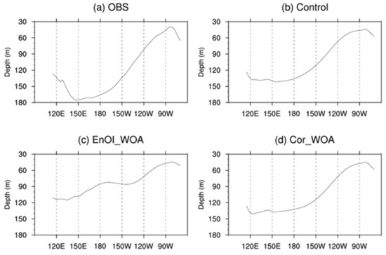
Figure 1.
Long-term average depth of the tropical Pacific thermocline (units: m). (a–d) represent OBS, Control, EnOI_WOA, and Cor_WOA.
As mentioned earlier, the ocean current plays a role in the model simulation, and the SSH has good correspondence with the ocean current, allowing it to largely represent the thermal and dynamic changes in the whole upper layer of the ocean [68]. In the results of the two schemes, there are also some differences between the SSH and current field.
As shown in Figure 2, the OBS mainly shows an obvious westward current influenced by the tropical trade wind, with a relatively small SSH in the east. These similar characteristics are reflected in the results of the Control but with a stronger westward flow than OBS in the whole tropical Pacific. The Cor_WOA has consistent features with the Control, but in the EnOI_WOA, there is no obvious coordination with the Control or OBS in the tropical western Pacific and eastern Indian Ocean, which the eastward countercurrent (−5–5° N, 160–190° E and 0°, 70–90° E) does not correspond to the position of the observed north equatorial countercurrent (5–10° N, 130–155° E and −5° N, 45–65° E). The SSH distribution (the three groups of model tests have similar geoids, so their spatial mean values are directly shown here, rather than the anomaly values of removing the mean values) simulated by the model is basically similar to the OBS distribution features. The SSH values in some regions are not in agreement between the OBS and the model results; they are mainly due to the bias of the model. The large value areas are located in the western Pacific and central Indian Ocean, while in the eastern tropical Pacific, the SSH is relatively small. The SSH of EnOI_WOA in the tropical western Pacific is lower than the Control and Cor_WOA. The current field and SSH are different in the tropical western Pacific, where the thermocline also shows a difference between the two correction schemes. Therefore, we can reasonably assume that the reason for this difference is the current field and sea temperature being inconsistent under EnOI_WOA.
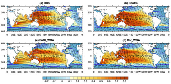
Figure 2.
Long-term average horizontal distribution of the global sea surface height (shaded, unit: m) and current field (arrow, unit: m/s). (a–d) represent OBS, Control, EnOI_WOA, and Cor_WOA.
To evaluate this inconsistency, we selected the tropical western Pacific with the most significant differences for further presentation and analysis. As shown in Figure 3, the results of the Control and Cor_WOA showed similar characteristics for the SSH and horizontal current. The horizontal current is uniformly oriented westward in the tropical western Pacific, but the Cor_WOA indicates a low-value area of SSH around 10° S in the western Pacific. In the results of EnOI_WOA, there is an eastward current near the equator, which is diametrically opposite to the results of the Control and Cor_WOA. There are significant inconsistencies in the distribution and intensity between the eastward countercurrent in EnOI_WOA and OBS. According to the description of the two correction schemes in Section 2.3 and Section 2.4, the setup of model error Rm and observation error Ro are identical. Therefore, the sea temperature obtained by them in their correction step should be the same. Consequently, the adjustment of the sea temperature bias in EnOI_WOA may produce inconsistent adjustments to the current field in data assimilation. In the next section, we seek to uncover the cause of this mismatched countercurrent and determine whether it is affected by the weakening of trade winds or the influence of the ocean’s own multi-variable adjustment.
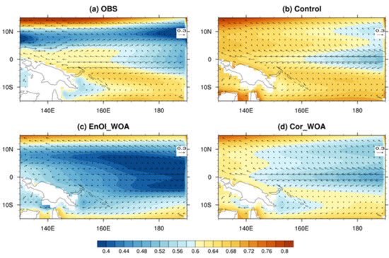
Figure 3.
Long-term average horizontal distribution of the sea surface height (shaded, unit: m) and current field (arrow, unit: m/s) in the tropical western Pacific. (a–d) represent OBS, Control, EnOI_WOA, and Cor_WOA.
3.2. Analysis of the Causes of the Inconsistent Current Field
In the previous section, there were obvious differences between the results of the two correction schemes in the tropical Pacific. In the following section, we seek to explain these differences, especially the inconsistent adjustment of the current field and the reason why this inconsistency affected the correction process through the multi-variable adjustment in the EnOI.
The air–sea interactions cannot be ignored in the coupled model, so we first consider whether the inconsistent current field is affected by atmospheric variables such as the wind. As shown in Figure 4, the three test results of the model simulation are basically consistent with the observed distribution. There are no obvious differences in the distribution of the high- or low-pressure centers and horizontal wind. In the inconsistent areas (i.e., the western tropical Pacific and the eastern Indian Ocean), the southeast and northeast trade winds are still dominant. In the EnOI_WOA, the results of the trade winds slightly weakened, which is consistent with the range of uplift thermocline in the tropical western Pacific. However, the original wind direction does not change here. This indicates that wind weakening is not the main reason for the above inconsistent current field but may still have a slight impact on the horizontal current field.
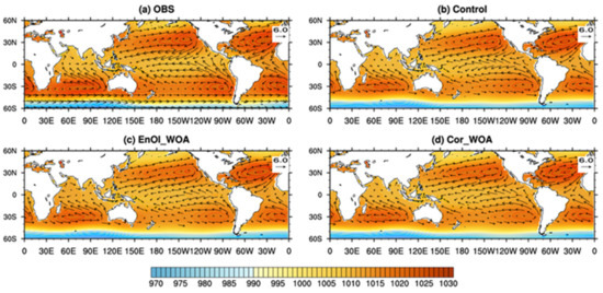
Figure 4.
Long-term mean distribution of the global sea level pressure (unit: hPa) and surface wind (unit: m/s). (a–d) represent OBS, Control, EnOI_WOA, and Cor_WOA.
If the weakened trade winds are not the main result of an inconsistent adjustment of the current field, it is possible that multi-variable adjustment in the ocean leads to the occurrence of a mismatched countercurrent. As shown in Figure 5, the temperature in the upper 400 m of the sea maintains a similar relationship between the Cor_WOA and Control. Both values show a high positive correlation with the surface, which quickly changes to 0 around 100 m and then maintains a high negative correlation after gradually deepening. OBS also shows similar characteristics. However, the results below 100 m show no negative correlation but remain largely around 0. The EnOI_WOA, on the other hand, is obviously different from the other tests. With the maximum positive correlation, the EnOI_WOA value decays rapidly to about 0.4 at a depth of around 100 m. With an increase in depth, the correlation coefficient no longer changes significantly. Compared with the negative correlation of other results below 100 m, the correlation coefficient remains around 0.4. That is to say, the change of sea temperature recorded in EnOI_WOA is obviously different from that in other tests (the correlation in WOA data is similar to the Cor_WOA, but quite different with the EnOI_WOA).
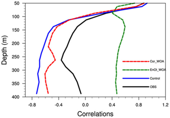
Figure 5.
The correlation between SST and the upper 400 m sea temperature in the western tropical Pacific: black solid line, OBS; blue solid line, Control; green dashed line, EnOI_WOA; red dashed line, Cor_WOA.
The change in the correlation between the temperature on the surface and upper layers of the sea could be the cause of the bias increase in EnOI_WOA. The cause of this change is likely related to other variables adjusted during assimilation, especially the inconsistent horizontal current field mentioned above. As seen in Figure 6, the Cor_WOA and Control maintain the same relationship in the upper layers, which is basically 0.6 in the upper 100 m, then rapid attenuation at 100–200 m, rapid decrease by −0.6 below 200 m, and then there are no significant changes. However, the OBS rarely shows a correlation between SST and the horizontal current field, with a correlation of only 0.2 at the surface layer and a correlation of 0–0.1 between other depths. The correlation with EnOI_WOA is similar to the correlation between SST and the upper 400 m sea temperature. The attenuation of the correlation coefficient is obvious on the surface layer and is weakened and maintained between −0.2 and −0.3 after reaching 100 m, showing completely different characteristics from the other tests.
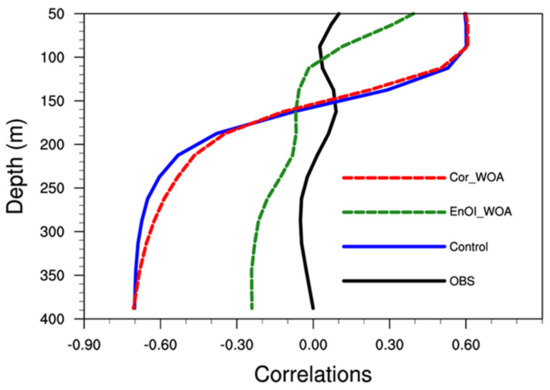
Figure 6.
The correlation between SST and the upper 400 m horizontal current in the western tropical Pacific: black solid line, OBS; blue solid line, Control; green dashed line, EnOI_WOA; red dashed line, Cor_WOA.
In our EnOI approach, the vertical current is not adjusted during assimilation; instead, it changes in the next step of model integration after assimilation. Therefore, the differences between the results of the vertical current in the three model simulation tests are not obvious (Figure 7b–d), which basically reflects the characteristics of a strong downward current in the eastern Pacific and a weak current in the western Pacific. The OBS is almost opposite the model results, showing obvious upwelling in the east and the main subsidence area in the west. This indicates that the vertical current may be the reason why the correlations between the current field and sea temperature in the model results are different with OBS but not why inconsistent adjustment occurs after assimilation.
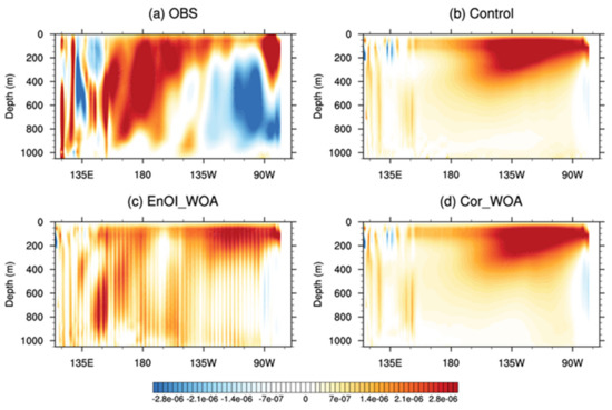
Figure 7.
Long-term mean vertical profile of the vertical current in the tropical Pacific (unit, m/s): (a) OBS; (b) Control; (c) EnOI_WOA; (d) Cor_WOA.
There is a certain bias in the model’s current field that causes the unreasonable correlations between temperature and ocean current in the background matrix (the correlations between SST and the subsurface fields of temperature and current in the background matrix correspond to the correlations in the Control). This kind of unreasonable relationship is introduced into the assimilation through the background matrix, which causes current–field incongruity when assimilating sea temperature data, resulting in inconsistent adjustments. Our new bias correction scheme can adjust the sea temperature without introducing too much information or adjusting other variables during correction. From the results, we can see that this method can successfully solve the inconsistent problem of the current field.
According to the previous results, the inconsistency is most likely caused by an adjustment of the ocean interior. Therefore, we carried out a heat budget analysis on the tropical Pacific. The content discussed in this paper is the long-term mean state, so we only carried out a simple analysis of the climate mean state. To avoid the boundary problem, we chose the whole tropical Pacific for calculations, and Figure 8 illustrates the results of the inconsistent region. Among the four item results, Q is the largest, but the differences between the four tests are not obvious, indicating that Q is not the cause of the difference. The proportions of the other items are generally equal, but the proportion of EnOI_WOA is significantly larger than that of the other tests in Figure 8c. The item w*dT/dz is related to the increase in the vertical current and the cooling of the sea temperature in this area. This item only represents a numerical increase in EnOI_WOA. Indeed, compared to the two items influenced by the horizontal current field, this item is still not the main factor. As shown in Figure 8a,b, the results of the horizontal current field in EnOI_WOA directly change the sign, which is contrary to the other tests (especially the change in the u direction). This may indicate that the horizontal current field is the main cause of the inconsistency.
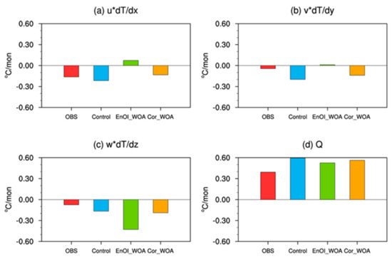
Figure 8.
The average of the heat budget in the western tropical Pacific (−5–5° N, 160–190° E): (a) u*dT/dx; (b) v*dT/dy; (c) w*dT/dz; (d) Q; red, OBS; blue, Control; green, EnOI_WOA; orange, Cor_WOA.
Since the first term in Figure 8a means that the impaction term of the u-directional current field could be the main factor, this term should be given further spatial distribution over the whole tropical Pacific. The EnOI_WOA (Figure 9c) presents exactly the opposite effect to the other tests in the almost equatorial Pacific. In the other tests, this item involves obtaining heat in the ocean (the symbols represent the opposite meaning), while this item in EnOI_WOA involves releasing heat in this area. Due to the inconsistent adjustment of the current field, the heat originally stored in the western Pacific is lost, leading to a decrease in sea temperature. This decrease in sea temperature, in turn, will produce an incorrect direction and change the horizontal current field under EnOI_WOA, thus further aggravating this inconsistency.
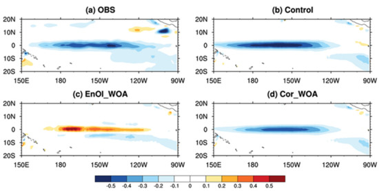
Figure 9.
Spatial distribution of u*dT/dx in the tropical Pacific: (a) OBS; (b) Control; (c) EnOI_WOA; (d) Cor_WOA.
To better describe the heat transfer in the upper layer of the ocean, we selected two areas with the same grid range on the eastern and western sides of the tropical Pacific and calculated the regional average of the sea temperature (Figure 10). After subtracting the east side from the west side, the sea temperature difference at a depth of 50–200 m was shown to be the most significant, while the sea temperature difference of the EnOI_WOA was more than 3 centigrade. This result is similar to the tropical thermocline shown in Figure 1c, corresponding to its shallowness. This means that the heat is not stored in the west but transferred to the east under the influence of the inconsistent current field, thereby warming the sea temperature in the east and reducing the sea temperature difference. Moreover, the difference in sea temperature below 200 m is close to −3 centigrade in the EnOI_WOA; that is, the sea temperature in the west is 3 centigrade lower than that in the east, meaning that under the influence of the current field, the heat was not stored after it was transferred down into the deeper ocean in the west. The new bias correction scheme results maintain good consistency with the observations in the above analysis, indicating that this scheme can not only overcome the aforementioned inconsistency but also improve the simulation results of the model.
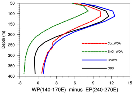
Figure 10.
The vertical profile of the difference in sea temperature between the tropical western Pacific (−5–5° N, 140–170° E) and the eastern Pacific (−5–5° N, 240–270° E) (unit, °C): black solid, OBS; blue solid, Control; green dashed, EnOI_WOA; red dashed, Cor_WOA.
4. Discussion
The explanation for the current field inconsistent adjustments in this paper is still relatively preliminary and is only concerned with the heat transfer introduced by the assimilated sea temperature. A coupled model that involves significant dynamic and thermal conversion mechanisms is worthy of further discussion and analysis. For example, the influence of equatorial subsurface current and the important role of salinity in ocean change should be considered. In the future, correcting the salinity or other variables through different data should be considered to test the relevant changes and reveal the physical mechanisms.
Because the new ensemble-based bias correction scheme does not produce incoordination in CAS-ESM-C, we thought there should be no adjustment needed for other variables except for sea temperature during corrections. Whether there are similar results in other coupled models, it is still necessary to carry out corresponding tests. Accordingly, whether the EnOI method, which is widely used in data assimilation of the coupled model, has a similar problem to that mentioned in this paper during multi-variable assimilation, it also needs more model results to test. In the new version of the CAS-ESM-C, the simulation of each sub-model and the flux exchange between them are improved. Based on the idea of ensemble forecast, we further superimposed the model disturbance with the sea temperature climate state observation data to correct the model bias more reasonably, such as in high-resolution regional ocean models without coupled atmospheric models, such as ROMs and HYCOM. Using coarse resolution sea temperature climate state observation data, whether this correction scheme could produce reasonable and effective results also needs to be further tested.
5. Conclusions
In this study, we used WOA13 sea temperature climate data based on the EnOI approach and ensemble idea to design two bias correction schemes of sea temperature bias in the coupled model (CAS-ESM-C) and compare the results of these two schemes. The ensemble-based bias correction scheme could effectively avoid the inconsistent adjustments, and the model simulation bias increased, which are in EnOI scheme:
(1) The main manifestation of inconsistency is in the tropical western Pacific and the eastern Indian Ocean. According to the correlation analysis of SST with upper sea temperature and horizontal current field, we have determined that the main reason for increased bias is the influence of the current field’s inconsistent adjustment.
(2) The ensemble-based bias correction scheme could effectively overcome the inconsistent adjustment though only correcting the sea temperature at the correction step. The vertical velocity not involved in the EnOI approach has not changed significantly, meaning that vertical current is not the main factor causing this inconsistency; on the other hand, it also suggests that other variables in the ocean model that are not directly adjusted in the correction are almost unaffected. Therefore, the ensemble-based bias correction scheme could reduce the original model sea temperature bias and achieved a reasonable model simulation.
(3) The atmospheric model is not significant for the formation of this inconsistency, mainly due to the adjustment of the ocean model. Due to the negative bias of the model sea temperature in the tropic Pacific, a quantity of heat would be introduced into the upper ocean when assimilated sea temperature. The wind–evaporation feedback in the atmospheric model consumed part of this heat, but from our results, its influences on this heat should be small. In the ocean model, the vertical velocity is smaller on the tropical western Pacific, which is not conducive to the downward heat transfer and storage. Under the influence of the horizontal current field, the heat is mainly transferred to the east, weakening the trade wind through the air–sea interaction process, further strengthening the current field to east, and transferring more heat, which eventually leads to the increased bias of sea temperature simulation.
Author Contributions
Conceptualization, F.Z. and J.Z.; methodology, M.D. and F.Z.; validation, M.D., F.Z. and R.L.; formal analysis, M.D. and R.L.; investigation, M.D. and K.Y.; resources, F.Z. and J.Z.; data curation, M.D., F.Z. and K.Y.; writing—original draft preparation, M.D.; writing—review and editing, R.L. and K.Y.; supervision, F.Z. and J.Z.; project administration, F.Z.; funding acquisition, F.Z. All authors have read and agreed to the published version of the manuscript.
Funding
This research was funded by the Key Research Program of Frontier Sciences, CAS (Grant No. ZDBS-LY-DQC010), the National Natural Science Foundation of China (Grant No. 41876012; 41861144015), and the Strategic Priority Research Program of the Chinese Academy of Sciences (Grant No. XDB42000000).
Institutional Review Board Statement
Not applicable.
Informed Consent Statement
Not applicable.
Data Availability Statement
The data WOA13 V2 (https://www.nodc.noaa.gov/cgi-bin/OC5/woa13/woa13.pl?parameter=t), GODAS (https://www.godae-oceanview.org/outreach/meetings-workshops/task-team-meetings/godae-oceanview-gsop-clivar-workshop/presentations/), and ERA-interim (https://www.ecmwf.int/en/forecasts/datasets/reanalysis-datasets/era-interim) are available in public repositories. The two correction schemes outputs for this paper are also available in public repositories (https://figshare.com/s/af256fa51304ff473ba1), accessed on 28 June 2021.
Acknowledgments
The work was carried out at the National Supercomputer Center in Tianjin, and the calculations were performed on TianHe-1(A).
Conflicts of Interest
The authors declare no conflict of interest.
References
- Flato, G.; Marotzke, J.; Abiodun, B.; Braconnot, P.; Chou, S.C.; Collins, W.; Cox, P.; Driouech, F.; Emori, S.; Eyring, V. Evaluation of climate models. In Climate Change 2013: The Physical Science Basis. Contribution of Working Group I to the Fifth Assessment Report of the Intergovernmental Panel on Climate Change; Solomon, S., Qin, D., Manning, M., Chen, Z., Marq, M., Eds.; Cambridge University Press: Cambridge, UK, 2014; pp. 741–866. [Google Scholar]
- Karl, T.R.; Trenberth, K.E. Modern global climate change. Science 2003, 302, 1719–1723. [Google Scholar] [CrossRef]
- Behringer, D.W.; Ji, M.; Leetmaa, A. An improved coupled model for ENSO prediction and implications for ocean initialization. Part I: The Ocean Data Assimilation System. Mon. Weather Rev. 1998, 126, 1013–1021. [Google Scholar] [CrossRef]
- Brune, S.; Nerger, L.; Baehr, J. Assimilation of oceanic observations in a global coupled Earth system model with the SEIK filter. Ocean Model. 2015, 96, 254–264. [Google Scholar] [CrossRef]
- Fujii, Y.; Nakaegawa, T.; Matsumoto, S.; Yasuda, T.; Yamanaka, G.; Kamachi, M. Coupled climate simulation by constraining ocean fields in a coupled model with ocean data. J. Clim. 2009, 22, 5541–5557. [Google Scholar] [CrossRef]
- Oke, P.R.; Brassington, G.B.; Griffin, D.A.; Schiller, A. The Bluelink ocean data assimilation system (BODAS). Ocean Model. 2008, 21, 46–70. [Google Scholar] [CrossRef]
- Xie, J.P.; Zhu, J.; Xu, L.; Guo, P.W. Evaluation of mid-depth currents of NCEP reanalysis data in the tropical Pacific using ARGO float position information. Adv. Atmos. Sci. 2005, 22, 677–684. [Google Scholar]
- Xue, Y.; Wen, C.; Yang, X.; Behringer, D.; Kumar, A.; Vecchi, G.; Rosati, A.; Gudgel, R. Evaluation of tropical Pacific observing systems using NCEP and GFDL ocean data assimilation systems. Clim. Dyn. 2017, 49, 843–868. [Google Scholar] [CrossRef]
- Karspeck, A.R.; Yeager, S.; Danabasoglu, G.; Hoar, T.; Tribbia, J. An ensemble adjustment Kalman Filter for the CCSM4 ocean component. J. Clim. 2013, 26, 7392–7413. [Google Scholar] [CrossRef]
- Dai, A. Precipitation characteristics in eighteen coupled climate models. J. Clim. 2006, 19, 4605–4630. [Google Scholar] [CrossRef]
- Tian, B.J. Spread of model climate sensitivity linked to double-Intertropical Convergence Zone bias. Geophys. Res. Lett. 2015, 42, 4133–4141. [Google Scholar] [CrossRef]
- Lin, J.L. The double-ITCZ problem in IPCC AR4 coupled GCMs: Ocean-atmosphere feedback analysis. J. Clim. 2007, 20, 4497–4525. [Google Scholar] [CrossRef]
- Kug, J.-S.; Ham, Y.-G.; Lee, J.-Y.; Jin, F.-F. Improved simulation of two types of El Niño in CMIP5 models. Environ. Res. Lett. 2012, 7, 034002. [Google Scholar] [CrossRef]
- Latif, M.; Sperber, K.; Arblaster, J.; Braconnot, P.; Chen, D.; Colman, A.; Cubasch, U.; Cooper, C.; Delecluse, P.; DeWitt, D.; et al. ENSIP: The El Nino simulation intercomparison project. Clim. Dyn. 2001, 18, 255–276. [Google Scholar] [CrossRef]
- Delworth, T.L.; Broccoli, A.J.; Rosati, A.; Stouffer, R.J.; Balaji, V.; Beesley, J.A.; Cooke, W.F.; Dixon, K.W.; Dunne, J.; Dunne, K.A.; et al. GFDL’s CM2 global coupled climate models. Part I: Formulation and simulation characteristics. J. Clim. 2006, 19, 643–674. [Google Scholar] [CrossRef]
- Gainusa-Bogdan, A.; Hourdin, F.; Traore, A.K.; Braconnot, P. Omens of coupled model biases in the CMIP5 AMIP simulations. Clim. Dyn. 2018, 51, 2927–2941. [Google Scholar] [CrossRef]
- Meehl, G.A.; Covey, C.; McAvaney, B.; Latif, M.; Stouffer, R.J. Overview of the coupled model intercomparison project. Bull. Am. Meteorol. Soc. 2005, 86, 89–93. [Google Scholar] [CrossRef]
- Zhang, S.; Rosati, A. An inflated ensemble filter for ocean data assimilation with a biased coupled GCM. Mon. Weather Rev. 2010, 138, 3905–3931. [Google Scholar] [CrossRef]
- Zhang, S.; Chang, Y.S.; Yang, X.; Rosati, A. Balanced and coherent climate estimation by combining data with a biased coupled model. J. Clim. 2014, 27, 1302–1314. [Google Scholar] [CrossRef]
- Zhang, X.; Zhang, S.; Liu, Z.; Wu, X.; Han, G. Correction of biased climate simulated by biased physics through parameter estimation in an intermediate coupled model. Clim. Dyn. 2016, 47, 1899–1912. [Google Scholar] [CrossRef]
- Chen, D.; Cane, C.M.; Zebiak, S.E.; Canizares, R.; Kaplan, A. Bias correction of an ocean-atmosphere coupled model. Geophys. Res. Lett. 2000, 27, 2585–2588. [Google Scholar] [CrossRef]
- Chang, Y.-S.; Zhang, S.; Rosati, A.; Delworth, T.L.; Stern, W.F. An assessment of oceanic variability for 1960–2010 from the GFDL ensemble coupled data assimilation. Clim. Dyn. 2013, 40, 775–803. [Google Scholar] [CrossRef]
- Han, G.J.; Zhang, X.F.; Zhang, S.; Wu, X.R.; Liu, Z. Mitigation of coupled model biases induced by dynamical core misfitting through parameter optimization: Simulation with a simple pycnocline prediction model. Nonlinear Process. Geophys. 2014, 21, 357–366. [Google Scholar] [CrossRef]
- Lu, F.; Liu, Z.; Zhang, S.; Jacob, R. Assessing extratropical impact on the tropical bias in coupled climate model with regional coupled data assimilation. Geophys. Res. Lett. 2017, 44, 3384–3392. [Google Scholar] [CrossRef]
- Dawson, A.; Matthews, A.J.; Stevens, D.P.; Roberts, M.J.; Vidale, P.L. Importance of oceanic resolution and mean state on the extra-tropical response to El Nio in a matrix of coupled models. Clim. Dyn. 2013, 41, 1439–1452. [Google Scholar] [CrossRef]
- Fang, X.H.; Zheng, F.; Zhu, J. The cloud-radiative effect when simulating strength asymmetry in two types of El Nino events using CMIP5 models. J. Geophys. Res. Ocean. 2015, 120, 4357–4369. [Google Scholar] [CrossRef]
- Zheng, F.; Zhu, J. Improved ensemble-mean forecasting of ENSO events by a zero-mean stochastic error model of an intermediate coupled model. Clim. Dyn. 2016, 47, 3901–3915. [Google Scholar] [CrossRef]
- Zheng, F.; Zhang, R.H. Interannually varying salinity effects on ENSO in the tropical pacific: A diagnostic analysis from Argo. Ocean Dyn. 2015, 65, 691–705. [Google Scholar] [CrossRef]
- Zheng, F.; Yu, J.-Y. Contrasting the skills and biases of deterministic predictions for the two types of El Nino. Adv. Atmos. Sci. 2017, 34, 1395–1403. [Google Scholar] [CrossRef]
- Cooper, M.; Haines, K. Altimetric assimilation with water property conservation. J. Geophys. Res. Ocean. 1996, 101, 1059–1077. [Google Scholar] [CrossRef]
- Fujii, Y.; Matsumoto, S.; Kamachi, M.; Ishizaki, S. Estimation of the Equatorial Pacific Salinity Field Using Ocean Data Assimilation Systems. Adv. Geosci. 2010, 18, 197–212. [Google Scholar] [CrossRef]
- Zhang, S.; Liu, Z.; Zhang, X.; Wu, X.; Han, G.; Zhao, Y.; Yu, X.; Liu, C.; Liu, Y.; Wu, S.; et al. Coupled data assimilation and parameter estimation in coupled ocean-atmosphere models: A review. Clim. Dyn. 2020, 54, 5127–5144. [Google Scholar] [CrossRef]
- Yan, C.X.; Zhu, J.; Li, R.F.; Zhou, G.Q. Roles of vertical correlations of background error and T-S relations in estimation of temperature and salinity profiles from sea surface dynamic height. J. Geophys. Res. Ocean. 2004, 109. [Google Scholar] [CrossRef]
- Derber, J.; Bouttier, F. A reformulation of the background error covariance in the ECMWF global data assimilation system. Tellus A Dyn. Meteorol. Oceanogr. 1999, 51, 195–221. [Google Scholar] [CrossRef]
- Ji, M.; Leetmaa, A.; Derber, J. An ocean analysis system for seasonal to interannual climate studies. Mon. Weather Rev. 1995, 123, 460–481. [Google Scholar] [CrossRef]
- Kimoto, M.; Yoshikawa, I.; Ishii, M. An ocean data assimilation system for climate monitoring. J. Meteorol. Soc. Jpn. 1997, 75, 471–487. [Google Scholar] [CrossRef]
- Counillon, F.; Keenlyside, N.; Bethke, I.; Wang, Y.; Billeau, S.; Shen, M.L.; Bentsen, M. Flow-dependent assimilation of sea surface temperature in isopycnal coordinates with the Norwegian Climate Prediction Model. Tellus A Dyn. Meteorol. Oceanogr. 2016, 68, 32437. [Google Scholar] [CrossRef]
- Chen, X.R.; Wang, H.; Zheng, F.; Cai, Q. An ensemble-based SST nudging method proposed for correcting the subsurface temperature field in climate model. Acta Oceanol. Sin. 2020, 39, 73–80. [Google Scholar] [CrossRef]
- Carton, J.A.; Giese, B.S.; Cao, X.H.; Miller, L. Impact of altimeter, thermistor, and expendable bathythermograph data on retrospective analyses of the tropical Pacific Ocean. J. Geophys. Res. Ocean. 1996, 101, 14147–14159. [Google Scholar] [CrossRef]
- Luo, H.; Zheng, F.; Zhu, J. Evaluation of oceanic surface observation for reproducing the upper ocean structure in ECHAM5/MPI-OM. J. Geophys. Res. Ocean. 2017, 122, 9695–9711. [Google Scholar] [CrossRef]
- Bjerknes, J. A possible response of atmospheric Hadley circulation to equatorial anomalies of ocean temperature. Tellus 1966, 18, 820–829. [Google Scholar] [CrossRef]
- Bjerknes, J. Atmospheric teleconnections from equatorial pacific. Mon. Weather Rev. 1969, 97, 163–172. [Google Scholar] [CrossRef]
- Gill, A.E. Some simple solutions for heat-induced tropical circulation. Q. J. R. Meteorol. Soc. 1980, 106, 447–462. [Google Scholar] [CrossRef]
- Horel, J.D.; Wallace, J.M. Planetary-scale atmospheric phenomena associated with the southern oscillation. Mon. Weather Rev. 1981, 109, 813–829. [Google Scholar] [CrossRef]
- Jungclaus, J.H.; Keenlyside, N.; Botzet, M.; Haak, H.; Luo, J.J.; Latif, M.; Marotzke, J.; Mikolajewicz, U.; Roeckner, E. Ocean circulation and tropical variability in the coupled model ECHAM5/MPI-OM. J. Clim. 2006, 19, 3952–3972. [Google Scholar] [CrossRef]
- Alexander, M.A.; Blade, I.; Newman, M.; Lanzante, J.R.; Lau, N.C.; Scott, J.D. The atmospheric bridge: The influence of ENSO teleconnections on air-sea interaction over the global oceans. J. Clim. 2002, 15, 2205–2231. [Google Scholar] [CrossRef]
- Jin, F.F. An equatorial ocean recharge paradigm for ENSO. Part I: Conceptual model. J. Atmos. Sci. 1995, 54, 811–829. [Google Scholar] [CrossRef]
- Zheng, F.; Zhu, J.; Zhang, R.-H. Impact of altimetry data on ENSO ensemble initializations and predictions. Geophys. Res. Lett. 2007, 34, L13611. [Google Scholar] [CrossRef]
- Zheng, F.; Fang, X.H.; Zhu, J.; Yu, J.Y.; Li, X.C. Modulation of Bjerknes feedback on the decadal variations in ENSO predictability. Geophys. Res. Lett. 2016, 43, 12560–12568. [Google Scholar] [CrossRef]
- Chen, Y.; Yan, C.; Zhu, J. Assimilation of sea surface temperature in a global hybrid coordinate ocean model. Adv. Atmos. Sci. 2018, 35, 1291–1304. [Google Scholar] [CrossRef]
- Su, T.; Xue, F.; Sun, H.; Zhou, G. The El Nino-Southern Oscillation cycle simulated by the climate system model of Chinese Academy of Sciences. Acta Oceanol. Sin. 2015, 34, 55–65. [Google Scholar] [CrossRef]
- Dong, X.; Su, T.H.; Wang, J.; Lin, R.P. Decadal variation of the Aleutian Low-Icelandic Low seesaw simulated by a climate system model (CAS-ESM-C). Atmos. Ocean. Sci. Lett. 2014, 7, 110–114. [Google Scholar]
- Dong, X.; Lin, R.P.; Zhu, J.; Lu, Z.T. Evaluation of ocean data assimilation in CAS-ESM-C: Constraining the SST field. Adv. Atmos. Sci. 2016, 33, 795–807. [Google Scholar] [CrossRef]
- Du, M.J.; Zheng, F.; Zhu, J.; Lin, R.P.; Yang, H.-P. A new ensemble-based approach to correct the systematic ocean temperature bias of CAS-ESM-C to improve its simulation and data assimilation abilities. J. Geophys. Res. Ocean. 2020, 125. [Google Scholar] [CrossRef]
- Sun, H.; Zhou, G.; Zeng, Q. Assessments of the climate system model (CAS-ESM-C) using IAP AGCM4 as its atmospheric component. Chin. J. Atmos. Sci. 2012, 36, 215–233. [Google Scholar]
- Zhang, H. Development of IAP Atmospheric General Circulation Model Version 4.0 and Its Climate Simulations; Chinese Academy of Sciences: Beijing, China, 2009. [Google Scholar]
- Liu, H.; Zhang, X.; Wei, L.I.; Yongqiang, Y.U.; Rucong, Y.U. An eddy-permitting oceanic general circulation model and its preliminary evaluation. Adv. Atmos. Sci. 2004, 21, 675–690. [Google Scholar]
- Dickinson, R.E.; Oleson, K.W.; Bonan, G.; Hoffman, F.; Thornton, P.; Vertenstein, M.; Yang, Z.-L.; Zeng, X. The Community Land Model and its climate statistics as a component of the Community Climate System Model. J. Clim. 2006, 19, 2302–2324. [Google Scholar] [CrossRef]
- Boyer, T.P.; Antonov, J.I.; Baranova, O.K.; Garcia, H.E.; Johnson, D.R.; Mishonov, A.V.; O’Brien, T.D.; Seidov, D.; Smolyar, I.; Zweng, M.M.; et al. World ocean database 2013. NOAA atlas NESDIS 2013. [Google Scholar] [CrossRef]
- Behringer, D.; Xue, Y. Evaluation of the global ocean data assimilation system at NCEP: The Pacific Ocean. In Proceedings of the Eighth Symposium on Integrated Observing and Assimilation Systems for Atmosphere, Oceans, and Land Surface, NOAA/NWS/NCEP/EMC, Camp Springs, MD, USA, 11–15 January 2004. [Google Scholar]
- Dee, D.P.; Uppala, S.M.; Simmons, A.J.; Berrisford, P.; Poli, P.; Kobayashi, S.; Andrae, U.; Balmaseda, M.A.; Balsamo, G.; Bauer, P.; et al. The ERA-Interim reanalysis: Configuration and performance of the data assimilation system. Q. J. R. Meteorol. Soc. 2011, 137, 553–597. [Google Scholar] [CrossRef]
- Lorenc, A.C. Analysis methods for numerical weather prediction. Q. J. R. Meteorol. Soc. 1986, 112, 1177–1194. [Google Scholar] [CrossRef]
- Cohn, S.E. An introduction to estimation theory. J. Meteorol. Soc. Jpn. 1997, 75, 257–288. [Google Scholar] [CrossRef]
- Evensen, G. Sequential data assimilation with a nonlinear quasi-geostrophic model using Monte-Carlo methods to forecast error statistics. J. Geophys. Res.-Ocean. 1994, 99, 10143–10162. [Google Scholar] [CrossRef]
- Evensen, G. The Ensemble Kalman Filter: Theoretical formulation and practical implementation. Ocean Dyn. 2003, 53, 343–367. [Google Scholar] [CrossRef]
- Fu, W.; Zhu, J.; Yan, C.; Liu, H. Toward a global ocean data assimilation system based on ensemble optimum interpolation: Altimetry data assimilation experiment. Ocean Dyn. 2009, 59, 587–602. [Google Scholar] [CrossRef]
- Yan, C.; Zhu, J.; Xie, J. An ocean data assimilation system in the Indian Ocean and west Pacific Ocean. Adv. Atmos. Sci. 2015, 32, 1460–1472. [Google Scholar] [CrossRef]
- Carnes, M.R.; Mitchell, J.L.; de Witt, P.W. Synthetic temperature profiles derived from Geosat altimetry: Comparison with air-dropped expendable bathythermograph profiles. J. Geophys. Res.Ocean. 1990, 95, 17979–17992. [Google Scholar] [CrossRef]


Publisher’s Note: MDPI stays neutral with regard to jurisdictional claims in published maps and institutional affiliations. |
© 2021 by the authors. Licensee MDPI, Basel, Switzerland. This article is an open access article distributed under the terms and conditions of the Creative Commons Attribution (CC BY) license (https://creativecommons.org/licenses/by/4.0/).