
Atmospheric and Climatic Drivers of Tide Gauge Sea Level Variability along the East and South Coast of South Africa

 , , and
Abstract
:1. Introduction
2. Data and Methods
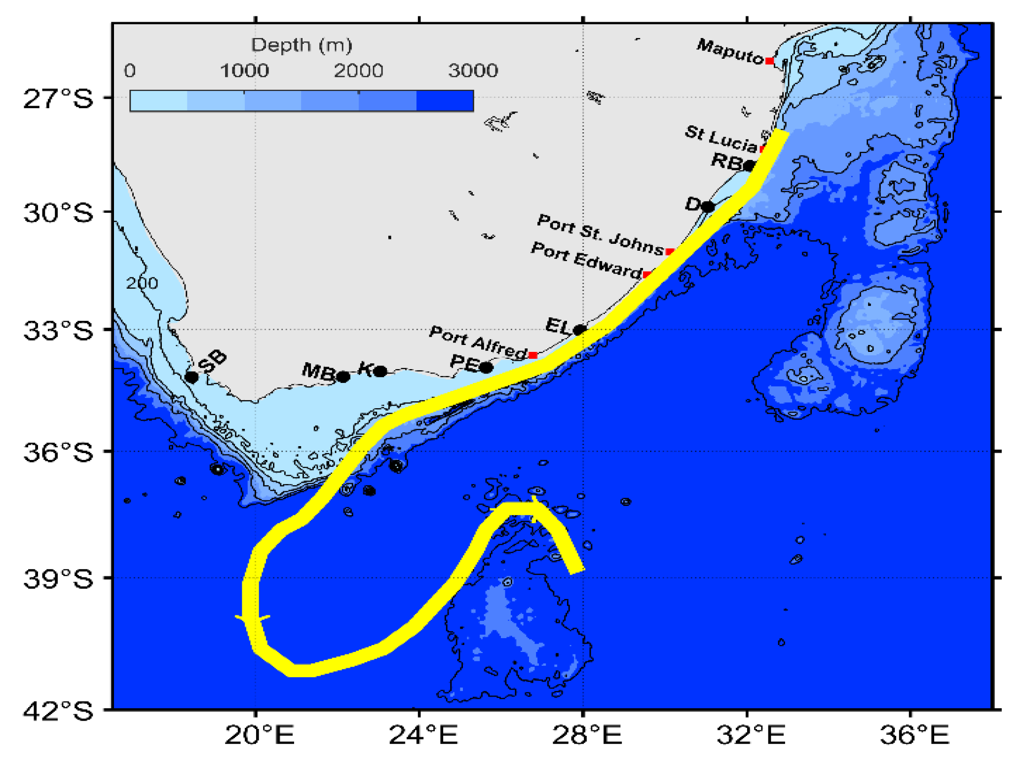
2.1. Data
2.1.1. Sea Level Observations
2.1.2. Large-Scale Oceanographic and Climate Data
Sea Level Pressure
Winds
Extended Reconstructed Sea Surface Temperature
Dipole Mode Index
Multivariate ENSO Index
Southern Annular Mode
2.2. Methods
3. Results
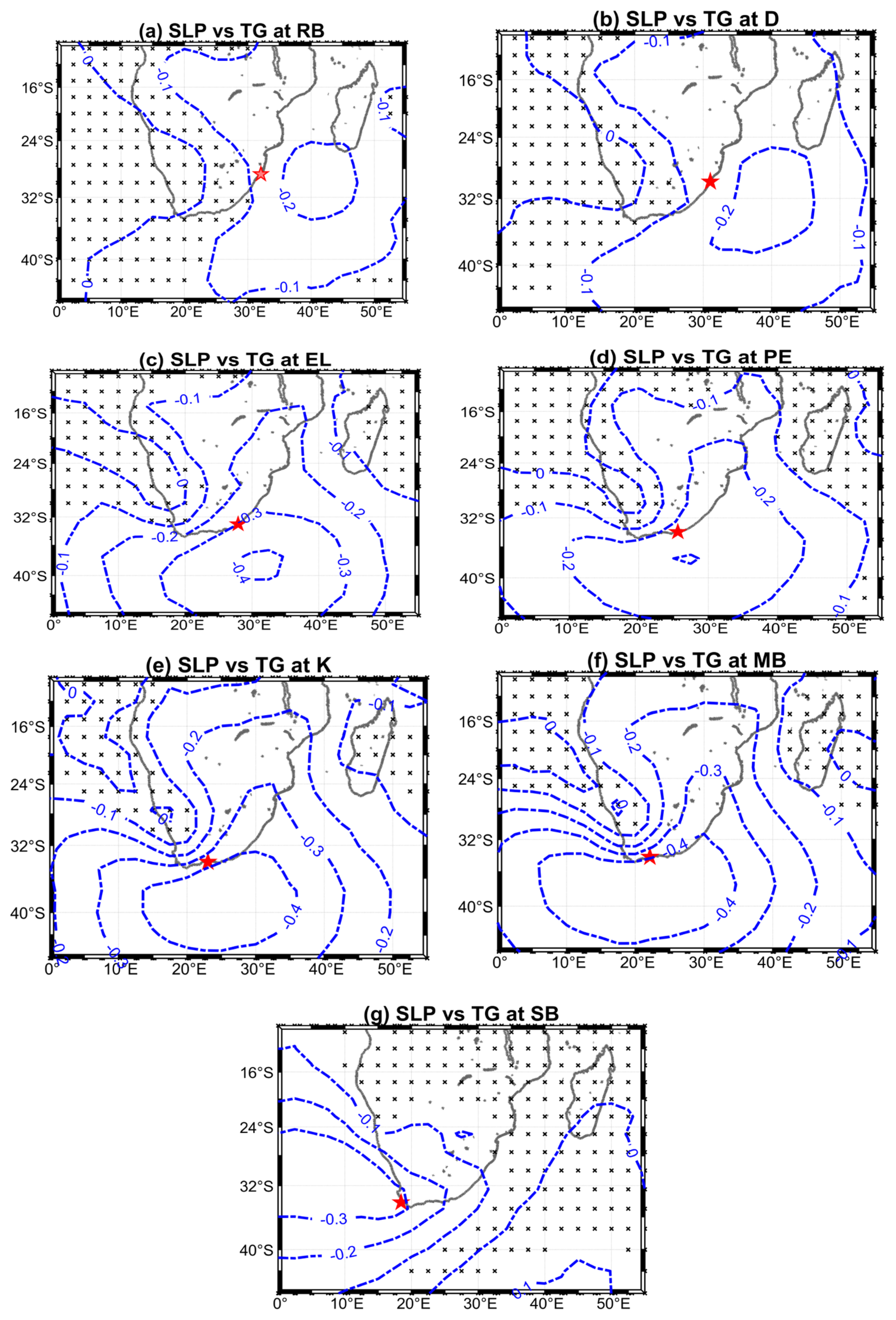
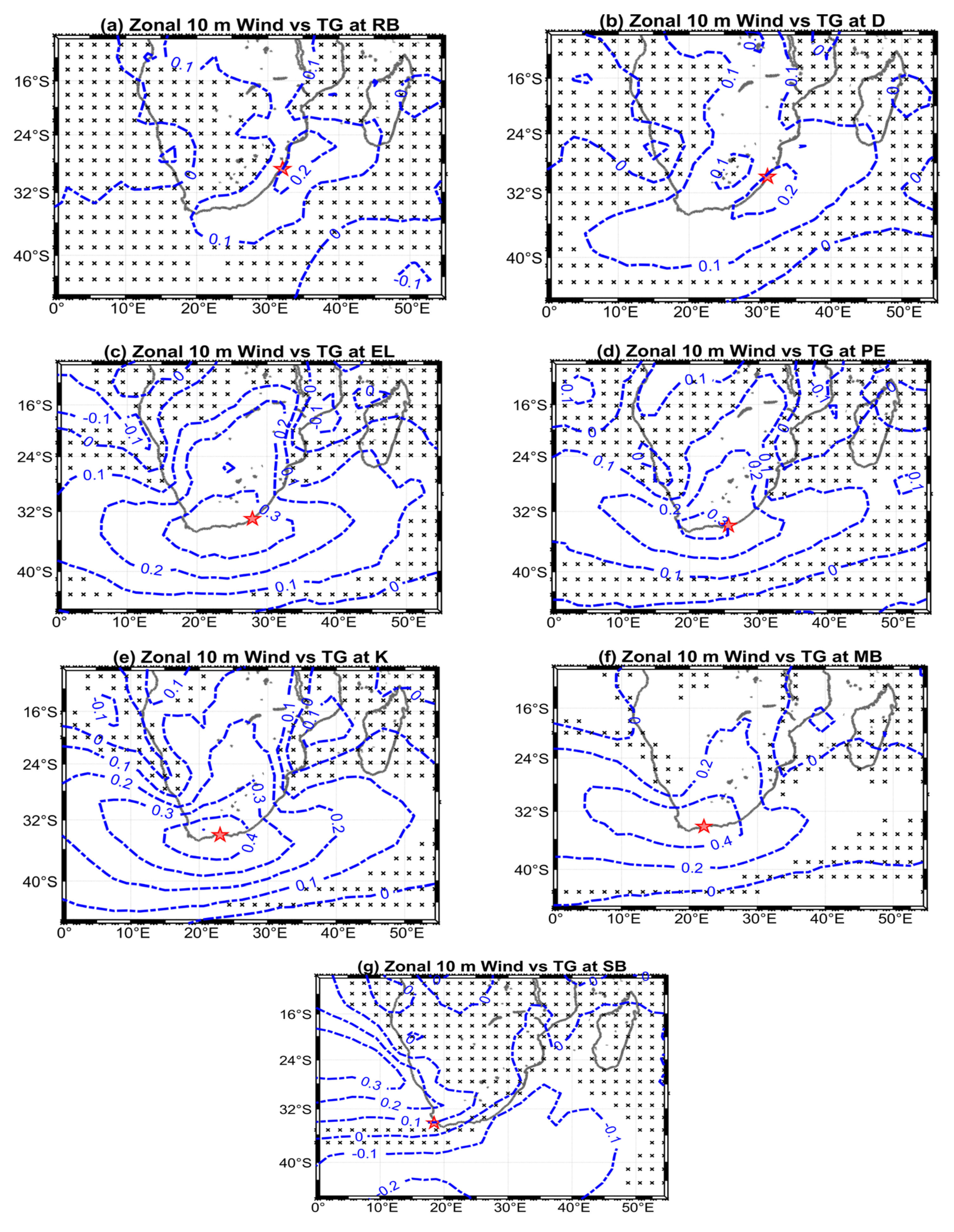
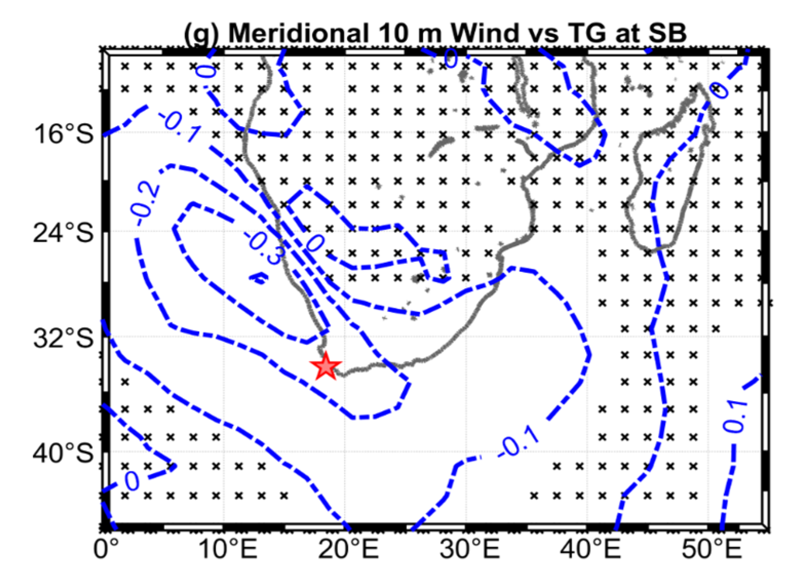
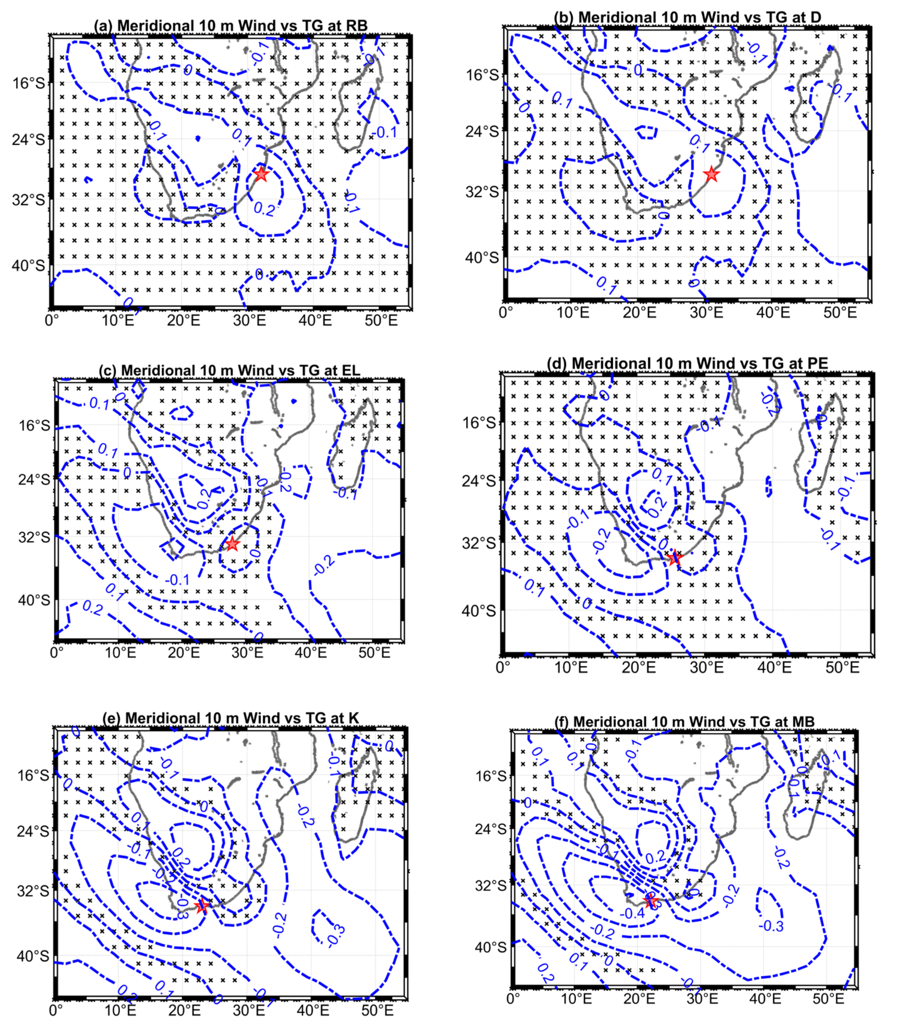
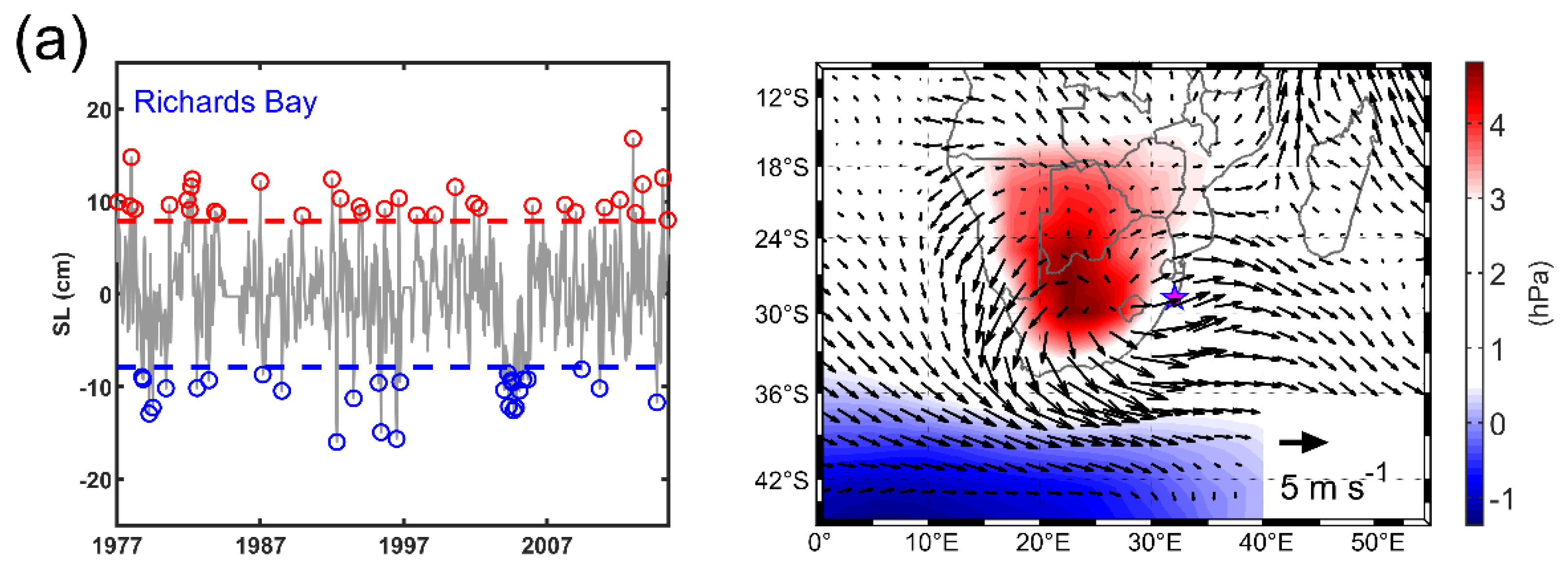
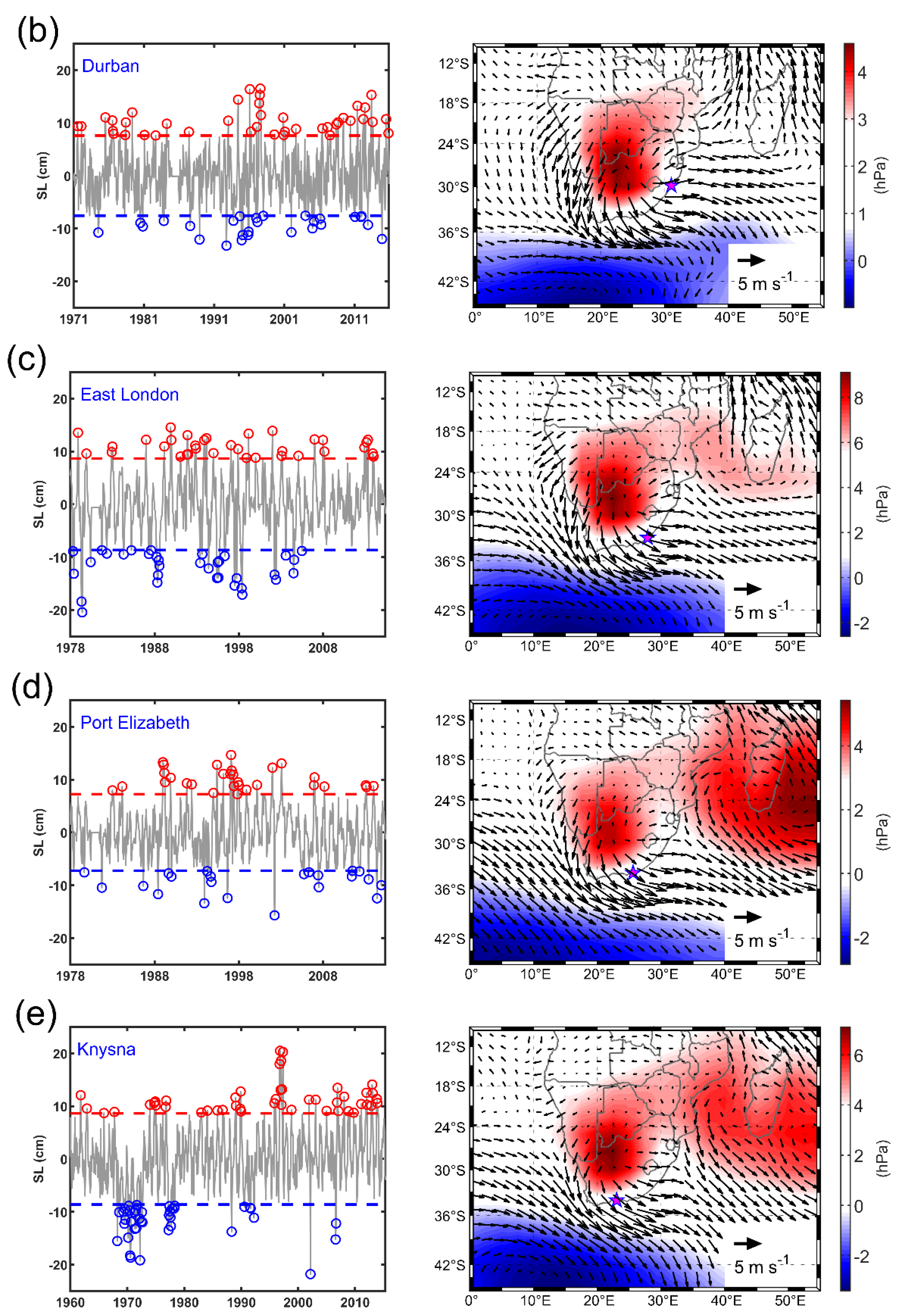
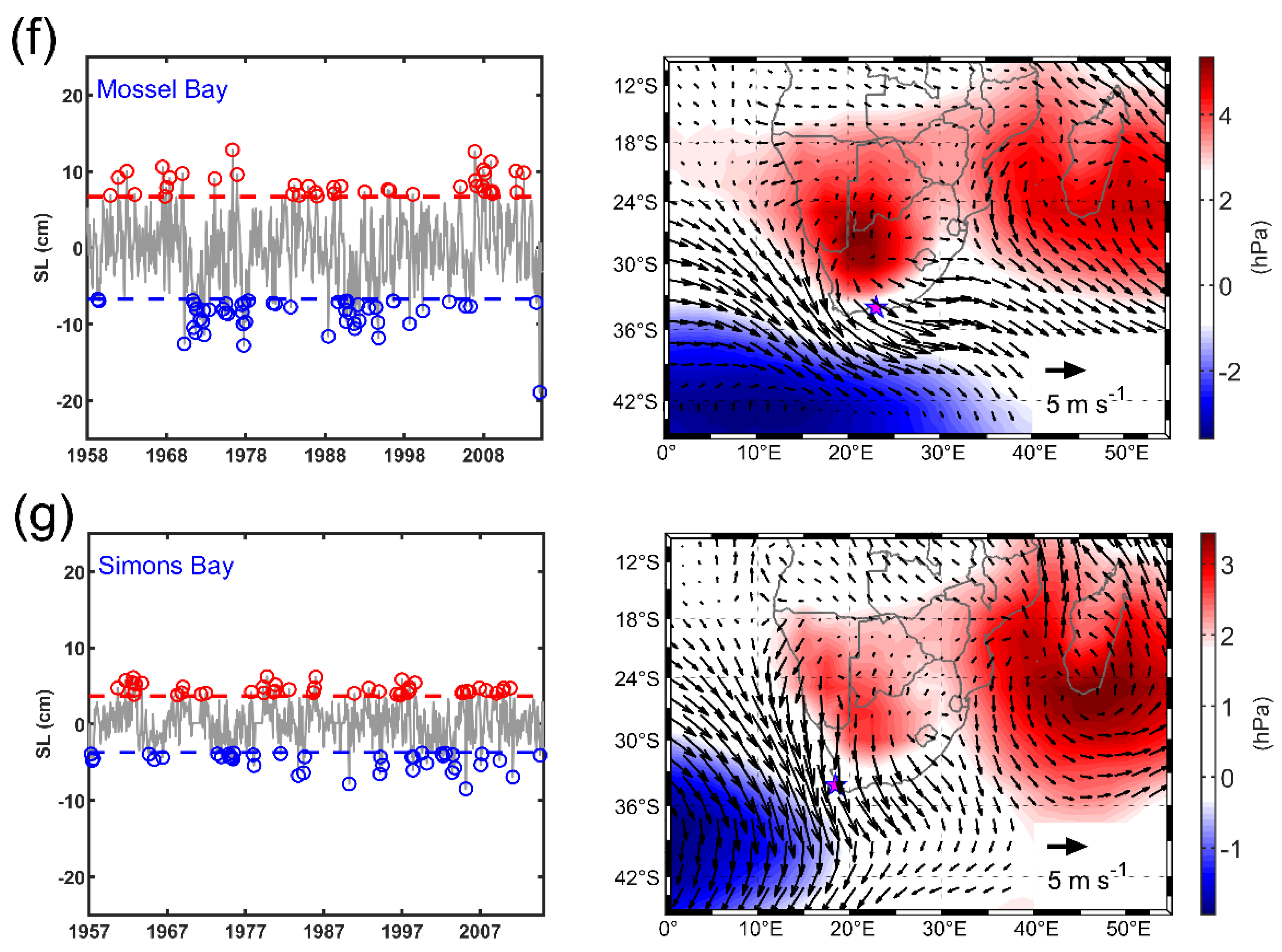
3.1. Drivers of Tide Gauge Sea Level Variability at Sub-Annual Timescales
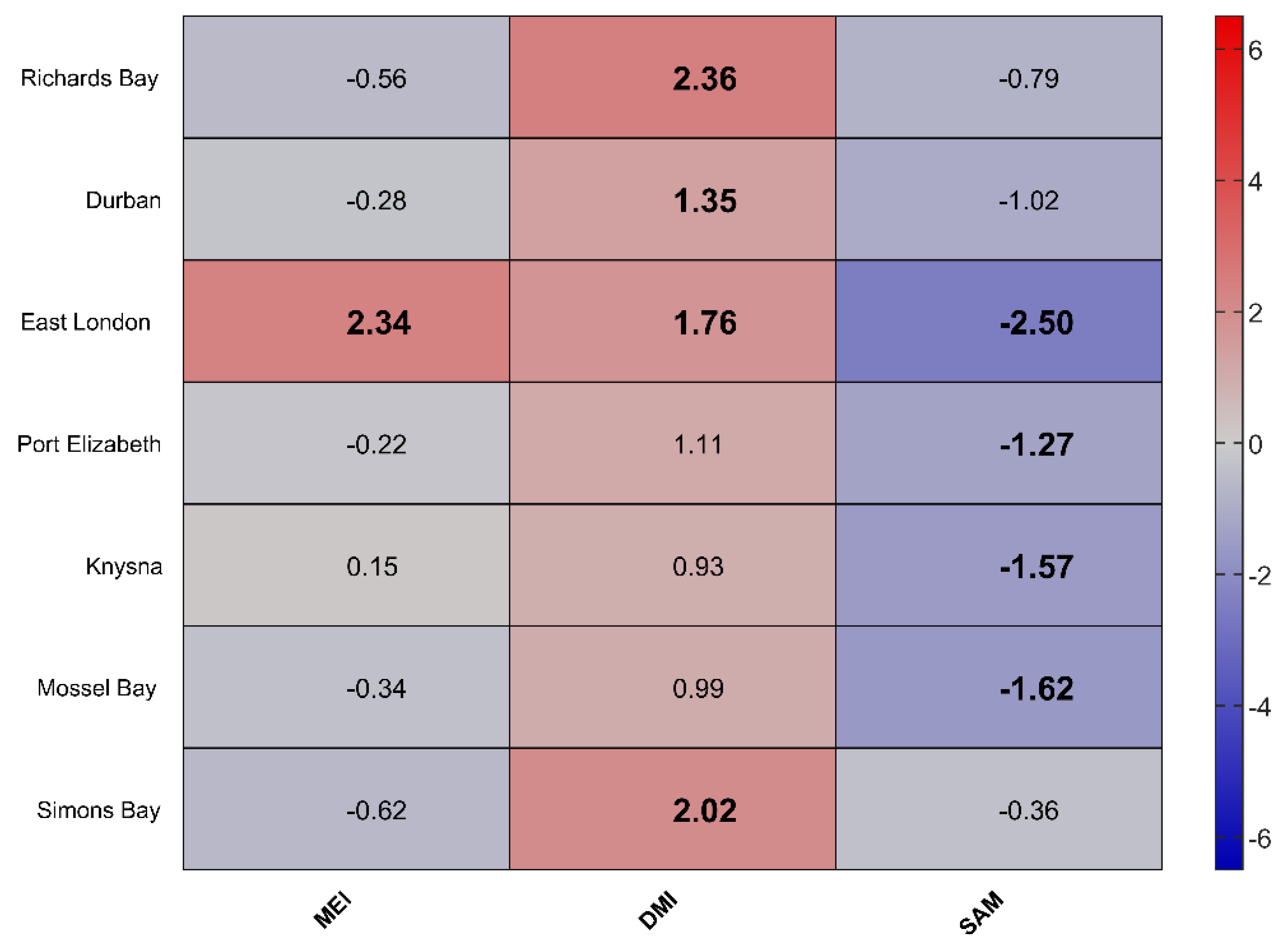
The Response of Coastal Sea Level to Strong Anomalies in the Atmospheric Forcing
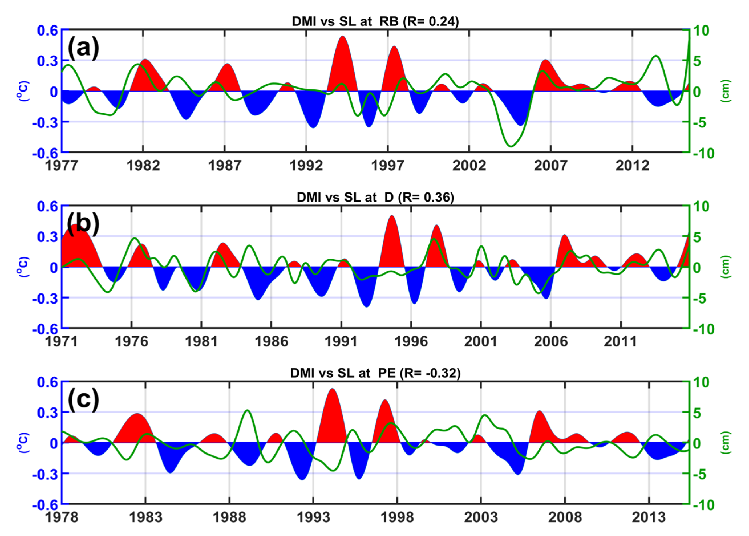
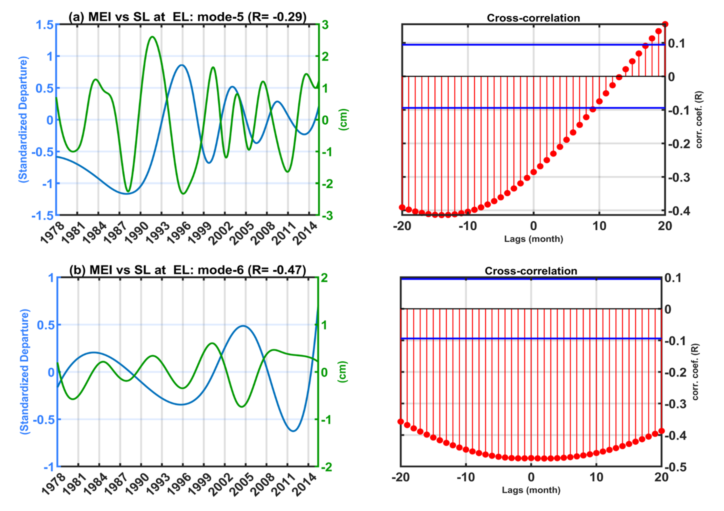
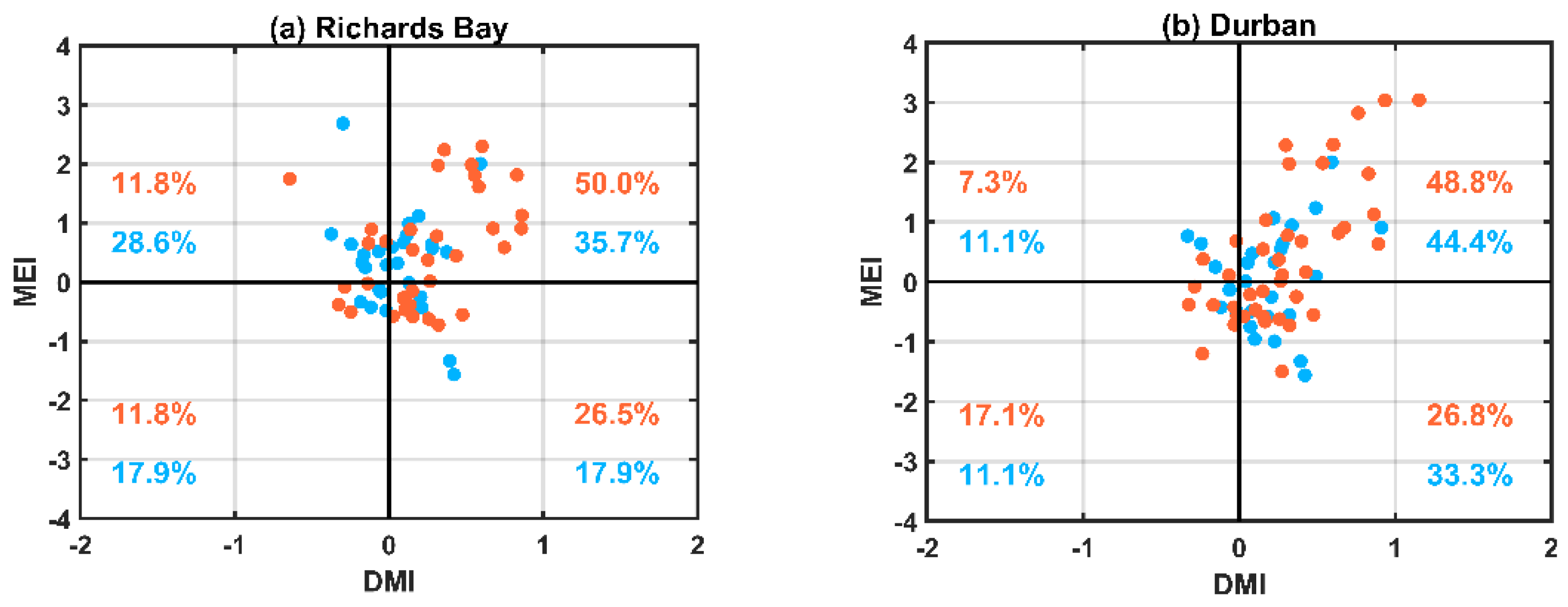
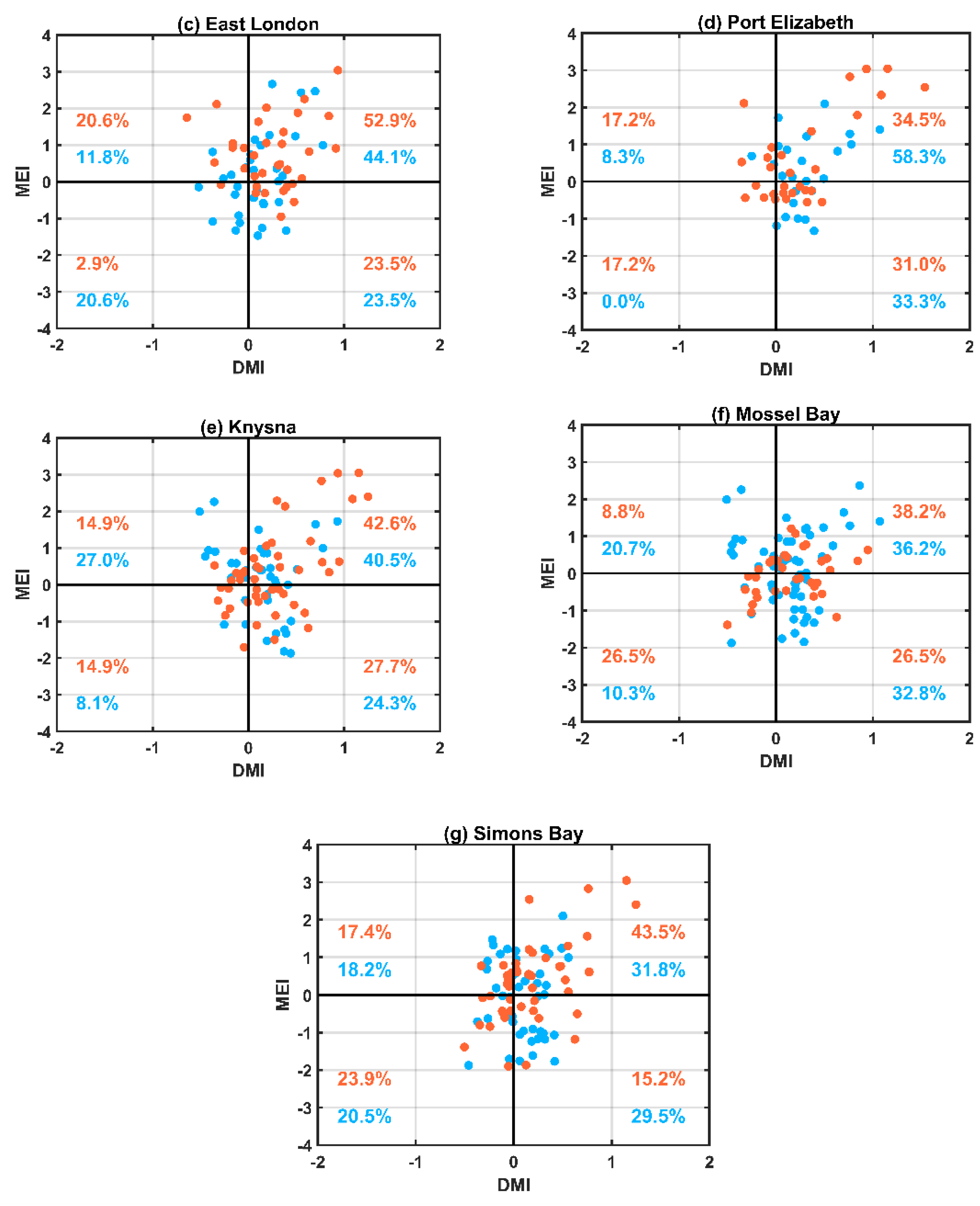
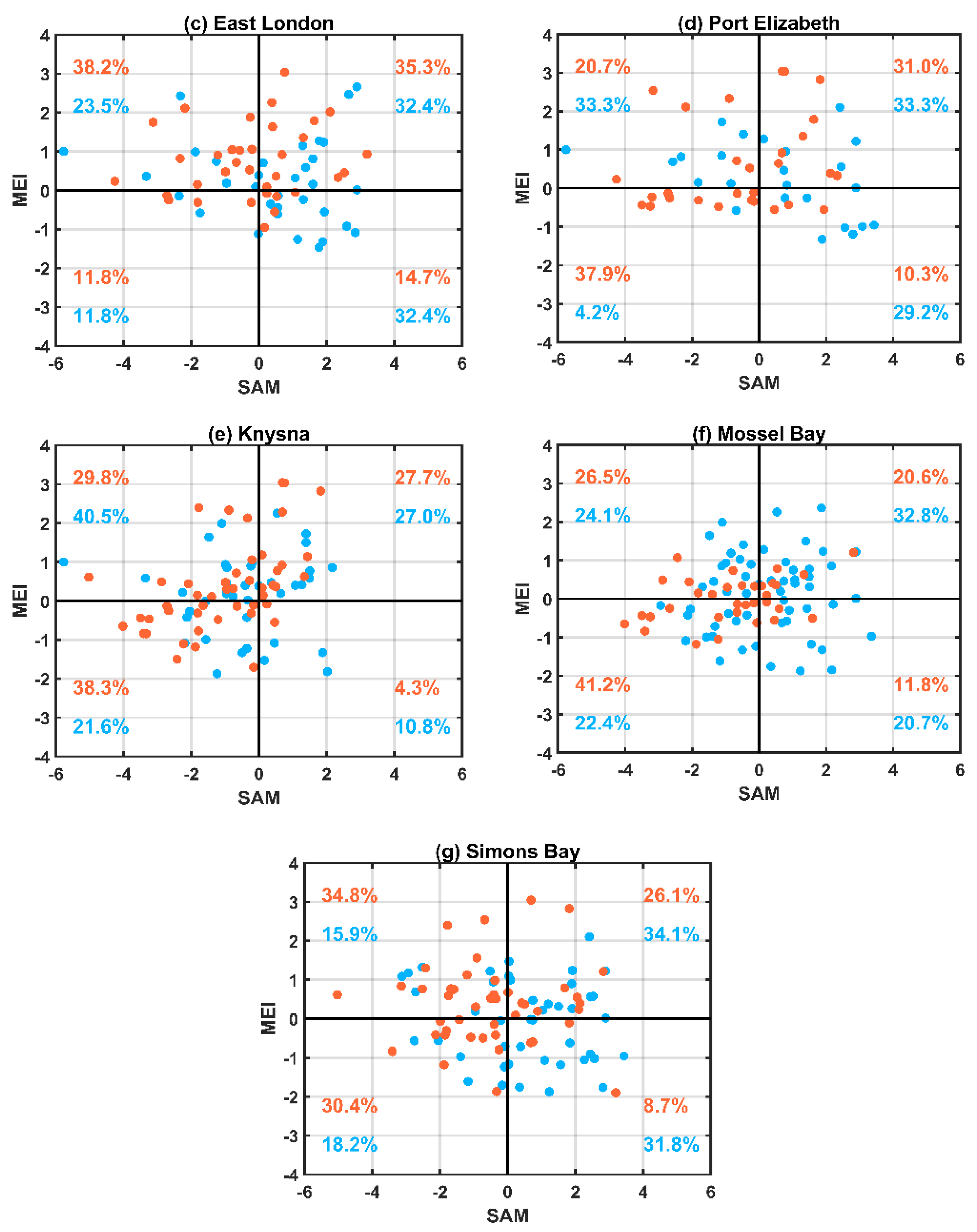
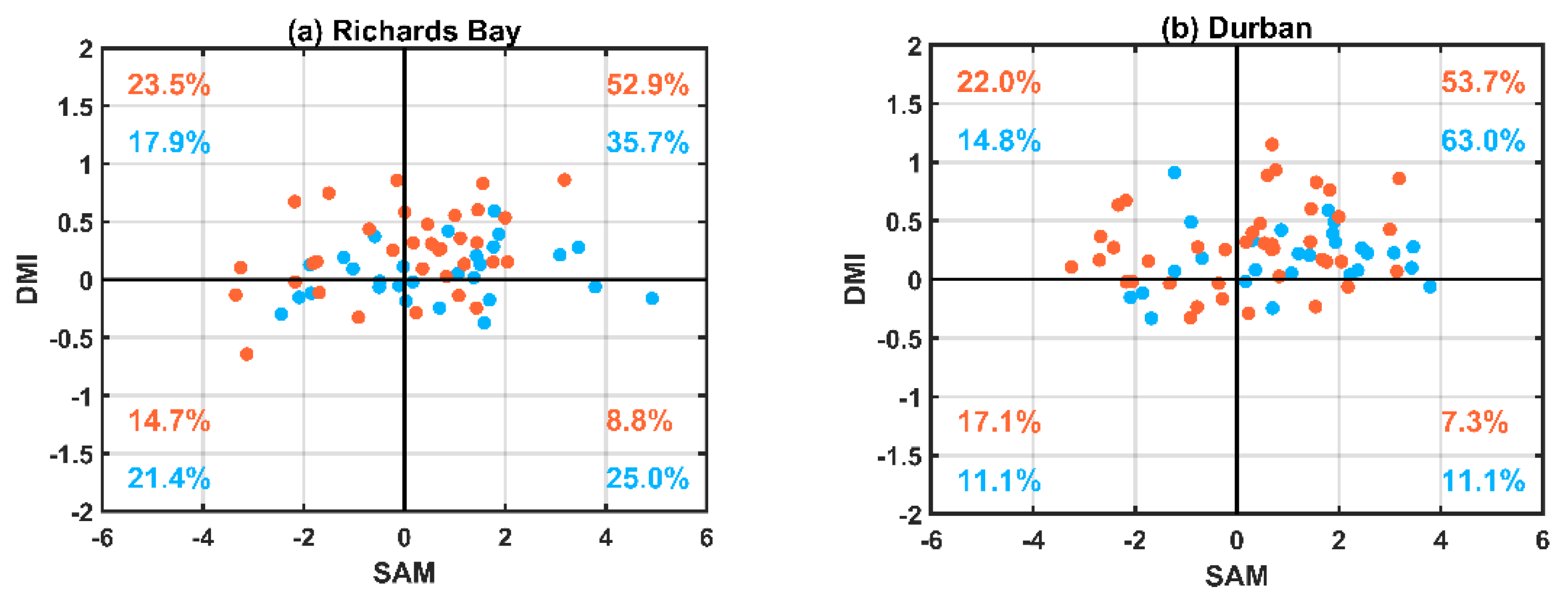
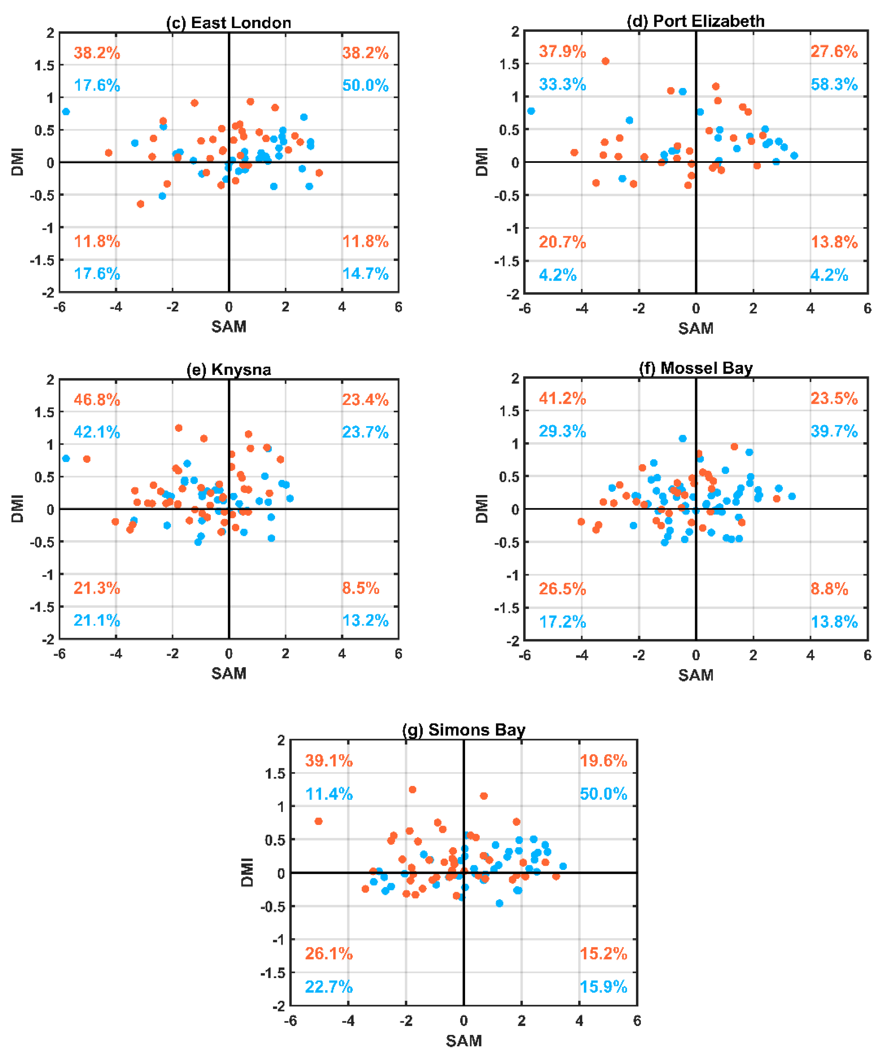
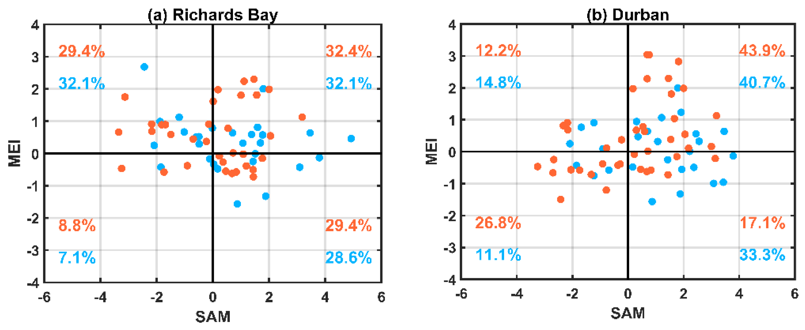
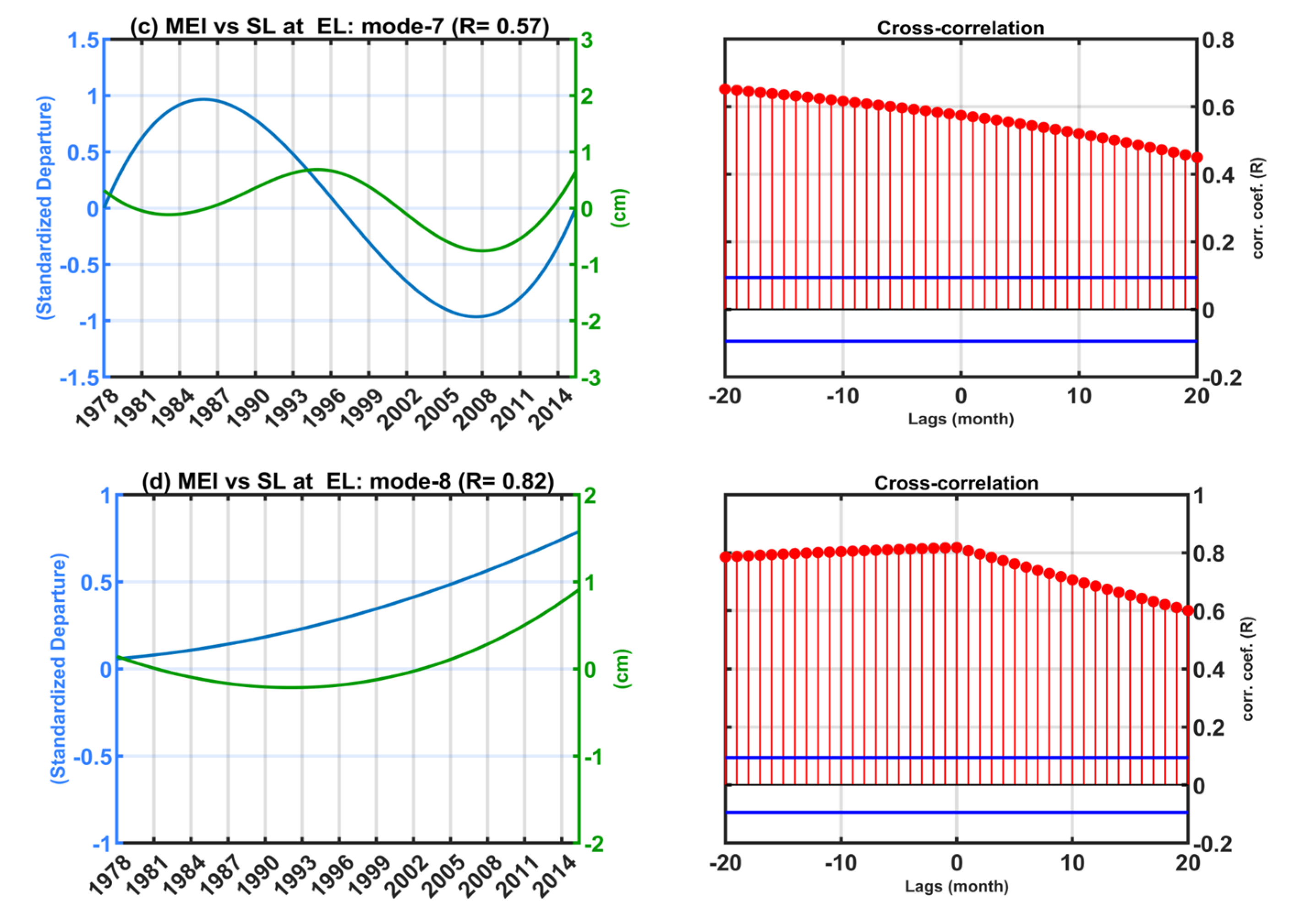
3.2. Drivers of Tide Gauge Sea Level Variability on Interannual Timescales
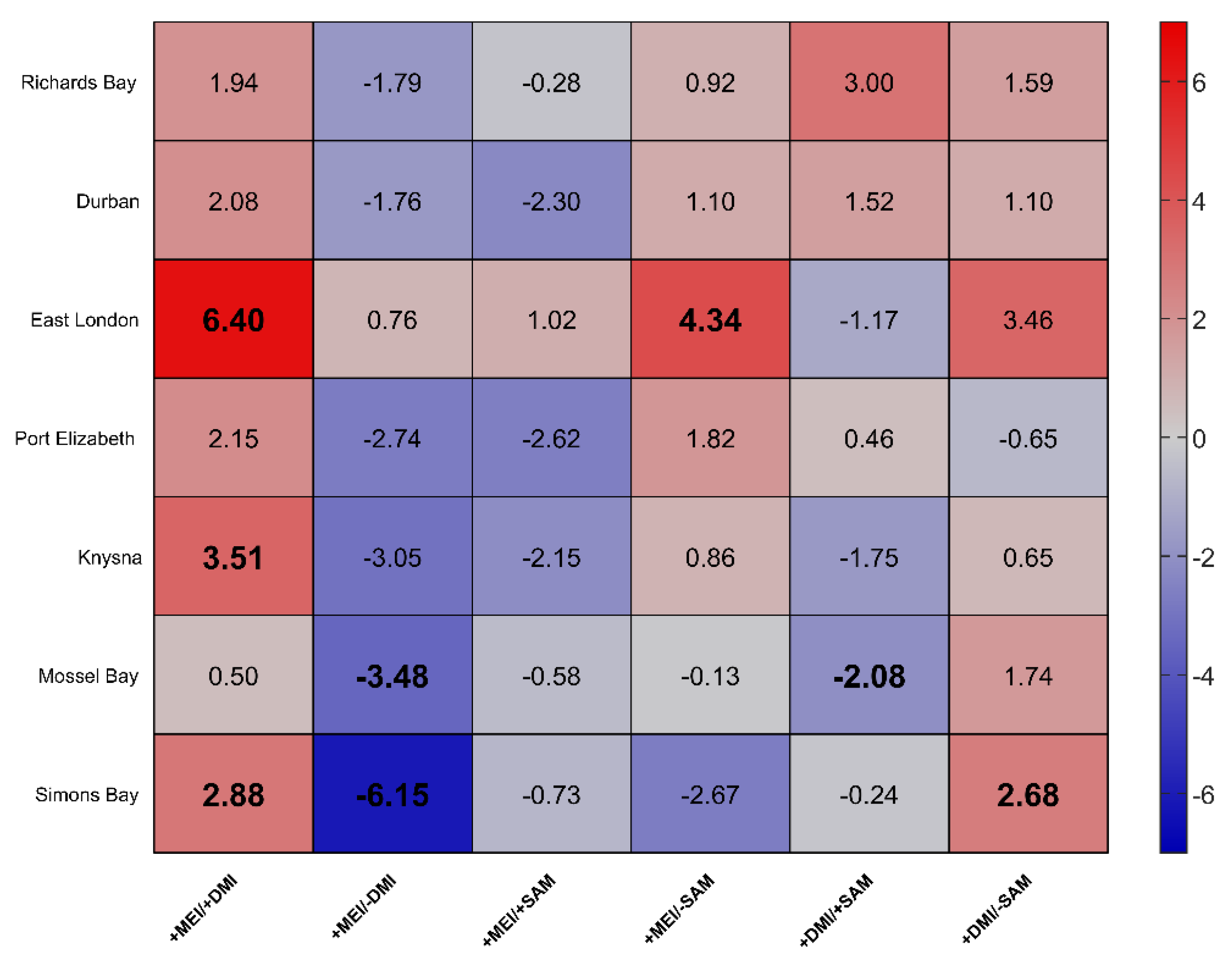
The Combined Influence of the Modes of Climate Variability
4. Discussion
5. Summary and Conclusions
Author Contributions
Funding
Institutional Review Board Statement
Informed Consent Statement
Data Availability Statement
Acknowledgments
Conflicts of Interest
Appendix A


References
- Mather, A.A.; Stretch, D.D.; Garland, G.G. Southern African sea levels: Corrections, influences and trends. Afr. J. Mar. Sci. 2009, 31, 145–156. [Google Scholar] [CrossRef]
- Brundrit, G.B. Monthly Mean Sea Level Variability along the West Coast of Southern Africa. S. Afr. J. Mar. Sci. 1984, 2, 195–203. [Google Scholar] [CrossRef]
- Brundrit, G.B. Trends of Southern African Sea Level: Statistical Analysis and Interpretation. S. Afr. J. Mar. Sci. 1995, 16, 9–17. [Google Scholar] [CrossRef]
- Woodworth, P.L.; Aman, A.; Aarup, T. Sea level monitoring in Africa. Afr. J. Mar. Sci. 2007, 29, 321–330. [Google Scholar] [CrossRef]
- Schumann, E.H. Low frequency fluctuations off the Natal coast. J. Geophys. Res. Oceans 1981, 86, 6499–6508. [Google Scholar] [CrossRef]
- Schumann, E.H. Long-Period Coastal Trapped Waves off the Southeast Coast of Southern Africa. Cont. Shelf Res. 1983, 2, 97–107. [Google Scholar] [CrossRef]
- Brundrit, G.B.; De Cuevas, D.; Shipley, A.M. Significant Sea-Level Variations along the West Coast of Southern Africa 1979–1983. S. Afr. J. Sci. 1984, 80, 80–82. [Google Scholar]
- De Cuevas, B.A.; Brundrit, G.B.; Shipley, A.M. Low-frequency Sea-level Fluctuations along the Coasts of Namibia and South Africa. Geophys. J. R. Astron. Soc. 1986, 87, 33–42. [Google Scholar] [CrossRef] [Green Version]
- Schumann, E.H.; Brink, K.H. Coastal-Trapped Waves off the Coast of South Africa: Generation, Propagation and Current Structures. J. Phys. Oceanogr. 1990, 20, 1206–1218. [Google Scholar] [CrossRef] [Green Version]
- Reason, C.J.C.; Jury, M.R. On the generation and propagation of the southern African coastal low. Q. J. R. Meteorol. Soc. 1990, 116, 1133–1151. [Google Scholar] [CrossRef]
- Weldon, D.; Reason, C.J.C. Variability of rainfall characteristics over the South Coast region of South Africa. Theor. Appl. Climatol. 2014, 115, 177–185. [Google Scholar] [CrossRef]
- Brundrit, G.B.; De Cuevas, B.A.; Shipley, A.M. Long-term sea-level variability in the eastern South Atlantic and a comparison with that in the eastern pacific. S. Afr. J. Mar. Sci. 1987, 5, 73–78. [Google Scholar] [CrossRef]
- Colberg, F.; Reason, C.J.C.; Rodgers, K. South Atlantic response to El Niño-Southern Oscillation induced climate variability in an ocean general circulation model. J. Geophys. Res. C Ocean 2004, 109, 1–14. [Google Scholar] [CrossRef] [Green Version]
- Singleton, A.T.; Reason, C.J.C. Variability in the characteristics of cut-off low pressure systems over subtropical southern Africa. Int. J. Climatol. 2007, 27, 295–310. [Google Scholar] [CrossRef]
- Han, W.; Meehl, G.A.; Rajagopalan, B.; Fasullo, J.T.; Hu, A.; Lin, J.; Large, W.G.; Wang, J.W.; Quan, X.W.; Trenary, L.L.; et al. Patterns of Indian Ocean sea-level change in a warming climate. Nat. Geosci. 2010, 3, 546–550. [Google Scholar] [CrossRef]
- Han, W.; Vialard, J.; McPhaden, M.J.; Lee, T.; Masumoto, Y.; Feng, M.; De Ruijter, W.P.M. Indian ocean decadal variability: A review. Bull. Am. Meteorol. Soc. 2014, 95, 1679–1703. [Google Scholar] [CrossRef]
- Nhantumbo, B.J.; Nilsen, J.E.Ø.; Backeberg, B.C.; Reason, C.J.C. The relationship between coastal sea level variability in South Africa and the Agulhas Current. J. Mar. Syst. 2020, 211, 1–13. [Google Scholar] [CrossRef]
- Huang, N.E.; Shen, Z.; Long, S.R.; Wu, M.C.; Snin, H.H.; Zheng, Q.; Yen, N.C.; Tung, C.C.; Liu, H.H. The empirical mode decomposition and the Hubert spectrum for nonlinear and non-stationary time series analysis. Proc. R. Soc. Lond. Ser. A 1998, 454, 903–995. [Google Scholar] [CrossRef]
- Huang, N.E.; Wu, Z. A Review on Hilbert-Huang Transform: Method and Its Applications. Rev. Geophys. 2008, 46, 1–23. [Google Scholar] [CrossRef] [Green Version]
- Holgate, S.J.; Matthews, A.; Woodworth, P.L.; Rickards, L.J.; Tamisiea, M.E.; Bradshaw, E.; Foden, P.R.; Gordon, K.M.; Jevrejeva, S.; Pugh, J. New Data Systems and Products at the Permanent Service for Mean Sea Level. J. Coast. Res. 2013, 29, 493. [Google Scholar] [CrossRef]
- Kalnay, E.; Kanamitsu, M.; Kistler, R.; Collins, W.; Deaven, D.; Gandin, L. The NCEP/NCAR 40-Year Reanalysis Project. Bull. Am. Meteorol. Soc. 1996, 77, 437–472. [Google Scholar] [CrossRef] [Green Version]
- Huang, B.; Banzon, V.F.; Freeman, E.; Lawrimore, J.; Liu, W.; Peterson, T.C.; Smith, T.M.; Thorne, P.W.; Woodruff, S.D.; Zhang, H.M. Extended reconstructed sea surface temperature version 4 (ERSST.v4). Part I: Upgrades and intercomparisons. J. Clim. 2015, 28, 911–930. [Google Scholar] [CrossRef] [Green Version]
- Saji, N.H.; Goswami, B.N.; Vinayachandran, P.N.; Yamagata, T. A dipole mode in the tropical Indian Ocean. Nature 1999, 401, 360–364. [Google Scholar] [CrossRef]
- Ashok, K.; Guan, Z.; Yamagata, T. Impact of the Indian Ocean Dipole on the Relationship between the Indian Monsoon Rainfall and ENSO. Geophys. Res. Lett. 2001, 28, 4499–4502. [Google Scholar] [CrossRef] [Green Version]
- Hendon, H.H. Indonesian Rainfall Variability: Impacts of ENSO and Local Air-Sea Interaction. J. Clim. 2003, 16, 1775–1790. [Google Scholar] [CrossRef]
- Behera, S.K.; Luo, J.J.; Masson, S.; Delecluse, P.; Gualdi, S.; Navarra, A.; Yamagata, T. Paramount Impact of the Indian Ocean Dipole on the East African Short Rains: A CGCM Study. J. Clim. 2005, 18, 4514–4530. [Google Scholar] [CrossRef] [Green Version]
- Manatsa, D.; Chingombe, W.; Matarira, C.H. The Impact of the Positive Indian Ocean Dipole on Zimbabwe Droughts. Int. J. Climatol. 2008, 28, 2011–2029. [Google Scholar] [CrossRef]
- Manatsa, D.; Matarira, C.H.; Mukwada, G. Relative impacts of ENSO and Indian Ocean dipole/zonal mode on east SADC rainfall. Int. J. Climatol. 2011, 31, 558–577. [Google Scholar] [CrossRef]
- Wolter, K.; Timlin, M.S. Monitoring ENSO in COADS with a seasonally adjusted principal component index. In Proceedings of the 17th Climate Diagnostics Workshop, Norman, OK, USA, 18–23 October 1992; pp. 52–57. [Google Scholar]
- Wolter, K.; Timlin, M.S. Measuring the strength of ENSO events: How does 1997/98 rank? Weather 1998, 53, 315–324. [Google Scholar] [CrossRef]
- Freeman, E.; Woodruff, S.D.; Worley, S.J.; Lubker, S.J.; Kent, E.C.; Angel, W.E.; Berry, D.I.; Brohan, P.; Eastman, R.; Gates, L.; et al. ICOADS Release 3.0: A major update to the historical marine climate record. Int. J. Climatol. 2017, 37, 2211–2232. [Google Scholar] [CrossRef] [Green Version]
- Lindesay, J.A. South African rainfall, the Southern Oscillation and a Southern Hemisphere semi-annual cycle. J. Climatol. 1988, 8, 17–30. [Google Scholar] [CrossRef]
- Reason, C.J.C.; Allan, R.J.; Lindesay, J.A.; Ansell, T.J. Enso and climatic signals across the Indian Ocean basin in the global context: Part I, Interannual composite patterns. Int. J. Climatol. 2000, 20, 1285–1327. [Google Scholar] [CrossRef]
- Marshall, G.J. Trends in the Southern Annular Mode from observations and reanalyses. J. Clim. 2003, 16, 4134–4143. [Google Scholar] [CrossRef]
- Reason, C.J.C.; Rouault, M. Links between the Antarctic Oscillation and winter rainfall over western South Africa. Geophys. Res. Lett. 2005, 32, 1–4. [Google Scholar] [CrossRef]
- Gillett, N.P.; Kell, T.D.; Jones, P.D. Regional climate impacts of the Southern Annular Mode. Geophys. Res. Lett. 2006, 33, 1–4. [Google Scholar] [CrossRef]
- Huang, N.E.; Shen, Z.; Long, S.R. A NEW VIEW OF NONLINEAR WATER WAVES: The Hilbert Spectrum. Annu. Rev. Fluid Mech. 1999, 31, 417–457. [Google Scholar] [CrossRef] [Green Version]
- Ezer, T.; Corlett, W.B. Is sea level rise accelerating in the Chesapeake Bay? A demonstration of a novel new approach for analyzing sea level data. Geophys. Res. Lett. 2012, 39, 1–6. [Google Scholar] [CrossRef] [Green Version]
- Ezer, T.; Atkinson, L.P.; Corlett, W.B.; Blanco, J.L. Gulf Stream’s induced sea level rise and variability along the U.S. mid-Atlantic coast. J. Geophys. Res. Ocean 2013, 118, 685–697. [Google Scholar] [CrossRef] [Green Version]
- Wu, Z.; Huang, N.E. Ensemble empirical mode decomposition: A Noise-Assited. Adv. Adapt. Data Anal. 2009, 1, 1–41. [Google Scholar] [CrossRef]
- Huang, N.E.; Wu, M.L.C.; Long, S.R.; Shen, S.S.P.; Qu, W.; Gloersen, P.; Fan, K.L. A confidence limit for the empirical mode decomposition and Hilbert spectral analysis. Proc. R. Soc. A Math. Phys. Eng. Sci. 2003, 459, 2317–2345. [Google Scholar] [CrossRef]
- Soumya, M.; Vethamony, P.; Tkalich, P. Inter-annual sea level variability in the southern South China Sea. Glob. Planet. Chang. 2015, 133, 17–26. [Google Scholar] [CrossRef]
- Saji, N.H.; Yamagata, T. Possible Impacts of Indian Ocean Dipole Mode Events on Global Climate. Clim. Res. 2003, 25, 151–169. [Google Scholar] [CrossRef]
- Chen, X.; Feng, Y.; Huang, N.E. Global sea level trend during 1993–2012. Glob. Planet. Chang. 2014, 112, 26–32. [Google Scholar] [CrossRef]
- Dangendorf, S.; Calafat, F.M.; Arns, A.; Wahl, T.; Haigh, I.D. Mean Sea Level Variability in the North Sea: Processes and Implications. J. Geophys. Res. Ocean 2014, 119, 6820–6841. [Google Scholar] [CrossRef] [Green Version]
- Park, J.; Sweet, W. Accelerated Sea Level Rise and Florida Current Transport. Ocean Sci. 2015, 11, 607–615. [Google Scholar] [CrossRef] [Green Version]
- Chafik, L.; Nilsen, J.E.Ø.; Dangendorf, S. Impact of North Atlantic teleconnection patterns on northern European sea level. J. Mar. Sci. Eng. 2017, 5, 43. [Google Scholar] [CrossRef] [Green Version]
- Haigh, I.D.; Wahl, T.; Rohling, E.J.; Price, R.M.; Pattiaratchi, C.B.; Calafat, F.M.; Dangendorf, S. Timescales for detecting a significant acceleration in sea level rise. Nat. Commun. 2014, 5, 1–11. [Google Scholar] [CrossRef] [Green Version]
- Zebiak, S.E. Air-sea interaction in the equatorial Atlantic region. J. Clim. 1993, 6, 1567–1586. [Google Scholar] [CrossRef]
- Neelin, J.D.; Battisti, D.S.; Hirst, A.C.; Jin, F.-F.; Wakata, Y.; Yamagata, T.; Zebiak, S.E. ENSO theory. J. Geophys. Res. 1998, 103, 14261–14290. [Google Scholar] [CrossRef]
- Taljaard, J.J. Synoptic Meteorology of the Southern Hemisphere. In Meteorology of the Southern Hemisphere: Meteorological Monographs; Newton, C.W., Ed.; American Meteorological Society: Boston, MA, USA, 1972; Volume 13, pp. 139–213. [Google Scholar] [CrossRef]
- Van Loon, H. Wind in the Southern Hemisphere. In Meteorology of the Southern Hemisphere: Meteorological Monographs; Newton, C.W., Ed.; American Meteorological Society: Boston, MA, USA, 1972; Volume 13, pp. 87–100. [Google Scholar] [CrossRef]
- Preston-Whyte, R.A.; Tyson, P.D. The Atmosphere and Weather of Southern Africa, 1st ed.; Oxford University Press: Cape Town, South Africa, 1988. [Google Scholar]
- Tyson, P.D.; Preston-Whyte, R.A. The Weather and Climate of Southern Africa, 2nd ed.; Oxford University Press: Cape Town, South Africa, 2000. [Google Scholar]
- Pugh, D.T. Tides, Surges and Mean Sea-Level; John Wiley & Sons: Chichester, UK, 1987. [Google Scholar]
- Chelton, D.B.; Davis, R.E. Monthly Mean Sea-Level Variability Along the West Coast of North America. J. Phys. Oceanogr. 1982, 12, 757–784. [Google Scholar] [CrossRef] [Green Version]
- Richter, K.; Segtnan, O.H.; Furevik, T. Variability of the Atlantic Inflow to the Nordic Seas and Its Causes Inferred from Observations of Sea Surface Height. J. Geophys. Res. 2012, 117, 1–12. [Google Scholar] [CrossRef]
- Calafat, F.M.; Chambers, D.P.; Tsimplis, M.N. Inter-annual to decadal sea-level variability in the coastal zones of the Norwegian and Siberian Seas: The role of atmospheric forcing. J. Geophys. Res. Ocean 2013, 118, 1287–1301. [Google Scholar] [CrossRef] [Green Version]
- Woodworth, P.L.; Teferle, F.N.; Bingley, R.M.; Shennan, I.; Williams, S.D.P. Trends in UK mean sea level revisited. Geophys. J. Int. 2009, 176, 19–30. [Google Scholar] [CrossRef] [Green Version]
- Ezer, T.; Haigh, I.D.; Woodworth, P.L. Nonlinear Sea-Level Trends and Long-Term Variability on Western European Coasts. J. Coast. Res. 2016, 320, 744–755. [Google Scholar] [CrossRef]


Publisher’s Note: MDPI stays neutral with regard to jurisdictional claims in published maps and institutional affiliations. |
© 2021 by the authors. Licensee MDPI, Basel, Switzerland. This article is an open access article distributed under the terms and conditions of the Creative Commons Attribution (CC BY) license (https://creativecommons.org/licenses/by/4.0/).
Share and Cite
Nhantumbo, B.J.; Backeberg, B.C.; Nilsen, J.E.Ø.; Reason, C.J.C. Atmospheric and Climatic Drivers of Tide Gauge Sea Level Variability along the East and South Coast of South Africa. J. Mar. Sci. Eng. 2021, 9, 924. https://doi.org/10.3390/jmse9090924
Nhantumbo BJ, Backeberg BC, Nilsen JEØ, Reason CJC. Atmospheric and Climatic Drivers of Tide Gauge Sea Level Variability along the East and South Coast of South Africa. Journal of Marine Science and Engineering. 2021; 9(9):924. https://doi.org/10.3390/jmse9090924
Chicago/Turabian StyleNhantumbo, Bernardino J., Björn C. Backeberg, Jan Even Øie Nilsen, and Chris J. C. Reason. 2021. "Atmospheric and Climatic Drivers of Tide Gauge Sea Level Variability along the East and South Coast of South Africa" Journal of Marine Science and Engineering 9, no. 9: 924. https://doi.org/10.3390/jmse9090924
APA StyleNhantumbo, B. J., Backeberg, B. C., Nilsen, J. E. Ø., & Reason, C. J. C. (2021). Atmospheric and Climatic Drivers of Tide Gauge Sea Level Variability along the East and South Coast of South Africa. Journal of Marine Science and Engineering, 9(9), 924. https://doi.org/10.3390/jmse9090924