Hydrodynamic Behaviour of Floating Polygonal Platforms under Wave Action

Abstract

The hydrodynamic behaviour of floating regular polygonal platforms under wave action was studied by conducting parametric studies. Considering triangular, square, hexagonal, and circular platforms of similar size and draft, the results show that their added mass, radiation damping, and RAOs are similar. However, the wave exciting forces are slightly different, particularly the horizontal forces. The polygonal platforms oriented with one of its corners in line with the prevailing wave direction can lead to a reduction in the horizontal force on the platform, a feature that helps in reducing the cost of a mooring system. Moreover, such oriented platforms are able to disperse the waves better in multiple directions and hence will not pose problems for ships or marine vessels passing by the platform on the weather side. Thus, the orientation of a polygonal platform is an important design consideration. From the comparison study among different polygonal platforms, their wave attenuation performances are slightly similar. The hydrodynamic analyses performed herein for the parametric studies were sped up considerably by using a significantly lesser number of Fourier coefficient sets for the series functions that define the velocity potentials when compared to those used by previous researchers in their analytical approaches. The adoption of the radius function defined by cosine-type radial perturbation does not only generate the geometric boundaries of polygonal platforms, but it also simplifies the formulation and quickens the computations.

1. Introduction

There is considerable interest in using large floating structures for creating land from the sea in land scarce coastal cities and countries. These large floating structures have many advantages over the traditional land reclamation technique, such as being more environmentally friendly to the eco-marine system and cost-effective for birthing land in deep waters [1]. Examples include Monaco’s 352 m long floating jetty/breakwater, which also accommodates car parks and a shopping centre [2]; the Sebit islets, which are artificial floating islands in the Han River of South Korea, which is used for exhibitions, entertainment and leisure activities [3]; Denmark’s floating energy island in the North Sea [4]; the Fjordmax platform for fish farming in Norway [5]; and the Oceanix floating city [6].

Many researchers studied the 3D hydrodynamic analysis of floating structures to understand the interaction between structures and waves with the view to produce optimal floating structure designs and mooring systems. The analyses are generally performed by numerical techniques such as the finite element method (e.g., [7,8]) and the boundary element method (e.g., [9,10]) because they can handle any shape of floating structures or seabed topology. However, such methods require large computational time for solutions and for pre-processing jobs such as mesh discretization. Conversely, analytical methods such as the eigenfunction expansion method can solve hydrodynamic problems of floating structures quickly and furnish accurate results, provided that analytical solutions are available.

In the literature, hydrodynamic problems of different types of floating bodies have been solved analytically. For example, Bhatta and Rahman [11] tackled the diffraction and radiation problems of floating circular cylinders and Yeung [12] obtained the added mass and radiation damping of a vertical cylinder while Chen and Mei [13] addressed floating elliptical cylinders by using the Mathieu function and Williams and Darwiche [14] developed two approximate solutions for the wave radiation by a truncated elliptical cylinder in order to reduce computational efforts. Liu et al. and Yu et al. [15,16] presented a semi-analytical method to handle the diffraction problem and radiation problem of floating arbitrarily shaped cylinders, respectively. By using the semi-analytical method, they investigated the hydrodynamic behaviour of a triangular cosine-type cylinder and a quasi-elliptical cylinder.

Thus far, the hydrodynamic problem of floating polygonal platforms has not been studied analytically, particularly the wave field around the platform. As the incident waves scatter due to the floating platforms and the radiated waves are produced by the platform motion, the resulting wave field may affect other facilities or vessels passing nearby. This paper thus investigates the hydrodynamic behaviour of floating polygonal platforms under wave action. The geometries of regular polygonal platforms were generated by using the cosine-type radial perturbation [17]. Therefore, the formulation for the floating polygonal platforms can be achieved in a straightforward manner. For the hydrodynamic analysis, we developed two improved versions of semi-analytical methods based on Liu et al. [15] quadruple Fourier expansions and Yu et al. [16] triple Fourier expansions. One version is the use of double Fourier expansions, such that it eliminates the need to establish the number of truncated terms for two Fourier expansions. In the second version, quadruple Fourier expansions are still used, but the number of Fourier coefficient sets is reduced to only three when compared to the need for 10 sets in Liu et al. [15] and 16 sets in Yu et al. [16]. This results in a significant reduction of computational time (almost 30% faster). By using the latter version of a semi-analytical approach, 3D hydrodynamic analysis for floating polygonal platforms can be quickened such that parametric studies on hydrodynamic parameters and wave fields can be conducted readily. Hydrodynamic results presented herein include added mass, radiation damping, wave exciting forces, RAOs, wave runup, and wave field in the vicinity of the floating polygonal platforms.

The layout of the paper is as follows. Section 2 articulates the current problem. Section 3 presents the governing equation and boundary conditions for the problem. Section 4 presents the solutions of diffracted and radiated potentials using semi-analytical approaches. Section 5, Section 6 and Section 7 handle the determination of the wave exciting forces, hydrodynamic restoring forces, and motion responses of a floating platform, respectively. Section 8 concerns the verification of the present semi-analytical approaches and compares the computational times required for ANSYS AQWA and the different analytical approaches. In addition, the effective series terms to be considered are presented for a quick calculation of hydrodynamic restoring forces and wave exciting forces. Section 9 presents the hydrodynamic results for different polygonal-shaped platforms. Finally, conclusions are presented in Section 10.

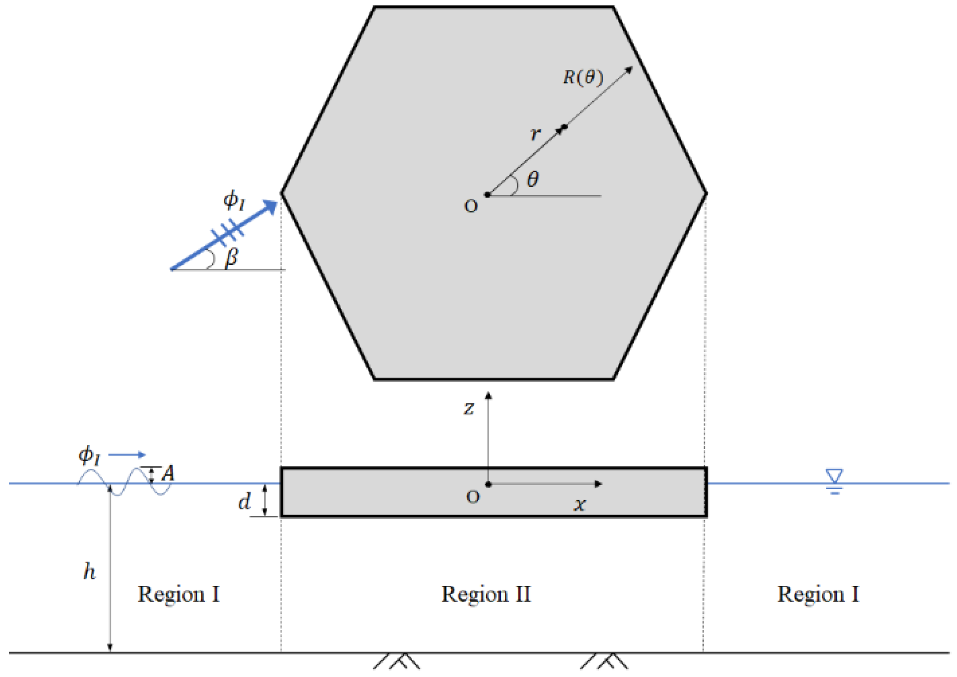
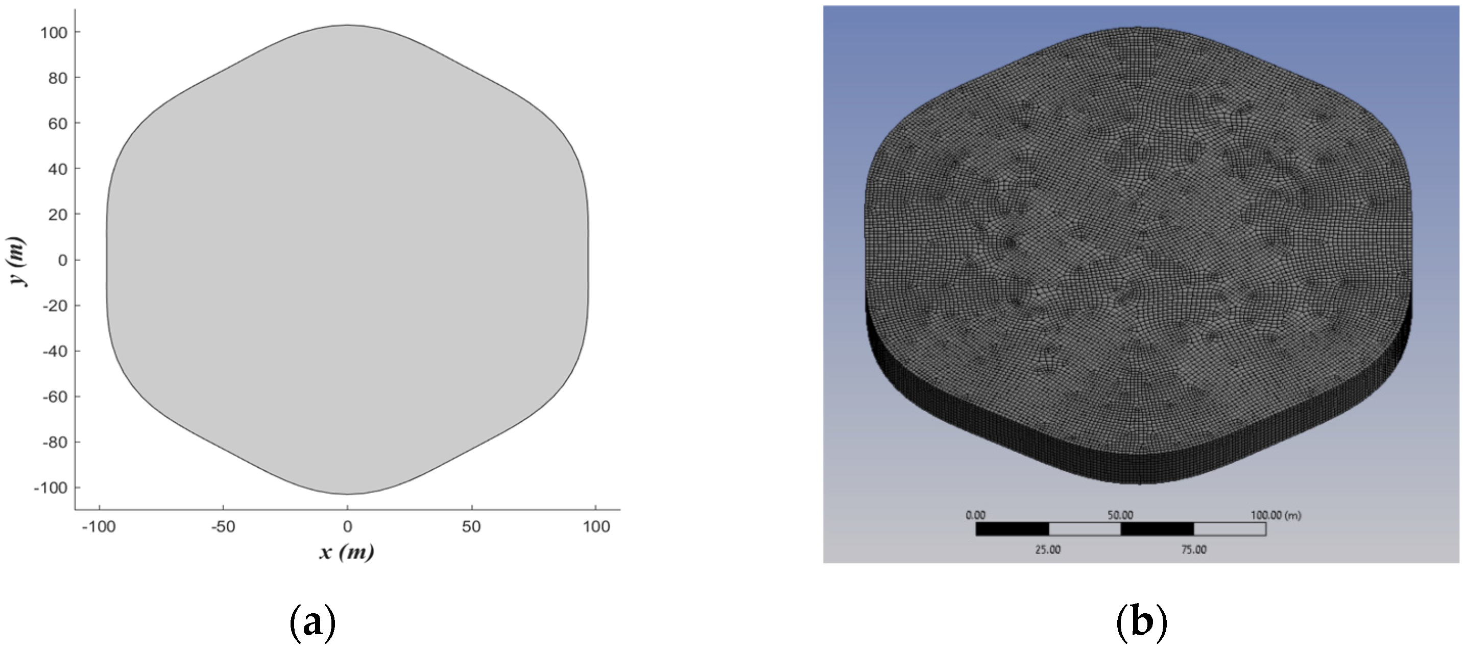
2. Problem Definition

Consider a floating rigid polygonal platform in a constant water depth h as shown in Figure 1. The incident wave has a wave period T, a wave amplitude A, and incidents the floating platform at an oblique angle of β. The freeboard is assumed to be high enough to prevent wave overtopping. The draft of the platform is $d$. The floating platform is allowed to oscillate freely but is assumed to be kept in place. The cylindrical coordinates (r, θ, z) are adopted with its origin at the centre of the regular polygonal platform.

The plan shape of the polygonal platform is generated by using a radius function defined by the cosine-type radial perturbation given by [17].

$$R\left(\theta \right)=R_0\left\{1+\epsilon \cos n_r\left(\theta -{\theta }_0\right)\right\}$$

(1)

where $R_0$, $\epsilon$, $n_r$ and ${\theta }_0$ are parameters to be chosen by a user. This radius function can be used to construct all types of regular polygonal shapes. For example, polygonal shapes such as a triangle, square, pentagon, hexagon and octagon can be straightforwardly created by choosing the appropriate values for the dimensionless parameters $\epsilon$, $n_r$ and ${\theta }_0$, which are summarised in

Table 1. Various regular polygonal shapes created by the cosine-type radial perturbation. (Note: $S_0$ denotes the plan area of platform).

Platform shapes	triangle	square	pentagon	hexagon	octagon
$S_0$	$1.005\times \pi R_0^2$	$1.002\times \mathsf{\pi }{R}_0^2$	$1.001\times \mathsf{\pi }{R}_0^2$	$1.000\times \mathsf{\pi }{R}_0^2$	$1.000\times \mathsf{\pi }{R}_0^2$
$\epsilon$	0.1	0.06	0.04	0.03	0.02
$n_r$	3	4	5	6	8
${\theta }_0$	$\frac{\mathsf{\pi }}{2}$	$\frac{\mathsf{\pi }}{4}$	$\frac{\mathsf{\pi }}{2}$	$\frac{\mathsf{\pi }}{6}$	$\frac{\mathsf{\pi }}{8}$

. The size of the polygonal shape is predominantly controlled by $R_0.$ For a given $R_0$ value, the polygonal shapes have similar plan areas $S_0$ equal to about $\pi R_0^2$; which is convenient when comparing with a circular platform of a similar size. In addition, one can freely orientate the polygonal shape by changing ${\theta }_0$.

The current problem is to determine (i) diffracted and radiated potentials, (ii) wave exciting forces, (iii) added mass, (iv) radiation damping, (v) RAOs (response amplitude operators), (vi) wave runup, and (vii) wave field.

3. Governing Equation and Boundary Conditions

The hydrodynamic analysis will be performed in the frequency domain. The fluid domain is divided into two regions as shown in Figure 1. Region I is the sea space outside the platform domain while Region II is the sea space underneath the platform domain. The fluid is assumed to be incompressible, inviscid and irrotational, and hence the linear potential theory may be applied. Accordingly, the fluid motion is governed by the Laplace equation as

$$\frac{1}{r}\frac{\partial }{\partial r}\left(r\frac{\partial \varphi }{\partial r}\right)+\frac{1}{r^2}\frac{{\partial }^2\varphi }{\partial {\theta }^2}+\frac{{\partial }^2\varphi }{\partial z^2}=0$$

(2)

where $\varphi$ is the velocity potential. This velocity potential can be expressed as the sum of the incident potential ${\varphi }_I$, diffracted potential ${\varphi }_D$, and radiated potential ${\varphi }_R$, i.e.,

$$\varphi ={\varphi }_I+{\varphi }_D+{\varphi }_R$$

(3)

The radiated potential may be expressed as the sum of six radiation modes corresponding to the six degrees of freedom, as

$${\varphi }_R={\displaystyle \sum }_{j=1}^6\left(-i\omega {\xi }_j{\phi }_R^j\right)$$

(4)

where $i$ is the imaginary unit, $\omega$ the wave angular frequency, ${\xi }_j$ the motion amplitude of the platform for the j-th radiation mode, and ${\phi }_R^j$ the normalised radiated potential for the $j$-th radiation mode.

The velocity potential must satisfy the following free surface condition and seabed condition

$${\frac{\partial \varphi }{\partial z}|}_{z=0}={\frac{{\omega }^2}{g}\varphi |}_{z=0} \mathrm{on} \mathrm{the} \mathrm{free} \mathrm{surface}$$

(5)

$${\frac{\partial \varphi }{\partial z}|}_{z=-h}=0\hspace{1em}\mathrm{on} \mathrm{the} \mathrm{seabed}$$

(6)

where $g$ is the gravitational acceleration. The diffracted and radiated potentials must satisfy Sommerfeld’s radiation condition at infinity, that is

$$\underset{r\to \infty }{\lim }\left(\frac{\partial {\varphi }_{D,R}}{\partial r}-ik{\varphi }_{D,R}\right)=0$$

(7)

where k is the wave number. At the wetted surface of the floating platform, the boundary conditions for the diffraction and the radiation problems are, respectively, given by

$$\frac{\partial {\varphi }_D}{\partial n}=-\frac{\partial {\varphi }_I}{\partial n}$$

(8)

$$\frac{\partial {\phi }_R}{\partial n}=n·n_j\hspace{1em}\left(j=1,2,\cdots ,6\right)$$

(9)

where $n$ is the unit normal vector pointing to the wetted surface of the platform and $n_j$ is the generalised motion normal for 6 DOFs (degrees of freedom), i.e., $n_1=n_x$, $n_2=n_y$, $n_3=n_z$, $n_4=-\left(z-z_G\right)n_y+\left(y-y_G\right)n_z$, $n_5=\left(z-z_G\right)n_x-\left(x-x_G\right)n_z$ and $n_6=-\left(y-y_G\right)n_x+\left(x-x_G\right)n_y$, where ($x_G,y_G,z_G)$ are the coordinates of the platform’s centre of gravity. The radial unit normal vector is $n_r=\cos \theta n_x+\sin \theta n_y$, which is used for a circular platform. However, if the radius function with respect to $\theta$ is not constant, the normal derivatives of Equations (8) and (9) must be modified by using the corresponding unit normal vector. Therefore, let us introduce the surface function $S\left(r,\theta \right)=r-R\left(\theta \right)$ and its derivative with respect to $\theta$ defined as $\frac{\partial S}{\partial \theta }=-\frac{\partial R\left(\theta \right)}{\partial \theta }$ [18]. The surface function $S$ implies the distance from the surface of a platform to an arbitrary field point ($r,\theta$) in a given z-plane, which indicates that $S$ is independent on the z-coordinates. A point with positive $S$ is located outside the platform domain while a point with a negative $S$ is located within the platform domain. $S=0$ indicates the associated point is at the edge of the platform domain, which is equivalent to $r=R\left(\theta \right)$. By using the surface function, the unit normal vector pointing to the water $n_s$ is given by [18].

$$n_s=\frac{\nabla S\left(r,\theta \right)}{\left|n_s\right|}=\frac{\frac{\partial S}{\partial r}\overrightarrow{r}+\frac{1}{r}\frac{\partial S}{\partial \theta }\overrightarrow{\theta }+\frac{\partial S}{\partial z}\overrightarrow{z}}{\left|n_s\right|}=\frac{1}{\sqrt{1+{\left(\frac{1}{r}\frac{\partial S}{\partial \theta }\right)}^2}}\left(\overrightarrow{r}+\frac{1}{r}\frac{\partial S}{\partial \theta }\overrightarrow{\theta }+0\overrightarrow{z}\right)$$

(10)

where $\nabla$ denotes the del operator in cylindrical coordinate system for obtaining the gradient of a vector. Thus, the normal velocity on the platform wetted surface in the radial direction can be calculated by using the divergence operator in the cylindrical coordinate system as

$$\nabla \varphi ·n_s=\frac{1}{\sqrt{1+{\left(\frac{1}{r}\frac{\partial S}{\partial \theta }\right)}^2}}\left(\frac{\partial \varphi }{\partial r}+\frac{1}{r^2}\frac{\partial S}{\partial \theta }\frac{\partial \varphi }{\partial \theta }\right)$$

(11)

4. Solutions for Diffracted and Radiated Potentials

The appropriate diffracted or radiated velocity potentials for each region are assumed to be given by [11].

$${\varphi }_1={\displaystyle \sum }_{m=-\infty }^{\infty }\left\{A_{m0}\frac{H_m\left(kr\right)}{H_m\left(ka\right)}\frac{Z_0\left(z\right)}{Z_0\left(0\right)}+{\displaystyle \sum }_{n=1}^{\infty }{A}_{mn}\frac{K_m\left(k_{n}r\right)}{K_m\left(k_{n}a\right)}\frac{Z_n\left(z\right)}{Z_n\left(0\right)}\right\}{e}^{im\theta } \mathrm{for} \mathrm{Region} \mathrm{I}$$

(12)

$${\varphi }_2={\varphi }_{p_2}+{\displaystyle \sum }_{m=-\infty }^{\infty }\left\{B_{m0}{\left(\frac{r}{b}\right)}^{\left|m\right|}+{\displaystyle \sum }_{n=1}^{\infty }{B}_{mn}\frac{I_m\left(p_{n}r\right)}{I_m\left(p_{n}b\right)}\cos p_n\left(z+h\right)\right\}{e}^{im\theta } \mathrm{for} \mathrm{Region} \mathrm{II}$$

(13)

where ${\varphi }_{p_2}$ is the particular solution and the vertical eigenfunction $Z_n$for Region I is given by

$$Z_0\left(z\right)=\frac{\cosh k\left(z+h\right)}{\sqrt{N_0}},\hspace{1em}{N}_0=\frac{1}{2}\left[1+\frac{\sinh 2kh}{2kh}\right],\left(n=0\right)$$

(14)

$$Z_n\left(z\right)=\frac{\cos k_n\left(z+h\right)}{\sqrt{N_n}},\hspace{1em}{N}_n=\frac{1}{2}\left[1+\frac{\sin 2k_{n}h}{2k_{n}h}\right],\left(n=1,2,\cdots ,\infty \right)$$

(15)

$A_{mn}$ and $B_{mn}$are the unknown complex coefficients to be determined; $I_m$ and $K_m$ are respectively the modified Bessel function of the first and the second kinds of order $m$; $a$ and $b$ are respectively the shortest and the longest distance from the origin to the platform surface along the radial direction, which may be calculated from the radius function $R\left(\theta \right).$ $\mathrm{The} \mathrm{wavenumber} k$, and the vertical eigenvalue $k_n$ for Region I are given by

$$\frac{{\omega }^2}{g}-k\tanh k=0$$

(16)

$$k_0=-ik,\hspace{1em}\frac{{\omega }^2}{g}+k_n\tan k_n=0\left(n=1,2,\infty \right)$$

(17)

and vertical eigenvalue $p_n$ for Region II is given by

$$p_n=\frac{\pi n}{h-d} \left(n=0,1,2,\infty \right)$$

(18)

The particular solution must satisfy governing Equation (2), the seabed condition Equation (6), and the wetted surface boundary conditions Equations (8) and (9) in the vertical direction, i.e.,

$$\frac{\partial {\phi }_{p_2}^{\left(j\right)}}{\partial z}=n_z·n_j={\delta }_{3j}+\left(y-y_G\right){\delta }_{4j}-\left(x-x_G\right){\delta }_{5j} \mathrm{on} z=-d$$

(19)

where ${\delta }_{ij}$ is the Kronecker delta (1 if $i=j$ and 0 if $i\ne j$).

For the diffraction problem, ${\varphi }_{p_2}=-{\varphi }_I$ and for the radiation problem, ${\phi }_{p_2}^{\left(j\right)}$ is given by

$${\phi }_{p_2}^{\left(j\right)}\left(r,\theta ,z\right)=\frac{4{\left(z+h\right)}^2-\left(1+{\delta }_{3j}\right)r^2}{8\left(h-d\right)}\left\{{\delta }_{3j}+{\delta }_{4j}\left(r\sin \theta -y_G\right)-{\delta }_{5j}\left(r\cos \theta -x_G\right)\right\}$$

(20)

where the subscript or the superscript $j$ denotes the radiation mode.

The incident velocity potential in the cylindrical coordinate system is given by

$${\varphi }_I\left(r,\theta ,z\right)=-\frac{igA}{\omega }{\displaystyle \sum }_{m=-\infty }^{\infty }{J}_m\left(kr\right)e^{im\left(\theta +\frac{\pi }{2}-\beta \right)}\frac{\cosh k\left(z+h\right)}{\cosh kh}$$

(21)

where $g$ is the gravitational acceleration, $A$ the wave amplitude, $\beta$ the oblique angle of the incident waves, and $J_m$ the Bessel function of the first kind of order $m$.

The matching conditions for the pressure and velocity continuities for the diffraction problem are

$$\nabla {\varphi }_{D_1}·n_s=\{\begin{array}{c}-\nabla {\varphi }_I·n_s\\ \nabla {\varphi }_{D_2}·n_s\end{array} \mathrm{at} r=R \mathrm{and} \{\begin{array}{c}-d\le z\le 0\\ -h\le z\le -d\end{array}$$

(22)

$${\varphi }_{D_2}={\varphi }_{D_1} \mathrm{at} r=R \mathrm{and} -h\le z\le -d$$

(23)

where $R$ denotes the radius function with respect to the angular coordinates$R\left(\theta \right)$. For calculating the divergence operator in Equation (22), one can refer to Equation (11). The denominator of Equation (11) may be cancelled out and $r^2$ may be multiplied on both sides of Equation (22) to remove the fractional terms.

The matching conditions for the pressure and velocity continuities for the radiation problem are

$$\nabla {\phi }_{R_1}^j·n_s=\{\begin{array}{c}{n}_j·n_s\\ \nabla {\phi }_{R_2}^j·n_s\end{array} \mathrm{at} r=R \mathrm{and} \{\begin{array}{c}-d\le z\le 0\\ -h\le z\le -d\end{array}$$

(24)

$${\phi }_{R_2}^j={\phi }_{R_1}^j \mathrm{at} r=R \mathrm{and} -h\le z\le -d$$

(25)

In order to calculate $n_j·n_s$ of Equation (24), another form of the unit normal vector $n_s$ in the Cartesian coordinate system may be needed, which is given by

$$n_s=\frac{\nabla S\left(r,\theta \right)}{\left|n_s\right|}=\frac{\frac{\partial S}{\partial x}\overrightarrow{x}+\frac{\partial S}{\partial y}\overrightarrow{y}+\frac{\partial S}{\partial z}\overrightarrow{z}}{\left|n_s\right|}=\frac{1}{\sqrt{1+{\left(\frac{1}{r}\frac{\partial S}{\partial \theta }\right)}^2}}\left\{\left(\cos \theta -\frac{\sin \theta }{r}\frac{\partial S}{\partial \theta }\right)\overrightarrow{x}+\left(\sin \theta +\frac{\cos \theta }{r}\frac{\partial S}{\partial \theta }\right)\overrightarrow{y}+0\overrightarrow{z}\right\}$$

(26)

One can obtain the six normalised radiation velocity components of the platform at $r=R\left(\theta \right)$ by applying the divergence operator (see Appendix A).

4.1. Solution for Diffraction Problem

For brevity, we consider the horizontal coordinates of the centre of gravity to coincide with the origin, i.e., $\left(x_G,y_G\right)=\left(0, 0\right)$, but the vertical coordinate of the centre of gravity is not zero, $z_G\ne 0$. For diffraction problems, the assumed velocity potentials given in Equations (12), (13) and (21) are substituted into the matching conditions given in Equations (22) and (23). This furnishes

$$\begin{gathered} \begin{array}{c}{\displaystyle {\displaystyle \sum }_{m=-\infty }^{\infty }}{\displaystyle {\displaystyle \sum }_{n=0}^{\infty }}{A}_{mn}{K_{mn}^{\prime }\left(r\right)|}_{r=R\left(\theta \right)}\exp \left(im\theta \right)\frac{Z_n\left(z\right)}{Z_n\left(0\right)}\hfill \\ =\frac{igA}{\omega \cosh kh}{\displaystyle {\displaystyle \sum }_{m=-\infty }^{\infty }}{e}^{im\left(\frac{\pi }{2}-\beta \right)}{J_{m0}^{\prime }\left(r\right)|}_{r=R\left(\theta \right)}\exp \left(im\theta \right)\cosh k\left(z+h\right)\hfill \end{array} \\ \left(-d\le z\le 0, 0\le \theta \le 2\pi \right) \end{gathered}$$

(27)

$$\begin{gathered} \begin{array}{c}{\displaystyle {\displaystyle \sum }_{m=-\infty }^{\infty }}{\displaystyle {\displaystyle \sum }_{n=0}^{\infty }}{A}_{mn}{K_{mn}^{\prime }\left(r\right)|}_{r=R\left(\theta \right)}\exp \left(im\theta \right)\frac{Z_n\left(z\right)}{Z_n\left(0\right)}-{\displaystyle {\displaystyle \sum }_{m=-\infty }^{\infty }}{\displaystyle {\displaystyle \sum }_{n=0}^{\infty }}{B}_{mn}{I_{mn}^{\prime }\left(r\right)|}_{r=R\left(\theta \right)}\exp \left(im\theta \right)\cos p_n\left(z+h\right)\hfill \\ =\frac{igA}{\omega \cosh kh}{\displaystyle {\displaystyle \sum }_{m=-\infty }^{\infty }}{e}^{im\left(\frac{\pi }{2}-\beta \right)}{J_{m0}^{\prime }\left(r\right)|}_{r=R\left(\theta \right)}\exp \left(im\theta \right)\cosh k\left(z+h\right)\hfill \end{array} \\ \left(-h\le z\le -d, 0\le \theta \le 2\pi \right) \end{gathered}$$

(28)

$$\begin{gathered} \begin{array}{c}{\displaystyle {\displaystyle \sum }_{m=-\infty }^{\infty }}{\displaystyle {\displaystyle \sum }_{n=0}^{\infty }}{A}_{mn}{K_{mn}\left(r\right)|}_{r=R\left(\theta \right)}\exp \left(im\theta \right)\frac{Z_n\left(z\right)}{Z_n\left(0\right)}-{\displaystyle {\displaystyle \sum }_{m=-\infty }^{\infty }}{\displaystyle {\displaystyle \sum }_{n=0}^{\infty }}{B}_{mn}{I_{mn}\left(r\right)|}_{r=R\left(\theta \right)}\exp \left(im\theta \right)\cos p_n\left(z+h\right)\hfill \\ =\frac{igA}{\omega \cosh kh}{\displaystyle {\displaystyle \sum }_{m=-\infty }^{\infty }}{e}^{im\left(\frac{\pi }{2}-\beta \right)}{J_m\left(kr\right)|}_{r=R\left(\theta \right)}\exp \left(im\theta \right)\cosh k\left(z+h\right)\hfill \end{array} \\ \left(-h\le z\le -d, 0\le \theta \le 2\pi \right) \end{gathered}$$

(29)

where $K_{mn}$, $I_{mn}$, $K_{mn}^{\prime }$, $I_{mn}^{\prime }$ and $J_{m0}^{\prime }$ are given by for $n=0$,

$$K_{m0}\left(r\right)=\frac{H_m\left(kr\right)}{H_m\left(ka\right)},\hspace{1em}{I}_{m0}\left(r\right)={\left(\frac{r}{b}\right)}^{\left|m\right|}$$

(30)

$$K_{m0}^{\prime }\left(r\right)=r^2\frac{H_m^{\prime }\left(kr\right)}{H_m\left(ka\right)}+im\frac{\partial S}{\partial \theta }\frac{H_m\left(kr\right)}{H_m\left(ka\right)},\hspace{1em}{I}_{m0}^{\prime }\left(r\right)=r^2\frac{\left|m\right|}{b}{\left(\frac{r}{b}\right)}^{\left|m\right|-1}+im\frac{\partial S}{\partial \theta }{\left(\frac{r}{b}\right)}^{\left|m\right|}$$

(31)

$$J_{m0}^{\prime }\left(r\right)=r^2{J}_m^{\prime }\left(kr\right)+im\frac{\partial S}{\partial \theta }{J}_m\left(kr\right)$$

(32)

for $n>0$,

$$K_{mn}\left(r\right)=\frac{K_m\left(k_{n}r\right)}{K_m\left(k_{n}a\right)}, I_{mn}\left(r\right)=\frac{I_m\left(p_{n}r\right)}{I_m\left(p_{n}b\right)}$$

(33)

$$K_{mn}^{\prime }\left(r\right)=r^2\frac{K_m^{\prime }\left(k_{n}r\right)}{K_m\left(k_{n}a\right)}+im\frac{\partial S}{\partial \theta }\frac{K_m\left(k_{n}r\right)}{K_m\left(k_{n}a\right)}, I_{mn}^{\prime }\left(r\right)=r^2\frac{I_m^{\prime }\left(p_{n}r\right)}{I_m\left(p_{n}b\right)}+im\frac{\partial S}{\partial \theta }\frac{I_m\left(p_{n}r\right)}{I_m\left(p_{n}b\right)}$$

(34)

${K_m}^{\prime }$, ${I_m}^{\prime }$, ${H_m}^{\prime }$, and ${J_m}^{\prime }$ denote derivatives with respect to $r$ of $K_m$, $I_m$, $H_m$, and $J_m$, respectively.

4.2. Solution for Radiation Problem

For radiation problems, we substitute Equations (12), (13) and (20) into Equations (24) and (25) to obtain

$$\begin{gathered} {\displaystyle \sum }_{m=-\infty }^{\infty }{\displaystyle \sum }_{n=0}^{\infty }{A}_{mn}^{\left(j\right)}{K_{mn}^{\prime }\left(r\right)|}_{r=R\left(\theta \right)}\exp \left(im\theta \right)\frac{Z_n\left(z\right)}{Z_n\left(0\right)}=R^2\sqrt{1+\frac{S_{\theta }^2}{R^2}}{f_R^{\left(j\right)}\left(r,\theta ,z\right)|}_{r=R\left(\theta \right)} \\ \left(-d\le z\le 0, 0\le \theta \le 2\pi \right) \end{gathered}$$

(35)

$$\begin{gathered} {\left.{\displaystyle \sum }_{m=-\mathrm{\infty }}^{\mathrm{\infty }} {\displaystyle \sum }_{n=0}^{\mathrm{\infty }} A_{mn}^{(j)}{K}_{mn}^{\prime }(r)\right|}_{r=R(\theta )}\exp (im\theta )\frac{Z_n(z)}{Z_n(0)}-{\left.{\displaystyle \sum }_{m=-\mathrm{\infty }}^{\mathrm{\infty }} {\displaystyle \sum }_{n=0}^{\mathrm{\infty }} B_{mn}^{(j)}{I}_{mn}^{\prime }(r)\right|}_{r=R(\theta )}\exp (im\theta )\cos p_n(z+h)={\left.R^2\sqrt{1+\frac{s_{\theta }^2}{R^2}}{\phi }_{p_2}^{(j)}(r,\theta ,z)\right|}_{r=R(\theta )} \\ \left(-h\le z\le -d, 0\le \theta \le 2\pi \right) \end{gathered}$$

(36)

$$\begin{gathered} {\displaystyle \sum }_{m=-\infty }^{\infty }{\displaystyle \sum }_{n=0}^{\infty }{A}_{mn}^{\left(j\right)}{K_{mn}\left(r\right)|}_{r=R\left(\theta \right)}\exp \left(im\theta \right)\frac{Z_n\left(z\right)}{Z_n\left(0\right)}-{\displaystyle \sum }_{m=-\infty }^{\infty }{\displaystyle \sum }_{n=0}^{\infty }{B}_{mn}^{\left(j\right)}{I_{mn}\left(r\right)|}_{r=R\left(\theta \right)}\exp \left(im\theta \right)\cos p_n\left(z+h\right)={{\phi }_{p_2}^{\left(j\right)}\left(r,\theta ,z\right)|}_{r=R\left(\theta \right)} \\ \left(-h\le z\le -d, 0\le \theta \le 2\pi \right) \end{gathered}$$

(37)

where $S_{\theta }$ denotes $\frac{\partial S}{\partial \theta }$. $K_{mn}$, $I_{mn}$, $K_{mn}^{\prime }$, $I_{mn}^{\prime }$ are given in Equations (30), (31), (33) and (34), $f_R^{\left(j\right)}\left(r,\theta ,z\right)$ in Appendix A and ${\phi }_{p_2}^{\left(j\right)}\left(r,\theta ,z\right)$ in Equation (20). ${{\phi }_{p_2}^{{\left(j\right)}^{\prime }}\left(r,\theta ,z\right)|}_{r=R\left(\theta \right)}$can be obtained by substituting the particular solutions of the radiation problem into Equation (11). Thus, one has

$${{\phi }_{p_2}^{{\left(3\right)}^{\prime }}\left(r,\theta ,z\right)|}_{r=R\left(\theta \right)}=-\frac{R}{2\left(h-d\right)\sqrt{1+\frac{S_{\theta }^2}{R^2}}}$$

(38)

$${{\phi }_{p_2}^{{\left(4\right)}^{\prime }}\left(r,\theta ,z\right)|}_{r=R\left(\theta \right)}=\frac{4{\left(z+h\right)}^2\left(\sin \theta +\frac{\cos \theta }{R}{S}_{\theta }\right)-R^2\left(3\sin \theta +\frac{\cos \theta }{R}{S}_{\theta }\right)}{8\left(h-d\right)\sqrt{1+\frac{S_{\theta }^2}{R^2}}}$$

(39)

$${{\phi }_{p_2}^{{\left(5\right)}^{\prime }}\left(r,\theta ,z\right)|}_{r=R\left(\theta \right)}=-\frac{4{\left(z+h\right)}^2\left(\cos \theta -\frac{\sin \theta }{R}{S}_{\theta }\right)-R^2\left(3\cos \theta -\frac{\sin \theta }{R}{S}_{\theta }\right)}{8\left(h-d\right)\sqrt{1+\frac{S_{\theta }^2}{R^2}}}$$

(40)

By multiplying the corresponding vertical eigenfunctions $\frac{1}{h}{Z}_n\left(z\right)$ and $\frac{1}{h-d}\cos p_n\left(z+h\right)$ and the angular eigenfunction $e^{-im\theta }$ in Equations (27)–(29), Equations (35)–(37) and integrating the equations for the associated integral intervals, one can combine Equation (27) with (28) and (35) with (36), respectively. By truncating the series terms at $m=M$ and $n=N$, $2\left(2M+1\right)\left(N+1\right)$ equations and unknowns are given for the diffraction problem and each radiation mode. Consequently, the unknown complex coefficients ($A_{mn}$, $B_{mn}$, $A_{mn}^{\left(j\right)}$, $B_{mn}^{\left(j\right)}$) can be solved by the linear algebra. The functions describing the incoming waves ($r^{\left|m\right|}$ and $I_m$) diverge at the far-field, whereas the functions describing the outgoing waves ($H_m$ and $K_m$) diverge at the near-field. Hence, when the numerical integration is conducted, slightly inaccurate results may be obtained, or the integration may take considerable time to satisfy the required accuracy. In order to avoid these problems, those functions were normalised as given in Equations (30)–(34) by applying the longest distance $b$ to the incoming waves and the shortest distance $a$ to the outgoing waves.

Note that in view of an arbitrary radius function that describes the platform plan geometry, the integration cannot be performed analytically, and thus numerical integration must be resorted. This approach will be referred herein as semi-analytical approach 1.

Liu et al. [15] replaced the radial terms expressed by the radius function with the Fourier expansion series such that the integration can be performed analytically. However, the approach in Liu et al. [15] suffers the following drawbacks:

• the quadruple summation series are required as compared to semi-analytical approach 1, which only requires double summation series;
• the Fourier coefficients must be numerically calculated in advance;
• the convergence analysis is required to determine the truncation numbers of additional series ($N_r$ and $Q$).

$N_r$-series represents the radius function R(θ) while $Q$-series represents the radial functions with respect to r. These radial functions include the Bessel function, Hankel function, the modified Bessel functions and exponential function. If the geometry of the platform is complicated, more $N_r$- and $Q$-series terms may be required, which will increase the computational effort considerably.

A significant contribution of the present study is the reduction of Liu et al. [15] 10 sets of Fourier coefficients for solving the diffraction problem and Yu et al. [16] 16 sets of Fourier coefficients for solving the radiation problem to only three sets such as $a_{m,n,q}$, $b_{m,n,q}$ and $f_{m,q}$ for determining the diffracted and radiated potentials. As a result, it leads to a significant reduction in computational effort and mitigates the abovementioned drawbacks. This second approach will be referred to as semi-analytical approach 2. The applied Fourier expansions used in semi-analytical approach 2 are given by

$${H_m\left(kr\right)|}_{r=R\left(\theta \right)}={\displaystyle \sum }_{q=-\infty }^{\infty }{a}_{m,0,q}{e}^{iq\theta } \left(n=0\right)$$

(41)

$${K_m\left(k_{n}r\right)|}_{r=R\left(\theta \right)}={\displaystyle \sum }_{q=-\infty }^{\infty }{a}_{m,n,q}{e}^{iq\theta } \left(n=1,2,\cdots ,\infty \right)$$

(42)

$${r^{\left|m\right|}|}_{r=R\left(\theta \right)}={\displaystyle \sum }_{q=-\infty }^{\infty }{b}_{m,0,q}{e}^{iq\theta } \left(n=0\right)$$

(43)

$${I_m\left(p_{n}r\right)|}_{r=R\left(\theta \right)}={\displaystyle \sum }_{q=-\infty }^{\infty }{b}_{m,n,q}{e}^{iq\theta } \left(n=1,2,\cdots ,\infty \right)$$

(44)

$${J_m\left(kr\right)|}_{r=R\left(\theta \right)}={\displaystyle \sum }_{q=-\infty }^{\infty }{f}_{m,q}{e}^{iq\theta }$$

(45)

The derivatives with respect to $r$ of Equations (41)–(45) can be directly obtained by using $a_{m,n,q}$, $b_{m,n,q}$ and $f_{m,q}$, i.e.,

$${H_m^{\prime }\left(kr\right)|}_{r=R\left(\theta \right)}=\frac{k}{2}{\displaystyle \sum }_{q=-\infty }^{\infty }\left(a_{m-1,0,q}-a_{m+1,0,q}\right)e^{iq\theta } \left(n=0\right)$$

(46)

$${K_m^{\prime }\left(k_{n}r\right)|}_{r=R\left(\theta \right)}=-\frac{k_n}{2}{\displaystyle \sum }_{q=-\infty }^{\infty }\left(a_{m-1,n,q}+a_{m+1,n,q}\right)e^{iq\theta } \left(n=1,2,\cdots ,\infty \right)$$

(47)

$${\left|m\right|r^{\left|m\right|-1}|}_{r=R\left(\theta \right)}=\frac{1}{r}\left|m\right|{\displaystyle \sum }_{q=-\infty }^{\infty }{b}_{m,0,q}{e}^{iq\theta } \left(n=0\right)$$

(48)

$${I_m^{\prime }\left(p_{n}r\right)|}_{r=R\left(\theta \right)}=+\frac{p_n}{2}{\displaystyle \sum }_{q=-\infty }^{\infty }\left(b_{m-1,n,q}+b_{m+1,n,q}\right)e^{iq\theta } \left(n=1,2,\cdots ,\infty \right)$$

(49)

$${J_m^{\prime }\left(kr\right)|}_{r=R\left(\theta \right)}=\frac{k}{2}{\displaystyle \sum }_{q=-\infty }^{\infty }\left(f_{m-1,q}-f_{m+1,q}\right)e^{iq\theta }$$

(50)

The radius function and the derivative of surface function with respect to $\theta$ can be obtained by using $b_{m,0,q}$.

$${r|}_{r=R\left(\theta \right)}={\displaystyle \sum }_{n_r=-\infty }^{\infty }{b}_{1,0,n_r}{e}^{i{n}_r\theta }$$

(51)

$${\frac{\partial S}{\partial \theta }|}_{S=0}=-{\displaystyle \sum }_{n_r=-\infty }^{\infty }\left(i{n}_r\right)b_{1,0,n_r}{e}^{i{n}_r\theta }$$

(52)

The foregoing derivatives (Equations (46)–(50)) have the same coefficients as in Equations (41)–(45). In contrast, Liu et al. [15] derivatives have a different set of coefficients. As a result of this smaller number of coefficients for semi-analytical approach 2, the computational time is significantly reduced.

The necessary normal derivatives for solution can now be expressed in terms of the coefficients $a_{m,n,q}$, $b_{m,n,q}$ and $f_{m,q}$, as

$$\begin{array}{c}{R}^2{H}_m^{\prime }\left(kR\right)+im{S}_{\theta }{H}_m\left(kR\right)\hfill \\ ={\displaystyle {\displaystyle \sum }_{n_r=-\infty }^{\infty }}{\displaystyle {\displaystyle \sum }_{q=-\infty }^{\infty }}\left\{\frac{k}{2}{b}_{2,0n_r}\left(a_{m-1,0,q}-a_{m+1,0,q}\right)+m{n}_r{b}_{1,0,n_r}{a}_{m,0,q}\right\}{e}^{i\left(n_r+q\right)\theta }\hfill \end{array}$$

(53)

$$\begin{array}{c}{R}^2{K}_m^{\prime }\left(k_{n}R\right)+im{S}_{\theta }{K}_m\left(k_{n}R\right)\hfill \\ ={\displaystyle {\displaystyle \sum }_{n_r=-\infty }^{\infty }}{\displaystyle {\displaystyle \sum }_{q=-\infty }^{\infty }}\left\{-\frac{k_n}{2}{b}_{2,0n_r}\left(a_{m-1,n,q}+a_{m+1,n,q}\right)+m{n}_r{b}_{1,0,n_r}{a}_{m,n,q}\right\}{e}^{i\left(n_r+q\right)\theta }\hfill \end{array}$$

(54)

$$\begin{array}{c}{R}^2\left|m\right|R^{\left|m\right|-1}+im{S}_{\theta }{R}^{\left|m\right|}\hfill \\ ={\displaystyle {\displaystyle \sum }_{q=-\infty }^{\infty }}\left\{\left|m\right|b_{1,0,n_r}{b}_{m,0,q}+m{n}_r{b}_{1,0,n_r}{b}_{m,0,q}\right\}{e}^{i\left(n_r+q\right)\theta }\hfill \end{array}$$

(55)

$$\begin{array}{c}{R}^2{I}_m^{\prime }\left(p_{n}R\right)+im{S}_{\theta }{I}_m\left(p_{n}R\right)\hfill \\ ={\displaystyle {\displaystyle \sum }_{n_r=-\infty }^{\infty }}{\displaystyle {\displaystyle \sum }_{q=-\infty }^{\infty }}\left\{\frac{p_n}{2}{b}_{2,0n_r}\left(b_{m-1,n,q}+b_{m+1,n,q}\right)+m{n}_r{b}_{1,0,n_r}{b}_{m,n,q}\right\}{e}^{i\left(n_r+q\right)\theta }\hfill \end{array}$$

(56)

$$\begin{array}{c}{R}^2{J}_m^{\prime }\left(kR\right)+im{S}_{\theta }{J}_m\left(kR\right)\hfill \\ ={\displaystyle {\displaystyle \sum }_{n_r=-\infty }^{\infty }}{\displaystyle {\displaystyle \sum }_{q=-\infty }^{\infty }}\left\{\frac{k}{2}{b}_{2,0n_r}\left(f_{m-1,q}-f_{m+1,q}\right)+m{n}_r{b}_{1,0,n_r}{f}_{m,q}\right\}{e}^{i\left(n_r+q\right)\theta }\hfill \end{array}$$

(57)

By substituting Equations (41)–(57) into Equations (27)–(29) for the diffraction problem, one obtains

$$\begin{gathered} \begin{array}{c}\begin{array}{cc}{\displaystyle {\displaystyle \sum }_{m=-\mathrm{\infty }}^{\mathrm{\infty }}}{\displaystyle {\displaystyle \sum }_{n_r=-\mathrm{\infty }}^{\mathrm{\infty }}}{\displaystyle {\displaystyle \sum }_{q=-\mathrm{\infty }}^{\mathrm{\infty }}}\hfill & \left[\frac{A_{m0}}{H_m(ka)}\left\{\frac{k}{2}{b}_{2,0,n_r}\left(a_{m-1,0,q}-a_{m+1,0,q}\right)\right.\right.\hfill \\ & \left.+m{n}_r{b}_{1,0,n_r}{a}_{m,0,q}\right\}\frac{Z_0(z)}{Z_0(0)}\hfill \\ & +{\displaystyle {\displaystyle \sum }_{n=1}^{\mathrm{\infty }}} \frac{A_{mn}}{K_m\left(k_{n}a\right)}\left\{-\frac{k_n}{2}{b}_{2,0,n_r}\left(a_{m-1,n,q}+a_{m+1,n,q}\right)\right.\hfill \\ & \left.\left.+m{n}_r{b}_{1,0,n_r}{a}_{m,n,q}\right\}\frac{Z_n(z)}{Z_n(0)}\right]e^{i\left(m+n_r+q\right)\theta }\hfill \end{array}\hfill \\ =\frac{igA\cosh k\left(z+h\right)}{\omega \cosh kh}{\displaystyle {\displaystyle \sum }_{m=-\infty }^{\infty }}{e}^{im\left(\frac{\pi }{2}-\beta \right)}{\displaystyle {\displaystyle \sum }_{n_r=-\infty }^{\infty }}{\displaystyle {\displaystyle \sum }_{q=-\infty }^{\infty }}\left\{\frac{k}{2}{b}_{2,0,n_r}\left(f_{m-1,q}-f_{m+1,q}\right)+m{n}_r{b}_{1,0,n_r}{f}_{m,q}\right\}{e}^{i\left(m+n_r+q\right)\theta }\hfill \end{array} \\ \left(-d\le z\le 0, 0\le \theta \le 2\pi \right) \end{gathered}$$

(58)

$$\begin{gathered} \begin{array}{c}\begin{array}{cc}{\displaystyle {\displaystyle \sum }_{m=-\mathrm{\infty }}^{\mathrm{\infty }}}{\displaystyle {\displaystyle \sum }_{n_r=-\mathrm{\infty }}^{\mathrm{\infty }}}{\displaystyle {\displaystyle \sum }_{q=-\mathrm{\infty }}^{\mathrm{\infty }}}\hfill & \left[\frac{A_{m0}}{H_m(ka)}\left\{\frac{k}{2}{b}_{2,0,n_r}\left(a_{m-1,0,q}-a_{m+1,0,q}\right)\right.\right.\hfill \\ & \left.+m{n}_r{b}_{1,0,n_r}{a}_{m,0,q}\right\}\frac{Z_0(z)}{Z_0(0)}\hfill \\ & +{\displaystyle {\displaystyle \sum }_{n=1}^{\mathrm{\infty }}} \frac{A_{mn}}{K_m\left(k_{n}a\right)}\left\{-\frac{k_n}{2}{b}_{2,0,n_r}\left(a_{m-1,n,q}+a_{m+1,n,q}\right)\right.\hfill \\ & \left.\left.+m{n}_r{b}_{1,0,n_r}{a}_{m,n,q}\right\}\frac{Z_n(z)}{Z_n(0)}\right]e^{i\left(m+n_r+q\right)\theta }\hfill \\ -{\displaystyle {\displaystyle \sum }_{m=-\mathrm{\infty }}^{\mathrm{\infty }}}{\displaystyle {\displaystyle \sum }_{n_r=-\mathrm{\infty }}^{\mathrm{\infty }}}{\displaystyle {\displaystyle \sum }_{q=-\mathrm{\infty }}^{\mathrm{\infty }}}\hfill & \left[\frac{B_{m0}}{b^{|m|}}\left\{|m|b_{1,0,n_r}{b}_{m,0,q}+m{n}_r{b}_{1,0,n_r}{b}_{m,0,q}\right\}\right.\hfill \\ & +{\displaystyle {\displaystyle \sum }_{n=1}^{\mathrm{\infty }}}\frac{B_{mn}}{I_m\left(p_{n}b\right)}\left\{\frac{p_n}{2}{b}_{2,0,n_r}\left(b_{m-1,n,q}+b_{m+1,n,q}\right)\right.\hfill \\ & \left.\left.+m{n}_r{b}_{1,0,n_r}{b}_{m,n,q}\right\}\cos p_n(z+h)\right]e^{i\left(m+n_r+q\right)\theta }\hfill \end{array}\hfill \\ =\frac{igA\cosh k\left(z+h\right)}{\omega \cosh kh}{\displaystyle {\displaystyle \sum }_{m=-\infty }^{\infty }}{e}^{im\left(\frac{\pi }{2}-\beta \right)}{\displaystyle {\displaystyle \sum }_{n_r=-\infty }^{\infty }}{\displaystyle {\displaystyle \sum }_{q=-\infty }^{\infty }}\left\{\frac{k}{2}{b}_{2,0,n_r}\left(f_{m-1,q}-f_{m+1,q}\right)+m{n}_r{b}_{1,0,n_r}{f}_{m,q}\right\}{e}^{i\left(m+n_r+q\right)\theta }\hfill \end{array} \\ \left(-h\le z\le -d, 0\le \theta \le 2\pi \right) \end{gathered}$$

(59)

$$\begin{gathered} \begin{array}{c}{\displaystyle {\displaystyle \sum }_{m=-\mathrm{\infty }}^{\mathrm{\infty }}}{\displaystyle {\displaystyle \sum }_{q=-\mathrm{\infty }}^{\mathrm{\infty }}}\left\{\frac{A_{m0}}{H_m(ka)}{a}_{m,0,q}\frac{Z_0(z)}{Z_0(0)}+{\displaystyle {\displaystyle \sum }_{n=1}^{\mathrm{\infty }}}\frac{A_{mn}}{K_m\left(k_{n}a\right)}{a}_{m,n,q}\frac{Z_n(z)}{Z_n(0)}\right\}{e}^{i(m+q)\theta }-{\displaystyle {\displaystyle \sum }_{m=-\mathrm{\infty }}^{\mathrm{\infty }}}{\displaystyle {\displaystyle \sum }_{q=-\mathrm{\infty }}^{\mathrm{\infty }}}\left\{\frac{B_{m0}}{b^{\left|m\right|}}{b}_{m,0q}+{\displaystyle {\displaystyle \sum }_{n=1}^{\mathrm{\infty }}}\frac{B_{mn}}{I_m\left(p_{n}b\right)}{b}_{m,nq}\cos p_n(z+h)\right\}{e}^{i(m+q)\theta }\hfill \\ =\frac{igA\cosh k\left(z+h\right)}{\omega \cosh kh}{\displaystyle {\displaystyle \sum }_{m=-\infty }^{\infty }}{e}^{im\left(\frac{\pi }{2}-\beta \right)}{\displaystyle {\displaystyle \sum }_{q=-\infty }^{\infty }}{f}_{m,q}{e}^{i\left(m+q\right)\theta }\hfill \end{array} \\ \left(-h\le z\le -d, 0\le \theta \le 2\pi \right) \end{gathered}$$

(60)

By comparing Equations (27)–(34) of semi-analytical approach 1 with Equations (58)–(60) of semi-analytical approach 2, it can be seen that the latter set of equations for the solution is more complicated but obtaining the solution is faster.

By substituting Equations (42)–(57) into Equations (35)–(37) for the radiation problem, one obtains

$$\begin{gathered} \begin{array}{c}\begin{array}{cc}{\displaystyle {\displaystyle \sum }_{m=-\mathrm{\infty }}^{\mathrm{\infty }}}{\displaystyle {\displaystyle \sum }_{n_r=-\mathrm{\infty }}^{\mathrm{\infty }}}{\displaystyle {\displaystyle \sum }_{q=-\mathrm{\infty }}^{\mathrm{\infty }}}& \left[\frac{A_{m0}^{(j)}}{H_m(ka)}\left\{\frac{k}{2}{b}_{2,0,n_r}\left(a_{m-1,0,q}-a_{m+1,0,q}\right)\right.\right.\hfill \\ & \left.+m{n}_r{b}_{1,0,n_r}{a}_{m,0,q}\right\}\frac{Z_0(z)}{Z_0(0)}\hfill \\ & +{\displaystyle {\displaystyle \sum }_{n=1}^{\mathrm{\infty }}}\frac{A_{mn}^{(j)}}{K_m\left(k_{n}a\right)}\left\{-\frac{k_n}{2}{b}_{2,0,n_r}\left(a_{m-1,n,q}+a_{m+1,n,q}\right)\right.\hfill \\ & \left.\left.+m{n}_r{b}_{1,0,n_r}{a}_{m,n,q}\right\}\frac{Z_n(z)}{Z_n(0)}\right]e^{i\left(m+n_r+q\right)\theta }\hfill \end{array}\hfill \\ =R^2\sqrt{1+\frac{S_{\theta }^2}{R^2}}{f_R^{\left(j\right)}\left(r,\theta ,z\right)|}_{r=R\left(\theta \right)}\hfill \end{array} \\ \left(-d\le z\le 0, 0\le \theta \le 2\pi \right) \end{gathered}$$

(61)

$$\begin{gathered} \begin{array}{c}\begin{array}{cc}\hfill {\displaystyle {\displaystyle \sum }_{m=-\mathrm{\infty }}^{\mathrm{\infty }}}{\displaystyle {\displaystyle \sum }_{n_r=-\mathrm{\infty }}^{\mathrm{\infty }}}{\displaystyle {\displaystyle \sum }_{q=-\mathrm{\infty }}^{\mathrm{\infty }}}& \left[\frac{A_{m0}^{(j)}}{H_m(ka)}\left\{\frac{k}{2}{b}_{2,0,n_r}\left(a_{m-1,0,q}-a_{m+1,0,q}\right)\right.\right.\hfill \\ & \left.+m{n}_r{b}_{1,0,n_r}{a}_{m,0,q}\right\}\frac{Z_0(z)}{Z_0(0)}\hfill \\ & +{\displaystyle {\displaystyle \sum }_{n=1}^{\mathrm{\infty }}}\frac{A_{mn}^{(j)}}{K_m\left(k_{n}a\right)}\left\{-\frac{k_n}{2}{b}_{2,0,n_r}\left(a_{m-1,n,q}+a_{m+1,n,q}\right)\right.\hfill \\ & \left.\left.+m{n}_r{b}_{1,0,n_r}{a}_{m,n,q}\right\}\frac{Z_n(z)}{Z_n(0)}\right]e^{i\left(m+n_r+q\right)\theta }\hfill \\ \hfill -{\displaystyle {\displaystyle \sum }_{m=-\mathrm{\infty }}^{\mathrm{\infty }}}{\displaystyle {\displaystyle \sum }_{r=-\mathrm{\infty }}^{\mathrm{\infty }}}{\displaystyle {\displaystyle \sum }_{q=-\mathrm{\infty }}^{\mathrm{\infty }}}& \left[\frac{B_{m0}^{(j)}}{b^{|m|}}\left\{|m|b_{1,0,n_r}{b}_{m,0,q}+m{n}_r{b}_{1,0,n_r}{b}_{m,0,q}\right\}\right.\hfill \\ & +{\displaystyle {\displaystyle \sum }_{n=1}^{\mathrm{\infty }}} \frac{B_{mn}^{(j)}}{I_m\left(p_{n}b\right)}\left\{\frac{p_n}{2}{b}_{2,0,n_r}\left(b_{m-1,n,q}+b_{m+1,n,q}\right)\right.\hfill \\ & \left.\left.+m{n}_r{b}_{1,0,n_r}{b}_{m,n,q}\right\}\cos p_n(z+h)\right]e^{i\left(m+n_r+q\right)\theta }\hfill \end{array}\hfill \\ =R^2\sqrt{1+\frac{S_{\theta }^2}{R^2}}{{\phi }_{p_2}^{{\left(j\right)}^{\prime }}\left(r,\theta ,z\right)|}_{r=R\left(\theta \right)}\hfill \end{array} \\ \left(-h\le z\le -d, 0\le \theta \le 2\pi \right) \end{gathered}$$

(62)

$$\begin{gathered} \begin{array}{c}{\displaystyle {\displaystyle \sum }_{m=-\mathrm{\infty }}^{\mathrm{\infty }}}{\displaystyle {\displaystyle \sum }_{q=-\mathrm{\infty }}^{\mathrm{\infty }}}\left\{\frac{A_{m0}}{H_m(ka)}{a}_{m,0,q}\frac{Z_0(z)}{Z_0(0)}+{\displaystyle {\displaystyle \sum }_{n=1}^{\mathrm{\infty }}} \frac{A_{mn}}{K_m\left(k_{n}a\right)}{a}_{m,n,q}\frac{Z_n(z)}{Z_n(0)}\right\}{e}^{i(m+q)\theta }-{\displaystyle {\displaystyle \sum }_{m=-\mathrm{\infty }}^{\mathrm{\infty }}}{\displaystyle {\displaystyle \sum }_{q=-\mathrm{\infty }}^{\mathrm{\infty }}}\left\{\frac{B_{m0}}{b^{\left|m\right|}}{b}_{m,0,q}+{\displaystyle {\displaystyle \sum }_{n=1}^{\mathrm{\infty }}} \frac{B_{mn}}{I_m\left(p_{n}b\right)}{b}_{m,n,q}\cos p_n(z+h)\right\}{e}^{i(m+q)\theta }\hfill \\ ={{\phi }_{p_2}^{\left(j\right)}\left(r,\theta ,z\right)|}_{r=R\left(\theta \right)}\hfill \end{array} \\ \left(-h\le z\le -d, 0\le \theta \le 2\pi \right) \end{gathered}$$

(63)

The detailed expressions for $R^2\sqrt{1+\frac{S_{\theta }^2}{R^2}}{f_R^{\left(j\right)}\left(r,\theta ,z\right)|}_{r=R\left(\theta \right)}$, $R^2\sqrt{1+\frac{S_{\theta }^2}{R^2}}{{\phi }_{p_2}^{{\left(j\right)}^{\prime }}\left(r,\theta ,z\right)|}_{r=R\left(\theta \right)}$ and ${{\phi }_{p_2}^{\left(j\right)}\left(r,\theta ,z\right)|}_{r=R\left(\theta \right)}$ and other useful expressions are given in Appendix B. Similarly to semi-analytical approach 1, the corresponding vertical eigenfunctions $\frac{1}{h}{Z}_n\left(z\right)$ and $\frac{1}{h-d}\cos p_n\left(z+h\right)$ and the angular eigenfunction $e^{-im\theta }$ are multiplied in Equations (58)–(63) and integrating the equations for the associated integral intervals, one can combine Equation (58) with (59) and (61) with (62), respectively. By truncating the series terms at $m=M$, n = N, $n_r=N_r$ and $q=Q$, $2\left(2M+1\right)\left(N+1\right)$ equations and unknowns are given for the diffraction problem and each radiation mode. Consequently, the unknown complex coefficients ($A_{mn}$, $B_{mn}$, $A_{mn}^{\left(j\right)}$, $B_{mn}^{\left(j\right)}$) can be solved by the linear algebra.

By comparing Equations (35)–(40) of semi-analytical approach 1 with Equations (61)–(63) of semi-analytical approach 2, it can be seen that the latter set of equations for solution is more complicated but obtaining the solution is faster.

5. Determination of Wave Exciting Force

From the Bernoulli’s equation, the fluid pressure p is

$$p=\rho i\omega \varphi$$

(64)

where $\rho$ is the water density.

By integrating over the wetted areas $S_w$, the wave exciting force and rotational moment for six DOFs are obtained by

$$F_{w_j}=\rho i\omega \underset{S_w}{\overset{}{{\displaystyle \int }}}\left({\varphi }_I+{\varphi }_D\right)·n_j\mathrm{d}{S}_w$$

(65)

Considering the oblique incident wave angle $\beta =0$ and symmetrical geometry of platform about x-axis, the problem becomes simpler as we need to handle only three DOFs. Thus, the wave exciting forces in the x- and z-axis $\mathrm{are} F_{w_1}$ (surge force), $F_{w_3}$ (heave force), and rotational moment about the y-axis $F_{w_5}$ (pitch moment) are only needed to be calculated. Their expressions are given below:

$$\begin{gathered} F_{w_1}=\rho i\omega \underset{S_w}{\overset{}{{\displaystyle \int }}}\left({\varphi }_I+{\varphi }_D\right)·n_1\mathrm{d}{S}_w=\rho i\omega {{\displaystyle \int }}_0^{2\pi }{{\displaystyle \int }}_{-d}^0{\left({\varphi }_I+{\varphi }_{D_1}\right)|}_{r=R}{n}_x·\left(-n_s\right)R\mathrm{d}z\mathrm{d}\theta \\ =-\frac{\rho gA}{\cosh kh}{\displaystyle \sum }_{m=-\infty }^{\infty }{e}^{im\left(\frac{\pi }{2}-\beta \right)}{{\displaystyle \int }}_0^{2\pi }{J}_m\left(kR\right)e^{im\theta }\frac{R\cos \theta -\sin \theta {\mathrm{S}}_{\theta }}{\sqrt{1+{\left(\frac{S_{\theta }}{R}\right)}^2}} \mathrm{d}\theta {{\displaystyle \int }}_{-d}^0\cosh k\left(z+h\right)\mathrm{d}z \\ -\rho i\omega {\displaystyle \sum }_{m=-\infty }^{\infty }{\displaystyle \sum }_{n=0}^{\infty }{A}_{mn}{{\displaystyle \int }}_0^{2\pi }{K}_{mn}\left(R\right)e^{im\theta }\frac{R\cos \theta -\sin \theta {\mathrm{S}}_{\theta }}{\sqrt{1+{\left(\frac{S_{\theta }}{R}\right)}^2}}\mathrm{d}\theta {{\displaystyle \int }}_{-d}^0\frac{Z_n\left(z\right)}{Z_n\left(0\right)}\mathrm{d}z \end{gathered}$$

(66)

$$\begin{gathered} F_{w_3}=\rho i\omega {{\displaystyle \int }}_{S_w}^{}\left({\varphi }_I+{\varphi }_D\right)·n_3\mathrm{d}{S}_w=\rho i\omega {{\displaystyle \int }}_0^{2\pi }{{\displaystyle \int }}_0^R{\left({\varphi }_I+{\varphi }_{D_2}\right)|}_{z=-d}{n}_z·\left(n_z\right)r\mathrm{d}r\mathrm{d}\theta \\ =\rho i\omega {\displaystyle \sum }_{m=-\infty }^{\infty }{\displaystyle \sum }_{n=0}^{\infty }{B}_{mn}\cos p_n\left(h-d\right){{\displaystyle \int }}_0^{2\pi }{{\displaystyle \int }}_0^R{I}_{mn}\left(r\right)e^{im\theta }r\mathrm{d}r\mathrm{d}\theta \end{gathered}$$

(67)

$$\begin{array}{c}{F}_{w_5}=\rho i\omega {{\displaystyle \int }}_{S_w}^{}\left({\varphi }_I+{\varphi }_D\right)n_5\mathrm{d}{S}_w\hfill \\ =\rho i\omega {{\displaystyle \int }}_0^{2\pi }\left\{{{\displaystyle \int }}_{-d}^0{\left({\varphi }_I+{\varphi }_{D_1}\right)|}_{r=R}\left(z-z_G\right)n_x·\left(-n_s\right)R\mathrm{d}z-{{\displaystyle \int }}_0^R{\left({\varphi }_I+{\varphi }_{D_2}\right)|}_{z=-d}\left(r\cos \theta \right)n_z·\left(n_z\right)r\mathrm{d}r\right\}\mathrm{d}\theta \hfill \\ =-\frac{\rho gA}{\cosh kh}{\displaystyle {\displaystyle \sum }_{m=-\infty }^{\infty }}{e}^{im\left(\frac{\pi }{2}-\beta \right)}\left\{{{\displaystyle \int }}_0^{2\pi }{J}_m\left(kR\right)e^{im\theta }\frac{R\cos \theta -\sin \theta {\mathrm{S}}_{\theta }}{\sqrt{1+{\left(\frac{S_{\theta }}{R}\right)}^2}}\mathrm{d}\theta {{\displaystyle \int }}_{-d}^0\left(z-z_G\right)\cosh k\left(z+h\right)\mathrm{d}z+\cosh k\left(h-d\right){{\displaystyle \int }}_0^{2\pi }{{\displaystyle \int }}_0^R{J}_m\left(kr\right)e^{im\theta }{r}^2\cos \theta \mathrm{d}r\mathrm{d}\theta \right\}\hfill \\ -\rho i\omega {\displaystyle {\displaystyle \sum }_{m=-\mathrm{\infty }}^{\mathrm{\infty }}}{\displaystyle {\displaystyle \sum }_{n=0}^{\mathrm{\infty }}}\left\{A_{mn}{{\displaystyle \int }}_0^{2\pi } K_{mn}(R)e^{im\theta }\frac{R\cos \theta -\sin \theta S_{\theta }}{{\sqrt{1+\left(\frac{S_{\theta }}{R}\right)}}^2}\mathrm{d}\theta {{\displaystyle \int }}_{-d}^0 \left(z-z_G\right)\frac{Z_n(z)}{Z_n(0)}\mathrm{d}z+B_{mn}\cos p_n(h-d){{\displaystyle \int }}_0^{2\pi }{{\displaystyle \int }}_0^R I_{mn}(r)e^{im\theta }{r}^2\cos \theta \mathrm{d}r\mathrm{d}\mathit{\theta }\right\}\hfill \end{array}$$

(68)

Apart from the aforementioned special conditions, the other DOFs have to be treated and they are also similarly obtained by using the unit normal vector $\left(-n_s+n_z\right)$ and the generalised motion normal $n_j$.

6. Determination of Radiation Forces

The radiation force is obtained by

$$F_{R_i }^{\left(j\right)}=i\omega \rho \underset{S_w}{\overset{}{{\displaystyle \int }}}\left\{-i\omega {\xi }_j{\phi }_R^{\left(j\right)}\right\} n_j\mathrm{d}{S}_w={\xi }_j\left({\omega }^2{\mu }_{ij}+i\omega {\lambda }_{ij}\right)$$

(69)

where ${\mu }_{ij}$ and ${\lambda }_{ij}$ are the added mass and the radiation damping for the i-th mode of force and the j-th mode of motion, which are respectively defined as

$${\mu }_{ij}=\mathrm{Re}\left(\rho f_{ij}\right)$$

(70)

$${\lambda }_{ij}=\mathrm{Im}\left(\rho \omega f_{ij}\right)$$

(71)

$\mathrm{Re}(·)$ denotes the real part and $\mathrm{Im}(·)$ the imaginary part. $f_{ij}$ is the integral form for i-th mode of force and j-th mode of motion. As we have assumed $\beta =0$, only $f_{11}$, $f_{15}$,$f_{51}$, $f_{33}$ and $f_{55}$ are to be calculated in this section, which are given by

$$\begin{array}{c}{f}_{11}=\underset{S_w}{\overset{}{{\displaystyle \int }}}{\phi }_R^{\left(1\right)}·n_1\mathrm{d}{S}_w={{\displaystyle \int }}_0^{2\pi }{{\displaystyle \int }}_{-d}^0{{\phi }_{R_1}^{\left(1\right)}|}_{r=R}{n}_x·\left(-n_s\right)R\mathrm{d}z\mathrm{d}\theta \hfill \\ ={{\displaystyle \int }}_0^{2\pi }{{\displaystyle \int }}_{-d}^0-{{\phi }_{R_1}^{\left(1\right)}|}_{r=R}\frac{R\cos \theta -\sin \theta {\mathrm{S}}_{\theta }}{\sqrt{1+{\left(\frac{S_{\theta }}{R}\right)}^2}}\mathrm{d}z\mathrm{d}\theta \hfill \\ =-{\displaystyle {\displaystyle \sum }_{m=-\infty }^{\infty }}{\displaystyle {\displaystyle \sum }_{n=1}^{\infty }}{A}_{mn}^{\left(1\right)}{{\displaystyle \int }}_0^{2\pi }{K}_{mn}\left(R\right)e^{im\theta }\frac{R\cos \theta -\sin \theta {\mathrm{S}}_{\theta }}{\sqrt{1+{\left(\frac{S_{\theta }}{R}\right)}^2}}\mathrm{d}\theta {{\displaystyle \int }}_{-d}^0\frac{Z_n\left(z\right)}{Z_n\left(0\right)}\mathrm{d}z\hfill \end{array}$$

(72)

$$\begin{array}{c}{f}_{51}=\underset{S_w}{\overset{}{{\displaystyle \int }}}{\phi }_R^{\left(1\right)}{n}_5\mathrm{d}{S}_w=\underset{S_w}{\overset{}{{\displaystyle \int }}}\left\{{\phi }_{R_1}^{\left(1\right)}\left(z-z_G\right)n_x-{\phi }_{R_2}^{\left(1\right)}\left(r\cos \theta \right)n_z\right\}\mathrm{d}{S}_w\hfill \\ ={{\displaystyle \int }}_0^{2\pi }\left\{{{\displaystyle \int }}_{-d}^0{{\phi }_{R_1}^{\left(1\right)}|}_{r=R}\left(z-z_G\right)n_x·\left(-n_s\right)R\mathrm{d}z-{{\displaystyle \int }}_0^R{{\phi }_{R_2}^{\left(1\right)}|}_{z=-d}\left(r\cos \theta \right)n_z·\left(n_z\right)r\mathrm{d}r\right\}\mathrm{d}\theta \hfill \\ =-{\displaystyle {\displaystyle \sum }_{m=-\infty }^{\infty }}{\displaystyle {\displaystyle \sum }_{n=0}^{\infty }}{A}_{mn}^{\left(1\right)}{{\displaystyle \int }}_0^{2\pi }{K}_{mn}\left(R\right)e^{im\theta }\frac{R\cos \theta -\sin \theta {\mathrm{S}}_{\theta }}{\sqrt{1+{\left(\frac{S_{\theta }}{R}\right)}^2}}\mathrm{d}\theta {{\displaystyle \int }}_{-d}^0\left(z-z_G\right)\frac{Z_n\left(z\right)}{Z_n\left(0\right)}\mathrm{d}z\hfill \\ -{\displaystyle {\displaystyle \sum }_{m=-\infty }^{\infty }}{\displaystyle {\displaystyle \sum }_{n=0}^{\infty }}{B}_{mn}^{\left(1\right)}\cos p_n\left(h-d\right){{\displaystyle \int }}_0^{2\pi }{{\displaystyle \int }}_0^R{I}_{mn}\left(r\right)e^{im\theta }\left(r\cos \theta \right)r\mathrm{d}r\mathrm{d}\theta \hfill \end{array}$$

(73)

$$\begin{array}{c}{f}_{33}=\underset{S_w}{\overset{}{{\displaystyle \int }}}{\phi }_R^{\left(3\right)}{n}_3\mathrm{d}{S}_w={{\displaystyle \int }}_0^{2\pi }{{\displaystyle \int }}_0^R{{\phi }_{R_2}^{\left(3\right)}|}_{z=-d}{n}_z·\left(n_z\right)r\mathrm{d}r\mathrm{d}\theta \hfill \\ ={{\displaystyle \int }}_0^{2\pi }{{\displaystyle \int }}_0^R\left\{\frac{\left(h-d\right)}{2}-\frac{r^2}{4\left(h-d\right)}\right\}r\mathrm{d}r\mathrm{d}\theta +{\displaystyle {\displaystyle \sum }_{m=-\infty }^{\infty }}{\displaystyle {\displaystyle \sum }_{n=0}^{\infty }}{B}_{mn}^{\left(3\right)}\cos p_n\left(h-d\right){{\displaystyle \int }}_0^{2\pi }{{\displaystyle \int }}_0^R{I}_{mn}\left(r\right)e^{im\theta }r\mathrm{d}r\mathrm{d}\theta \hfill \end{array}$$

(74)

$$\begin{array}{c}{f}_{55}=\underset{S_w}{\overset{}{{\displaystyle \int }}}{\phi }_R^{\left(5\right)}{n}_5\mathrm{d}{S}_w=\underset{S_w}{\overset{}{{\displaystyle \int }}}\left\{{\phi }_{R_1}^{\left(5\right)}\left(z-z_G\right)n_x-{\phi }_{R_2}^{\left(5\right)}\left(r\cos \theta \right)n_z\right\}\mathrm{d}{S}_w\hfill \\ ={{\displaystyle \int }}_0^{2\pi }\left\{{{\displaystyle \int }}_{-d}^0{{\phi }_{R_1}^{\left(5\right)}|}_{r=R}\left(z-z_G\right)n_x·\left(-n_s\right)R\mathrm{d}z-{{\displaystyle \int }}_0^R{{\phi }_{R_2}^{\left(5\right)}|}_{z=-d}\left(r\cos \theta \right)n_z·\left(n_z\right)r\mathrm{d}r\right\}\mathrm{d}\theta \hfill \\ =-{\displaystyle {\displaystyle \sum }_{m=-\infty }^{\infty }}{\displaystyle {\displaystyle \sum }_{n=0}^{\infty }}{A}_{mn}^{\left(5\right)}{{\displaystyle \int }}_0^{2\pi }{K}_{mn}\left(R\right)e^{im\theta }\frac{R\cos \theta -\sin \theta {\mathrm{S}}_{\theta }}{\sqrt{1+{\left(\frac{S_{\theta }}{R}\right)}^2}}\mathrm{d}\theta {{\displaystyle \int }}_{-d}^0\left(z-z_G\right)\frac{Z_n\left(z\right)}{Z_n\left(0\right)}\mathrm{d}z\hfill \\ -\left[{{\displaystyle \int }}_0^{2\pi }{{\displaystyle \int }}_0^R\left\{-\frac{\left(h-d\right)}{2}+\frac{r^2}{8\left(h-d\right)}\right\}r\cos \theta \left(r\cos \theta \right)r\mathrm{d}r\mathrm{d}\theta +{\displaystyle {\displaystyle \sum }_{m=-\infty }^{\infty }}{\displaystyle {\displaystyle \sum }_{n=0}^{\infty }}{B}_{mn}^{\left(5\right)}\cos p_n\left(h-d\right){{\displaystyle \int }}_0^{2\pi }{{\displaystyle \int }}_0^R{I}_{mn}\left(r\right)e^{im\theta }\left(r\cos \theta \right)r\mathrm{d}r\mathrm{d}\theta \right]\hfill \end{array}$$

(75)

$$\begin{array}{c}{f}_{15}=\underset{S_w}{\overset{}{{\displaystyle \int }}}{\phi }_R^{\left(5\right)}{n}_1\mathrm{d}{S}_w=\underset{S_w}{\overset{}{{\displaystyle \int }}}{\phi }_{R_1}^{\left(5\right)}{n}_x\mathrm{d}{S}_w\hfill \\ ={{\displaystyle \int }}_0^{2\pi }{{\displaystyle \int }}_{-d}^0{{\phi }_{R_1}^{\left(5\right)}|}_{r=R}{n}_x·\left(-n_s\right)R\mathrm{d}z\mathrm{d}\theta \hfill \\ =-{\displaystyle {\displaystyle \sum }_{m=-\infty }^{\infty }}{\displaystyle {\displaystyle \sum }_{n=0}^{\infty }}{A}_{mn}^{\left(5\right)}{{\displaystyle \int }}_0^{2\pi }{K}_{mn}\left(R\right)e^{im\theta }\frac{R\cos \theta -\sin \theta {\mathrm{S}}_{\theta }}{\sqrt{1+{\left(\frac{S_{\theta }}{R}\right)}^2}}\mathrm{d}\theta {{\displaystyle \int }}_{-d}^0\frac{Z_n\left(z\right)}{Z_n\left(0\right)}\mathrm{d}z\hfill \end{array}$$

(76)

It should be noted that $f_{15}$ and $f_{51}$ are the same from the symmetry.

7. Determination of Motion Responses of Floating Platform

It is assumed that the motion of the floating platform is small enough to satisfy the following equation of motion

$$\left[M_{ij}+{\mu }_{ij}\right]\left\{{\ddot{\xi }}_j\right\}+\left[{\lambda }_{ij}\right]\left\{{\dot{\xi }}_j\right\}+\left[C_{ij}\right]\left\{{\xi }_j\right\}=\left\{F_i\right\}$$

(77)

where $M_{ij}$ is the matrix components of the body mass, ${\mu }_{ij}$ the added mass, ${\lambda }_{ij}$ the radiation damping, $C_{ij}$ the hydrostatic restoring coefficient, $\ddot{\xi }$ the unknown acceleration, $\dot{\xi }$ the unknown velocity, $\xi$ the unknown displacement, and $F_i$ the external force. The matrices [M] and [C] are given by [19]

$$\left[M\right]=\left[\begin{array}{cccccc}m& 0& 0& 0& m{z}_G& -m{y}_G\\ 0& m& 0& -m{z}_G& 0& m{x}_G\\ 0& 0& m& m{y}_G& -m{x}_G& 0\\ 0& -m{z}_G& m{y}_G& I_{11}& I_{12}& I_{13}\\ m{z}_G& 0& -m{x}_G& I_{21}& I_{22}& I_{23}\\ -m{y}_G& m{x}_G& 0& I_{31}& I_{32}& I_{33}\end{array}\right]$$

(78)

$$[C]=g\left[\begin{array}{cccccc}0& 0& 0& 0& 0& 0\\ 0& 0& 0& 0& 0& 0\\ 0& 0& \rho A_{wp}& \rho A_{wp}\left(y_G-y_f\right)& -\rho A_{wp}\left(x_G-x_f\right)& 0\\ 0& 0& \rho A_{wp}\left(y_G-y_f\right)& \rho \left(V_w{z}_b+L_{22}\right)-m{z}_G& -\rho L_{12}& -\rho V_w{x}_b+m{x}_G\\ 0& 0& -\rho A_{wp}\left(x_G-x_f\right)& -\rho L_{12}& \rho \left(V_w{z}_b+L_{11}\right)-m{z}_G& -\rho V_w{y}_b+m{y}_G\\ 0& 0& 0& 0& 0& 0\end{array}\right]$$

(79)

where $m$ is the mass of a floating body, $\left(x_G,y_G,z_G\right)$ is the centre of gravity, $I_{ij} \left(i,j=1,2,3\right)$ the mass moment of inertia, $A_{wp}$ the water plane area, $\left(x_f,y_f\right)$ the centre of flotation, $\left(x_b,y_b,z_b\right)$ the centre of buoyancy, $V_w$ the wetted volume of a floating body, and $L_{ij} \left(i,j=1,2\right)$ the second moment over the waterplane area.

Consider the special case of oblique incident wave angle $\beta =0$ and the symmetrical geometry of platform about x-axis; the radiation modes are reduced to three DOFs (i.e., surge, heave, and pitch). Thus, the surge force, heave force, and pitch moment are presented whilst the sway force, roll moment, and yaw moment become zeros. Consequently, the motion equation in three DOFs are given by

$$\left[-{\omega }^2\left(m+{\mu }_{11}\right)-i\omega {\lambda }_{11}\right]\left\{{\xi }_1\right\}+\left[-{\omega }^2\left(m{z}_G+{\mu }_{15}\right)-i\omega {\lambda }_{15}\right]\left\{{\xi }_5\right\}=\left\{F_1\right\}$$

(80)

$$\left[-{\omega }^2\left(m+{\mu }_{33}\right)-i\omega {\lambda }_{33}+\rho g{A}_{wp}\right]\left\{{\xi }_3\right\}=\left\{F_3\right\}$$

(81)

$$\left[-{\omega }^2\left(m{z}_G+{\mu }_{51}\right)-i\omega {\lambda }_{51}\right]\left\{{\xi }_1\right\}+\left[-{\omega }^2\left(I_{22}+{\mu }_{55}\right)-i\omega {\lambda }_{55}+mg\overline{GM}\right]\left\{{\xi }_5\right\}=\left\{F_5\right\}$$

(82)

where $\overline{GM}\left(=\frac{L_{11}}{V_w}+z_b-z_G\right)$ is the metacentric height.

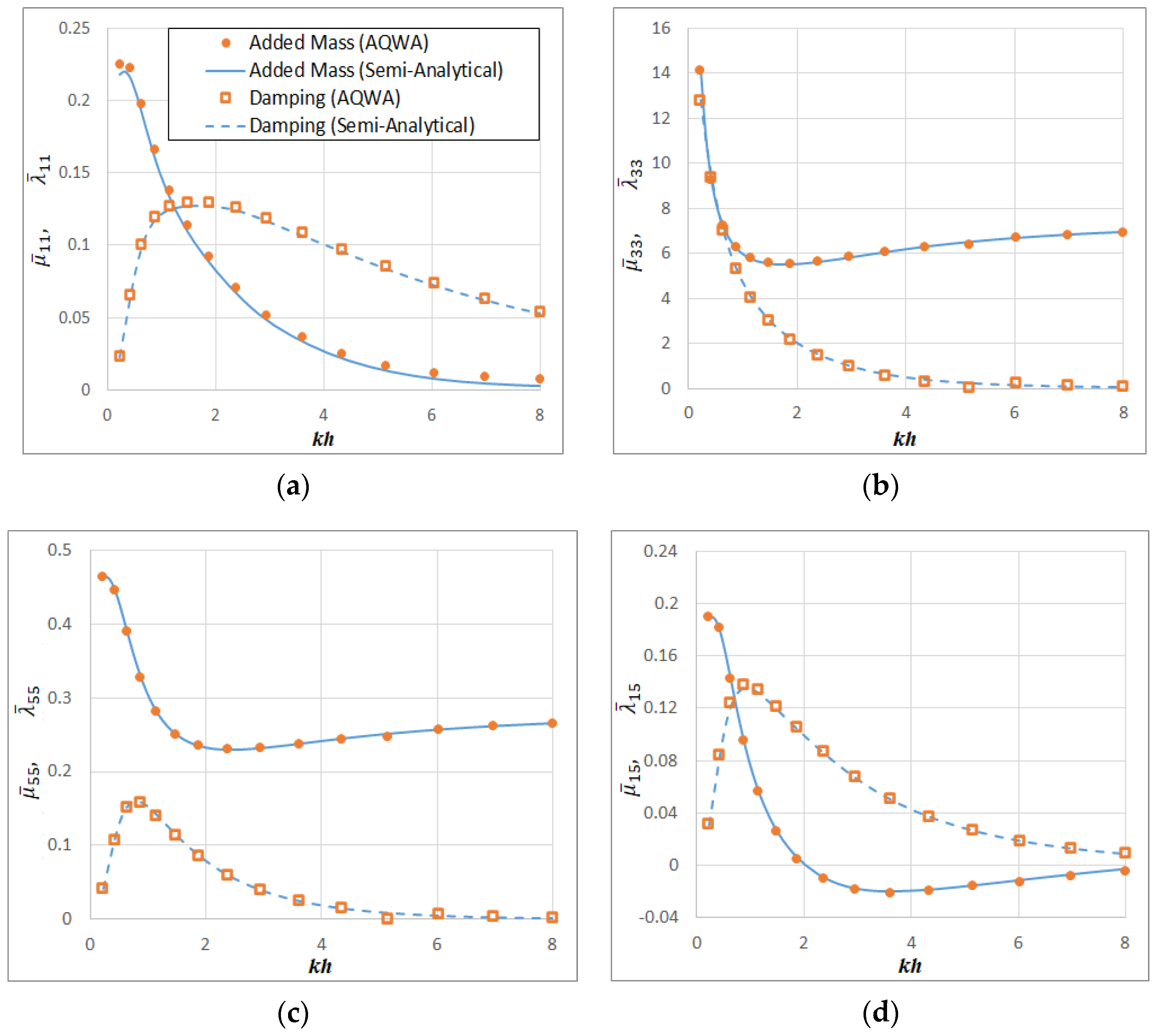
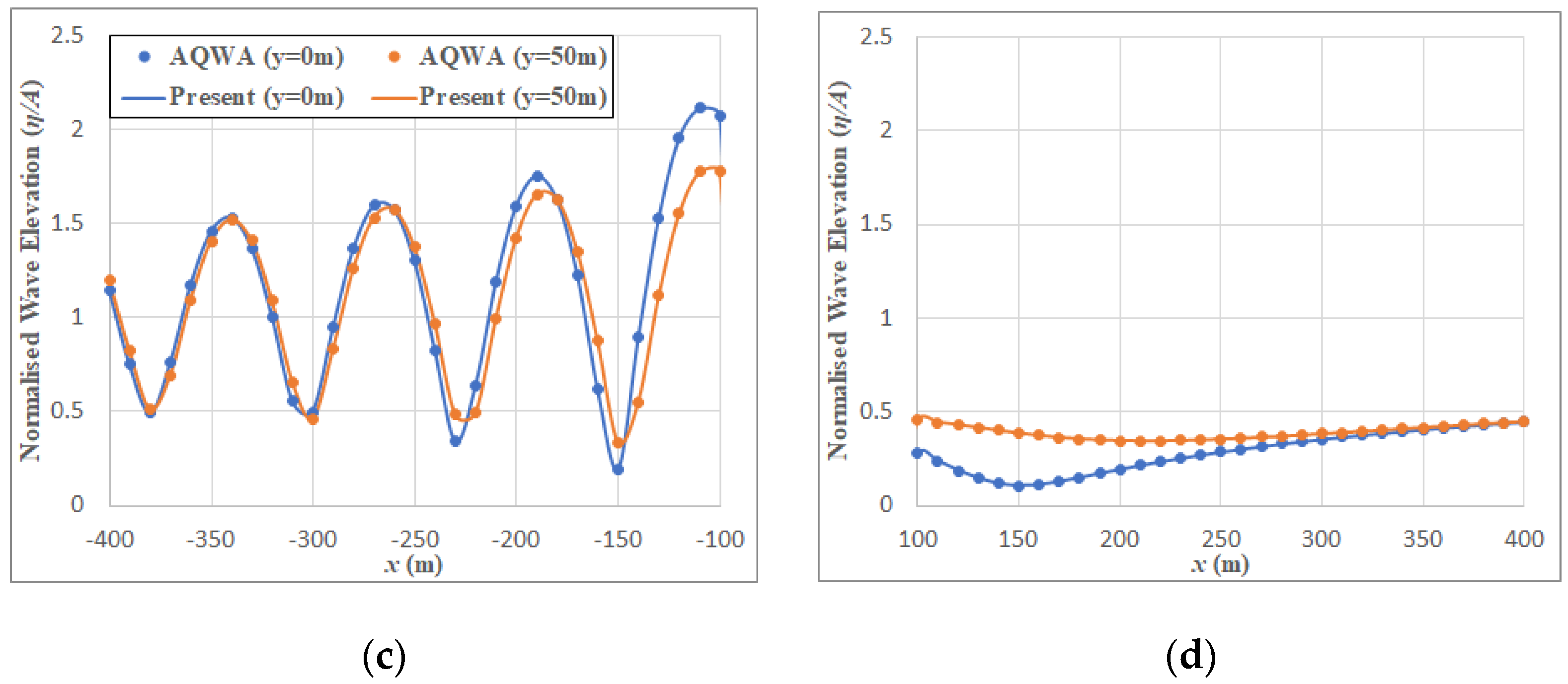
8. Verification of Semi-Analytical Approach and Computer Code

In order to verify the semi-analytical approaches and the computer code, we compare the hydrodynamic results (i.e., added mass, radiation damping, wave exciting forces, RAO, and wave field) with those obtained from the commercial software ANSYS AQWA based on the boundary element method.

For the verification exercise, we consider a floating hexagonal platform defined by radius function in Equation (1) with $R_0=100 \mathrm{m}$, $\epsilon =0.03$, $n_r=6$ and ${\theta }_0=\frac{\pi }{6}$ and the draft is 10 m. Figure 2 shows the platform shape. It is assumed that the centre of gravity coincides with the origin and the water depth is 50 m. The incident wave is along the x-axis (i.e., $\beta =0°)$.

For the 3D model in AQWA, the maximum mesh size is 2.6 m, which leads to a total of 17,087 diffracting elements to be used. The regular wave angular frequency domain is divided into 15 frequencies for the interval [0.1 rad/s, 1.2528 rad/s].

Figure 3a–d present the added mass and radiation damping obtained from present semi-analytical approaches and AQWA. The numbers of truncated terms for the hexagonal platform were conservatively taken as M = 18, N = 10, N_r = 6, Q = 12 for parametric studies. The two semi-analytical approaches provided the same results. The added masses were normalised by

$${\overline{\mu }}_{11}=\frac{{\mu }_{11}}{\rho S_{0}d}; {\overline{\mu }}_{33}=\frac{{\mu }_{33}}{\rho S_{0}d}; {\overline{\mu }}_{55}=\frac{{\mu }_{55}}{\rho S_0^{2}d}; {\overline{\mu }}_{15}=\frac{{\mu }_{15}}{\rho S_0^{1.5}d}$$

(83)

while the radiation damping was normalised by

$${\overline{\lambda }}_{11}=\frac{{\lambda }_{11}}{\rho \omega S_{0}d}; {\overline{\lambda }}_{33}=\frac{{\lambda }_{33}}{\rho \omega S_{0}d}; {\overline{\lambda }}_{55}=\frac{{\lambda }_{55}}{\rho \omega S_0^{2}d}; {\overline{\lambda }}_{15}=\frac{{\lambda }_{15}}{\rho \omega S_0^{1.5}d}$$

(84)

where $S_0$ is the cross-sectional area of the platform. The present semi-analytical results and AQWA results are in excellent agreement, thereby confirming the validity, convergence, and accuracy of the semi-analytical approaches.

In view of the cosine-type radius function, it is unnecessary to perform the integration for all the series terms, but series index m can be restricted to

$$\begin{gathered} m=\pm 1, \pm \left(n_r\pm 1\right) \mathrm{for} \mathrm{surge} \mathrm{or} \mathrm{sway} \\ m=0, \pm n_r \mathrm{for} \mathrm{heave} \\ m=0^{*},\pm 1, \pm \left(n_r\pm 1\right), \pm \left(2n_r\pm 1\right), \pm n_r{}^{*} \mathrm{for} \mathrm{roll} \mathrm{or} \mathrm{pitch} \\ m=0,\pm 1^{*},\pm 2,\pm n_r, \pm {\left(n_r\pm 1\right)}^{*}, \pm \left(n_r\pm 2\right),\pm \left(2n_r\pm 1\right), \pm 2n_r \mathrm{for} \mathrm{yaw} \end{gathered}$$

(85)

where $n_r$ is the parameter of the radius function given in Equation (1) and the superscript * denotes that it is only effective when $x_G$ or $y_G$ is nonzero. For example, if $n_r=6$ is taken for a hexagonal platform, one can choose $m=\pm 1$, $\pm 5$ and $\pm 7$ for surge. This rule can be equally applied for calculating the wave exciting forces.

The wave exciting forces and RAOs were calculated for $\beta =0°$. The surge force, heave force, and pitch moment were normalised as follows:

$$\overline{F_x}=\frac{F_x}{\rho gA{S}_0}; \overline{F_z}=\frac{F_z}{\rho gA{S}_0}; {\overline{M}}_y=\frac{M_y}{\rho gA{S}_{0}d}$$

(86)

The RAO (response amplitude operator) is defined as the motion response normalised by the incident wave amplitude A. Figure 4 compares the wave exciting forces and the RAOs obtained from the present semi-analytical approaches and those computed from ANSYS AQWA. It can be seen that the results are in close agreement, thereby verifying the present semi-analytical formulation and method of solution.

The wave field around the hexagonal platform was calculated for the sea domain size of $800 \mathrm{m}\times 800 \mathrm{m}$ for shorter waves (T = 5 s) and for longer waves (T = 10 s). Figure 5 and Figure 6 show the wave fields and the wave profiles along the x-axis at y = 0 m and y = 50 m, which are normalised by the incident wave amplitude for the wave periods 5 s and 10 s, respectively. It can be seen that the wave fields obtained from the present approach and AQWA were well matched. The wave field belonging to AQWA was extracted from a large amount of AQWA FLOW raw data by writing a computer code to process the raw data at selected points.

Samples of the computational times required by different methods such as AQWA, the quadruple Fourier expansions by [15], semi-analytical approach 1, and semi-analytical approach 2 are noted and compared with one another in

Table 2. Comparison of computational times of different methods. (Note: values in parentheses denote the truncated numbers of M, N, N_r, and Q; NA, not applicable; and Δ denotes the maximum mesh size.)

T (s)	AQWA	Fourier Expansion [15]	Semi-Analytical Approach 1	Semi-Analytical Approach 2
5	(Δ = 2.6 m)	(18, 5, 6, 12)	(18, 5, NA, NA)	(18, 5, 6, 12)
	8 min 18 s	26 s	48 s	16 s
10	(Δ = 10 m)	(10, 10, 6, 12)	(10, 10, NA, NA)	(10, 10, 6, 12)
	24 s	30 s	23 s	19 s

. The computation was conducted by using a personal computer with Intel(R) Core(TM) i7-7700 CPU @ 3.60 GHz and 16 GB RAM. Suitable truncation numbers $M$, $N$, $N_r$, and $Q$ were used for each case. The wave periods considered were $T=5 \mathrm{s} \mathrm{and} 10 \mathrm{s}$. The computational time of AQWA was obtained by checking the file created time in Windows Explorer. It can be seen that AQWA takes a significantly more computational time, when compared to the other three analytical methods, for determining the velocity potentials as the wave period becomes shorter. AQWA uses eight CPU cores and the computation runs in a console environment that enables the computation to be extremely fast, whereas the present semi-analytical approaches run on the MATLAB application platform with the default number of CPU cores. Of the three semi-analytical approaches, the semi-analytical approach 2 uses the least computational time, and hence this method is recommended for determining velocity potentials for floating platforms and for performing parametric studies.

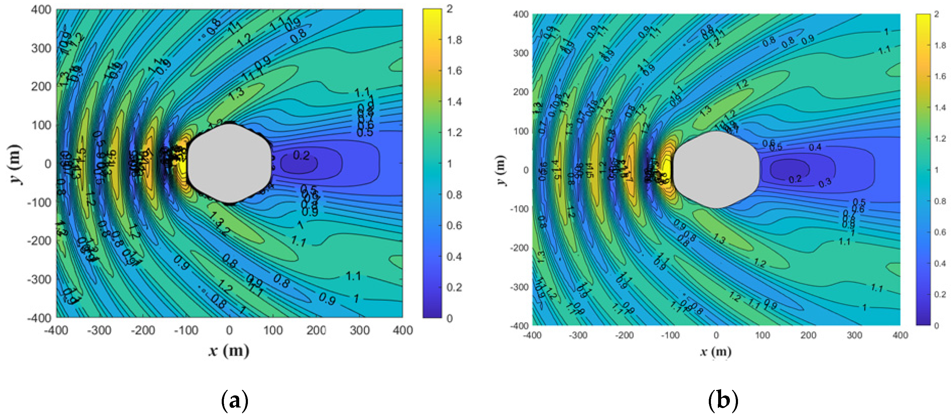
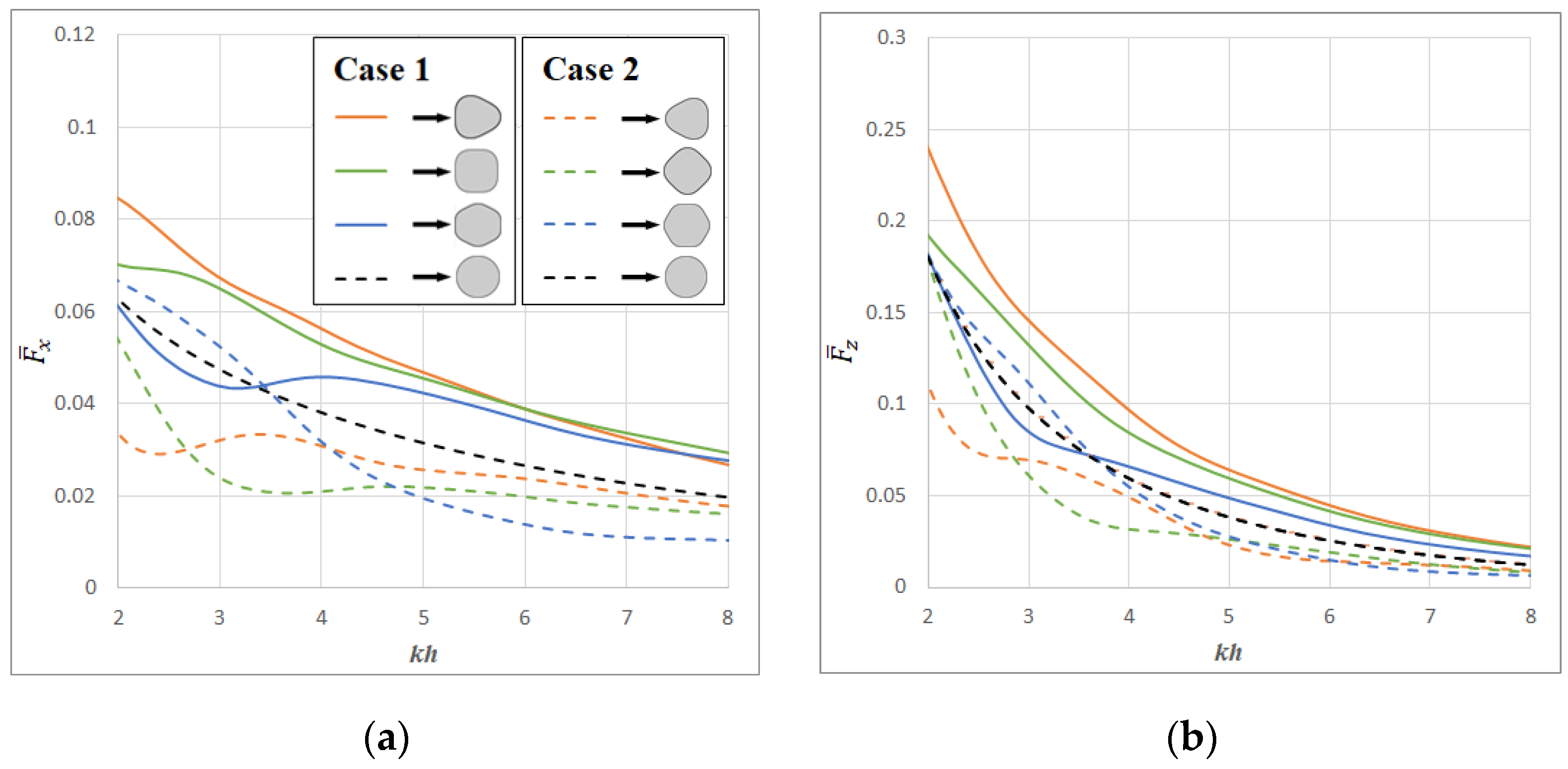
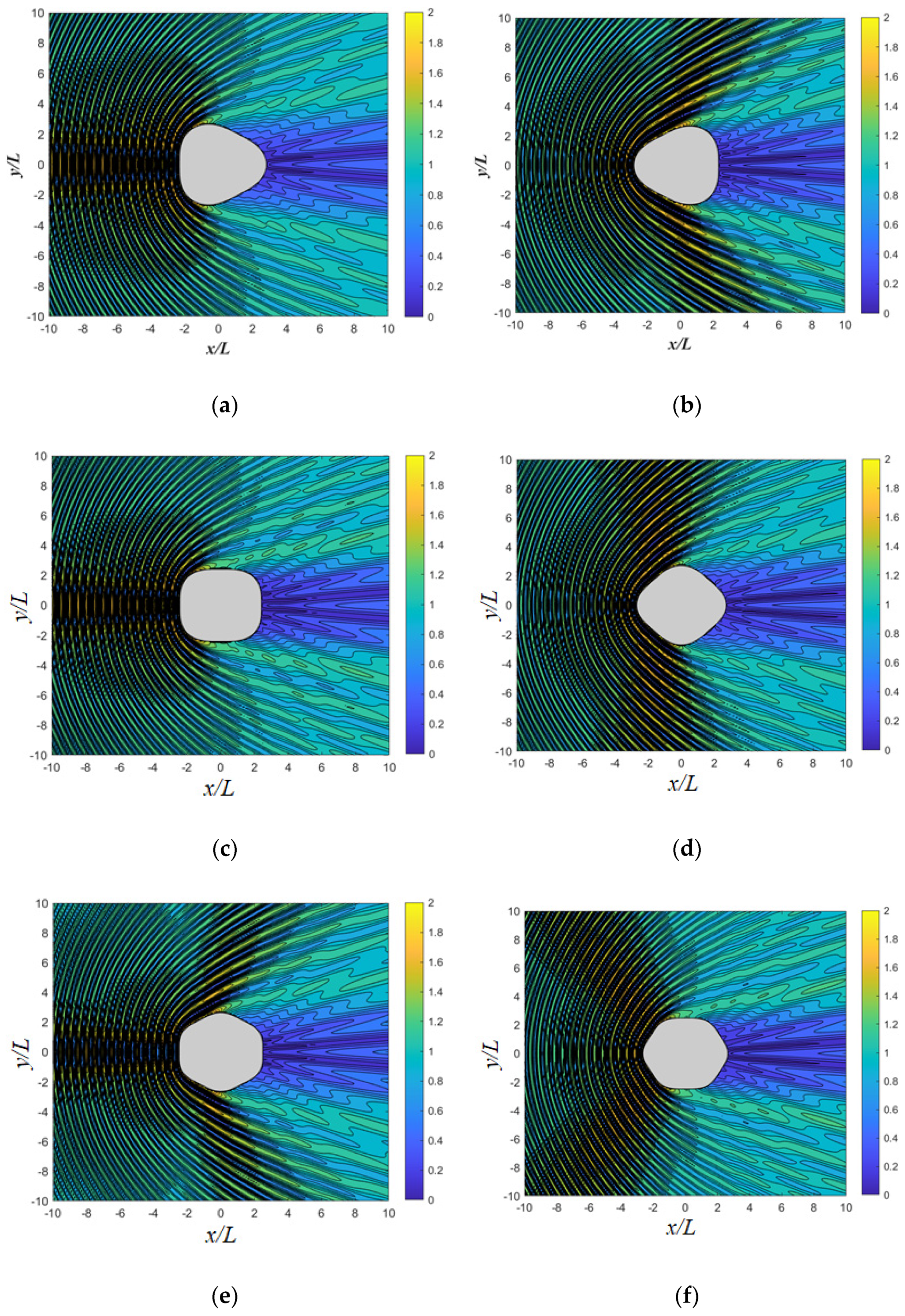
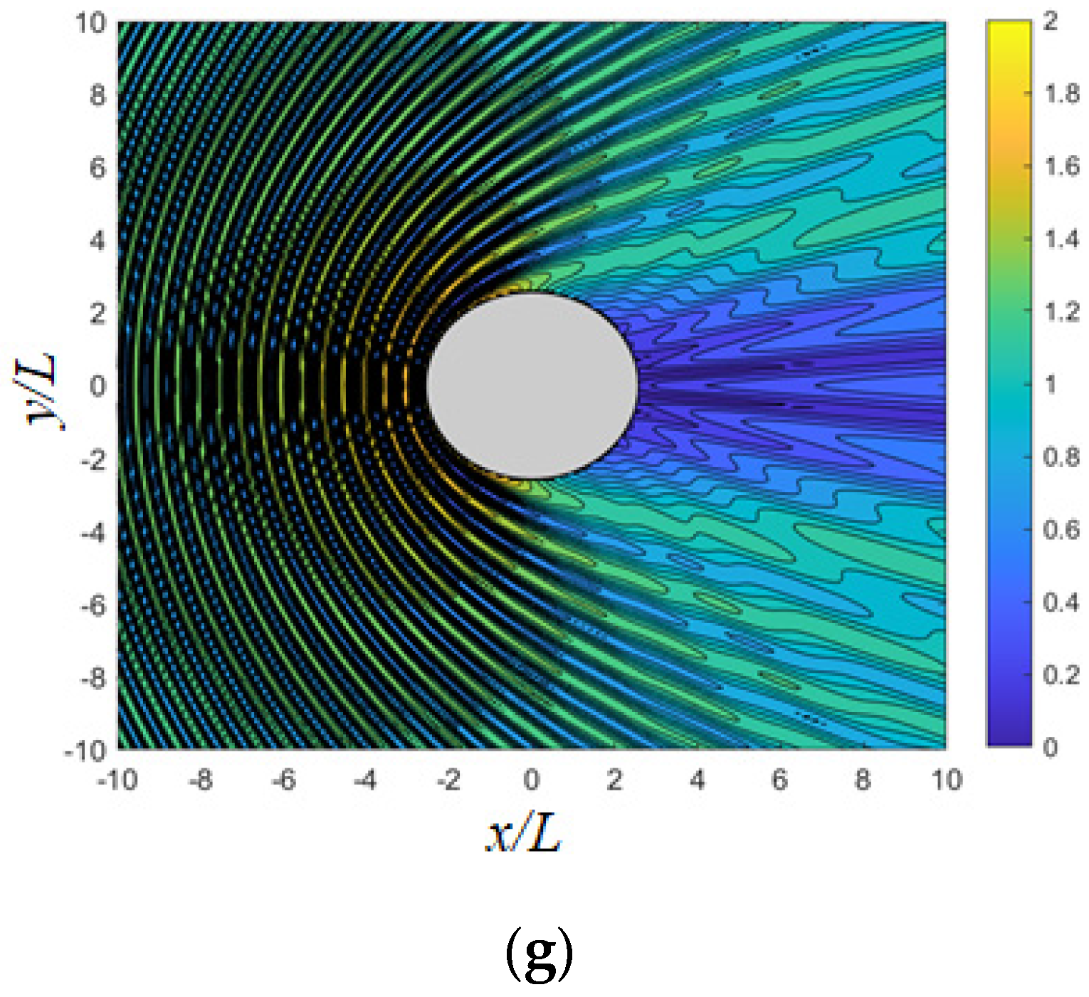
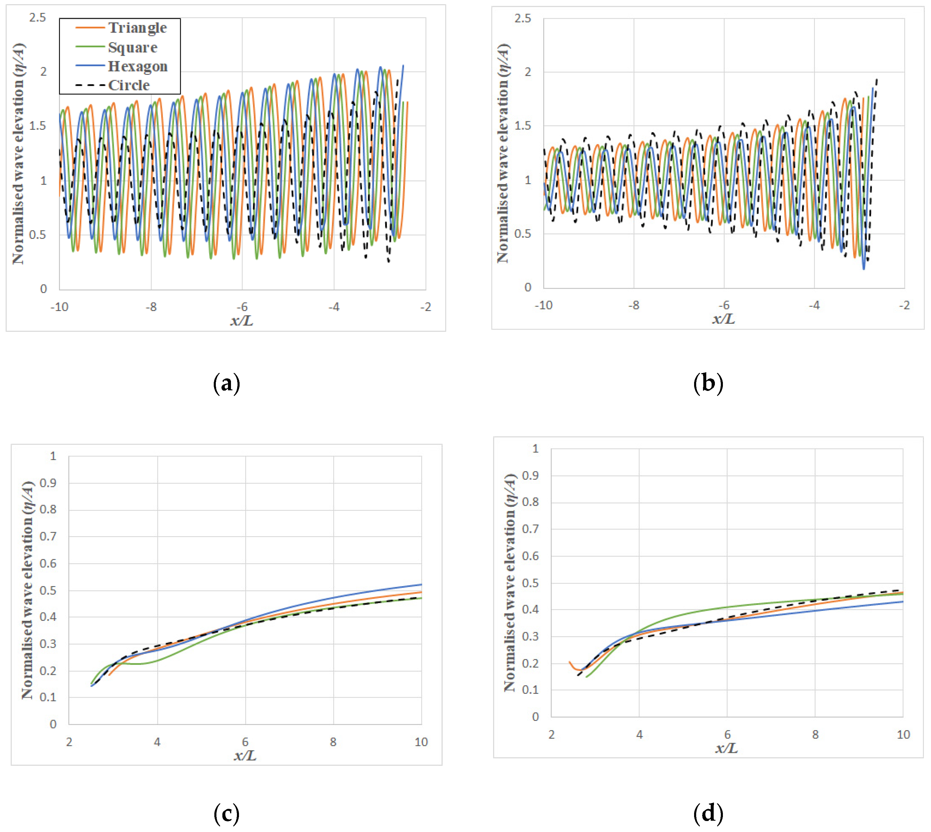
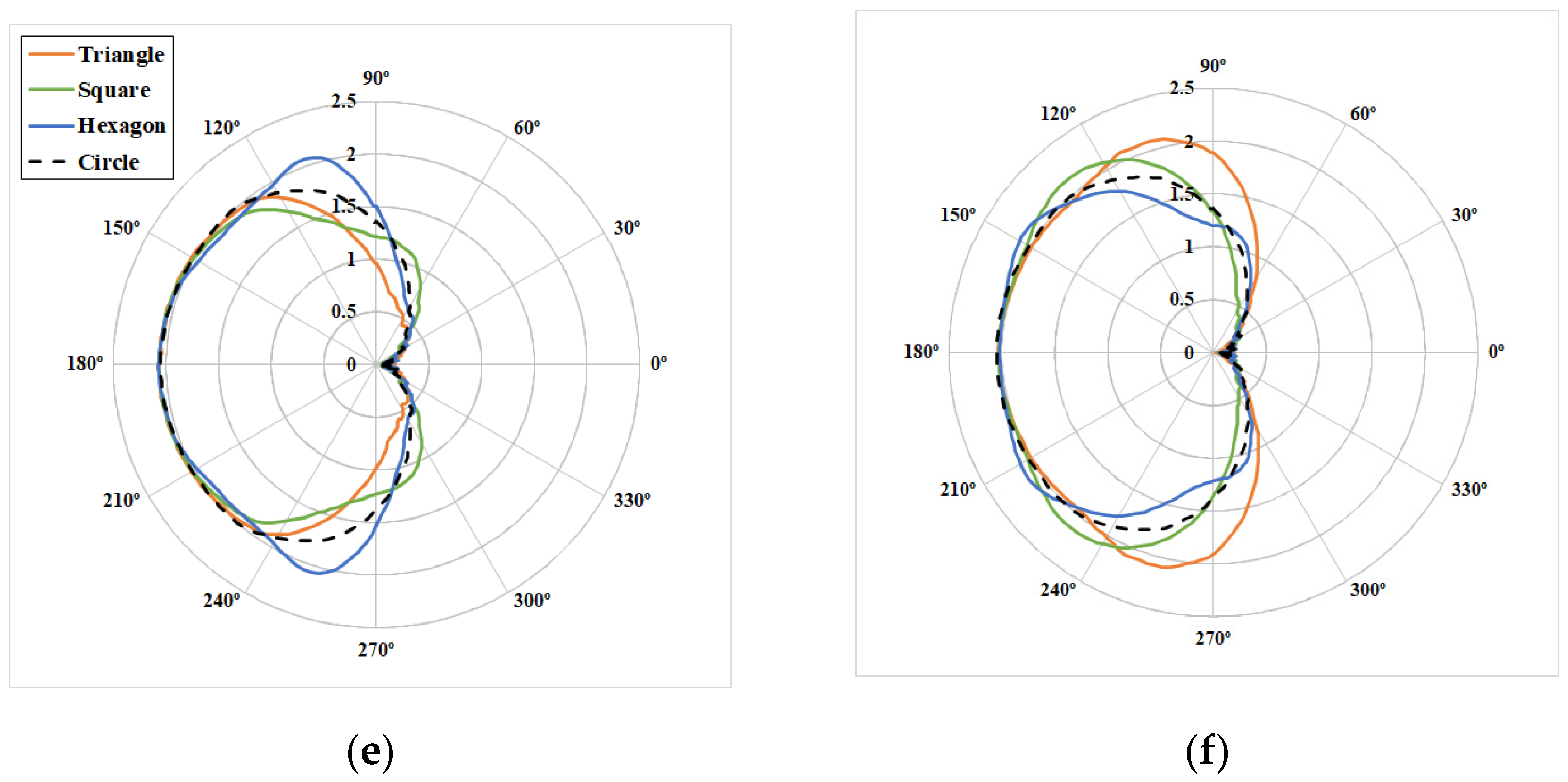
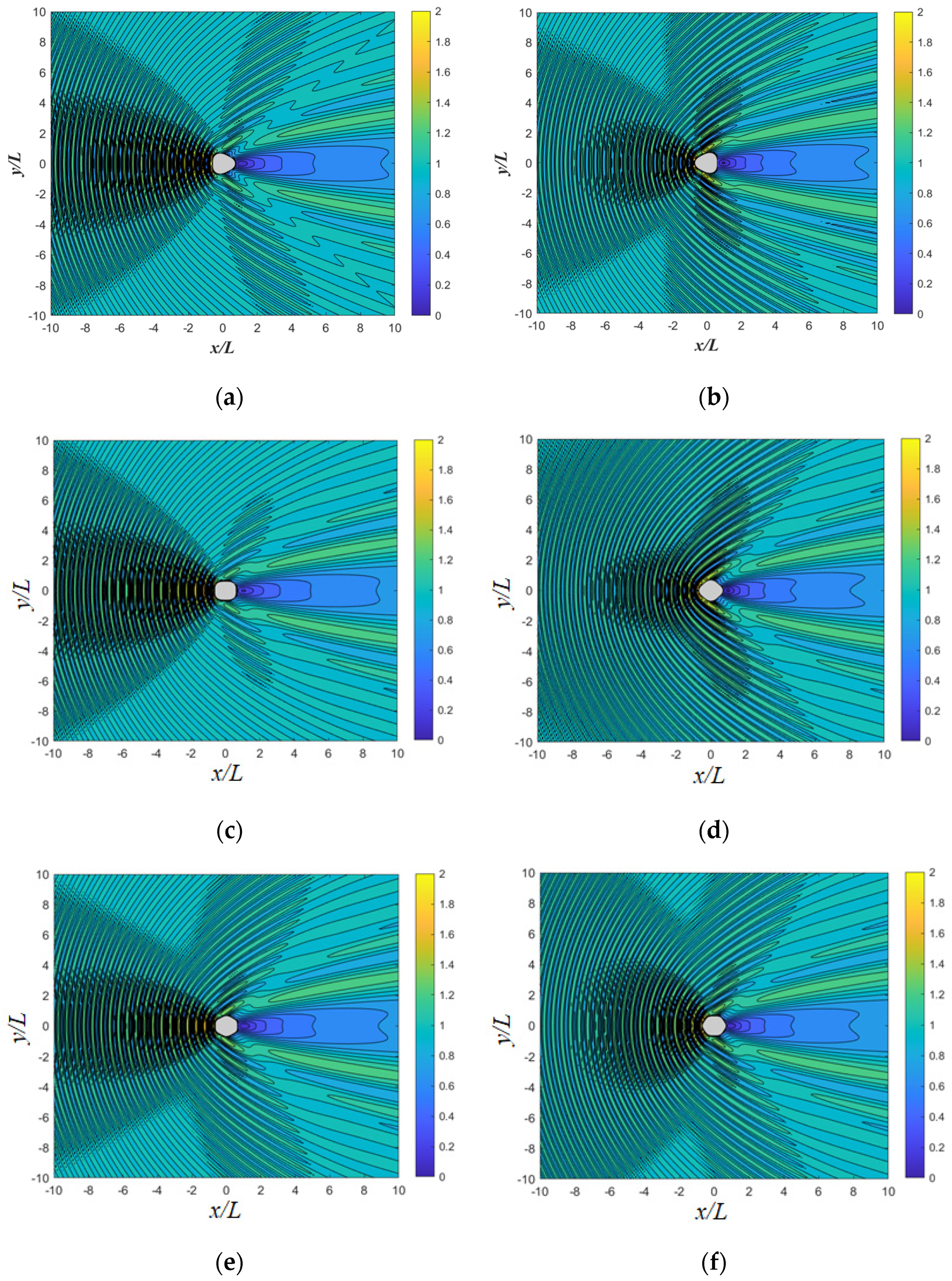
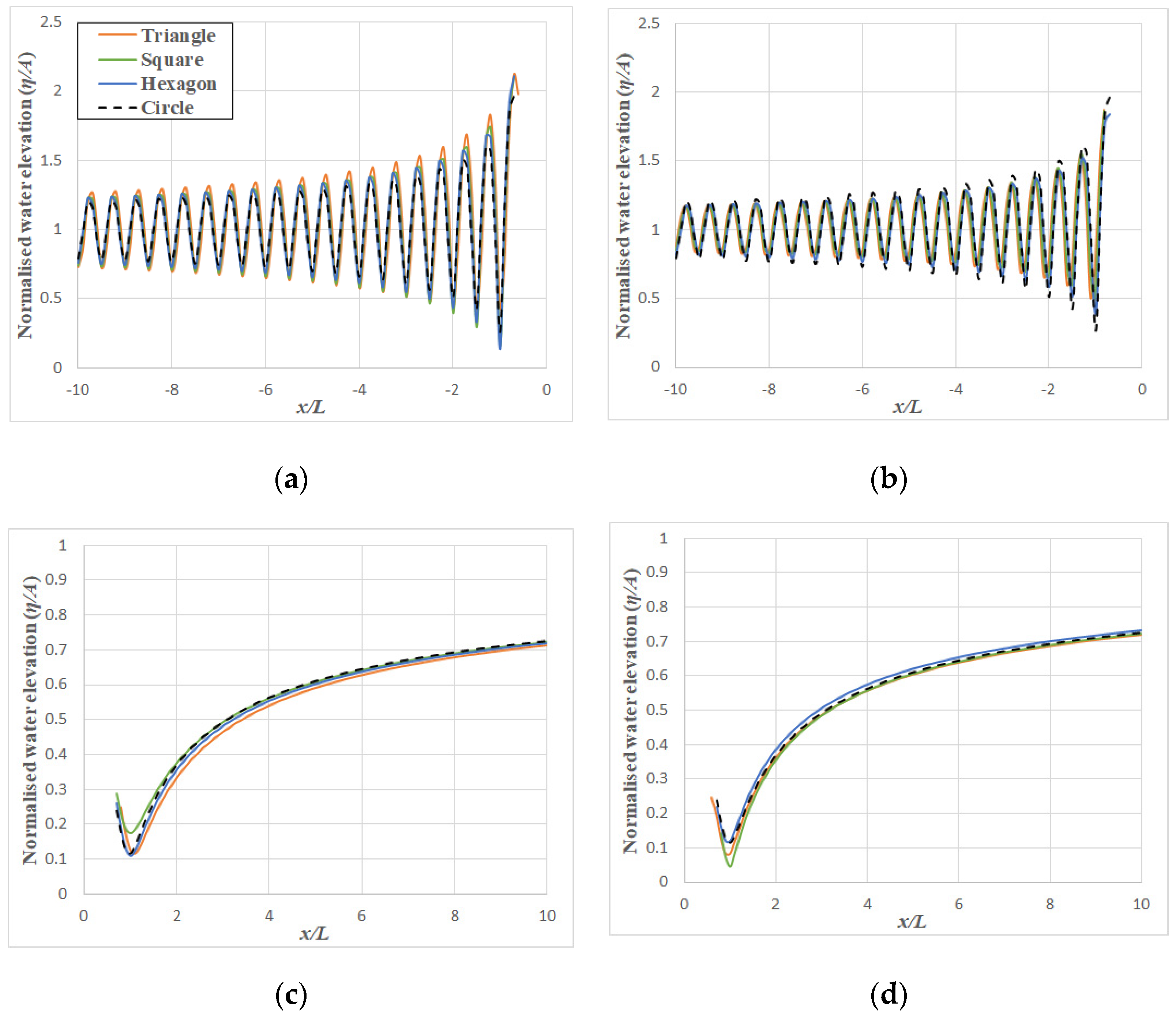
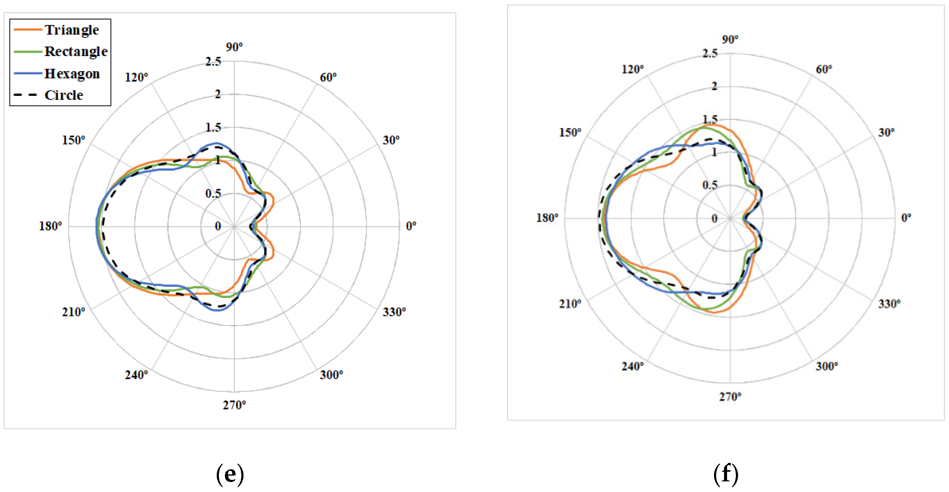
9. Hydrodynamic Results of Polygonal Platforms

Based on semi-analytical approach 2, one may obtain the hydrodynamic coefficients (added mass and radiation damping), wave exciting forces, RAOs, and wave fields for various platform shapes. In this section, we present results for triangular, square, hexagonal, and circular platforms. The platforms have almost the same plan area of $\pi R_0^2$. Consider a radius $R_0$ of 100 m, draft of 10 m, and water depth h = 50 m. We assume wave periods to range from 5 s to 10 s. Based on this wave period and the assumed water depth, relative wave number kh ranges from $2 \mathrm{to} 8$.

For the triangular, square, and hexagonal platforms, two cases were considered according to their orientation. For Case 1, the triangular platform was orientated 30° in the counter-clockwise direction based on Equation (1), but the square and hexagonal platforms were not orientated, while for Case 2, the triangular, square, and hexagonal platforms were respectively orientated 60, 45, and 30° from Case 1. The inset in Figure 7 shows the cases considered.

It was found that the added mass, radiation damping, and RAOs for the polygonal platforms considered were not distinctively different, and thus they are not presented. Figure 7 shows the variations of the surge, heave forces, and pitch moments on the platforms with respect to the relative wave number kh for Cases 1 and 2. For a given polygonal shaped platform, Case 2 curves are generally below Case 1 curves, which shows that the wave exciting forces and rotational moment can be reduced by orientating the polygonal platform with one of its corners in alignment with the wave incident direction. The reason may be explained by wave phase variations. When the incident wave is acting normal to the platform surface, the phase for the surge force is the same throughout that surface length, and thus the waves are amplified. However, when the waves impact on an inclined surface, the phase of the surge force varies along the length of the inclined surface, resulting in the reduction of the nett surge forces on the inclined surface of the platform. The results for the heave force and pitch moment behave in a similar manner. Case 1 curves are generally above the circular platform, with a downward trend with respect to increasing kh, whereas Case 2 curves are below the circular platform with irregular variations. This implies that polygonal platforms can have better hydrodynamic performance than the circular platform by appropriate orientation with respect to the prevailing wave direction (i.e., orientation of platform as in Case 2). The square platform with Case 2 orientation is hardly affected by the wave frequencies for the surge and heave forces when $kh\ge 3$. Similarly, for triangular platform with Case 1, the surge force is not significantly affected by a range of wave frequencies. It is clear that the circular platform is most suitable when there is no prevailing wave direction, i.e., the waves can approach from any direction.

Next, the wave fields around the different platforms were investigated for the wave periods $T=5 \mathrm{s} \mathrm{and} 10 \mathrm{s}$. Figure 8 represents the wave fields for $T=5 \mathrm{s}$. The coordinates x and y were normalised by the wavelength L. It can be seen that platforms for Case 1 are more likely to reflect the incident waves back to the incoming wave direction, while platforms for Case 2 are observed to redirect the incident waves to other directions such that the reflected waves for Case 2 are less amplified than Case 1. In the figure, the darker shades represent more wave crests and troughs. The circular platform is able to distribute the reflected waves in multiple directions, thus it creates relatively less reflected waves than the triangular, square, and hexagonal platforms with Case 1 orientation. This point is clearly seen by the wave profiles in the sea side at the centreline y = 0 m for $T=5 \mathrm{s}$ as presented in Figure 9a. Figure 9b shows that the polygonal platforms for Case 2, which reduce the wave amplitude in the sea side more than the circular platforms.

Generally, the considered polygonal platforms have slightly similar wave transmission performance as the circular platform as shown by the variation of the ratio of the transmitted wave elevation to the incident wave amplitude along the centreline y = 0 m for $T=5 \mathrm{s}$ (see Figure 9c,d). All platform shapes provide a reasonably large area of sheltered sea space (normalised wave elevation of less than 0.5 as far as 10 wave lengths or about 400 m from the centre of the platform).

Figure 9e,f shows the wave runups around the perimeter of platforms. It can be seen that the hexagonal platform for Case 1 has greater wave runup than the triangular and square platforms for Case 1. Thus the hexagonal platform for Case 1 will perform well for installation of wave energy converters for harvesting wave energy. For Case 2, however, the wave runup by the triangular platform is observed to be more pronounced than those by other platforms, and hence it will be a better platform shape for Case 2 for wave energy harvesting. It is clear that the best place for placing wave energy converters is where the wave runup is high. Many researchers ([20,21]) have studied the performance of wave energy converters placed in front of a breakwater. Moreover, the wave run-up information is useful in designing the freeboard to prevent wave overtopping.

The wave fields for $T=10 \mathrm{s}$ are shown in Figure 10. It can be clearly seen that Case 1 is more reflective than Case 2, whereas Case 2 is more dispersive than Case 1. In the dark shaded region, wave crests and troughs are concentrated and the areas of the darkest shades for Case 1 are larger than Case 2. The wave fields allow the designer to know how best to orientate the polygonal platform to reduce the reflected waves that may cause problems for ships or marine vessels passing by the platform. Regarding the reduction of reflected waves, it is clear that the polygonal platform should be orientated as in Case 2.

The corresponding wave profiles for T = 10 s are presented in Figure 11. It can be seen from Figure 11a,b that all platform shapes show coincidentally similar wave reflection profiles.

With regard to transmitted waves on the lee side of the platform, all polygonal platforms are able to provide a normalised transmitted wave elevation less than 0.5 for about three wavelengths (i.e., 450 m) from the centre of the platform (see Figure 11c,d).

Figure 11e,f shows the wave runups around the perimeter of platforms. It can be seen that the variations of the wave runups around the perimeter of all platform shapes are similar for long wave periods (e.g., T = 10 s). When compared to the figures for the shorter wave case, the enclosed area for the longer wave case is smaller. This implies wave energy harvesting will be more efficient for a shorter wave condition. Under a short-wave condition, wave overtopping may be more serious than under a long wave condition, depending on the platform’s wave transmission performance.

10. Conclusions

By using the proposed semi-analytical approach based on the eigenfunction expansion method, hydrodynamic performances of triangular, square, hexagonal, and circular platforms of similar size were investigated. The results show that these similar-sized platforms have similar added mass, radiation damping, and RAOs. However, the wave exciting forces and rotational moments differ for the different polygonal shapes. The surge force is observed to be reduced significantly when the polygonal platform is oriented such that one of its corners is in the direction of the incident wave angle (i.e., Case 2). The reason may be explained by wave phase variations. When the incident wave is acting normal to the platform surface, the phase for the surge force is the same throughout the surface length and thus, the waves are amplified. However, when the waves impact on an inclined surface, the phase of the surge force varies along the length of the inclined surface, resulting in the reduction of the nett surge forces on the inclined surface of the platform. This reduction in surge force due to platform orientation with respect to the prevailing wave direction is beneficial as it leads to a more cost-effective mooring system.

By observing the wave fields, platforms associated with Case 1 reflect more waves than Case 2 because platforms with Case 2 are better in dispersing the waves. Thus, platforms oriented according to Case 2 will reduce the wave amplitudes in the sea side, which in turn will lessen problems for ships or marine vessels passing by the platform on the weather side.

From the comparison study between different polygonal platforms, their wave attenuation performances are slightly similar. These platforms can provide a normalised wave amplitude in the lee side of less than 0.5 for about 400 m from the centre of the platform of radius 100 m. The sheltered area on the lee side of the platform may be used for berthing of ships and for other sea activities.

With regard to wave runups around the perimeter of platforms, it is clear that these runups are larger on the weather side than the lee side, which indicates that the freeboard must be designed to be larger on the weather side, accordingly, to avoid wave overtopping. Wave energy converters should be placed on the weather side of the platform. The hexagonal platform for Case 1 and triangular platform for Case 2 are found to have larger wave runups along their perimeters on the weather side for shorter wave period (e.g., T = 5 s), which make them better platform shapes for harvesting wave energy. For a long wave period (e.g., T = 10 s), the variations of wave runups among all the platform shapes are slightly similar.

The semi-analytical methods developed herein for hydrodynamic analysis of floating polygonal platforms have the following advantages. Semi-analytical approach 1 involves numerical integration to calculate the functional orthogonality, which is a part of the process of the eigenfunction expansion method. In view of an arbitrary radius function that describes the platform plan geometry, the integration cannot be performed analytically, but numerical integration must be resorted to. Its advantage lies in avoiding the need to establish the additional numbers of terms to be used for the Fourier expansion series when compared to semi-analytical approach 2. Semi-analytical approach 2 improves on Liu et al. [15] Fourier expansion series by reducing the number of Fourier coefficient sets from 10 to only 3 resulting in a significant reduction of computational time. Thus, solutions can be obtained faster by using this second approach.

References

1. Wang, C.M.; Wang, B.T. Large Floating Structures; Springer: Singapore, 2015; Volume 3. [Google Scholar]
2. Dai, J.; Wang, C.M.; Utsunomiya, T.; Duan, W.H. Review of recent research and developments on floating breakwaters. Ocean Eng. 2018, 158, 132–151. [Google Scholar] [CrossRef]
3. VisitSeoul. Sebitseom. Available online: https://english.visitseoul.net/nature/Sebitseom-en_/24646 (accessed on 25 July 2021).
4. Broom, D. Denmark Approves Artificial Island to Site 10 GW Offshore Win Hub. Available online: https://energypost.eu/denmark-approves-artificial-island-to-site-10gw-offshore-wind-hub/ (accessed on 25 July 2021).
5. Fishfarmexpert. FjordMAX Promises more Fish and Smaller Footprint. Available online: https://www.fishfarmingexpert.com/article/fjordmax-promises-more-fish-and-smaller-footprint/ (accessed on 25 July 2021).
6. Revkin, A. Floating Cities Could Ease the World’s Housing Crunch, the UN Says. Available online: https://www.nationalgeographic.com/environment/article/floating-cities-could-ease-global-housing-crunch-says-un (accessed on 25 July 2021).
7. Bai, K.J.; Yeung, R.W. Numerical solutions of free-surface flow problems. In Proceedings of the 10th Symposium Naval Hydrodynamics, Cambridge, MA, USA, 24–28 June 1974; pp. 609–641. [Google Scholar]
8. Mei, C.C. Numerical methods in water-wave diffraction and radiation. Annu. Rev. Fluid Mech. 1978, 10, 393–416. [Google Scholar] [CrossRef]
9. Garrison, C.J. Hydrodynamics of large objects in the sea, Part II: Motion of free-floating bodies. J. Hydronaut. 1975, 9, 58–63. [Google Scholar] [CrossRef]
10. Belibassakis, K. A boundary element method for the hydrodynamic analysis of floating bodies in variable bathymetry regions. Eng. Anal. Bound. Elem. 2008, 32, 796–810. [Google Scholar] [CrossRef]
11. Bhatta, D.; Rahman, M. On scattering and radiation problem for a cylinder in water of finite depth. Int. J. Eng. Sci. 2003, 41, 931–967. [Google Scholar] [CrossRef]
12. Yeung, R.W. Added mass and damping of a vertical cylinder in finite-depth waters. Appl. Ocean Res. 1981, 3, 119–133. [Google Scholar] [CrossRef]
13. Chen, H.S.; Mei, C.C. Scattering and Radiation of Gravity Waves by an Elliptical Cylinder, Report Number 140; Massachusetts Institute of Technology: Cambridge, MA, USA, 1971. [Google Scholar]
14. Williams, A.; Darwiche, M. Wave radiation by truncated elliptical cylinder. J. Waterw. Port Coast. Ocean Eng. 1990, 116, 101–119. [Google Scholar] [CrossRef]
15. Liu, J.; Guo, A.; Fang, Q.; Li, H.; Hu, H.; Liu, P. Investigation of linear wave action around a truncated cylinder with non-circular cross section. J. Mar. Sci. Technol. 2018, 23, 866–876. [Google Scholar] [CrossRef]
16. Yu, H.; Zheng, S.; Zhang, Y.; Iglesias, G. Wave radiation from a truncated cylinder of arbitrary cross section. Ocean Eng. 2019, 173, 519–530. [Google Scholar] [CrossRef]
17. Mansour, A.M.; Williams, A.N.; Wang, K. The diffraction of linear waves by a uniform vertical cylinder with cosine-type radial perturbations. Ocean Eng. 2002, 29, 239–259. [Google Scholar] [CrossRef]
18. Liu, J.; Guo, A.; Li, H. Analytical solution for the linear wave diffraction by a uniform vertical cylinder with an arbitrary smooth cross-section. Ocean Eng. 2016, 126, 163–175. [Google Scholar] [CrossRef]
19. Lee, C.H. WAMIT Theory Manual; Department of Ocean Engineering, Massachusetts Institute of Technology: Boston, MA, USA, 1995. [Google Scholar]
20. Mavrako, S.; Katsaounis, G.; Nielsen, K.; Lemonis, G. Numerical performance investigation of an array of heaving wave power converters in front of a vertical breakwater. In Proceedings of the Fourteenth International Offshore and Polar Engineering Conference, Toulon, France, 23–28 May 2004. [Google Scholar]
21. Konispoliatis, D.N.; Mavrakos, S.A. Theoretical performance investigation of a vertical cylindrical oscillating water column device in front of a vertical breakwater. J. Ocean Eng. Mar. Energy 2020, 6, 1–13. [Google Scholar] [CrossRef]
Figure 1. Floating polygonal platform under wave action.
Jmse 09 00923 g001
Figure 2. Hexagonal platform for verification study: (a) plan view; (b) 3D mesh model (AQWA).
Jmse 09 00923 g002
Figure 3. Comparison of added mass and radiation damping obtained from AQWA and semi-analytical method: (a) for μ ¯ 11 and λ ¯ 11 ; (b) for μ ¯ 33 and λ ¯ 33 ; (c) for μ ¯ 55 and λ ¯ 55 ; and (d) for μ ¯ 15 and λ ¯ 15 .
Jmse 09 00923 g003
Figure 4. Comparison of wave exciting forces and RAOs obtained from AQWA and semi-analytical approach: (a) surge force; (b) heave force; (c) pitch moment; (d) RAO for surge motion; (e) RAO for heave motion; and (f) RAO for pitch motion.
Jmse 09 00923 g004
Figure 5. Comparison of normalised wave elevations obtained from AQWA and semi-analytical approach (for T = 5 s): (a) wave field from semi-analytical approach; (b) wave field from AQWA; (c) wave profiles in the sea side; and (d) wave profiles in the lee side.
Jmse 09 00923 g005
Figure 6. Comparison of normalised wave elevations obtained from AQWA and semi-analytical approach (for T = 10 s): (a) wave field from semi-analytical approach; (b) wave field from AQWA; (c) wave profiles in the sea side; and (d) wave profiles in the lee side.
Jmse 09 00923 g006aJmse 09 00923 g006b
Figure 7. Comparison of wave exciting forces for different platform shapes: (a) surge force; (b) heave force; and (c) pitch moment.
Jmse 09 00923 g007aJmse 09 00923 g007b
Figure 8. Wave fields for triangular, square, hexagonal, and circular platforms (T = 5 s): (a) triangular platform (Case 1); (b) triangular platform (Case 2); (c) square platform (Case 1); (d) square platform (Case 2); (e) hexagonal platform (Case 1); (f) hexagonal platform (Case 2); and (g) circular platform.
Jmse 09 00923 g008aJmse 09 00923 g008b
Figure 9. Wave profiles for triangular, square, hexagonal, and circular platforms (T = 5 s): (a) wave profiles in the sea side for Case 1; (b) wave profiles in the sea side for Case 2; (c) wave profiles in the lee side for Case 1; (d) wave profiles in the lee side for Case 2; (e) wave runup for Case 1; and (f) wave runup for Case 2.
Jmse 09 00923 g009aJmse 09 00923 g009b
Figure 10. Wave fields for triangular, square, hexagonal, and circular platforms (T = 10 s): (a) triangular platform (Case 1); (b) triangular platform (Case 2); (c) square platform (Case 1); (d) square platform (Case 2); (e) hexagonal platform (Case 1); (f) hexagonal platform (Case 2); and (g) circular platform.
Jmse 09 00923 g010aJmse 09 00923 g010b
Figure 11. Wave profiles for triangular, square, hexagonal, and circular platforms (T = 10 s): (a) wave profiles in the sea side for Case 1; (b) wave profiles in the sea side for Case 2; (c) wave profiles in the lee side for Case 1; (d) wave profiles in the lee side for Case 2; (e) wave runup for Case 1; and (f) wave runup for Case 2.
Jmse 09 00923 g011aJmse 09 00923 g011b