Article

Characteristics of Three-Dimensional Sound Propagation in Western North Pacific Fronts

1
Acoustic Science and Technology Laboratory, Harbin Engineering University, Harbin 150001, China
2
Key Laboratory of Marine Information Acquisition and Security, Ministry of Industry and Information Technology, Harbin Engineering University, Harbin 150001, China
3
College of Underwater Acoustic Engineering, Harbin Engineering University, Harbin 150001, China
*
Author to whom correspondence should be addressed.
J. Mar. Sci. Eng. 2021, 9(9), 1035; https://doi.org/10.3390/jmse9091035
Submission received: 30 August 2021 / Revised: 15 September 2021 / Accepted: 16 September 2021 / Published: 19 September 2021
(This article belongs to the Special Issue Sea Level Fluctuations)

Abstract

:
Oceanic fronts involved by ocean currents led to strong gradients of temperature, density and salinity, which have significant effects on underwater sound propagation. This paper focuses on the impact of the oceanic front on three-dimensional underwater sound propagation. A joint experiment of ocean acoustic and physical oceanography at the western North Pacific fronts is introduced. The measurement data for sound waves passed through the oceanic front is processed. The results are analysed and compared with the numerical simulation. It was found that transmission loss presented some difference when the source was located in the front centre and sound waves propagated towards water mass on opposite sides of the front centre. And when the sound field is excited by the underwater explosion at a depth of 200 m, the effects of the horizontal refraction cannot be neglected. On the other hand, the transmission loss for sound pressure fell sharply and rose rapidly at the side of cold water masses.

1. Introduction

Mesoscale oceanic eddies and fronts, as complex ocean dynamic phenomenon, are energetic contributors to mixing. The oceanic fronts are the boundary between warm and cold water masses, with very significant differences in temperature, density and salinity [1]. There are different kinds of oceanic fronts, such as the large-scale meandering front, buoyancy forced coastal water mass fronts and the interface region between the deep-ocean and the coastal regions [2]. Fronts of Kuroshio is a type of oceanic front caused by intensified current led to a strong gradient of sound in the water column, which show a notable effect on sound propagation. The dynamic ocean sound speed leads to the change of long-range acoustic propagation travel time, the movement of the sound channel axis or/and convergence zone and the horizontal refraction of rays path [3,4].
Oceanic fronts are observed in the global ocean, such as the Antarctic gyre, the Gulf of Mexico, the region between Hawaii and Alaska and the Kuroshio extension area. Lots of work has been done in different parts of the ocean and indeed, one of the topics on the research of the front is the mechanism of the formation and extinction of the front. To survey the generation and to evaluate vertical motions of the near-surface front, Mahadevan analysed model simulations of the oceanic front [5]. Sokolov et al. [6] used the expendable bathythermograph (XBT) and satellite altimeter to identify the subtropical front near Antarctica and South Australia. The analysis of the front position helps to obtain variation information in the annual sea surface temperature. In the long-term observation of the temperature gradient of fronts in the western North Pacific, Levine et al. [7] summarised the influence of front on topography at different frontal zones. Yang et al. [8] generalized heat and energy transfer of fronts near the continental shelf in the South China Sea, especially the mass exchange and energy distribution in the vertical direction. The other research topic is the seasonal variation in front. Nakamura et al. [9] identified the reasons for the seasonal variations in salinity of the oceanic front in the vertical mixing layer of the western North Pacific. Nakamura proved that this variation in winter is mainly caused by strong eddies and deep-ocean cyclonic. Also, the mixing layer energy enhances in the middle of oceanic fronts, due to the existence of near-inertial internal waves in winter. The westward movement of frontal current affected by the invasion of the Kuroshio in the Luzon Strait is analyzed by Liu et al. [10]. The generation of temperature fronts was observed in summer, using the satellite remote sensing processed data. Xie et al. [11] outline that the season has no evident impact on the horizontal position of the front while the vertical structure in the Southwest Pacific. By measurement and statistics, they also concluded that the depth of the oceanic fronts in the subtropical zone in winter was greater than that in summer. The oceanic fronts on the continental shelf are observed by Tan et al. [12] in both spring and summer. Also, they modelled the three-dimensional current field of the oceanic fronts and obtained its dynamic mechanism and formation reason.
The horizontal asymmetry character resulted in the complication of acoustic propagation in the area of frequently occurs current. Therefore, many studies and researches have been done on sound wave propagation through fronts. Seismic waves reflection has been observed at the boundary between two water masses with different thermodynamic characteristics. Nakamura et al. [13] analysed the multi-channel seismic exploring data, inversed sound speed of the horizontal variation of the temperature front. It showed sound wave is blocked by variations of horizontal temperature using mathematically sound propagation models. Neubert et al. [14] choose acoustic rays theory to deduce the average coherence intensity of sound wave multiple paths caused by random oceanic front. Tang et al. [12] also discussed the sound propagation characteristics responses to the intensity variability of oceanic front in the South China Sea. Acoustic shadow zones are formed when the sound waves pass through the warm side of the oceanic front. Liu et al. [15] made a preliminary summary of sound propagation of acoustic pressure resulted from typical mesoscale phenomena, using the parabolic model FOR3D [16] to simulate the impact of mesoscale eddies and oceanic fronts on the sea surface acoustic channel and converging zone. In the Yellow sea, coupled normal mode theory used as a numerical method for traveltime tomography, estimated the subsurface velocity structure and inversed the thermocline significant changes caused by current quantitatively [17]. Due to the limitation of experimental conditions, they study sound propagation without considering sound wave horizontal refraction. The three-dimensional thermocline inversion remains to be further explored. Jian et al. [18] provided the difference of propagation loss of acoustic pressure with and without oceanic front by parabolic method. Guo et al. [19] studied the travel time of sound waves and distribution of sound pressure in the ocean of Taiwan.
Furthermore, researchers have paid extensive attention to Kuroshio fronts and perform a big amount of numerical and experimental studies. Chen et al. [20] applied the ray theory to simulate the sound propagation process of front and found a remarkable change of sound propagation at the surface sound channel [21]. Rainville et al. [22] explained the gradient of temperature arouse the signal variety in the East China Sea and verified by joint experiment processed data in 2001. Shapiro investigated propagating characteristics along with different directions of oceanic front in different seasons of the same year.
Although scientists have carried out a relatively comprehensive study on the western North Pacific front by comparing of oceanic fronts exists or not and obtained certain conclusions in the aspects of sound pressure transmission loss and time arrival structure, there is a lack of discussion and analysis on the three-dimensional sound field of the front. This paper discusses the degree of sound wave horizontal deflection with several depths of source and receiver and reveals strong horizontal refraction because of the oceanic front, moreover explains the anomalous distribution of the acoustic field, which is helping to design vertical spacing in an array and positions of the acoustic stations of acoustic tomography. This paper analyses numerically and experimentally how oceanic fronts affect three-dimensional acoustic propagation in the western North Pacific. As follows in Section 2, a three-dimensional oceanic front environment was modelled and used to resolve the sound propagation and the forecasting process of the sound transmission based on the ray theory. And then, the sound propagation experiments in the Kuroshio is introduced, and the comparison between the measured results and numerical results are carried out in Section 3. In Section 4, the numerical results of the three-dimension acoustic propagation and the horizontal refraction process are described, while conclusions and discussions are drawn in Section 5.

2. Numerical Analysis of Sound Propagation

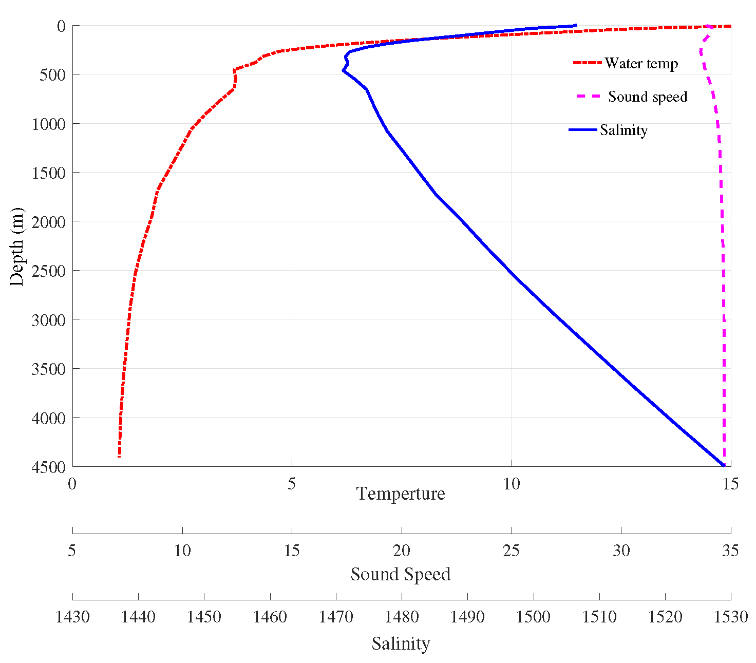
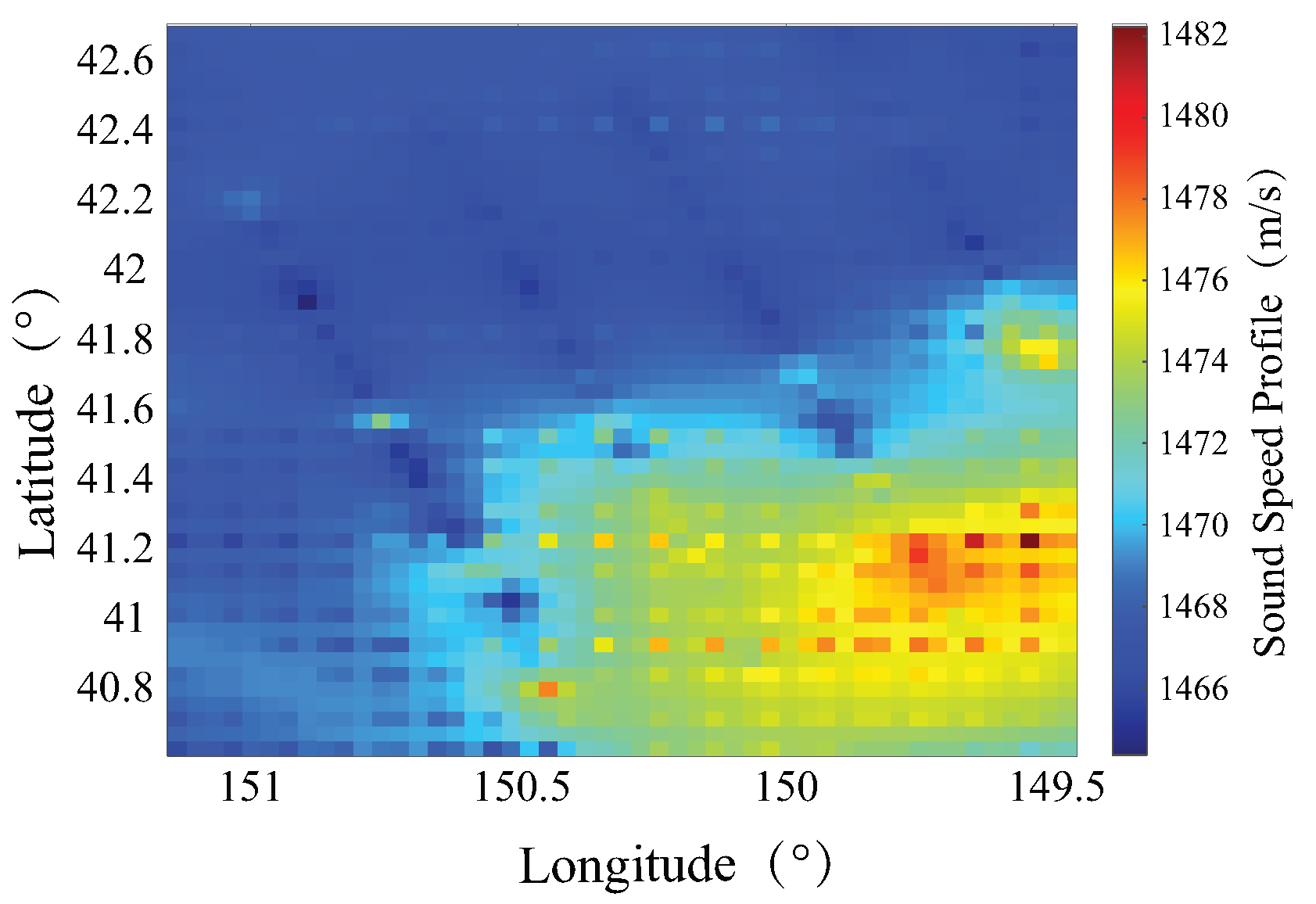
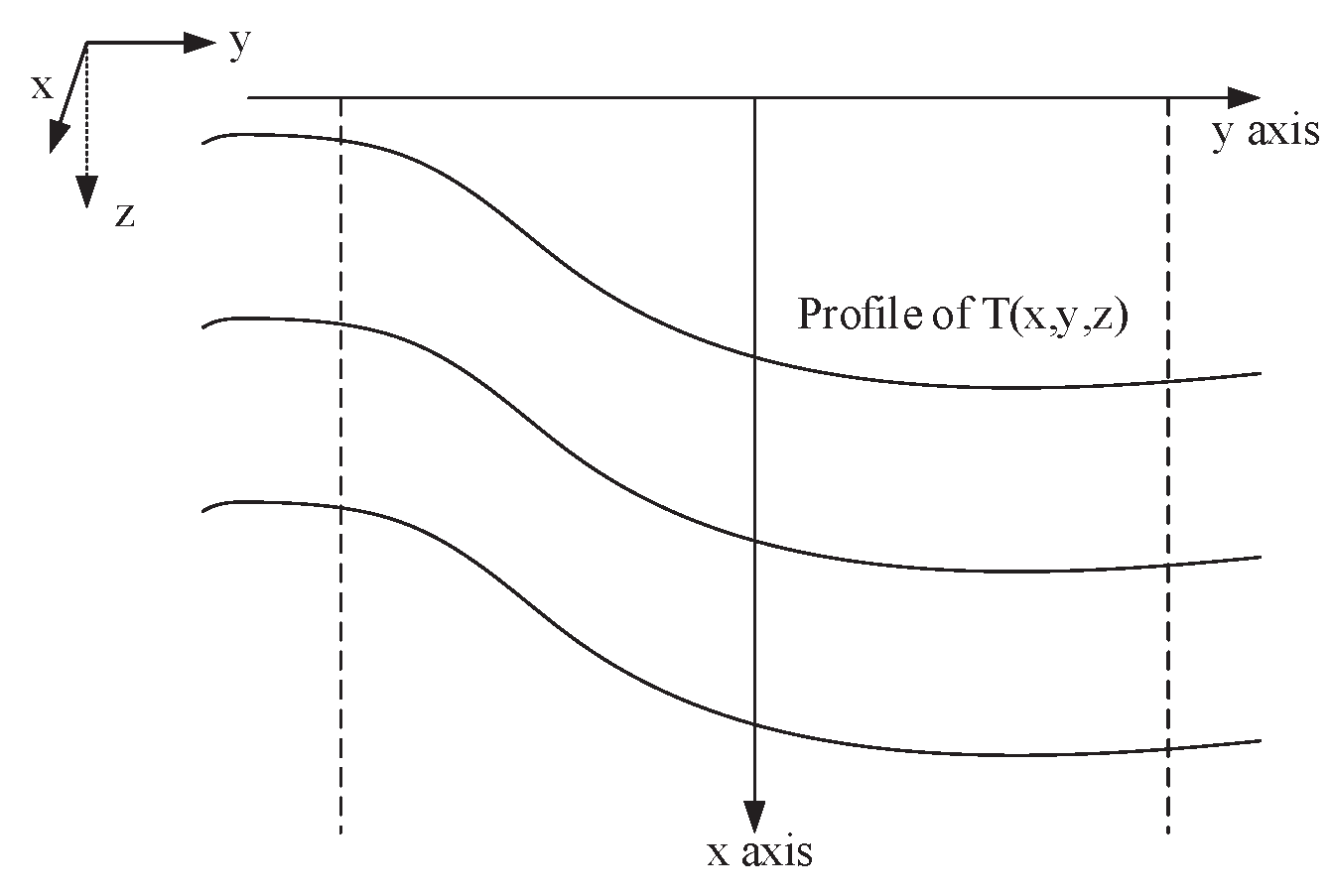
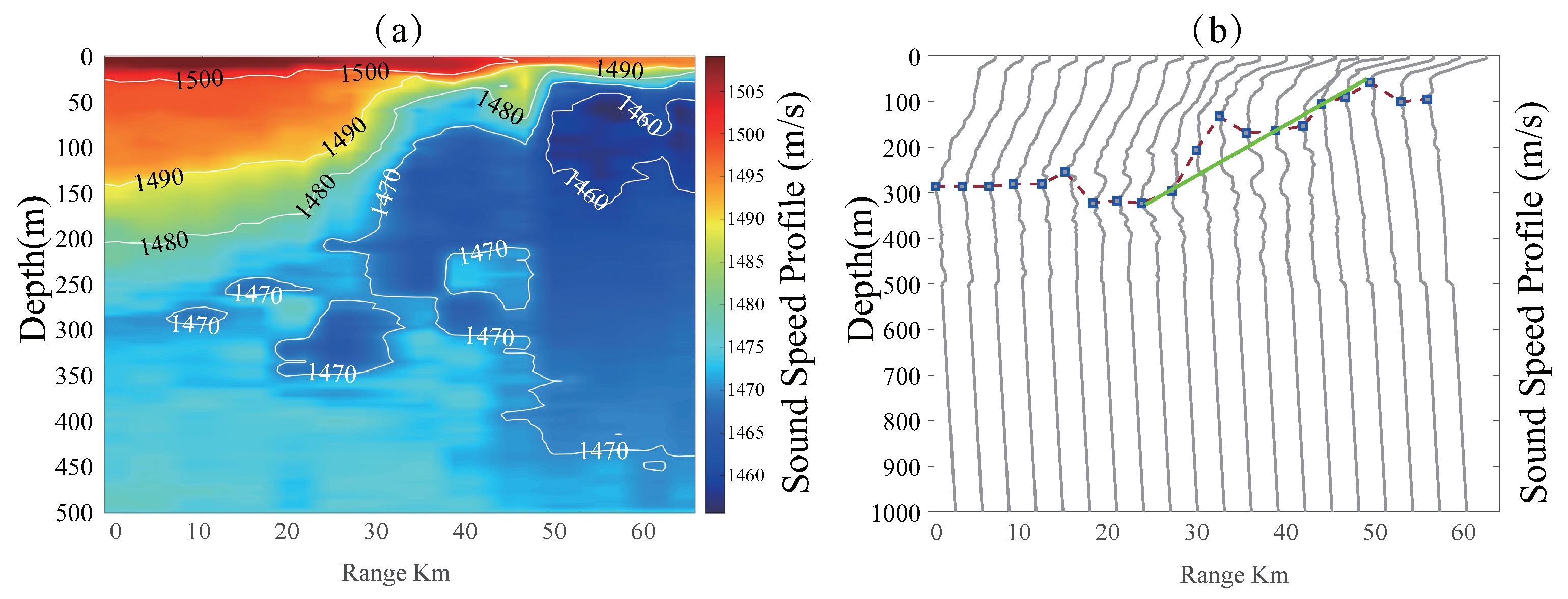
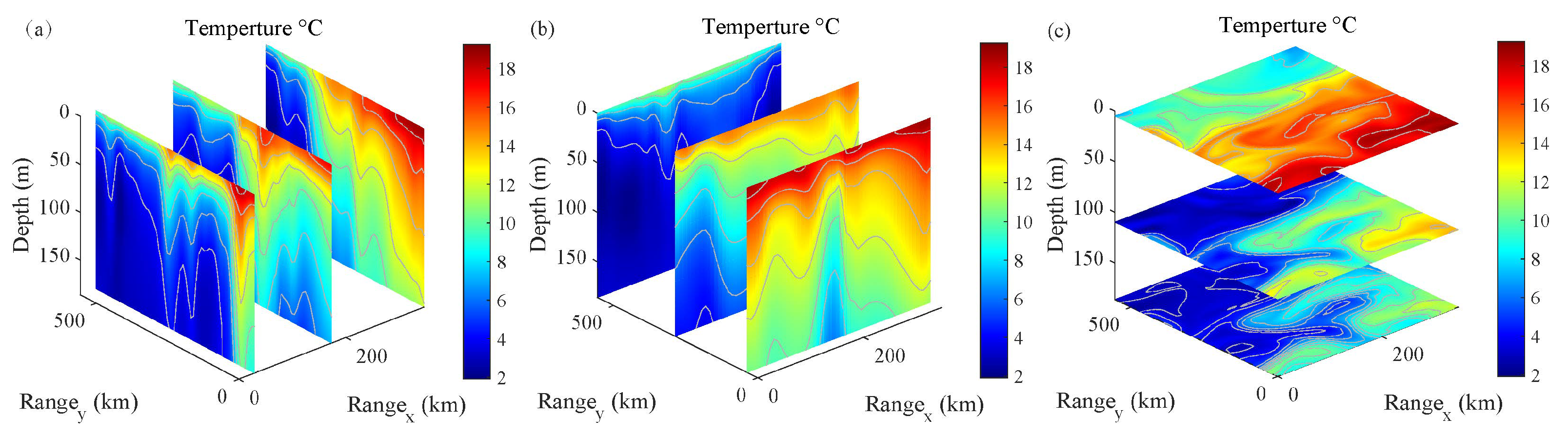
2.1. Distribution Model of Frontal Temperature and Salinity

The distribution of temperature and salinity of the oceanic front is presented based on their formation mechanism. Calado et al. [23] studied the characteristics of historical statistical data of oceanic front. Therefore the temperature characteristic equation of a large-scale front as follows Equation (1).
T ( x , y , z ) = [ T 0 ( x ) T b ( x ) ] Φ ( x , z ) + T b + α ( x , z ) Γ ( y )
where
  • T 0 ( x ) —surface temperature;
  • T b ( x ) —bottom temperature;
  • Φ ( x , z ) —non-dimensional temperature profile;
  • α ( x , z ) —along-steam distribution of the cross-frontal slope of the temperature;
  • Γ ( y ) —cross-frontal distribution of the temperature gradient α ( x , z ) .
Water fronts temperature feature model parameters are given in Figure 1, and the same equation and drawing can be used to describe the salinity distribution of the oceanic front. In the actual measurement process, the depths and positions of measured temperature and salinity data can not accommodate our needs regarding sound field simulation. In order to obtain a more accurate environmental distribution in the frontal area, the most frequently used method is spatial interpolation using limited field measurements and remotely sensed data. Considering the difference in the distance between the sampling location and the interpolation point, the interpolation method of inverse distance weighted should be adopted for temperature and salinity data based on the interpolation formula as Equation (2), where expression of T is temperatures or salinity vary with longitude and latitude.
T ( x , y ) = i = 1 N w i T ( x i , y i ) i = 1 N w i , where w i = 1 d ( x , y ; x i , y i ) 2
where
  • ( x , y ) —coordinates of observation point;
  • ( x i , y i ) —coordinates of interpolated point;
  • d—distance from ( x i , y i ) to ( x , y ) ;
  • N—total number of observation points used in interpolation.
To obtain the three-dimensional speed field around the oceanic front, and precise the distribution of vertical structure for the temperature, salinity and sound speed effectively, the extrapolation depth of the environmental data should be executed until the mean depths between the ocean surface and the sediment of this area (nearly 5 km). Alan B. Coppen’s [24] empirical formula as Equation (3) gives the relationship between the sound speed, temperature, salinity, and depth. Moreover, the limitation of temperature is 0 to 35 C and for salinity is 0 to 45 parts per thousand. Then it is easy to calculate the sound speed profile for this frontal area.
c ( x , y , z ) = c ( x , y , 0 ) + ( 16.23 + 0.253 t ) z + ( 0.213 0.1 t ) z 2 + [ 0.016 + 0.0002 ( S 35 ) ] ( S 35 ) t z , where c ( x , y , 0 ) = 1449.05 + 45.7 t 5.21 t 2 + 0.23 t 3 + ( 1.333 0.126 t + 0.009 t 2 ) ( S 35 )
where
  • t—temperature variable t = T ( x , y ) / 10 ;
  • T ( x , y ) —interpolated temperature in degrees Celsius;
  • S ( x , y ) —interpolated salinity in parts per thousand;
  • z—depth in kilometres.

2.2. Sound Propagation Model

With the rapid development of underwater acoustics since the 1980s, the commonly used numerical methods include normal mode theory, ray theory, parabolic equation theory and finite-element modelling [25]. Among them, normal mode theory solves the Sturm–Liouville eigenvalue problem of the acoustic wave; parabolic equation theory and finite-element theory as numerical methods could accurately solve the three-dimensional underwater acoustic problem. Both the parabolic equation theory and the ray theory are effective methods for predicting underwater sound propagation to solve the range-dependent ocean [26], however parabolic equation theory reduce timeliness and intuitiveness compared with ray theory. Ray tracking theory is based on the generalized Snell’s law [27], which adapts to study the sound deflection caused by the continuous variation of sound speed. Due to the different propagation paths of the acoustic ray from the source to the receiver position, the sound field at the receiving point is the superposition of the intensity of the ray path arrivals. The information including of each ray includes incident angle, soundtrack, intensity and phase. The horizontal deflection of the ray can be observed and verified intuitively by using the ray theory [28].
2 p ( X ) + ω 2 c 2 ( X ) p ( X ) = δ ( X X 0 )
where
  • ω —angular frequency of source signal;
  • X—receiver position;
  • X 0 —source position;
  • z—depth in kilometres.
Starting from the Helmholtz Equation (4), the sound pressure at a receiving position is actually a superposition of different acoustic rays (each ray is a normal to a wavefront), which can be expressed as,
p ( X ) = e i ω τ ( X ) j = 1 A j ( i ω ) j ( j = 1 , 2 , . . . ) , where τ ( s ) = τ ( 0 ) + 0 s c ( s ) d s
where
  • X—ray trajectory X = ( x , y , z ) ;
  • τ —travel times of the acoustic rays;
  • j—number of acoustic rays;
  • A j —amplitude of j th acoustic ray;
  • s—arclength along the ray;
  • s —ray trajectory;
  • c—sound speed at the position X.
Putting Equation (5) into Equation (4), equating terms of like order in angular frequency and referring to the ray theory section of [25] we obtained,
O ( ω 2 ) : τ ( x , y , z ) ) 2 = 1 c 2 ( x , y , z )
O ( ω 1 ) : 2 τ ( x , y , z ) A 0 + ( 2 τ ( x , y , z ) ) A 0 = 0 ; O ( ω 1 j ) : 2 τ ( x , y , z ) A j + 2 ( 2 τ ( x , y , z ) ) A j = 2 A j 1 , j = 1 , 2 , . . . ;
The equations of describing trajectories are indicated as “eikonal equation” Equation (6) and “transport equation” Equation (7), respectively. “Eikonal” regard as the change of phase of acoustic ray along with the ray trajectory. Since τ is vector perpendicular to the wavefronts, the relation of X and τ is written as d X d s = c τ . Putting Equation (6) into this differential equation we obtained: d d s ( 1 c d X d s ) = 1 c 2 c . In the Cartesian coordinate system, ray equations then are written in the following Equations (8) and (9):
d ξ d s = 1 c 2 d c d x , ξ = 1 c d x d s d ζ d s = 1 c 2 d c d y , ζ = 1 c d y d s , d η d s = 1 c 2 d c d z , η = 1 c d z d s
where ξ , ζ and η are three auxiliary variables k 0 = ω / c 0 is wave number calculated by default sound speed.
A j ( x , y , z ) e i k 0 s ( x , y , z ) 2 s ( x , y , z ) + 2 A j ( x , y , z ) A j ( x , y , z ) · s ( x , y ) = 0 , j = 1 , 2 , . . . ;
s = ξ 2 + ζ 2 + η 2 is ray trajectories arclength. The two differential equations of the width and curvature of the acoustic beam are integrated to get the acoustic beam field near the sound rays inside the acoustic beam of the acoustic beam. Using Equations (8) and (9) the ray beam has been traced. Finally, using the fourth-order Runge-Kutta method we solve the initial value problem.
For the three-dimensional inhomogeneous distribution of sound speed caused by ocean dynamic effects such as oceanic fronts in the area, it is a challenge to simplify the sound speed profile into an analytical expression. Numerical calculation of integration equation of acoustic ray trajectory becomes complicated when the rays reach the sediment interface and reflect from the seabed, especially fluctuated seabed. Gauss beam [29] is selected to solve the shortcoming of the traditional geometric ray method in the acoustic shadow region and the infinite sound intensity in the caustic region. And sound intensity which is contributed by all the acoustic rays weighted meet the characteristics of the Gaussian distribution with the distance of the beam centre. The refraction phenomenon is revealed at the sudden change of sound speed position by the three-dimensional ray-tracing method. Tracing beam in two-dimensions ( r , z ) , where r ( s ) and z ( s ) are the ray trajectory in the range–depth plane as a function of arclength s [28]. When it comes to the three-dimensions ( x , y , z ) case, we trace a set of rays, additionally, the rays form a fan over both azimuthal and elevation-declination angles.
Figure 2 shows a simplified shallow water coastal idealized front model as Lynch [30], the rigid seabed is flat at a depth of 100 m, and the boundaries of colder water (sound speed constant is 1488.5 m/s) and warmer water (sound speed constant is 1511.5 m/s) is the xz-plane as in Figure 2a. Interpretation of horizontal refraction by tracing the low grazing angles acoustic ray paths emanating from the source. As is exhibited in Figure 3a, Lloyd’s mirror effect is observed through surface-reflected acoustic ray paths. On account of the change of sound speed in the horizontal plane, acoustic rays constantly refracted until the rays path curves upward and reached the receiver depth. With the increasing of horizontal grazing angles, the receivers gradually move further and further away from the point source. The fluctuation of the pressure field propagation difference (between a direct wave and a direct plus reflected wave) in Figure 2b demonstrates the acoustic rays superposition of interference from 11 km to 40 km. The enhancement of around 6 dB in the sound field is due to Lloyd’s mirror reflection of a 200 Hz source nearby the coastal front.
The horizontal refraction effect of sound propagating standard wedge seabed is evident in comparison with that of nearby a front. Sound propagation experiences a faster rate of energy attenuation due to multiple seafloor reflections at steep angles and thus little to no deflection in the region (x [0–3 km], y [0–4 km]). However, the sound wave encounters the region (x [3–15 km], y [3–4 km]) of significant horizontal refraction, bending towards the direction of decreasing y. Due to the geometry of the wedge, the sound wave propagates longer distances before energy trending zero at (x [0–3 km], y [−4–0 km]). Using ray approximation, one could calculate rapidly and accurately to understand the propagation problem in the following sections. Furthermore, to satisfy the high-frequency approximation condition (f > 10 C w / D w , where C w is the average of water sound speed and D w is the depth of water), the appropriate frequency is picked when studying the sound propagation problem. Thus, the ray-tracing method is chosen to study the refraction effect caused by the front and uneven seabed.

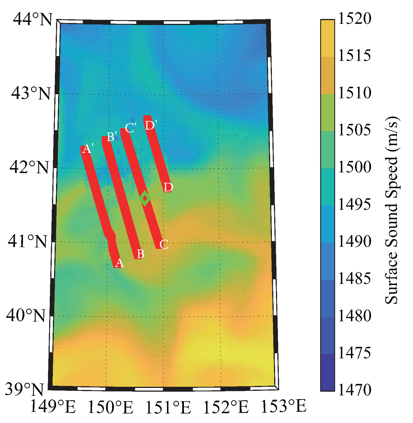
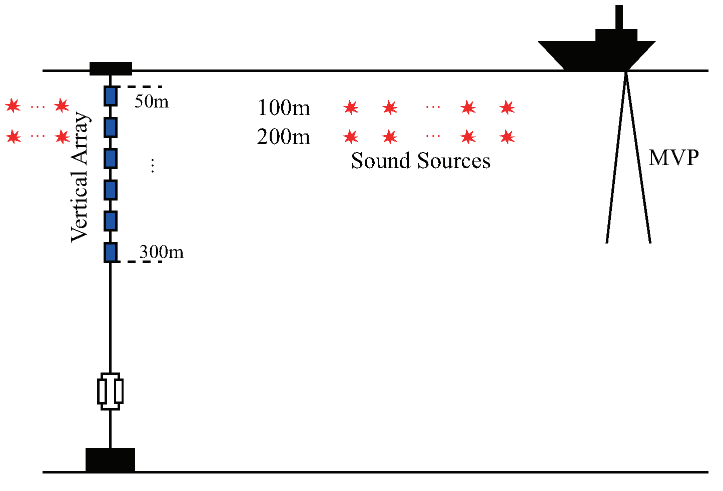
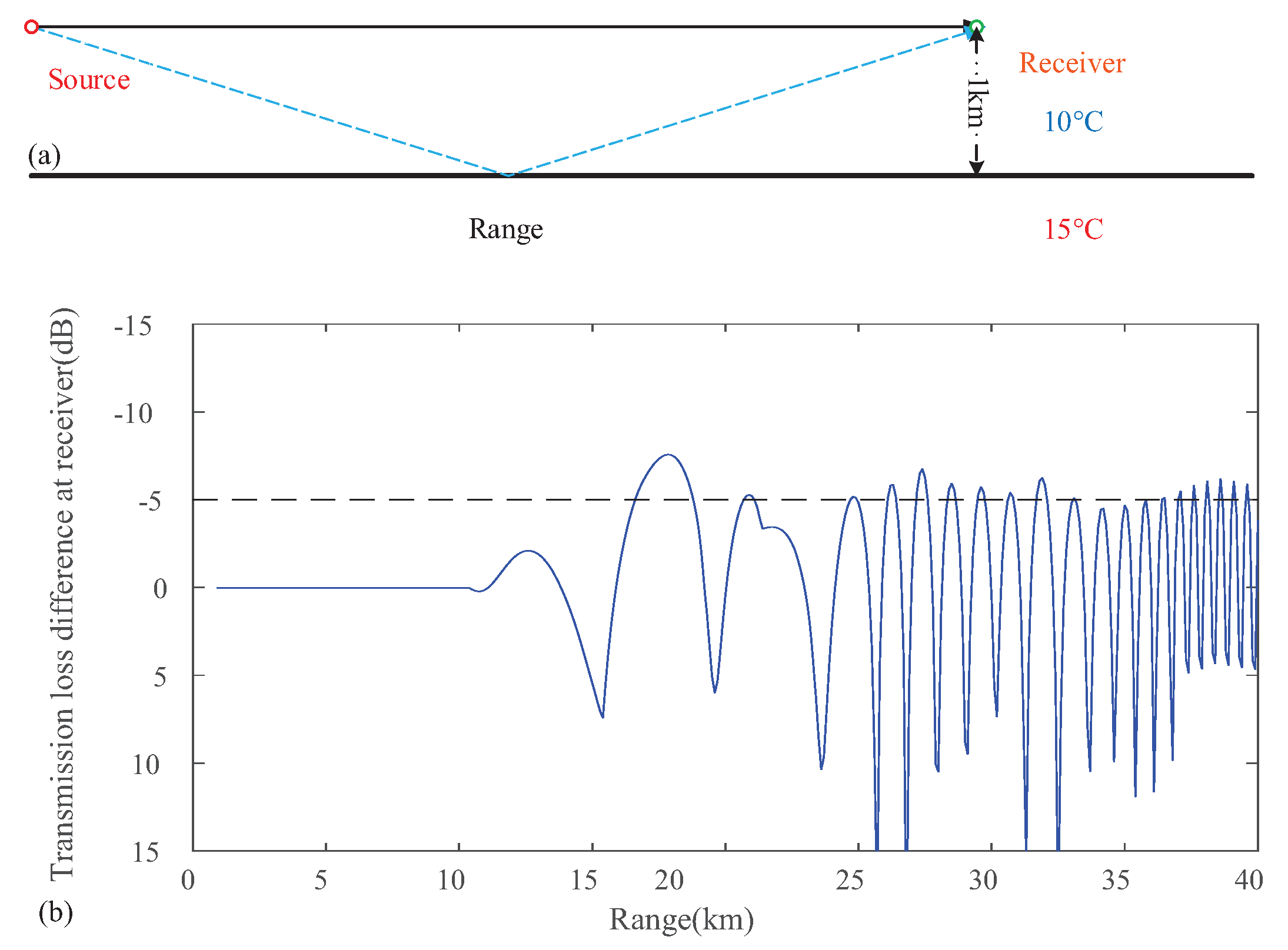
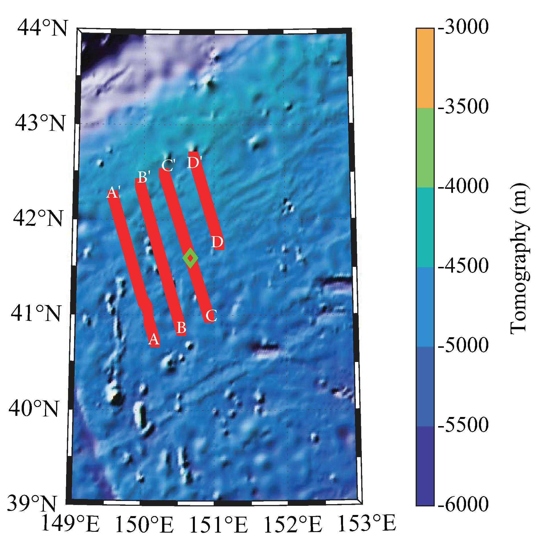
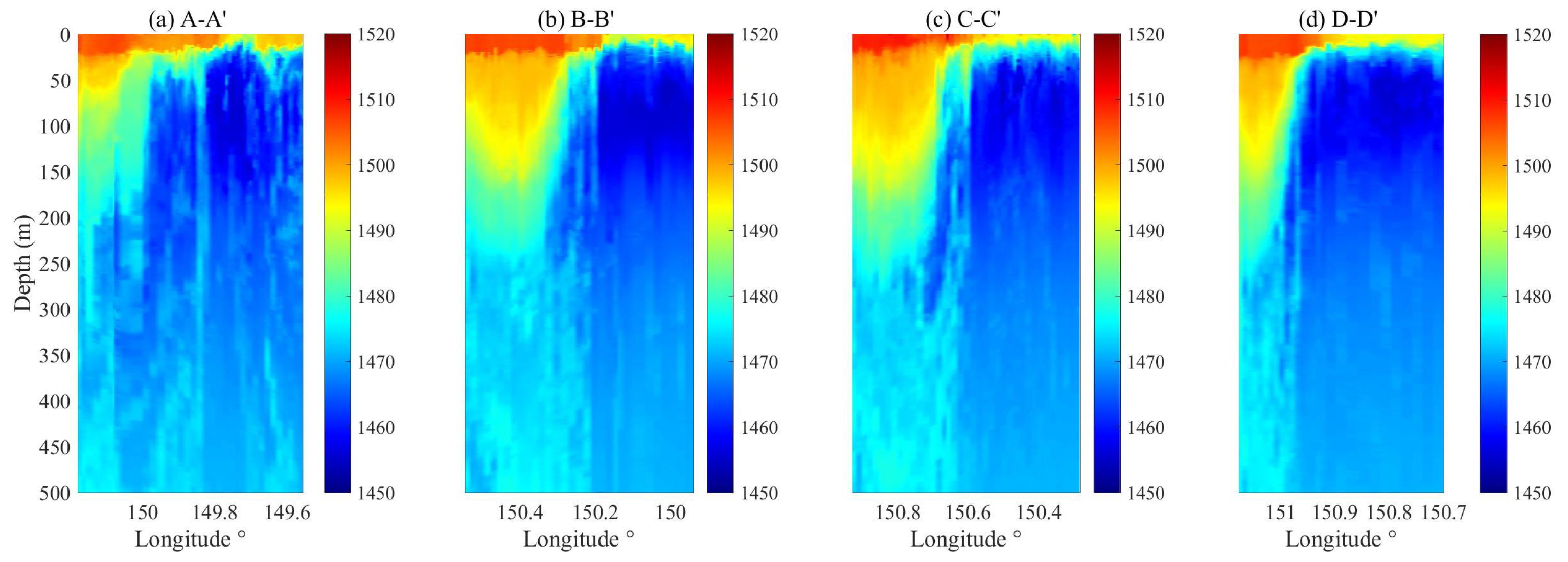
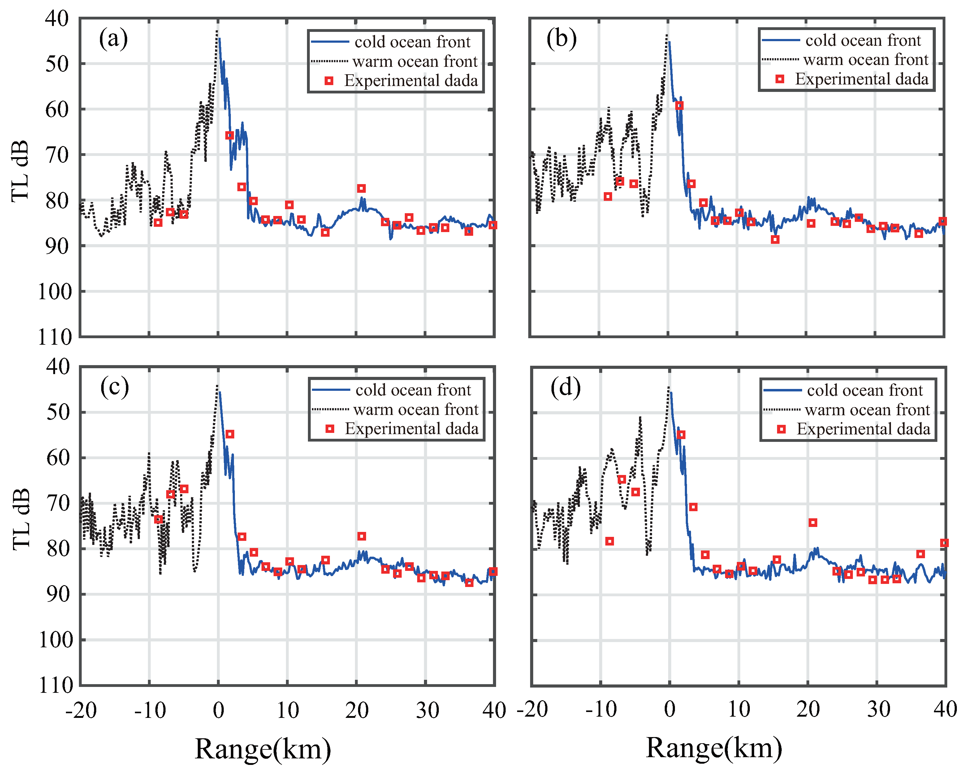
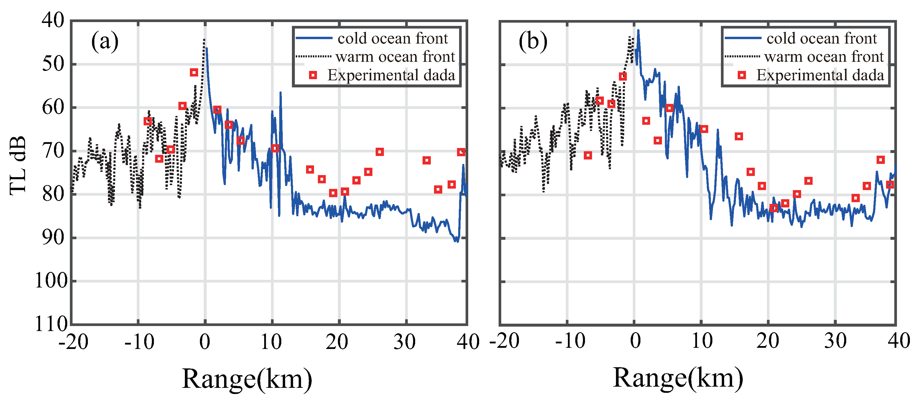
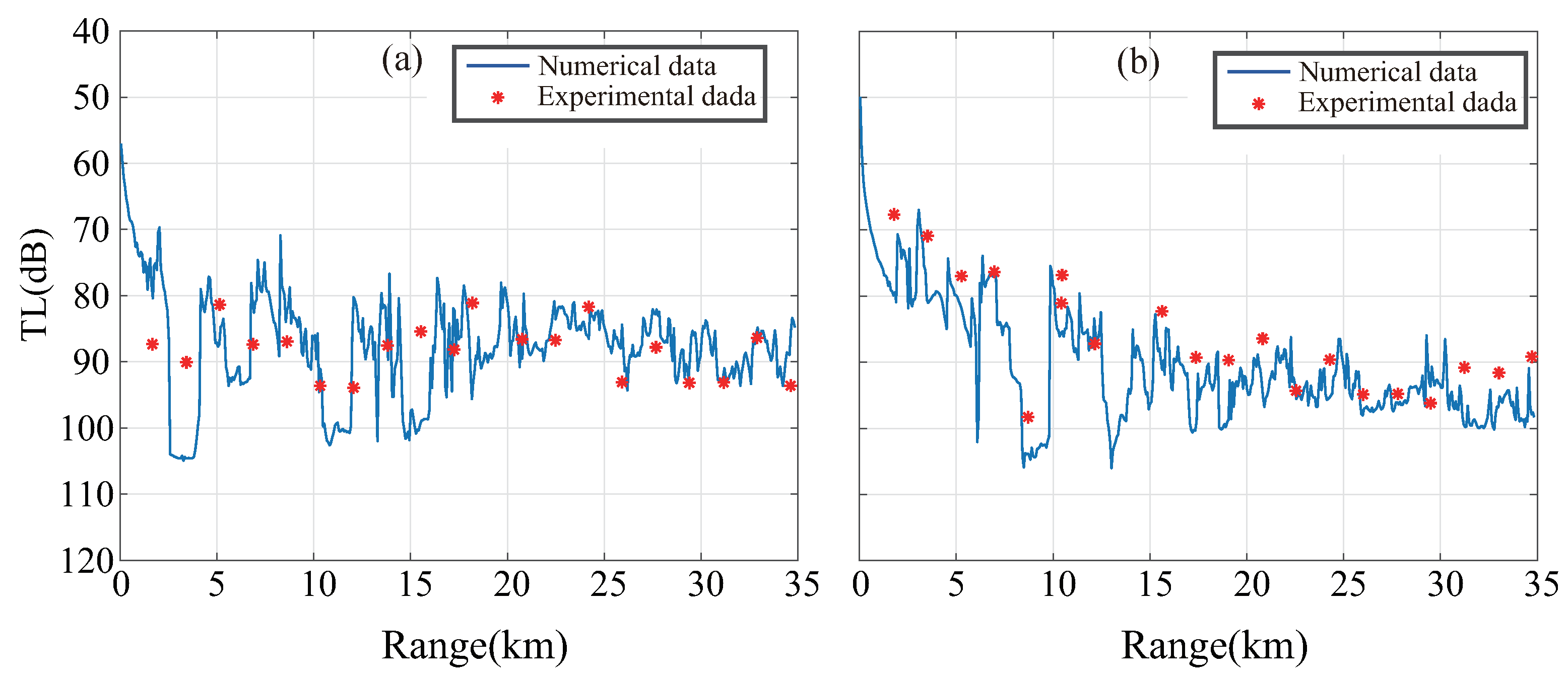
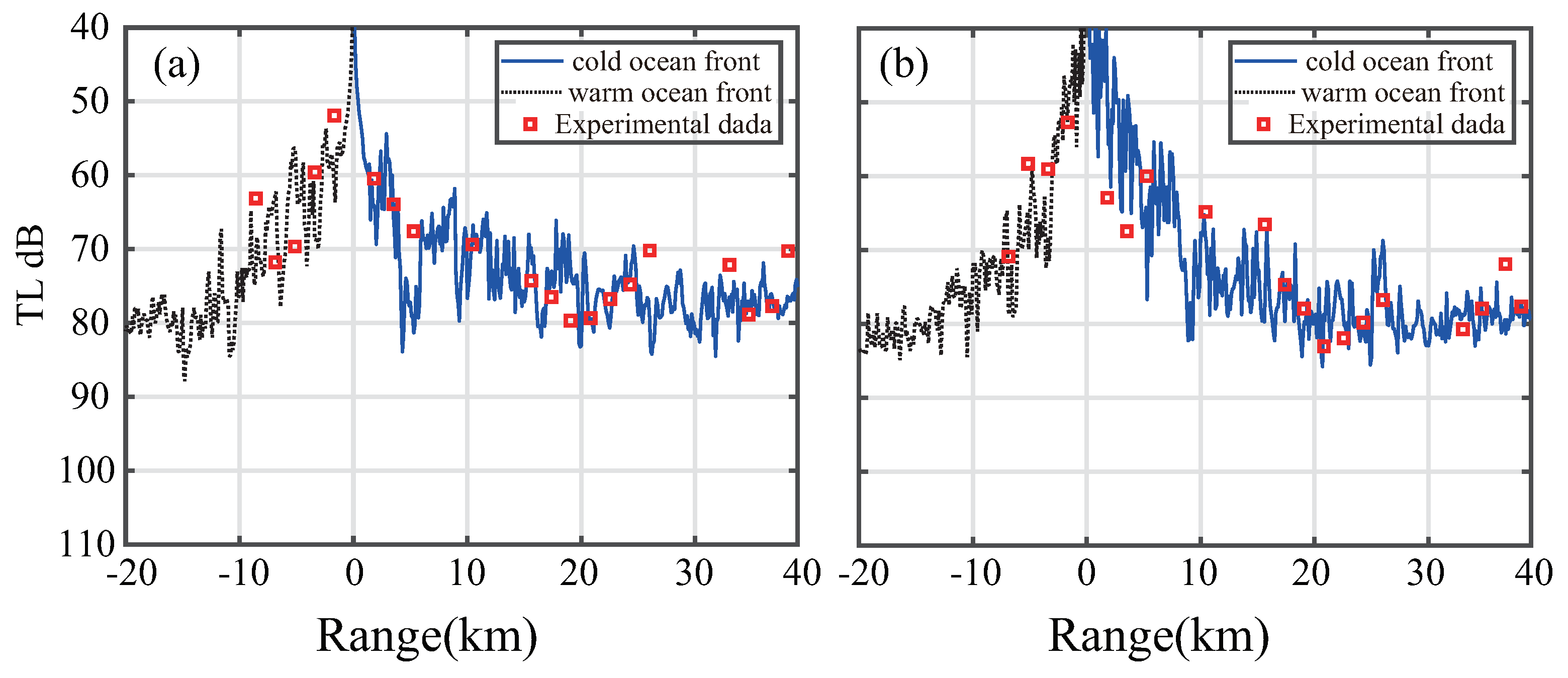
3. Comparison between Experimental and Numerical Simulation Results

The Kuroshio Current, one of the strongest surface oceanic currents in the whole ocean, intersects with the polar circulation and forms a large meander structure. The temperature and salinity distribution are extremely complex, especially in regions influenced by strong frontal currents. Nagai analysed the disturbance and temperature and salt distribution structure directly observed in the Kuroshio front sea area from the oceanographic perspective. Ocean energy dissipation is mainly influenced by the non-geotropic current and internal wave, with the changing of the temperature gradient [31]. The dynamic phenomena in the western North Pacific were identified and tracked, such as the size, life cycle and distribution of cyclonic and anticyclonic as respectively indicated in Figure 4a–d. The number of cold eddies and warm eddies in the western North Pacific are basically in the same magnitude, and the number of cyclonic is slightly larger.
From May to July 2019, a joint experiment of ocean acoustics and physical oceanography was carried out. The moving vessel profiler (MVP300) and conductivity-temperature-depth (CTD) measured the temperature/salinity gradients and sound speed profile. After four voyages along the ship trajectory, crossing the oceanic front, temperature and salinity data were collected continuously, which provided high-resolution environmental parameters for sound propagation study. Figure 5 shows the topography of the experimental area in the western North Pacific, the path of MVP300 (red lines) and the position of shipboard CTD cast (green rhomb) on 8 June. Figure 6 shows the sound speed of the ocean surface. The green rhomb and red lines are the locations of the CTD stations and MVP stations, respectively. Typical sound speed-depth curves were observed by underwater CTD in the western North Pacific, from 0 m to 2000 m in depth and deep oceans below 2000 m provided by remote sensing which is shown in Figure 7. Afterwards, Figure 8 illustrates four sound speed profiles in the water column collected by MVP.
We measured temperature variation in the horizontal direction, temperature and salinity consistently varied across the entire 3-D block, influenced by the warm Kuroshio current. The horizontal temperature gradient and salinity gradient between both sides of the oceanic front are large enough to detect the front, indicated in Figure 9a,b, respectively. The front has tracked to determine the placement of the receiving array for the following acoustic experiment. It is predicted that the frontal position located at 150.6° East longitude.
Putting the relationship of depth, salinity and temperature into the Equation (3) and calculating the variation of sound speed profile, Figure 10a shows a layered structure of the sound velocity in the water column. Due to warm-water mass intrusion, sound velocity changes in both surface layer and thermocline. Figure 10b exhibits sound velocity profiles at different longitude in order to describe sound speed layer structure more clearly. There is a minimum sound speed in SSP that varies from 1470 m/s to 1455 m/s at a depth of roughly from 300 m to 100 m. Meanwhile, the maximum sound speed and the sound speed near the seabed reach up to 1547 m/s.
The horizontal distribution of sound speed was obtained through interpolation. The horizontal and vertical coordinates are marked with longitude and latitude. The sound velocity distribution at a depth of 250 m is enlarged in Figure 11. It is intuitively noticed that the change of sound velocity of the oceanic front change dramatically below the mixing layer. In Figure 11, the geodetic longitude and latitude coordinates are converted to a Cartesian coordinate system, and the position (149° E, 39° N, z) replaced by the point (0, 0, z). This figure shows the three-dimensional temperature field at positions x = 10 km, x = 150 km and x = 340 km with a depth of 200 m. The solid black lines in the middle are the isotherm distribution of the temperature on the section. Vertical sections are the interpreted temperature profile in the distribution of uniform distance, and three layers are shown with the map of interpreted temperature at 0, 100 m and 200 m depths in Figure 12.
The following Figure 13 is a diagram of the sound propagation experiment configuration on the western North Pacific. The receiver system uses the ranges between a beacon fixed on the seabed and hydrophones on the submerged buoys aided by depthometers. There is a vessel in motion against the oceanic front. Melt cast explosives based on Trinitrotoluene (TNT) is used as high power and low-frequency underwater acoustic source. The transmission loss of sound pressure is acquired through theoretical calculations and experimental measurements. Two types of explosives are selected whose explosion depth is 100 m and 200 m. Moreover, more explosives occur on the side of the cold water as sound sources. The broadband explosives were thrown into the ocean every 1.7 km within 3 h from a vessel speed of 12 knots. The position of the blue rectangle is the vertical array of 10 self-contained underwater acoustic recorders, equally spaced from 50 m to 300 m. Figure 14 is one of the hydrophones used in this experiment, and the specifications of the hydrophones are shown in Table 1.
The actual depth of the vertical array influenced by ocean currents is not consistent with the preset values. After the depth of the vertical array was corrected, the receiving signals at the same depth were rearranged. The sampling frequency of the instrument is 10 kHz. To ensure the integrity of the received signal, the time window for intercepting the signal is selected according to the actual signal amplitude. The source signal spectrum was distributed from 5 Hz to 500 Hz, and the recorded signals were band-pass filtered with a Butterworth filter with a centre frequency of 120 Hz. The average coherence intensity of the sound wave is Equation (10). The pressure signal is also selected to have a peak frequency at 120 Hz and a 3 dB cut-off frequency from 106 Hz to 135 Hz. Ray theory is used to analyze the sound field and obtain broadband mean acoustic intensity by averaging the frequency points within the bandwidth in the interference field by Equation (10), where I is the sound intensity of the centre frequency of f 0 , Δ f is the half of frequency bandwidth.
I ( f 0 ) = 1 2 Δ f f 0 Δ f f 0 + Δ f p 2 ( f ) ρ c d f .
In this deep-sea sound propagation experiment, the acoustic reciprocity theorem was generalized for multiple sources and a fixed receiver array. In the sound field due to the source at explosive point, sound pressure received at any other hydrophones is the same as that would be produced at the explosive point if the source was placed at the depth of hydrophones. The results of signal processing received by different depth hydrophones are given by Figure 15. It can be seen from Figure 15a that there are no obvious differences for experimental results with different sound waves propagate direction (toward the cold side and the warm side), when the sound source was located in the mixed layer (75 m). However, it reflects the great differences that exist between the sound field propagated towards the warm and cold side of the ocean-front centre with three different depths of the acoustic sources located near the sound channel axis (150 m, 175 m and 200 m) is represented by Figure 15b–d. On the cold-water mass side, the distribution of the sound field is abnormal. There is a drop in the curves (after 3 km from the receiver array). On the contrary, transmission loss on the warm side of the oceanic front follows the law of reciprocal attenuation of the distance. These intuitive phenomena can be observed through the corrected experimental data and the sound pressure transmission loss curve drawn by simulation. Eventually, the agreement of experiment and modelling is satisfactory. At the bottom of the equipment, the float balls system is heavy enough for the vertical line hydrophone array to remain essentially in the experimental design. Although, the error may come from the fluctuation of the line array caused by the flow of the oceanic front. Figure 15 showed the calibrated depth of receiver hydrophone depends on the depth measurement. The standard deviation of explosion-signal receiver depths is within the allowed error range.
The whole depth of sound pressure transmission loss diagram is illustrated in Figure 16, simulated acoustic source located at depth of 175 m, the centre of the oceanic fronts is situated at the right cold side (red line in Figure 16). The warm water is on the right side of the front and the other side is cold. The sound field distribution on both sides of the oceanic front is discrepant. It is evident to observe that some acoustic rays turn downward until facing the centre of the oceanic front when the wave propagates to the right side, the other ray turning points. But on the other hand, there are no phenomena observed when the wave propagates to the left side. It can be concluded that the existence of the oceanic front does act as an acoustic lens that could strongly change the directions of acoustic propagation.
The data received on the hydrophone at 175 m depth were analysed, compared, and discussed here with the two-dimensional modelled result. Figure 17 indicates transmission loss generated by explosions at the depth of 200 m. The experimental data on the warm water side is in good agreement with the curve. Nevertheless, the 2-D simulation results at the side of cold water do not agree well with the experimental data. It is doubtful that the exciting sound pressure field at this depth is greatly affected by the horizontal refraction, which will be discussed in Section 4.
Designing a band-pass filter with a centre frequency of 200 Hz, and a 3 dB bandwidth of 50 Hz, comparing the difference in transmission loss between the two depths of explosions, the abnormal distribution of the propagation loss at 4 km and 8 km from hydrophone arrays can be observed by Figure 18. The rapid fall was also measured, as a result of the 200 Hz filtered experimental data. According to the propagation loss curve generated by the explosions at depth of 200 m, it can also be noticed that some data at some certain distance from the receiving vertical array does not match well.

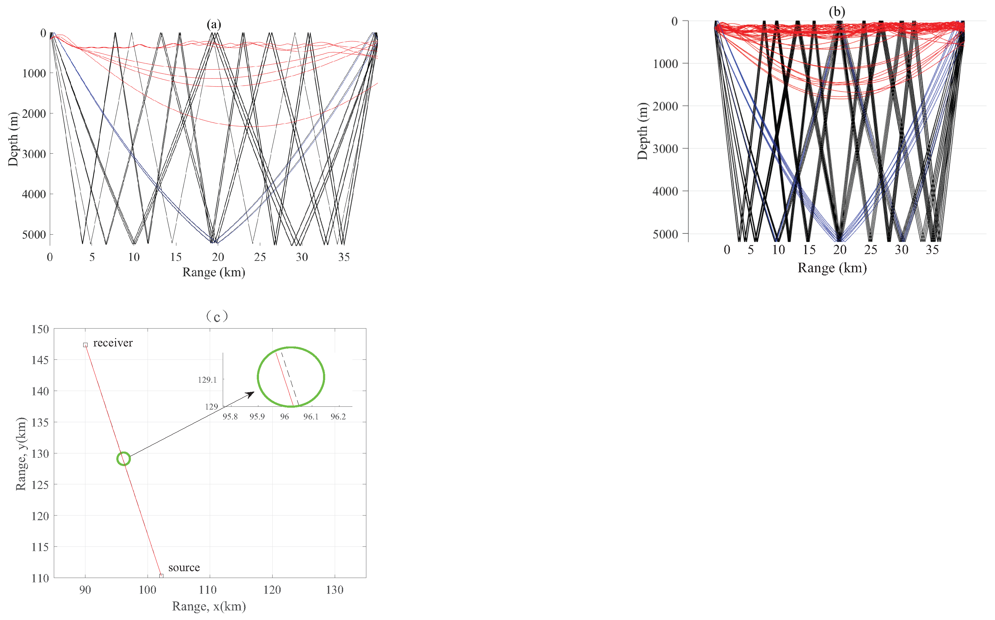
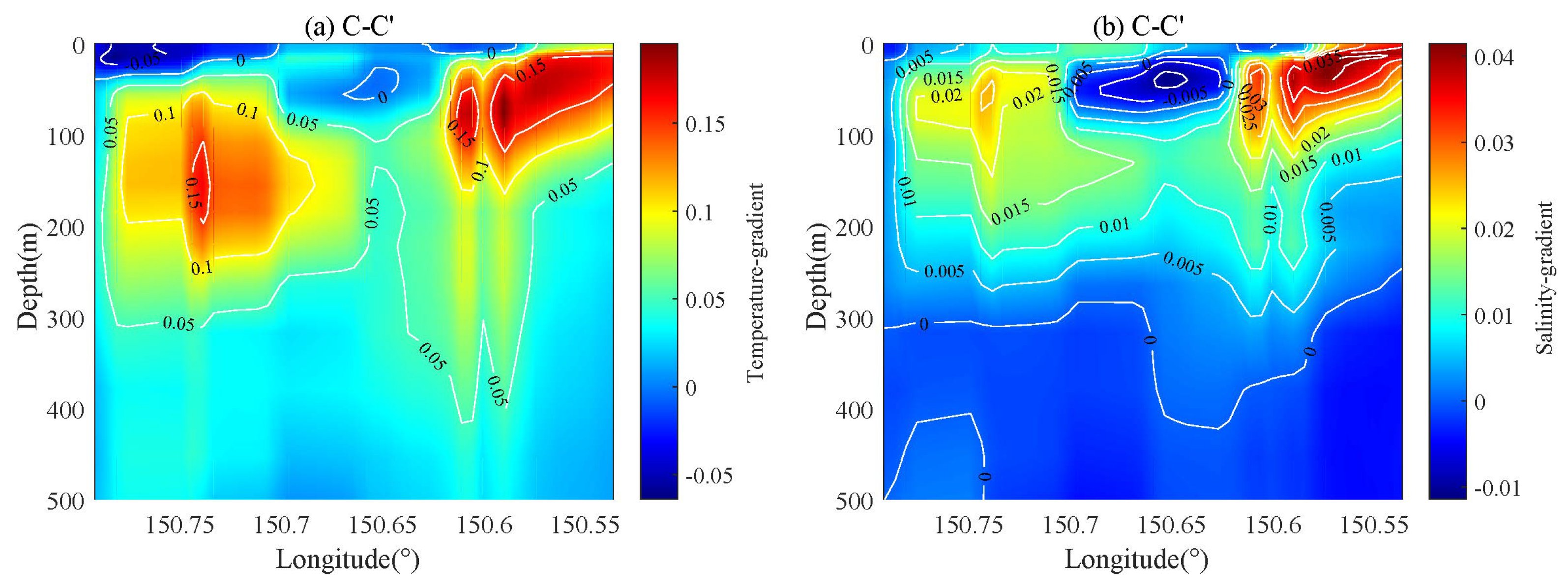
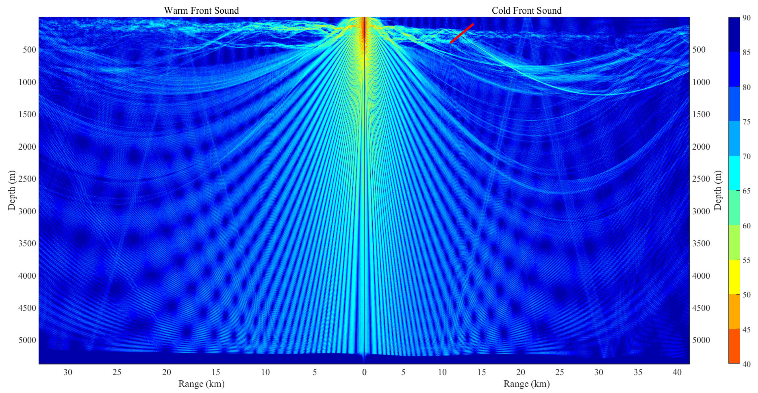
4. Discussion and Analysis Northwest Pacific Oceanic Front Sound Propagation and Horizontal Refraction Character

Both acoustic propagation direction and source position should be put into consideration when discussing the influence of ocean-front on the horizontal refraction of the acoustic field. In consideration of the deflection of acoustic rays in the two directions of the cold-water mass and the warm-water mass, the relationship between the maximum deflection angle of acoustic energy flow and the propagation distance is studied. The sound source propagates from the warm to the cold side, and more energy is confined to the mixed layer of the offshore surface. The horizontal refraction’s angle is the angle between the direction of the signal arrival at the point of reception and the true direction (the sound energy flow) to the sound source in the horizontal plane. The horizontal refraction’s angle symbol is also different from the thermocline, which is affected by the oceanic front. There is a misalignment between the direction of acoustic energy flow and the direction of the source to the receiver. Hence, positioning errors should be corrected when using horizontal energy flows to locate the source. This part is divided into three sub-problems for discussion. First of all, why are acoustic pressure transmission loss for the two sides of the oceanic front so different in the same receiver depth? Additionally, when the explosion source is located at 200 m depth, whether the three-dimensional simulation results are in better agreement with the experimental data than the two-dimensional simulation results? Eventually, sound wave propagation to the cold water side of the front is interpreted, using a 3D propagation model.

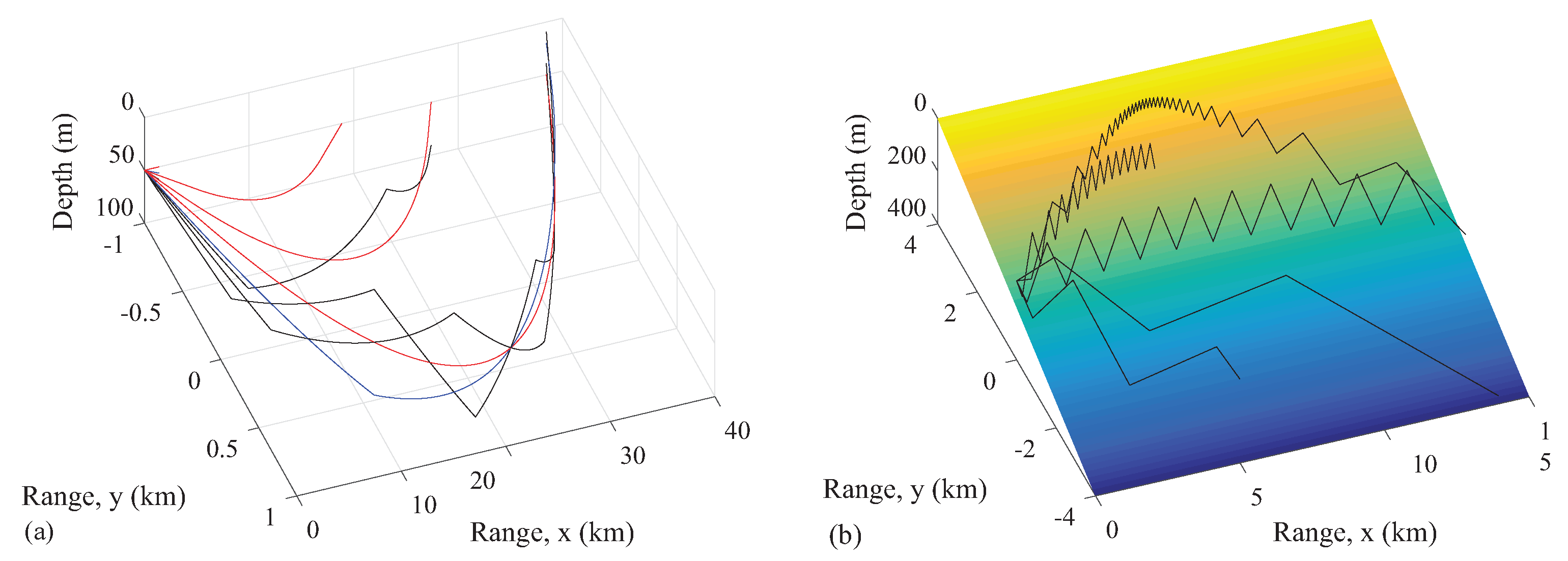
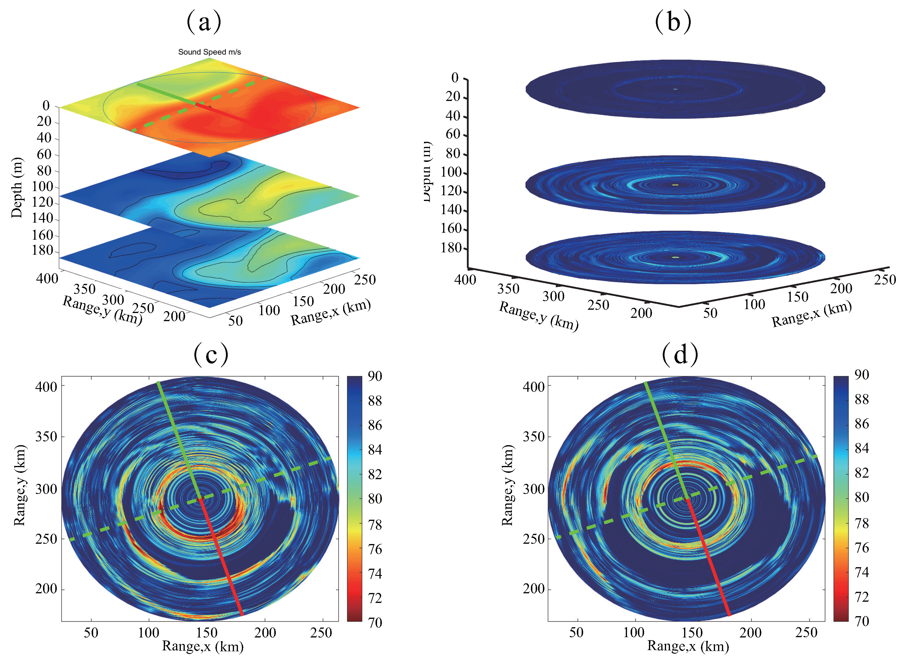
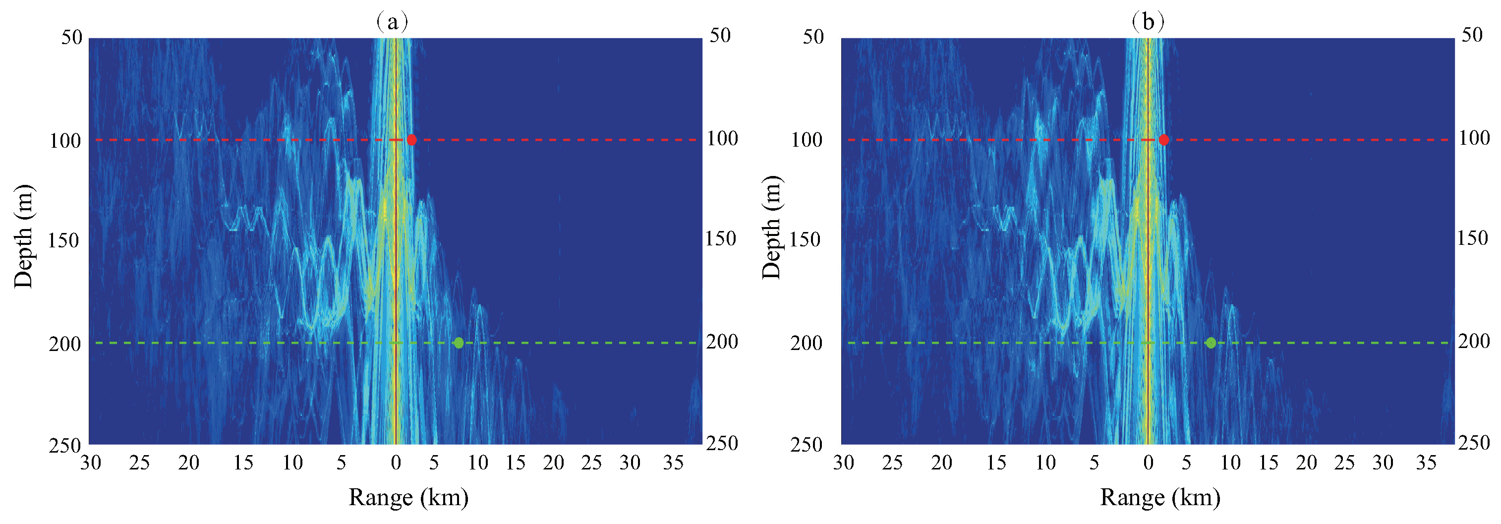
4.1. 3D Sound Propagation at Different Depths

The oceanic front is sloped, sound energy flow horizontal refraction is the most obvious of both sides of vertical direction with the strongest temperature gradient of the oceanic front. On the plane of the oceanic front, sound propagation away from front affected areas. According to the law of refraction, acoustic rays deflect to the area of the decrease of sound speed until the minimum of the temperature gradient occurs.
Topography is the controlled variable and is not allowed to change throughout the course of the simulation. The relationship between propagation attenuation and the oceanic front can quickly be established by changing the direction of propagation. The horizontal terrain with an average ocean depth of 5200 m is used for further simulation research. Figure 19a,b respectively show the sound speed top view from the sea surface at three depths and the sound pressure propagation loss in all directions which is excited by a sound source located near the centre of the front. To some extent, in Figure 19 green dotted line is the oceanic front, green solid line and the red solid line is regarded as the vertical directions of the oceanic front. In the Cartesian coordinate system with the sound source as the centre and the positive direction of the x-axis as 0 degrees, the direction of counterclockwise rotation of 72 degrees corresponds to the warm water side (red line), meanwhile the direction of anticlockwise rotation of 108 degrees corresponds to the cold water side (green line). To compare with Figure 19a,c, the oceanic front disturbs the distribution of the mixing layer. In the deep-sea mixed layer about 200 m as illustrated in Figure 19b, the sound pressure transmission loss at three depths illustrates an obvious difference. In the drawing, the green dotted line is the direction vertical to the oceanic front and the green solid line is the direction of the oceanic front. Figure 19 illustrates that with the effects of deep sound channel axis upward movement, when sound wave propagates to cold-water mass, more energy converges at the depth of 100 m under the sea surface; influenced by warm-water mass, sound channel axis is located under 200 m depth, and most of the acoustic rays skimmed over the sound channel axis region. With the increase of the transmission distance to the sound source, acoustic rays gathered in the deep-sea channel. Consequently, the cold side and the warm side are supposed to form concentric circles, a coherent circle of bright and dark with a similar distribution of sound speed appears.
Figure 20 shows the calculation results for 3D models at the depth of 175 m and 200 m, respectively. Comparing that with Figure 17 in the previous chapter, the tend of transmission loss curves basically agrees well with measurements. It’s important to notice that the curve drawn by the 3-D ray theory method is in better agreement with experimental data than that by the 2-D ray theory method. We probably indicate that it is caused by the horizontal refraction of the acoustic rays, namely the three-dimensional effect of the sound field. In the horizontal direction of the sound field excited by the explosions whose depth is 100 m, the bending of the acoustic rays is not obvious enough to affect the distribution of the sound pressure transmission loss. However, the horizontal refraction excited by the explosions whose depth is 200 m cannot be neglected.

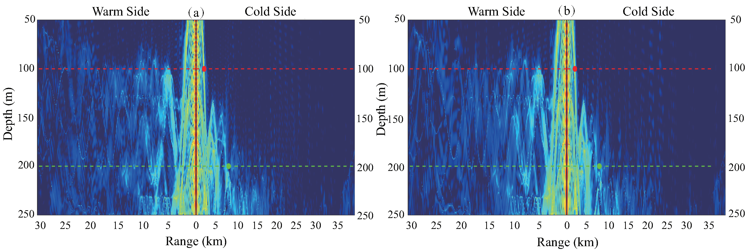
4.2. 3D Acoustic Ray Paths Explanations

There is no apparent difference between the curves of 2-D and 3-D simulation on the warm water side as shown by Figure 21a,b. The selective analysis is carried out by the changes of characteristic acoustic rays on the cold water side due to the influence of the oceanic front. Comparing the 2D model with the 3D model, there are more acoustic rays in the calculation process, and the sound pressure loses more energy with propagation illustrated in Figure 21. To observe the acoustic eigenrays, direct path arrival rays without surface-reflected and bottom-reflected rays represent more bending, which is the result of three-dimensional effects. At a distance of 27 km from the settled hydrophone receiver at the depth of 200 m, the 3D acoustic eigenrays have a unique convergence, and the unique convergence is not shown in the 2D simulation results, which also give evidence for Figure 17b and Figure 20b curve distinctions at the position of 27 km.

4.3. Interpretation of Acoustic Anomaly Distribution Use 3D Propagation Model

The sound wave propagation to both sides of the oceanic front is discussed using the 3D simulation, and whether the transmission loss curve anomaly at the position of 8 km in Figure 18 is also shed light upon. Figure 22 shows the two-dimensional simulation of transmission loss distribution on the acoustic experiment’s route. In Figure 23, the distribution of transmission loss is obtained from the three-dimensional simulation results of two excitation frequencies of sound sources. The red dotted line showing the sound pressure mutation is located exactly around 3 km away from the stationary as shown by the red circle in Figure 23a,b. The green dotted line showing the sound pressure mutation is located exactly around 8 km away from the stationary as shown by the green circle in Figure 23a,b. Whether the sound source frequency is 120 Hz or 200 Hz, the transmission loss at a depth of 100 m has no visible difference, while the transmission loss at 200 m depth displays a marked difference, especially at a long distance.

5. Conclusions

The Northwest Pacific oceanic front presented in this paper shows the significant effects of acoustic propagation in 2-D and 3-D models. As the common ocean dynamics phenomenon, it focuses the energy by horizontal and vertical plane refraction. The oceanic front changes the sound channel axis on both sides of the front centre. Especially on the cold water side, the sound channel is near the ocean surface which coincides with the depth interval of the mixing layer. The surface channel consists of a deep refracted path and several paths reflected from the surface and deeper upwards refraction. When the depth of hydrophone receiver is shallower than 150 m, transmission loss curves of the wave propagating to both sides of the oceanic front have the same tendency. However, when the depth of the hydrophone receivers is deeper than 150 m, there are significant differences between the curves in both directions. Comparison of diverse explosion depths by experiment expresses abnormal distribution of transmission loss, and yet anomaly position is uncertain. The decline of sonar action range owes to the oceanic front. More intuitively, the 3-D acoustic ray method is applied to study the acoustic ray paths which propagate from the explosion source towards both sides of the oceanic front. The comparison of the three-dimensional sound propagation between the experimental and numerical results illustrates that the three-dimension front environment should be considered when we discuss sound propagation and transmission loss at a depth of 200 m.
The horizontal refraction of acoustic rays carried out by front and undulated seabed are discussed. It is of interest to know how an oceanic front fell the amplitude of sound pressure at the cold water mass side. Furthermore, marine mammals nearby the sea surface could hardly be connected at some depth. Moreover, studying the effect of sound propagation could amend the inaccuracies of fish finders detection for the western North Pacific region. The additional advantage of studying horizontal refraction in the three-dimensional impact of the oceanic front is that the conclusion gives some idea and guides the placement of the vertical hydrophone array and tomography station. There are several alternative methods are available for solving these problems but spend much more time. Our further work is to overcome the slow computation and to expand our study to time-variant sound field characteristics with the existence of the oceanic front.

Author Contributions

Conceptualization, S.P.; methodology, J.L. and S.P.; software, J.L.; validation, J.L. and L.G.; formal analysis, J.L. and S.P.; investigation, J.L., L.G. and M.Z.; resources, S.P. and J.G.; writing—original draft preparation, J.L. and L.G.; writing—review and editing, J.L., S.P., L.G., S.Z., M.Z. and J.G.; visualization, S.P. and L.G.; supervision, S.P.; project administration, S.P.; funding acquisition, S.P. All authors have read and agreed to the published version of the manuscript.

Funding

This research was funded by National Natural Science Foundation of China, grant number 11904065.

Institutional Review Board Statement

Not applicable.

Informed Consent Statement

Not applicable.

Data Availability Statement

Not applicable.

Acknowledgments

The measuring of oceanic front data of the north-western ocean and the experiments of acoustic propagation were accomplished with the help of College of Meteorology and Oceanography in National University of Defense Technology.

Conflicts of Interest

The authors declare no conflict of interest.

References

  1. Bowman, M.J.; Esaias, W.E. Oceanic Fronts in Coastal Processes; Springer: Berlin/Heidelberg, Germany, 2012. [Google Scholar]
  2. Gangopadhyay, A.; Robinson, A.R. Feature-oriented regional modeling of oceanic fronts. Dyn. Atmos. Ocean. 2002, 36, 201–232. [Google Scholar] [CrossRef] [Green Version]
  3. Henrick, R.; Siegmann, W.; Jacobson, M. General analysis of ocean eddy effects for sound transmission applications. J. Acoust. Soc. Am. 1977, 62, 860–870. [Google Scholar] [CrossRef]
  4. Henrick, R.; Burkom, H. The effect of range dependence on acoustic propagation in a convergence zone environment. J. Acoust. Soc. Am. 1983, 73, 173–182. [Google Scholar] [CrossRef]
  5. Mahadevan, A.; Tandon, A. An analysis of mechanisms for submesoscale vertical motion at ocean fronts. Ocean Model. 2006, 14, 241–256. [Google Scholar] [CrossRef]
  6. Sokolov, S.; Rintoul, S.R. Structure of Southern Ocean fronts at 140 E. J. Mar. Syst. 2002, 37, 151–184. [Google Scholar] [CrossRef]
  7. Levine, E.R.; White, W.B. Bathymetric influences upon the character of North Pacific fronts, 1976–1980. J. Geophys. Res. Ocean. 1983, 88, 9617–9625. [Google Scholar] [CrossRef]
  8. Yang, W.; Li, B.; Gao, L.; Li, R.; Liu, C.; Ma, L. Ocean front locations in the southwest pacific. Chin. J. Polar Res. 2020, 32, 469–482. (In Chinese) [Google Scholar]
  9. Nakamura, H.; Inoue, R.; Nishina, A.; Nakano, T. Seasonal variations in salinity of the North Pacific Intermediate Water and vertical mixing intensity over the Okinawa Trough. J. Oceanogr. 2021, 77, 199–213. [Google Scholar] [CrossRef]
  10. Liu, Z.; Hou, Y. Kuroshio Front in the East China sea from satellite SST and remote sensing data. IEEE Geosci. Remote Sens. Lett. 2011, 9, 517–520. [Google Scholar] [CrossRef]
  11. Xie, L.; Pallàs-Sanz, E.; Zheng, Q.; Zhang, S.; Zong, X.; Yi, X.; Li, M. Diagnosis of 3D vertical circulation in the upwelling and frontal zones east of Hainan Island, China. J. Phys. Oceanogr. 2017, 47, 755–774. [Google Scholar] [CrossRef]
  12. Ying, K.; Linhui, P. Modal wave number spectrum for mesoscale eddies. J. Ocean Univ. Qingdao 2003, 2, 218–223. [Google Scholar] [CrossRef]
  13. Nakamura, Y.; Noguchi, T.; Tsuji, T.; Itoh, S.; Niino, H.; Matsuoka, T. Simultaneous seismic reflection and physical oceanographic observations of oceanic fine structure in the Kuroshio extension front. Geophys. Res. Lett. 2006, 33, L23605. [Google Scholar] [CrossRef]
  14. Neubert, J.A. Mean multipath intensity relation for sound propagation through a random ocean front. J. Acoust. Soc. Am. 1982, 72, 222–225. [Google Scholar] [CrossRef]
  15. Liu, Q. Research on Sound Propagation in the Ocean Mesoscale Phenomenon. Ph.D. Thesis, Harbin Engineering University, Harbin, China, 2006. [Google Scholar]
  16. Lee, D.; Saad, Y.; Schultz, M.H. An Efficient Method for Solving the Three-Dimensional Wide Angle Wave Equation; Technical Report; Yale University: New Haven, CT, USA, 1986. [Google Scholar]
  17. Wang, N.; Liu, J.Z.; Gao, D.Z.; Gao, W.; Wang, H.Z. An overview of the 2005 YFIAE: Yellow Sea Oceanic Front and Internal Waves Acoustic Experiment. J. Acoust. Soc. Am. 2008, 124, 2444. [Google Scholar] [CrossRef]
  18. Jian, Y.; Zhang, J.; Jia, Y. A Sound Speed Computation Model in Oceanic Front Area and Its Application in Studying the Effect on Sound Propagation. Adv. Mar. Sci. 2006, 24, 166–172. [Google Scholar]
  19. Guo, T.; Gao, W. Phenomenon of ocean front and it impact on the sound propagation. Mar. Forecasts 2015, 32, 80–88. (In Chinese) [Google Scholar]
  20. Chen, C.; Yang, K.; Duan, R.; Ma, Y. Acoustic propagation analysis with a sound speed feature model in the front area of Kuroshio Extension. Appl. Ocean Res. 2017, 68, 1–10. [Google Scholar] [CrossRef]
  21. Zhang, Y.; Yang, K.; Xue, R.; Huang, C.; Chen, C. Convergence zone analysis for a source in the front area of Kuroshio Extension based on Argo data. In Proceedings of the OCEANS 2019—Marseille, Marseille, France, 17–20 June 2019; pp. 1–4. [Google Scholar]
  22. Shapiro, G.; Chen, F.; Thain, R. The effect of ocean fronts on acoustic wave propagation in the Celtic Sea. J. Mar. Syst. 2014, 139, 217–226. [Google Scholar] [CrossRef]
  23. Calado, L.; Gangopadhyay, A.; Da Silveira, I. Feature-oriented regional modeling and simulations (FORMS) for the western South Atlantic: Southeastern Brazil region. Ocean Model. 2008, 25, 48–64. [Google Scholar] [CrossRef]
  24. Coppens, A.B. Simple equations for the speed of sound in Neptunian waters. J. Acoust. Soc. Am. 1981, 69, 862–863. [Google Scholar] [CrossRef]
  25. Jensen, F.B.; Kuperman, W.A.; Porter, M.B.; Schmidt, H. Computational Ocean Acoustics; Springer: New York, NY, USA, 2011. [Google Scholar]
  26. Hovem, J.M. Ray Trace Modeling of Underwater Sound Propagation. Documentation and Use of the PlaneRay Model; SINTEF: Trondheim, Norway, 2011. [Google Scholar]
  27. Porter, M.B. The Bellhop Manual and User’s Guide: Preliminary Draft; Technical report; Heat, Light, and Sound Research, Inc.: La Jolla, CA, USA, 2011; Volume 260. [Google Scholar]
  28. Porter, M.B. Beam tracing for two- and three-dimensional problems in ocean acoustics. J. Acoust. Soc. Am. 2019, 146, 2016–2029. [Google Scholar] [CrossRef] [PubMed]
  29. Červeny, V.; Pšenčík, I. Gaussian beams and paraxial ray approximation in three-dimensional elastic inhomogeneous media. J. Geophys. 1983, 53, 1–15. [Google Scholar]
  30. Lynch, J.F.; Colosi, J.A.; Gawarkiewicz, G.G.; Duda, T.F.; Pierce, A.D.; Badiey, M.; Katsnelson, B.G.; Miller, J.E.; Siegmann, W.; Chiu, C.S.; et al. Consideration of fine-scale coastal oceanography and 3-D acoustics effects for the ESME sound exposure model. IEEE J. Ocean. Eng. 2006, 31, 33–48. [Google Scholar] [CrossRef]
  31. Nagai, T.; Tandon, A.; Yamazaki, H.; Doubell, M.J.; Gallager, S. Direct observations of microscale turbulence and thermohaline structure in the Kuroshio Front. J. Geophys. Res. Ocean. 2012, 117, C08013. [Google Scholar] [CrossRef] [Green Version]
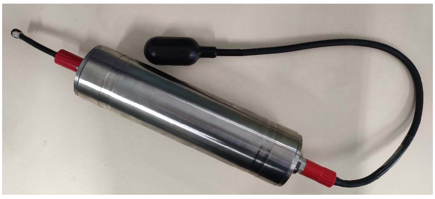
Figure 1. Vertical view of a simple velocity-based feature model of the temperature of front, x the dimensional along-front coordinate, y the cross-front coordinate with origin at the centre of the front and z the dimensional vertical coordinate (positive upward).
Jmse 09 01035 g001
Figure 2. (a) A simplified model of front environment source and receiver located 1 km from xz-plane and (b) frontal reflection effects on the sound pressure field, the curve is the difference transmission loss between a direct wave and a direct plus horizontal reflected wave.
Jmse 09 01035 g002
Figure 3. (a) Effect of a nearby oceanic front and (b) effect of a wedge seabed on horizontal refraction of the acoustic propagation.
Jmse 09 01035 g003
Figure 4. Statistical results of cyclonic and anticyclonic near Kuroshio obtained from 20 years of assimilation data from 1993 to 2014 (a) Kuroshio Current size (b) Kuroshio Current lifetime, (c) cyclonic size distribution and (d) anticyclonic size distribution.
Jmse 09 01035 g004
Figure 5. Topography of the western North Pacific. Colour shading indicates topographic relief from etopo1 data (global relief model of Earth’s surface, for more information https://www.ngdc.noaa.gov/mgg/global accessed on 1 April 2021).
Jmse 09 01035 g005
Figure 6. Sound speed of the ocean surface. Colour shading indicates sound speed fluctuation.
Jmse 09 01035 g006
Figure 7. Distributions of sound speed profile (blue solid line), temperature (red dash-dotted line) and salinity (pink dashed line) for the depth from the ocean surface to bottom at the position of CTD.
Jmse 09 01035 g007
Figure 8. Measured sound speed profile from (ad) is the survey line A–A , B–B , C–C and D–D , respectively, which are marked in Figure 5.
Jmse 09 01035 g008
Figure 9. Distributions of temperature (a) and salinity (b) gradients.
Jmse 09 01035 g009
Figure 10. Distribution of sound speed profile on Longitude and depth, (a) vertical slice map and (b) Those sound speed profiles are equally divided into 20 slices in 60 km of range, green line shown the position of oceanic front and blue dot is the sound channel axis.
Jmse 09 01035 g010
Figure 11. Regional sound speed profile for the depth of 250 m.
Jmse 09 01035 g011
Figure 12. Three-dimensional temperature structure of the front transect. (ac) are slices of the temperature in the yz plane, xz plane and xy plane, respectively.
Jmse 09 01035 g012
Figure 13. Experimental installation in the western North Pacific.
Jmse 09 01035 g013
Figure 14. Hydrophone: signal conditioning, low-noise cable and data acquisition.
Jmse 09 01035 g014
Figure 15. Transmission Loss in cold side (blue dotted line), warm side (black line) and experimental results with 100 m explosions (red square) in depths of 75 m (a), 150 m (b), 175 m (c) and 200 m (d).
Jmse 09 01035 g015
Figure 16. Transmission Loss in both warm and cold sides of oceanic front.
Jmse 09 01035 g016
Figure 17. 2-D Transmission Loss in cold side (blue line), warm side (black dotted line) and experimental results with 200 m explosions (red square) in depths of 175 m (a) and 200 m (b).
Jmse 09 01035 g017
Figure 18. Comparison of Transmission Losses between numerical and experimental results for 175 m depth of hydrophone, (a) explosive source at depth 100 m and (b) at 200 m.
Jmse 09 01035 g018
Figure 19. (a) Three dimensional structure of the oceanic front, (b) Transmission Losses 3-D for depths 0 m, 100 m and 200 m, (c,d) Transmission Loss slice for depth 100 m and 200 m.
Jmse 09 01035 g019
Figure 20. 3-D transmission loss in cold side (blue line), warm side (black dotted line) and experimental results with 200 m explosions (red square) in depths of 175 m (a), 200 m (b).
Jmse 09 01035 g020
Figure 21. Comparison of sound rays between in (a) 2-D and (b) 3-D environment. Subfigure (c) is the top view of sound rays in 3-D simulation which showed horizontal refraction phenomenon. In the picture, red solid line is the acoustic ray and black dotted line is direction from source to the receiver.
Jmse 09 01035 g021
Figure 22. 2D simulation of sound pressure transmission loss at the frequency of (a) 120 Hz and (b) 200 Hz.
Jmse 09 01035 g022
Figure 23. 3D simulation of sound pressure transmission loss at the frequency of (a) 120 Hz and (b) 200 Hz.
Jmse 09 01035 g023
Table 1. Hydrophone specifications.
Parameter TypeParameter Value (Range)
Frequency Range10 Hz–20 kHz +3/−3 dB
Receiving Sensitivity−203 dB re 1 V/ μ Pa
Amplification Gain20 dB
Filter Bandwidth20 kHz
Sampling Rate10 kHz 24 bit
Network Specific Interfaces100 M/10 M Based TCP/IP
Supply Voltage and Current19 V DC and 2 A
Publisher’s Note: MDPI stays neutral with regard to jurisdictional claims in published maps and institutional affiliations.

