Express Image and Video Analysis Technology QAVIS: Application in System for Video Monitoring of Peter the Great Bay (Sea of Japan/East Sea)

Abstract

The article describes the technology of express analysis of images and videos, recorded by coastal video monitoring systems, developed by the authors. Its main feature is its ability to measure or evaluate in real time the signals of sea waves, sea level fluctuations, variations of underwater currents, etc., on video recordings or streaming video from coastal cameras. The real-time mode is achieved due to processing video information read not from files, but from the graphic memory of the screen. Measurements of sea signals can be carried out continuously for a long time, up to several days, with high sampling rate, up to 16 Hz, at several points of the observed water area simultaneously. This potentially allows studying the entire spectrum of wave movements, from short waves with periods of 0.3–0.5 s to multi-day fluctuations at the sea level of a synoptic scale. The paper provides examples of the use of this technology for analyzing images and videos obtained in the network of scientific video monitoring of the Peter the Great Bay (Sea of Japan/East Sea), deployed by the authors.

1. Introduction

Systems for long-term video surveillance of coastal waters have been actively deployed around the world since the early 2000s. A great contribution to this process was made by the activities of the scientific group of R. Holman from the Coastal Imaging Lab (CIL) at Oregon State University, which was engaged in the development and application of photo and video equipment for studying the morphodynamics of sea coasts since the early 1980s [1,2]. In 1992, they developed and tested a standard coastal video surveillance system, ARGUS [3]. Information from 5–6 cameras was used for long-term monitoring of dynamic processes in the coastal zone of the sea, which affect the coastline. Quantitative methods were developed for describing hydrodynamic and morphodynamic processes in the surf zone based on the analysis of ARGUS video data [4,5,6]. Later, more than 30 such complexes were deployed in several countries around the world as part of the international CoastView project [7]. Data from all stations were promptly sent to the Internet network, for example, on the CIL website (http://cil-www.coas.oregonstate.edu/, accessed on 26 July 2021). It helped to popularize the project and stimulated the deployment of remote scientific video surveillance systems for coastal waters in different countries, including those not covered by the ARGUS network.

Largely under the influence of CoastView, in 2007, it was decided to start deploying a network of integrated scientific video surveillance systems of one of the most important water areas of the Far Eastern region of Russia—Peter the Great Bay—located in the southern part of the Primorsky Krai. The network was supposed to be an important part of the Scientific Monitoring System (SMS) of the Bay, launched in the Pacific Oceanological Institute of the Far Eastern Branch of the Russian Academy of Sciences (POI FEB RAS) in 2005. The developers of QAVIS-technology were engaged in the deployment of the SMS “cyberinfrastructure”—a set of technical and software tools for the quick delivery, processing, and presenting to scientists of data from several monitoring experiments conducted by scientific groups of POI FEB RAS. The data of the coastal video surveillance, organized at key points of the Bay, was to significantly supplement the SMS databases with information that would be useful in interpreting all other scientific data collected in the system. This determined the main tasks of the video monitoring system (VMS): 1—collecting, storing, and providing scientists with operational and historical video data on the state of the Bay’s waters, 2—developing and applying in research video-based methods for quantitative assessment of the parameters of sea processes—currents, sea-level fluctuations, and others.

The QAVIS program (Quick Video and Image Analysis for Scientists) has proven useful in performing the second group of tasks. It allows one to measure, in several local points of the observed water area, wave signals h(t) or other signals, for example, the signal of the sea surface brightness B(t), carrying information about the properties of h(t), from sea video recordings or directly from video streams. Signal measurements can be made with a frequency of up to 16 Hz, continuously, for a long time, up to several days. This potentially makes it possible to analyze the entire spectrum of wave processes in the water area, from short wind waves to synoptic sea-level fluctuations. QAVIS is complemented by Stitcher and OceanSP. The first one allows stitching the signals received in QAVIS with other geophysical signals into a single multi-channel file. OceanSP provides a set of tools for analyzing such multi-channel signals. The complex of programs presented in this paper, together with the methods of their application, is proposed as QAVIS-technology for studying sea processes based on coastal videos.

The article will provide information about Peter the Great Bay VMS, QAVIS technology, and its capabilities in studying wave processes and sea-level fluctuations based on VMS data.

This article examines several examples of the use of QAVIS in measuring the characteristics of wave processes and evaluating their frequency properties. In some cases, these measurements were compared with data from alternative surveillance tools, which, in general, confirmed the objectivity and effectiveness of the corresponding QAVIS measurement techniques. In other cases, it was not possible to obtain data from alternative measuring instruments for various reasons. In these cases, it cannot be stated that the accuracy and efficiency of QAVIS measurements are fully proven. The presentation of such techniques in the article is justified since they determine the directions for future research of promising measuring techniques using QAVIS and professional oceanographic instruments.

2. Material and Methods

2.1. Peter the Great Bay Video Monitoring System

As of 1 January 2018, the VMS consisted of twelve surface and three underwater cameras installed in 7 geographical points on the coast and islands of Peter the Great Bay and on two small research vessels (see the locations of installation sites in Figure 1).

At point 1 (the roof of the POI FEB RAS building), up to three stationary and PTZ cameras with a view of the waters of Amurskiy Bay worked at different times. PTZ cameras, under the control of the operator or program, could be rotated horizontally (Pan) and vertically (Tilt) and change the multiplicity of optical zoom (Zoom) by increasing or decreasing the focal length of the lens. At point 2 (Marine Experimental Station (MES) “Alekseev Bay” on Popov Island), two surface and two underwater cameras were used. PTZ camera Axis-233d provided a 360° view of the waters around the island. The stationary surface camera in Alekseev Bay was used as part of the “videowavemeter”. Underwater cameras were located on the bottom of Alekseev Bay, at 100 and 200 m from the shore. At point 3 (Marine Station of the Institute of Marine Biology FEB RAS in Vostok Bay), a stationary IP camera was used to view the nearest water area from 2014 to 2018. At point 4 (scientific cordon of the Far Eastern Marine Reserve on the Bolshoy Pelis Island), from 2014 to 2020 there was an IP camera with a view of nearby water areas. At point 5 (Marine Station “Cape Schultz”) in the Posyet Bay, from 1 to 3 surface cameras and one underwater camera were used at different times. At point 6 (Marine Reserve cordon on the Furugelm Island), a stationary camera was installed, with a view of the Posyet Bay water area in the direction of Cape Schultz. Point 7 indicates the location of two small research vessels of the Institute, on which one stationary camera and one PTZ camera were installed.

Information from all cameras, along with data from other remote scientific observations, was sent, on the set schedule, to the SMS databases (DB). From each stationary camera, one snapshot per minute and one-minute-long video per hour were entered into the DB. Day-long animations were compiled from the snapshots and were also saved in the SMS database. PTZ cameras additionally make a 360° view of the water areas every hour and send snapshots to form panoramic images on the SMS computing servers. Every day, 10–20 GB of video data were stored in the DB. About 30 Terabytes of video data were collected between 2009 and 2021. To request video data, the Institute’s researchers used the corporate web service of SMS inaccessible from the outside. A separate web service had been developed for open access to data from several cameras (https://poi.dvo.ru/live/, accessed on 25 September 2021). The state of the VMS by 2011 is described in [8].

Institute staff analyzed images and videos from SMS databases using professional programs, such as Adobe Photoshop and Adobe Premiere Pro, and also the QAVIS program. The latter can analyze not only previously recorded video files, but also live video streams simultaneously from several cameras in real time. Figure 2 shows the process of analyzing “live video” from 7 cameras installed in 6 points of the bay. Three computers were used: 4 streams were processed on the first one, 2 on the second, and 1 on the third computer. The number of camera installation locations is indicated on each stream, in accordance with Figure 1. Estimates of the wave signal (for cameras 1, 2, 4) or signals that carry information about the frequency properties of the wave signal (for cameras 3, 5, 5′, 6 were measured. Continuous measurements with a sampling frequency of 2 Hz were carried out in the summer of 2017 for more than 40 days. Swell waves arriving in the bay from the central and northern parts of the Sea of Japan were recorded several times during the measurement period. They were recorded at all points simultaneously and had the same base periods from 5 to 12 s. Wind wave spectra varied significantly at different points, as they are determined by local wind conditions.

2.2. Sources of Geophysical Data, Used for Interpretation of QAVIS Video Analysis Data

The validation of the QAVIS methods for the analysis of coastal wave processes was carried out using synchronous geophysical observations performed in SMS or freely available on the Internet data from other organizations. Two automatic weather stations were located in points 2 and 5 (numbers as in Figure 1). The most important meteorological parameters for checking QAVIS methods are wind direction, wind speed, and atmospheric pressure. Sea level measurement stations, included in the Global Sea Level Observing System (GLOSS), were installed in Vladivostok, Posyet Bay, and Nakhodka (http://www.ioc-sealevelmonitoring.org/station.php?code=vlad, accessed on 25 September 2021). Measurements were carried out once per minute with an accuracy of 1 cm.

In 2008, specialists of the Kamchatka branch of the Unified Geophysical Service of the Russian Academy of Sciences installed the CMG-3ESPB broadband seismic station in point 5 on Cape Schultz. Its unique feature is its proximity to the coastline (distance—150 m), facing the open part of the Sea of Japan. As previous QAVIS observations show, swell waves entering the bay (typical periods of 5–14 s) can usually be detected simultaneously in wave signals and primary microseisms [9] of the seismic station’s BHN channel. This channel registers the earth’s surface vibration velocity along the “North-South” direction, facing the open part of the Sea of Japan. Primary microseisms are caused by swell waves running up to the coast of the cape, so their period coincides with the swell period. In addition to primary microseisms, the seismic signal contains more powerful secondary microseisms, the frequency of which is equal to twice the frequency of the swell waves. They arise due to the fields of standing waves caused by the superposition of direct and reflected from the cape waves. These standing waves send pressure pulses towards the seabed with a frequency twice that of the original swell wave. This causes secondary microseisms that propagate along the seabed in the form of Rayleigh waves in all directions, including towards the seismic station at Cape Shultz. Swell is a large-scale process; when it comes from the central part of the Sea of Japan to Peter the Great Bay, it manifests itself in all its local waters. Therefore, seismic data were used in the most difficult cases, for example, when studying the ability of QAVIS to register sea waves at long distances from the camera, up to 5 km.

In the same place, at Cape Schulz, two instruments were installed: a laser-interference complex, consisting of two laser strainmeters measuring oscillations of the earth’s surface in the frequency range up to 1000 Hz in the North–South and East–West directions, and a laser nanobarograph, measuring fluctuations in atmospheric pressure [10,11]. They were used for comparison with QAVIS data in the range of wind and infragravity waves. Moreover, the POI FEB RAS has developed several designs of laser-interference meters for hydrospheric pressure variations–laser hydrophones [12,13]. They were installed at various points in Peter the Great Bay and registered variations in the hydrosphere pressure in the frequency band from 0.00001 to 1000 Hz. They were used for comparison with QAVIS data in the range of surface waves and seiche sea-level fluctuations.

Furthermore, data from satellite observations of the waters of the Sea of Japan, available on the Internet, were used to verify the results of QAVIS measurements. The most commonly used images of the sea surface are in the visible and radar ranges from the Sentinel-2 satellite, provided by the Sentinel-Hub EO Browser of the European Space Agency (EO Browser, Sinergise Ltd., https://apps.sentinel-hub.com/eo-browser/, accessed on 25 September 2021). In turn, specialists in satellite methods used data from QAVIS measurements of wave processes to interpret satellite information.

2.3. QAVIS Technology Software

The software consists of three programs: QAVIS, Stitcher, and OceanSP. The first one analyzes images or videos and, if necessary, stores the output spatial or temporal signals in text or binary files. Stitcher stitches QAVIS signals and any other time-synchronized geophysical signals into single multi-channel signals. The text format of the output files is simple; they can easily be processed in any software system for scientific calculations, for example, in Matlab. In this paper, another program, OceanSP, is presented. It implements many signal processing algorithms and works with the QAVIS data formats or data in text files.

Let’s now take a closer look at the main program-QAVIS (Quick Analysis of Videos and Images for Scientists). It was developed as an easy-to-use program for scientists from any field of research that deals with images or videos. When working at a computer, scientists can notice spatial or temporal patterns in pictures and videos. They may have ideas on how these patterns can be quantitatively described and applied in their professional activities. With the help of QAVIS, they can very quickly go to the practical investigation of assumptions and ideas directly on the observed image or video. Another important aspect of QAVIS quickness is that video processing is done in real time. Analysis of marine video surveillance data is one of the possible areas of application for QAVIS.

The program is compact; it consists of three files with a total volume of about 2 MB. It works on ordinary personal computers, running Windows XP, Windows 7, Windows 10. It requires the Microsoft.NET Framework package installed on the system, no lower than version 4.1. It is usually pre-installed with the operating system or can be downloaded from the Internet. QAVIS, like OceanSP, uses the fast Fourier transform library FFTW (http://www.fftw.org/, accessed on 25 September 2021). The QAVIS software, along with OceanSP and Stitcher, can be downloaded from the web page (http://oias.poi.dvo.ru/qavis/, accessed on 25 September 2021).

The main feature of the program is that it does not work with image and video files, but with information that is currently displayed on the computer screen. QAVIS reads static images and video frames from the screen’s graphics memory. If visualization of information from some source file on the computer screen is performed at the scale of 1:1 (this can always be controlled), then the array of pixels $x\left(i,j\right), i=\overline{1,N}, j=\overline{1,M}$ read from a rectangular area of the screen of size N × M, is in most cases completely identical to the array of pixels in the file. In both cases, one pixel is encoded with three bytes that carry information about the intensity of the red (R), green (G), and blue (B) components of its color. If the scale is different, then the user decides how critical this is for analysis. When working with video in the QAVIS program, the user sets the frame processing frequency (FPS—frames per second) from the range 1–64. It defines the time interval between frame processing cycles: T = 1/FPS. If one frame is processed in a timeframe less than T, the real-time mode is achieved, and the results will be the same as when processing video files. Thus, replacing work with files with work with screen memory does not lead to information losses. The user’s convenience is obvious. They do not have to look for ways to download a file image of a video of interest from the Internet, deal with video data storage formats, or look for suitable software for processing. The price of such convenience is that many of the functions supported in professional image and video processing programs are not implemented in QAVIS. However, as the experience of using the program shows, the functions available in it are enough to solve many practical tasks of sea video monitoring.

When loading QAVIS, a small window appears that is always displayed on top of all other windows, and is opened by the user (Figure 3).

If necessary, important parameters of the program can be modified in the Settings section. QAVIS works only with scalar images, by default, grayscale (gray). Each pixel is assigned a scalar value, composed of three-color components according to the rule $x=\left(R+G+B\right)/3$. In the settings, users can select the mode of operation with only one color component: R, G, or B. Moreover, the frequency of data processing cycles is set in the settings, FPS. Several options are offered: 1, 2, 5, 9, 16, 21, 32, 64. For sea video monitoring, the FPS = 5 option is usually sufficient. In this case, the program allows one to analyze wave processes with periods of 0.4 s or more. In the settings, the user can set a scale by specifying the linear size of one pixel. Another important parameter is enabling/disabling the display mode of auxiliary markers on the image. Such markers (vectors of movement of objects on the water surface, vectors of wave velocity, schematic representations of wavefronts, etc.) are used for visual control of the correct operation of QAVIS tools, but sometimes interfere with a visual observation of the scene itself.

In general, there is one technical problem associated with the display of auxiliary markers on top of the image, which users should take into account. Due to the peculiarities of operating systems, such displays that do not distort the main image under the markers cannot be implemented in Windows 10. QAVIS recognizes this situation and makes auxiliary displays in separate information windows.

To analyze the images and videos observed on the computer screen, QAVIS presents four tools: Brightness, Transect, Correlation, and Spectrum, which are called from the initial window (Figure 4). Each tool has its own “selector” with which the user specifies the area of analysis on the computer screen. At the beginning of each clock cycle, the program reads the information under each selector from the screen, performs the appropriate processing, and displays the results in small information windows. Often, this information is sufficient for analyzing video data. In other cases, the user can record the signals produced by the tools to files that can be analyzed, after the recording is completed, by the user’s programs, or by using OceanSP. In Figure 4, all four types of instruments are installed in the sea surface video viewer window after a ship passes from left to right. The operation of each tool in this example is explained below.

2.3.1. Brightness Tool

The tool calculates the average pixel brightness value at each cycle under the round selector. The size (diameter) of the selector can be any, starting from 1; in this case, it is equal to 19 pixels. Below the selector, its information window is shown; it displays the last 200 samples of the brightness signal in the form of a graph, running from left to right, with the last time sample on the right. In the settings, if necessary, the user can change the number of displayed points. The tool is used to study the properties of the wave signal h(t) at the selector location. The brightness value B(t), at a given time $t$, strictly speaking cannot be called an estimate of the height of the water surface h(t). However, a brightness signal, measured over a certain time interval $\mathsf{\Delta }t$, will visually resemble a true wave signal h(t). Analyzing a sufficiently long recording of the brightness signal under favorable conditions of visibility of the light flux modulation by wave slopes, the user can use spectral analysis methods to detect the presence of one or more wave systems (wind waves, swell, ship waves) in the water area, and can determine their main frequencies, and the dynamics of these frequencies over time. By installing several brightness tools in the water area, one will be able to estimate the direction and speed of movement of the detected wave systems, based on the time delays between markers, measured using cross-correlation analysis.

Scenes with a pronounced modulation of the light flux by waves (as in Figure 4) are rare. Therefore, other schemes can be used to evaluate the properties of wave processes. Thus, in (Figure 5a), three instruments record a signal of brightness changes at the points where swell waves exit to the Tarantsev Islands (Vityaz Bay). The brightness variations that are visible in the three information windows are obviously caused by the process of waves breaking on the shore.

Figure 5b analyzes a one-minute video recording of 2013 from a PTZ camera, installed on a small research vessel. The ship swayed in waves; the camera directed at the opposite shore of the bay showed the swaying of the observed shoreline scene. Two instruments measure the average brightness at the “light sea–dark coast” boundary. At the bottom, in the left information window, the current waveform of the brightness signal of the left marker is displayed. On the right, for demonstration purposes, the display mode of the Fourier spectrum is set. Two peaks are visible in it, corresponding to periods of 5.4 s (its most likely cause is swell waves) and 2.4 s (wind waves). More to the right, the operation of the “Waveletogram” service is demonstrated. It displays the Waveletogram (scalogram of Morlet Continuous Wavelet Transform) of the first brightness signal. It shows two bands of alternating extremes, corresponding to the same periods of swell and wind waves. The user selected the lower band of extremes for wavelet filtering of the swell components; they are displayed in red in the information windows. The procedures for calculating, visualizing, and filtering Waveletograms implement the algorithms described in [14].

2.3.2. Transect Tool

When calling up a tool, the user is presented with a Transect selector in the form of a horizontally oriented elongated rectangle (Figure 6a). The selector can be stretched, widened, rotated, and positioned in the desired location on the screen (Figure 6c). The program calculates the signal of brightness change along the length of the selector $S\left(i\right), i=\overline{1,N_s}$ at each QAVIS processing cycle. Here, Ns is the transect length in pixels. The calculation scheme is explained in (Figure 6b). At each point i of the transect, pixels are averaged over selector width (along the gray segment). The received signal is displayed as a waveform in the information window of the instrument (Figure 6d). Instead of the waveform, one can enable the display of the Fourier spectrum, or the correlation function, which is calculated for transect pairs that are separated in time by a user-specified number of QAVIS processing cycles. The information window displays information about the position of the correlation maximum and an estimate of the speed of movement of surface structures along the transect, measured in pix/sec. What is also useful is the display mode of the transect Waveletogram (Figure 6e). On it, the user can see the movement of structural elements of different scales (spatial periods), perform their wavelet-filtering, and then estimate their movement speeds in the mode of calculating the cross-correlation function.

2.3.3. Correlation Tool

When the tool is requested, a rectangular selector appears (see Figure 4). If necessary, the user changes its size and puts it in the appropriate place on the screen. The QAVIS tool calculates and displays two-dimensional correlation functions between pairs of video frames in the information window at each time step. It works in two modes.

The fixed first frame mode is relevant for measuring the motion signals of certain objects, for example, the vibrations of a float on the sea surface. The user, by clicking on the corresponding button in the information window, fixes the initial frame with the object, after which the correlation of the current frame with the initial one is calculated at each cycle. The coordinates of the correlation maximum determine the displacement vector (in pixels) of the object on the current frame, relative to its original position. The correlation function is calculated on the basis of a two-dimensional discrete Fourier transform-DFT, implemented using the fast Fourier transform algorithm from the FFTW library. The convenience of this library is that it is very fast and at the same time does not rigidly require that the side lengths in pixels are powers of two. The program first calculates the DFT of both frames, multiplies of the DFT of the first frame by the complex conjugate DFT of the second frame, and then performs the inverse DFT. The result is a correlation function. It is possible to additionally configure the filter mask that will be applied in the frequency domain. This can improve the quality of tracking the movements of the object. If the visually controlled tracking quality satisfies the user, they can enable the recording of the maximum coordinates in a file. This will be a time signal of the object’s movements, digitized at the frequency of FPS Hertz. If the object is a light marker on the sea surface, the vertical component is the wave signal h(t), measured in pixels. The signal values can be presented in metric scales if the actual size of the object is known, and the pixel size can be estimated.

A fixed delay mode calculates the correlation between the current frame and a frame delayed by a set number of cycles. It is useful for estimating the directions and velocities of movement of some structures, such as waves. Figure 4 shows exactly this mode of operation of the tool. The time delay between frames is 0.19 s. The yellow vector indicates the direction of wave movement under the selector. The length of the vector is proportional to the speed of the waves.

2.3.4. Spectrum Tool

The user adjusts the size of the rectangular selector [M × N] and sets it to the desired location on the screen (see Figure 4). At each clock cycle, the program reads an image from the selector $x\left(m,n\right), m=\overline{1,M}, n=\overline{1,N}$, then calculates and displays its quadratic Fourier spectrum in the information window:$S\left(k,l\right)={\left|X\left(k,l\right)\right|}^2, k=\overline{-\frac{M}{2},\frac{M}{2}-1}, l=\overline{-\frac{N}{2},\frac{N}{2}-1}$, where $X$ is the two-dimensional DFT of the image $x$. Visually noticeable bright localized regions in the spectrum indicate periodic structures in the image, such as sea waves. The location of these regions (k, l) relative to the center of the spectrum determines the orientation and spatial periods of the structures. The user can get these characteristics by pointing the mouse at a localized area in the spectrum. Users can also enable the auto-search mode for spectrum maxima in the specified frequency regions, whether rectangular or circular. In the version of QAVIS for Windows XP and Windows 7, it is possible to enable the mode of displaying the fronts of selected waves on the image itself. For Windows 10, the fronts are drawn in the information window. When analyzing a video, one can see how the fronts move synchronously with the waves. In the example in Figure 4, an annular zone of auto-search is defined, the maximum point found is marked with a cross, and the screen displays fronts consistent with the main wave structure.

The Spectrum tool can be used to analyze satellite images of the sea surface. Figure 7a shows a fragment of a radar image from a Sentinel-2 satellite of the water area around MES “Cape Schultz” dated 25 September 2020, 21:22 UTC. Using the Transect tool and Google Earth, the distance between two reference points was measured in pixels and meters, and then a scale factor of 14.1 m/pixels was determined. The Spectrum tool selector is set at the bottom right, and its information window with the calculated two-dimensional Fourier spectrum is shown at the top left. One bright region is visible in it (the second is only a symmetrical copy of it, this is a feature of 2d spectra). The user has selected an annular frequency range, and the program found the maximum in it, marking it with a cross. The text line at the bottom of the window shows the characteristics of the found wave structure, its orientation relative to the horizontal axis of 157°, and the spatial period or wavelength of 128.5 m.

Visual examination of the contrasted source image with and without overlapping wavefronts (Figure 7b) confirms that the fronts are superimposed correctly. Therefore, the found parameters objectively describe the wave process. Under the assumption that the observed waves are gravity waves, using dispersion relations (see, e.g., [15]) their period T at the known length $\lambda$ can be calculated by the formula:

Where $g\approx 9.81 \mathrm{m}/{\mathrm{s}}^2$ is the acceleration of gravity, and h is the average sea depth in the observation area. In the area under consideration, the depth is approximately 50 m. Taking into account the estimated using QAVIS wavelength of 128.5 m, the period is obtained $T\approx 9.1 \mathrm{s}$. It is typical for swell waves that are occasionally recorded in Peter the Great Bay. Moreover, in this case, it is very close to the period of primary microseisms of 8.9 s, which were recorded at the same time by the seismic station at Cape Schultz. This proves that the satellite image does show gravity swell waves, and in general, satellite methods can be effectively used to analyze wave processes in the Bay. On the other hand, this is an argument in favor of the fact that coastal seismic stations can be used as another useful tool for recording and describing the frequency properties of swell waves that come ashore at the station installation site.

Note that in addition to the spectra, the program can calculate and display the so-called integral frequency characteristics (IFC) and integral spatial characteristics (ISC) (see the two windows at the bottom of the satellite image). The first is the distribution of spectral energy in a system of several concentric rings in the frequency domain. It characterizes a certain “average size distribution” of the image’s structural elements. ISC is a distribution of spectral energy over a system of angular sectors. It characterizes the isotropic/anisotropic properties of an image, the presence and degree of expression of certain “anisotropy axes” in it. Note that these two systems of spectral characteristics were proposed for use as features in problems of recognition and classification of optical images by G.G. Lendaris and G. L. Stanley in 1970 in their pioneering work [16]. QAVIS allows the user to independently configure the IFC and ISC calculation schemes (Figure 7c).

The example considered in Figure 7 was intended primarily to demonstrate how to work with the Spectrum tool of the QAVIS program. The study of the possibility of evaluating the spatial and temporal periodicities of the swell waves using radar satellite images cannot be considered as finished. Additional research is needed to obtain a useful measurement technique.

3. Applications of QAVIS in the Peter the Great Bay Scientific Monitoring System

This section will review the results of several studies that were performed either only on the basis of QAVIS-measures and through using data from other geophysical observations.

3.1. Measurement of the Wave Signals, Based on Tracking Objects in the Sea at Long Distances

As noted above, direct estimates of h(t) at a given point in the sea area can be obtained by measuring the signals of vertical movements of natural markers on the water surface (buoys, moored vessels, etc.) Measurements in pixels can be converted, for example, to centimeters if it is possible to estimate the scale factor K (cm/pixel), equal to the linear size of a pixel in the observation plane. Figure 8 on the left shows a diagram of video surveillance of an anchored marker and on the right a diagram of measuring its vertical movements in the observation plane tied to the marker.

The height of the marker in the field of the video frame in pixels $H_{pix}=75$ and its real height $H_{real}=300 \mathrm{cm}$ determine the pixel size K = 4 cm. It can be said that the system measures the wave signal with an accuracy of 4 cm. Given that the measured QAVIS signal can be represented as the sum of the true signal h(t) and the error $\epsilon$ having a uniform distribution in the interval $\left[-\frac{K}{2},\frac{K}{2}\right]$, it can be said that the measurements are made with a standard error $\sigma =\frac{K}{\sqrt{12}}\approx 0.288, K=1.15 \mathrm{cm}$.

It can be noted that, strictly speaking, the actual size of the pixel K in the observation plane, associated with the marker, is not constant, but depends on its location on the frame. Knowing the calibration parameters of the camera and the height of its position above sea level, the distance to the marker object and the signal of vertical displacements of the marker can be measured more precisely. However, this would most likely not allow QAVIS to process a video in real time. If necessary, based on the known calibration data, the previously recorded signal can be corrected. The noted problem with the variable pixel size is especially critical for cameras with wide-angle lenses (vertical viewing angle $\propto ={20}^{°}-{40}^{°}$) but less critical for narrow-angle ones $\propto =2^{°}-5^{°}$, which are mainly used for tracking remote marker objects.

An important question for applications is the distance at which wave processes can be measured using coastal cameras. Consider two examples of measurements made in May–June 2021 in Amurskiy Bay (point 1 in Figure 1) using two PTZ cameras installed in one of the rooms on the top floor and the roof of the building of the POI FEB RAS. Figure 9 shows a map of the measurement area; the yellow segment indicates the route from the Hikvision DS-AL camera (optical zoom of 1–30×) to the navigational buoy near Skrebtsov Island (distance of 1.4 km).

Figure 10 shows a live video stream from this camera (30× zoom), using the Ffplay program from the FFmpeg package (http://www.fftw.org/, accessed on 25 September 2021). Synchronously with it, the wave signal was measured using the Correlation tool (FPS = 5) of the QAVIS program. The height of the buoy above the water was 300 cm (the standard for buoys of this type); the height measured using QAVIS was 70 pixels. The scale factor was K = 4.3 cm/pix.

Figure 11a shows a waveform of a 30-s fragment of the signal of vertical movements of the buoy to demonstrate the features of the measurement process. Despite the rough quantization step (4 cm), the signal displayed wave structures well. Figure 11b,c shows a waveform and a spectrogram (short-time Fourier transform) [17] of a three-day signal (11–14 June 2021). The gaps in the data correspond to nighttime. The spectrogram very clearly displays the temporal dynamics of the frequency composition of the waves. The swell response is clearly visible. On the first day, its frequency was stable near the value of 0.12 Hz (period of 8.3 s). In the next two days, it gradually increased to 2 Hz (5 s). Wind waves (frequency 0.3–0.5 Hz) were insignificant in the morning; their intensity increased in the afternoon. In general, it can be concluded that Hikvision-class cameras, in combination with QAVIS, were able to track the frequency dynamics of surface waves at a distance of 1.4 km.

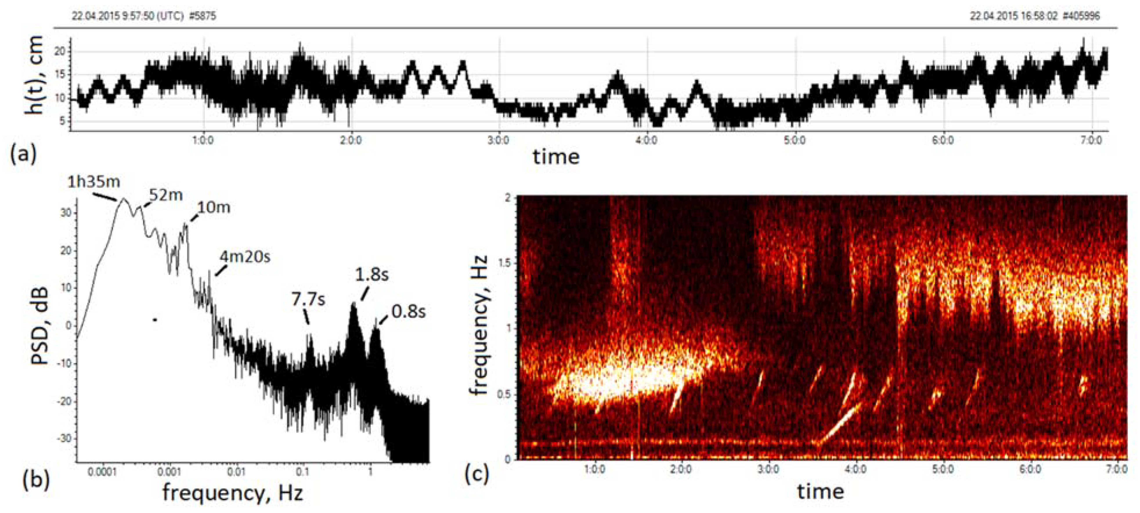
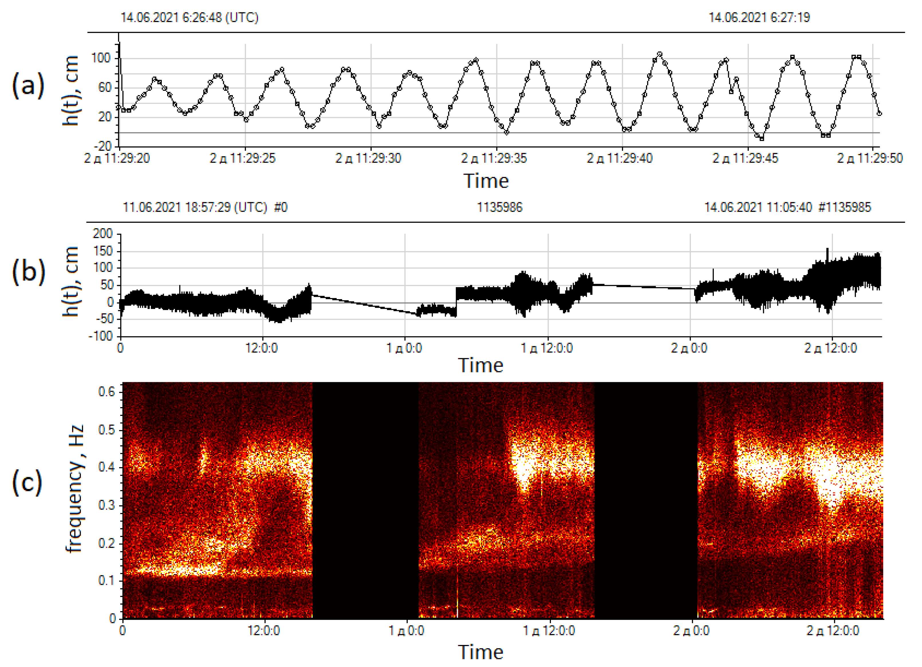
In addition to the frequency composition of the surface wave, it is possible to estimate the significant wave height (SWH) for different wave systems. Below is an explanation of the technology. Based on viewing the spectrogram, the time interval was determined, in which the wave system of interest to the user was visible and stationary. For example, for the swell in Figure 11c, it is logical to choose the first half of the first day. Figure 12a,b shows a three-hour recording of the h(t) signal from this area and its spectrogram. It is evident that the swell component, which corresponds to a continuous bright stripe in the lower part of the spectrogram, was stationary. In the Fourier spectrum of the h(t) signal, the leftmost peak corresponded to the swell waves, as shown in the upper half of Figure 12c. The blue curve shows a band-pass filter applied for frequency filtering of the swell component hf(t) from the total signal h(t). The spectrum shown in the lower half of Figure 12c confirmed that the filtration was correct. Figure 12d shows a 30-s fragment of the hf(t) signal. Using the downward zero-crossing algorithm [18], individual waves were selected from hf(t) (one of them is shaded in brown in Figure 12d); for each wave, two characteristics were determined—height (the difference between the maximum and minimum values) and duration (period). Figure 12e shows an OceanSP information window with the results of the statistical analysis of the extracted wave set. One of the statistics is SWH, the average height of 1/3 of the highest waves; in this case, SWH = 28 cm. In addition to statistics, the information window displays histograms of wave distribution by their heights and durations (periods).

The same analysis was performed to estimate the SWH of intense wind waves observed at the end of the third day of the study discussed above. SWH, in that case, was equal to 88 cm. Note that the described method can give overestimated SWH estimates if the frequency peak of the wave system of interest is observed in the spectrum against the background of powerful frequency components caused by noise or other wave systems close in frequency.

Experimental Study of One Simple Scheme for Obtaining Subpixel Resolution When Tracking Objects

On 11 June 2021, a small experimental study was carried out to practically investigate the possibility of achieving subpixel resolution when tracking objects. This problem is constantly in the focus of attention of specialists dealing with coastal video monitoring. Thus, in the work [19], it is considered in connection with the problem of the most accurate positioning of reference points, used for the georeferencing of video scenes, which must be observed continuously for several years. Under the influence of various factors, these points begin to shift, and it is important to track these changes with pixel accuracy, for example, with the accuracy $\mathsf{\Delta }{x}_{new}=0.2·\mathsf{\Delta }{x}_{old}$, where $\mathsf{\Delta }{x}_{old}$ is the pixel size in the plane of reference points. Rodriguez-Padilla [19] describes a simple and effective method based on image subpixel cross-correlation that has improved the accuracy of positioning of the reference points. In principle, almost all approaches are based on specially developed procedures for interpolating source images or video frames into more dense sampling grids. The task is to find such procedures that would minimize a selected quality criterion that is important for a particular field, taking into account additional restrictions. However, it can be assumed that simpler interpolation schemes, such as those used in CCTV cameras Digital Zoom mode, can also produce subpixel resolution when tracking very distant small objects.

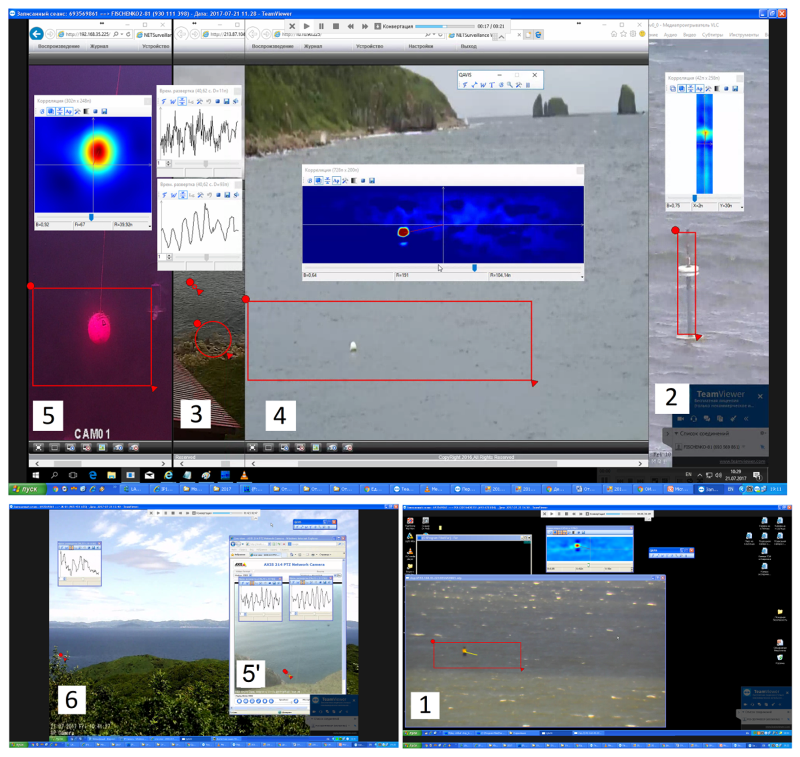
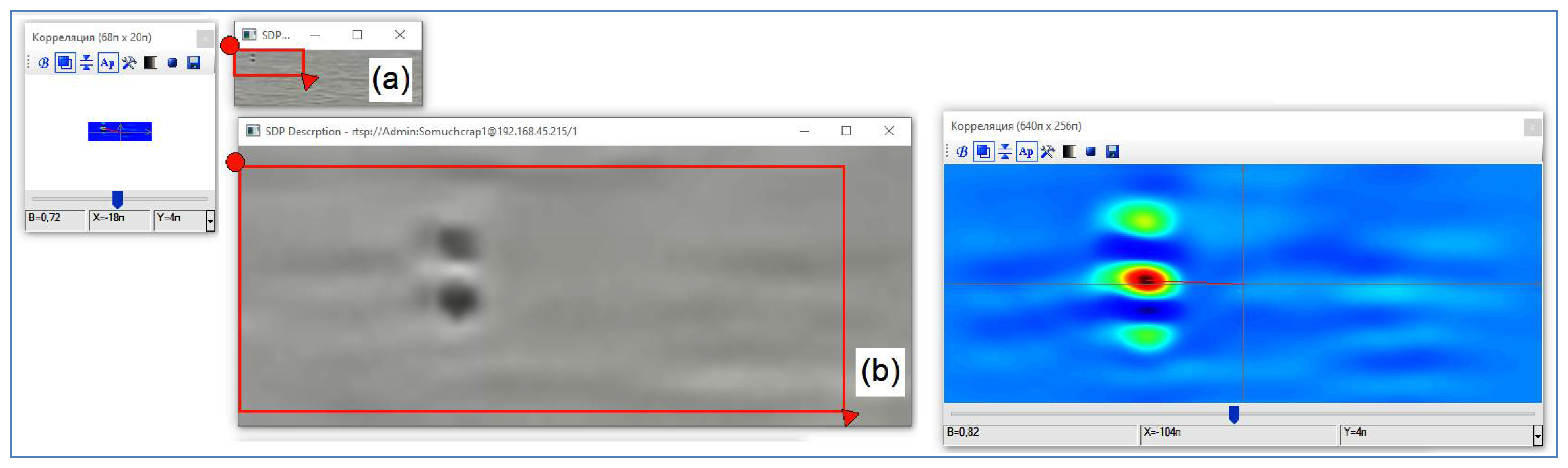
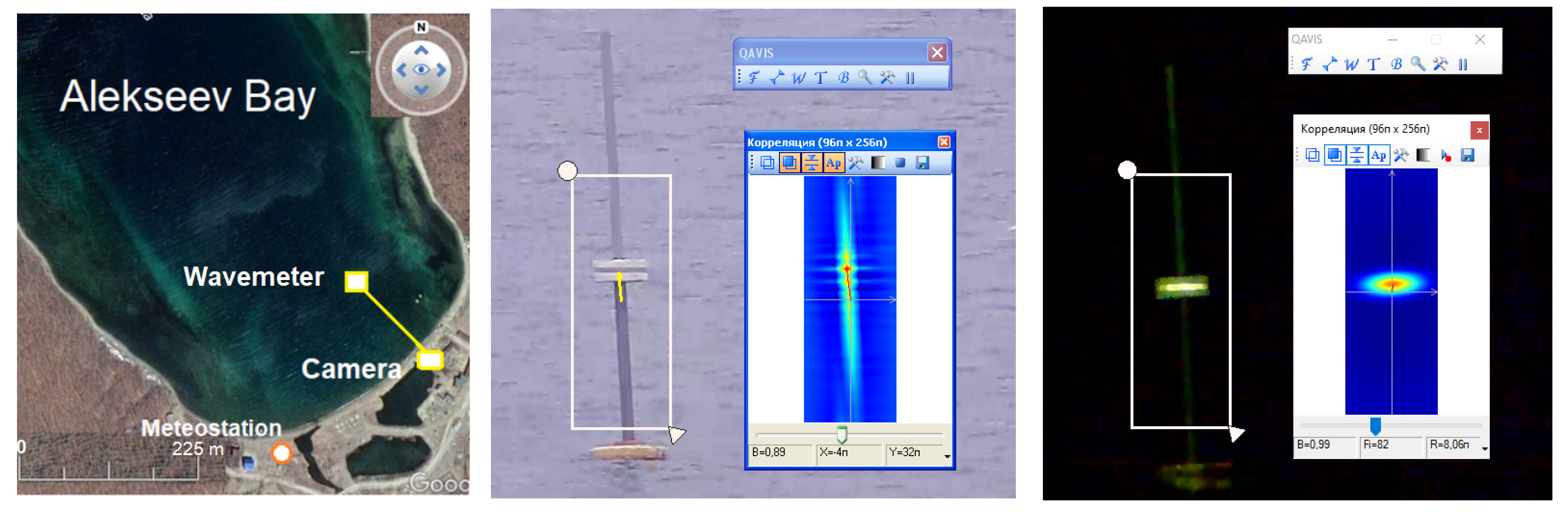
The following study was conducted to evaluate the subpixel resolution capabilities of bicubic interpolation using two PTZ cameras—OMNY 2030-IR and the previously described Hikvision DS-AELW. On 11 June 2021, simultaneously with Hikvision, an OMNY camera located on the roof of the institute streamed a navigational buoy scene with an optical zoom of 2.5×. The buoy looked like a very small object with a size of about 3 × 7 pixels; the height of one pixel in the observation plane of the buoy was approximately 43 cm. The streamings were carried out using the FFplay program simultaneously in two windows, the first—with the original resolution, the second—with 12-fold bicubic interpolation; the total zoom was 2.5 × 12 = 30×. Figure 13 shows the process of measuring the vertical movements of the buoy in both windows.

At the same time, the Hikvision camera streamed with the maximum optical zoom of 30×. The signal of vertical movements of the buoy, measured on it, can be considered the reference signal. The main goal was to find out whether bicubic interpolation leads to an increase in the accuracy of tracking the movements of the buoy, i.e., to the effect of subpixel resolution. Let the names of the received buoy movement signals be associated with the streamings: h1-OMNY (2.5×), h2-OMNY (2.5 × 12 = 30×), h3-Hikvision (30×). All three signals are measured in pixels. Another signal used in the study was the BHN seismic signal, synchronously recorded at Cape Schultz (94 km from the buoy). As mentioned above, the BHN signal is used to monitor the occurrence of swell entering the bay. The BHN signal is presented on integer conventional units (CU). For it convert to actual velocities signal it is necessary to use a scale factor of $4.54\times {10}^{-9} \mathrm{m}/\mathrm{s}$.

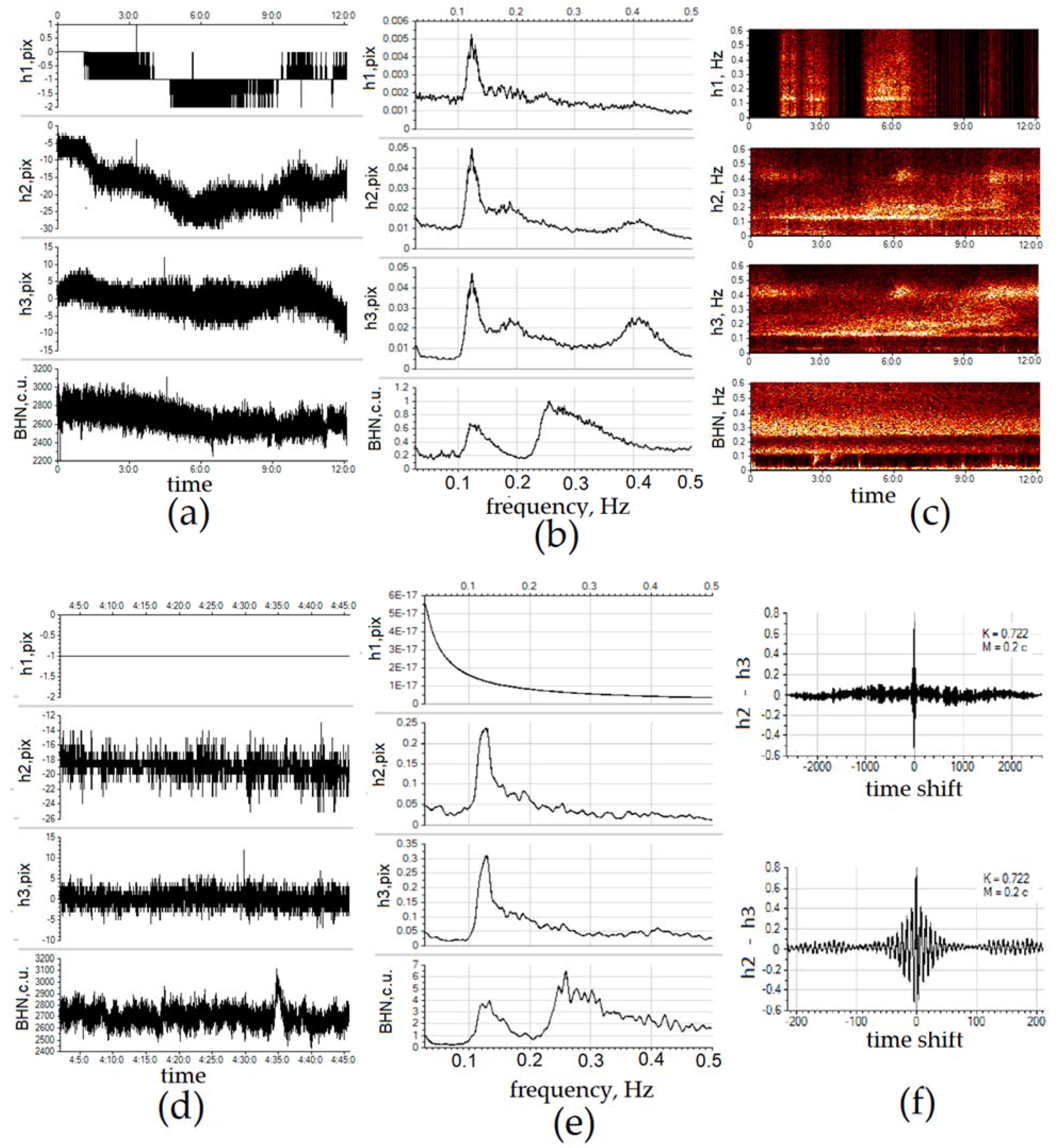
Figure 14 shows the results of the study. Figure 14a shows the waveforms of 12 h recordings of all channels. The h1 signal does not look much like ordinary signals, as it has only three gradations of the level. There are also long sections of constant zero values. The h2 signal, obtained using bicubic interpolation of the first stream, looks more like a signal with continuous values due to having more gradations of the level. In the spectra of three QAVIS signals h1, h2, h3 (see Figure 14b), a swell response with a period of about 8 s (0.13 Hz) is noticeable, which is confirmed in the spectrum of the BHN seismic signal. In the spectra of the interpolated and reference signals, h2 and h3, more wave systems with periods of 5.4 s (0.18 Hz) and 2.5 s (0.4 Hz) are synchronously manifested. The analysis of the spectrograms in Figure 14c further confirms the positive effect of bicubic interpolation use. The spectrogram of the non-interpolated signal h1 contains only two small sections with swell responses. The h2 spectrogram conveys the temporal dynamics of wave systems almost as well as the spectrogram of the reference signal h3. Figure 14d–f considers the unique case when there are no changes at all in the h1 signal for 44 min; the buoy does not shift by a single pixel in the field of view of the OMNY camera. At the same time, the movements of the buoy are recorded in the interpolated h2 signal; there is a peak in their spectrum at the swell frequency, the same as in the h3 and BHN spectra. In addition, the h2 signal is significantly correlated with the reference signal h3 (see Figure 14f).

Thus, a simple bicubic interpolation of a video fragment with a tracked marker can significantly improve the quality of tracking. Video streaming programs usually support the bicubic interpolation operation; many, IP cameras support the Digital Zoom with bicubic interpolation. This is important for the QAVIS-technology, since it will be possible to measure wave processes at significantly large distances in real time.

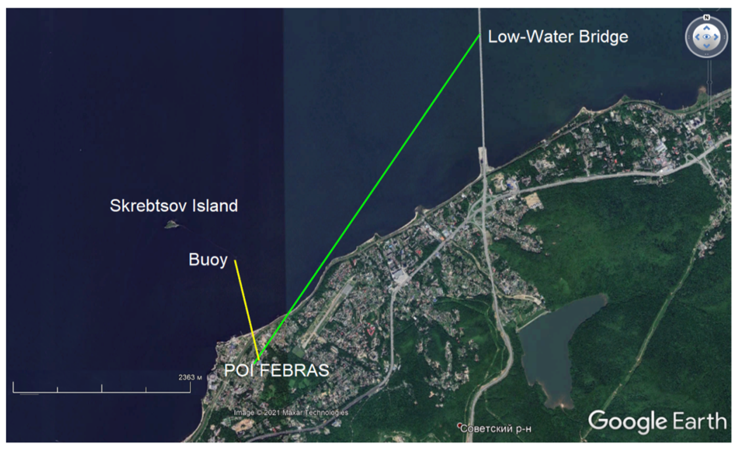
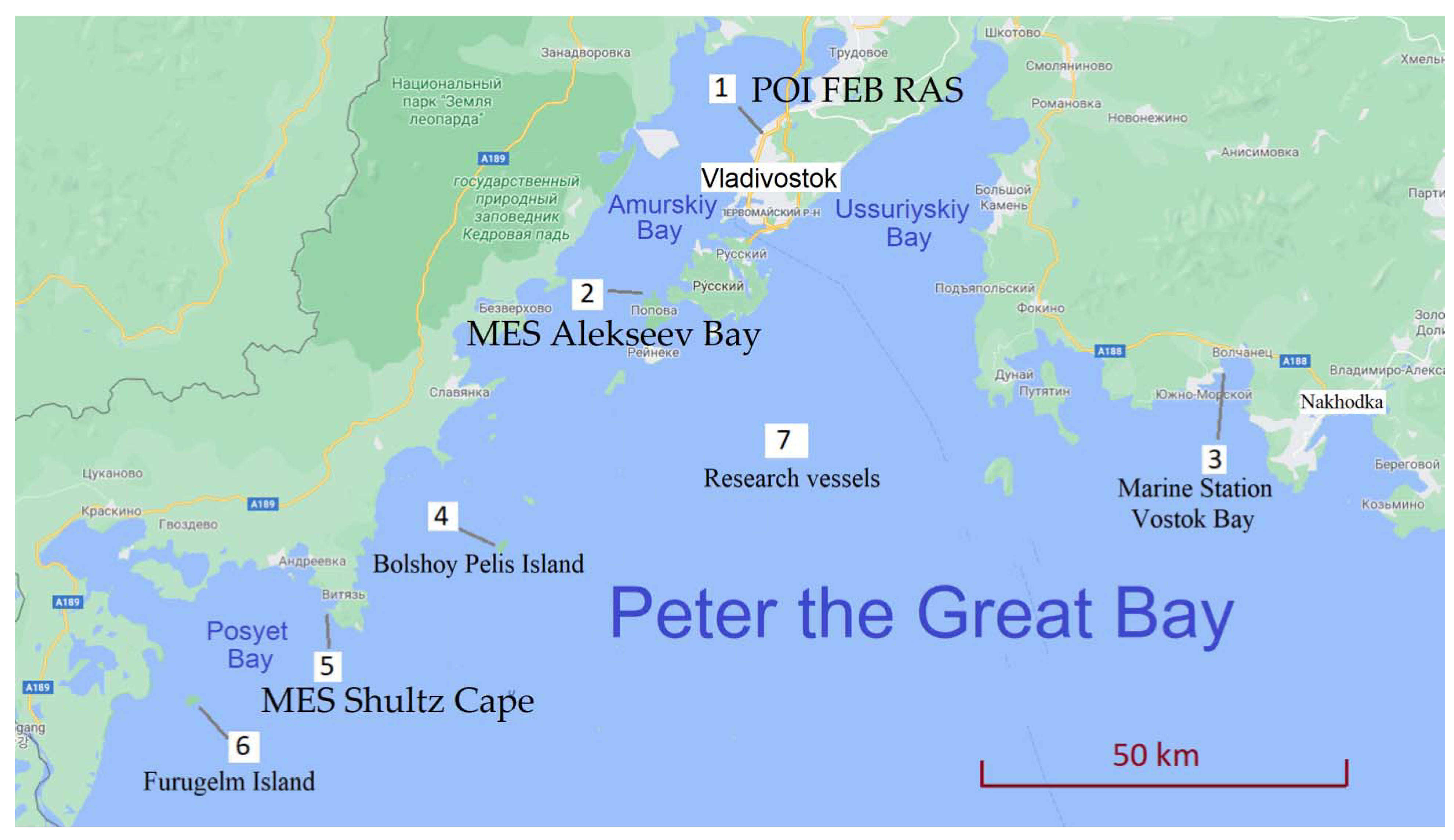
Let us return to the problem of studying the capabilities of the program for evaluating wave signals at ultra-long distances. In Figure 9, the green segment indicates the route from the OMNY PTZ camera on the roof of the POI FEB RAS building to the central spans of the low-water bridge over Amurskiy Bay (distance 5.4 km) (https://eng.gpsm.ru/activities/low-water-bridge-vladivostok/, accessed on 25 September 2021). From the autumn of 2020 to the present, several observation cycles have been performed to develop QAVIS-methods for estimating the parameters of sea processes at such large distances. 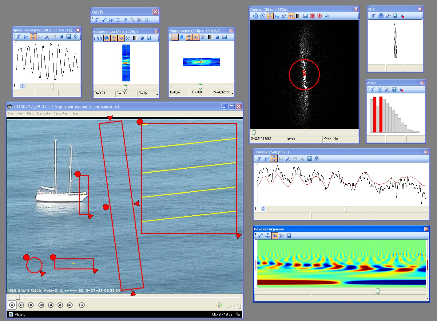Figure 15 shows the results of one of these studies.

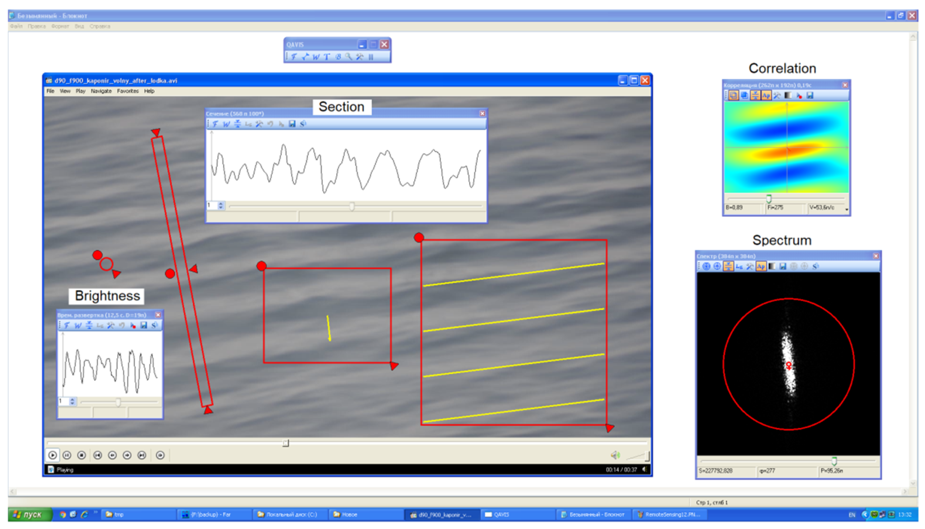
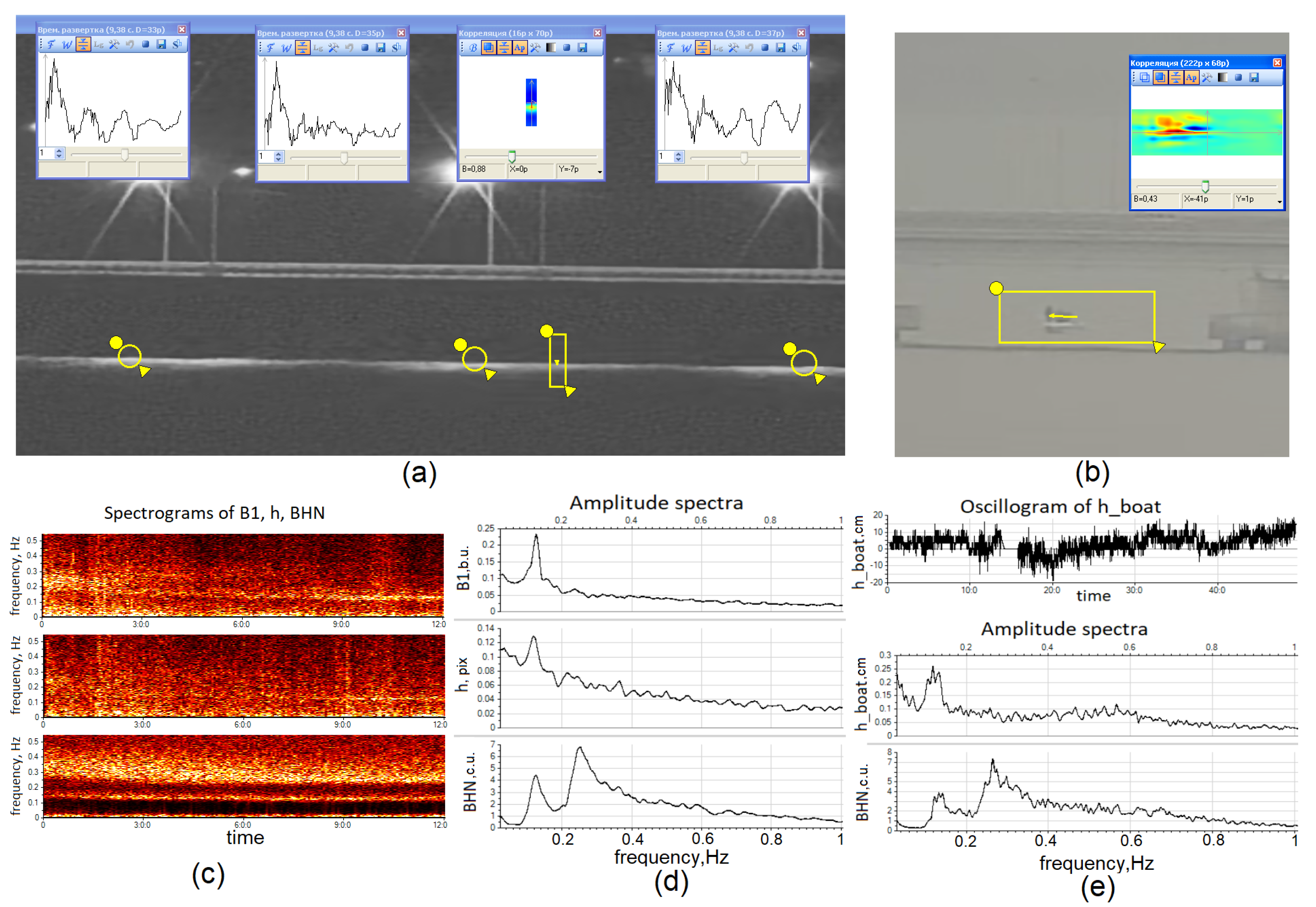
Figure 15a demonstrates the process of measuring fluctuations in the water of light spots from the bridge lights with instruments Brightness and Correlation. The measurements were carried out for 12 h during nighttime from 31 October to 1 November 2020. Figure 15c shows the spectrograms of signals B1 (brightness tool, left selector, measured in brightness units (b.u.) in the range from 0 to 255), h (correlation tool measured the vertical displacements in pixels of a strip of light on the water surface), BHN (a seismic signal, synchronously recorded at Cape Schultz, 98 km from the bridge). In the spectrograms of the “optical signals” near the end of the recording, light horizontal stripes are visible at a frequency of about 0.12 Hz. The same band is reproduced more clearly in the spectrogram of the BHN signal. Such frequency bands are characteristic of swell waves. In the spectra (Figure 15d) of 1-h fragments, the peaks corresponding to the swell periodicity of 8.3 s (frequency 0.12 Hz) are synchronously present for all three signals. Thus, the techniques of night measurements at very long distances tested in this example may well be applied to detect swell waves and describe their frequency properties.

Figure 15b,e demonstrates another small experiment, typical of the QAVIS technology. On the same day, 1 November, a fishing boat was accidentally discovered in one of the bridge spans on the main video broadcasts. In order not to overload the processing with a large number of measuring instruments, another video stream was launched on another computer; QAVIS was called to measure the movement of the boat bobbing on the waves (Figure 15b). Before the sailors left the camera’s field of view, it was possible to record a 49-min signal of the vertical movements of the boat h_boat. Figure 15e shows the waveform of the h_boat signal, its spectrum, and the spectrum of the BHN seismic signal at Cape Schultz. The spectra show synchronously low-frequency peaks of the same swell near 8.3 s. Taking into account the known height of the low-water bridge, the scale factor K = 3.66 cm/pix was calculated and applied. Then, the swell component was isolated using a bandpass filter, and its significant wave height SWH = 7.1 cm was estimated.

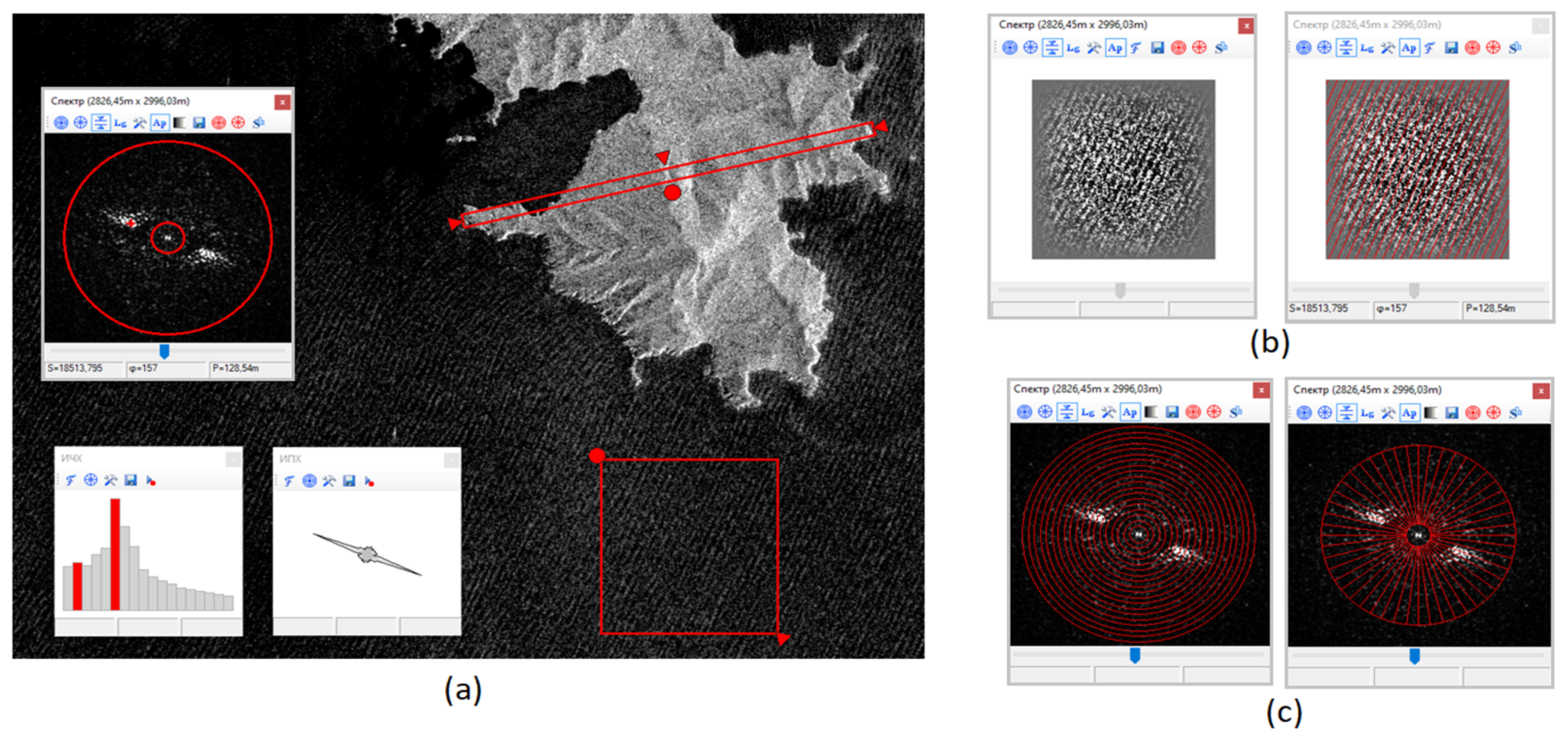
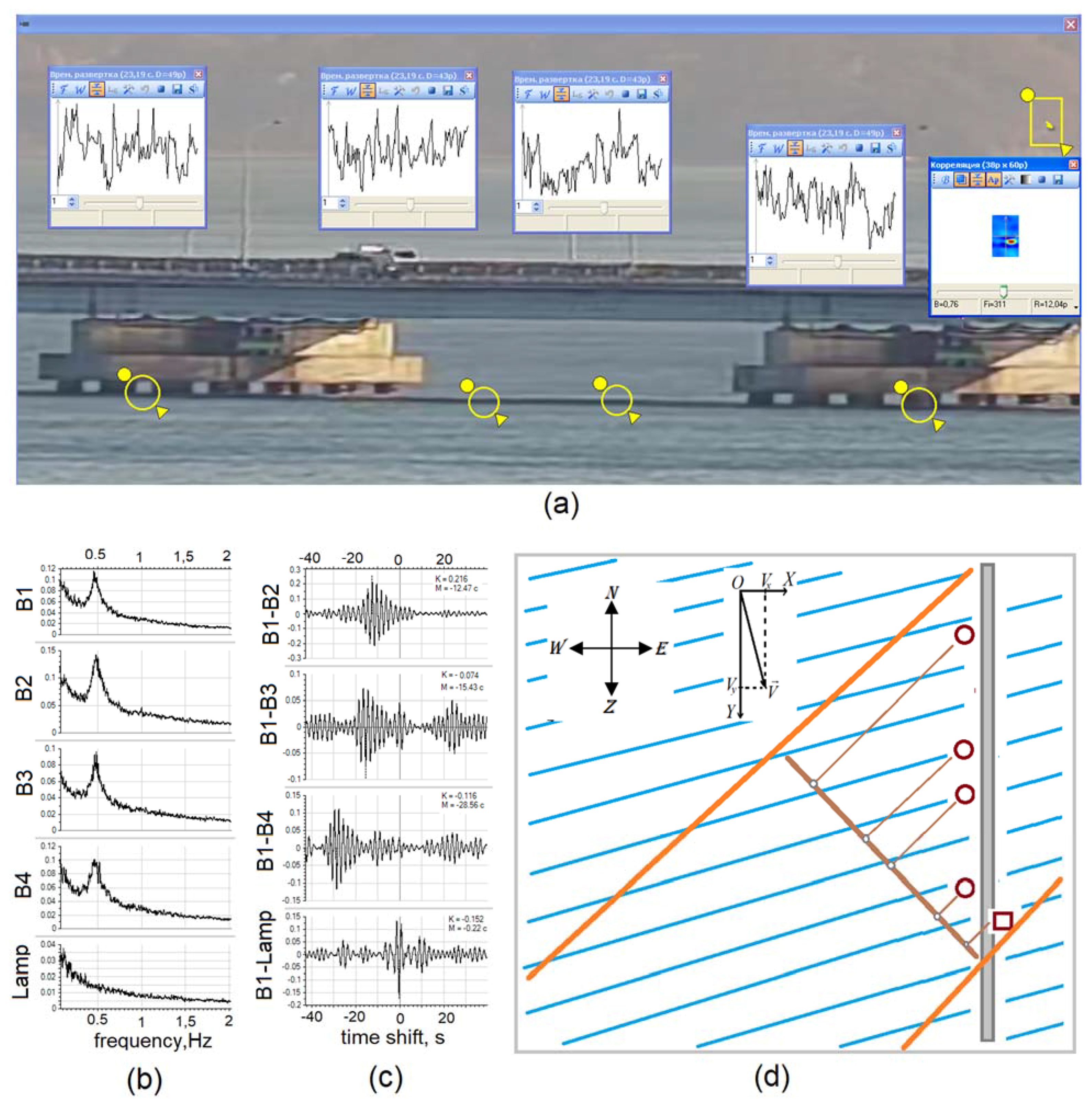
Figure 16 shows the results of observations near the low-water bridge on the night of 14–15 October 2020, in which wind waves with a period of 2.1 s were detected and described.

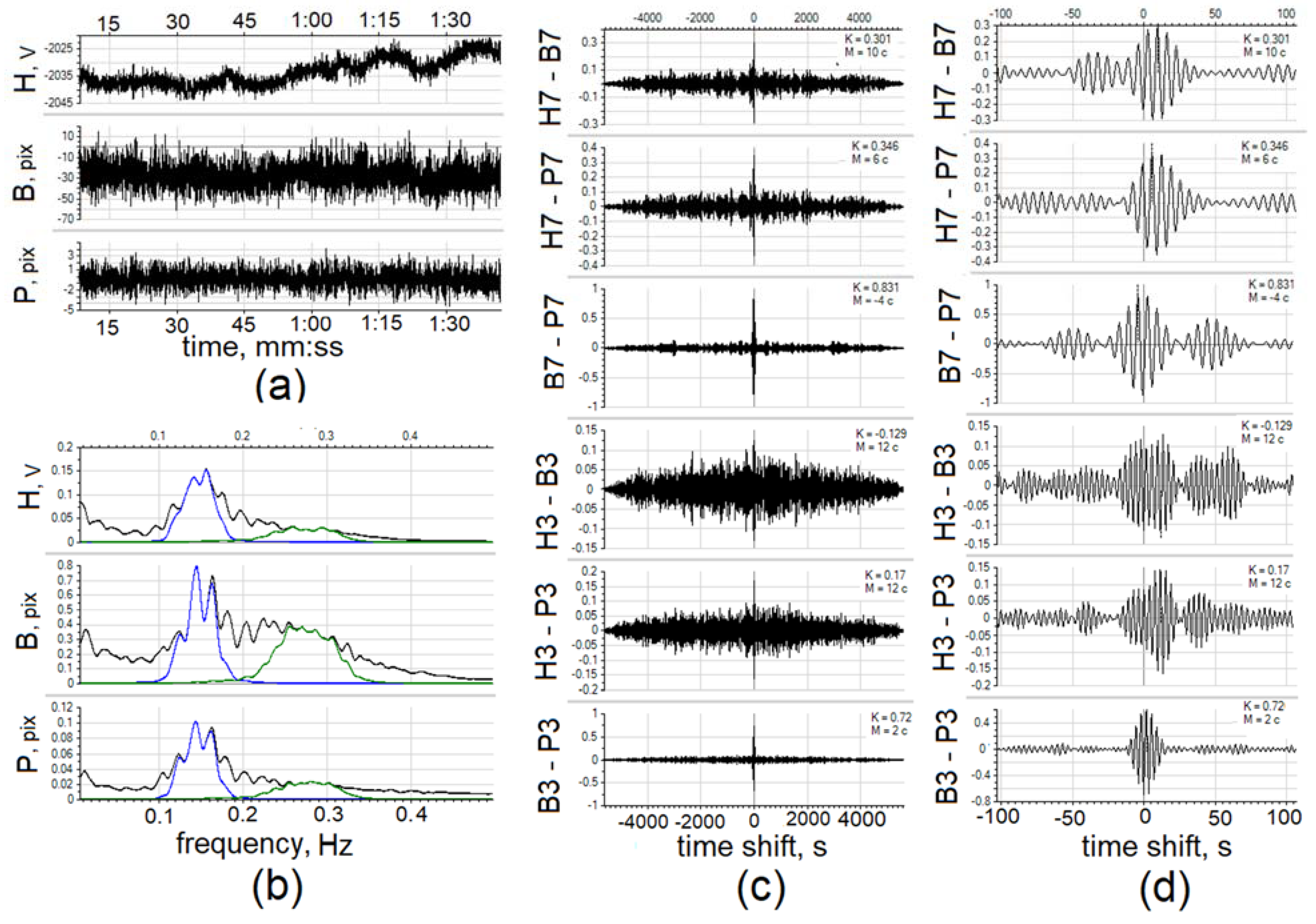
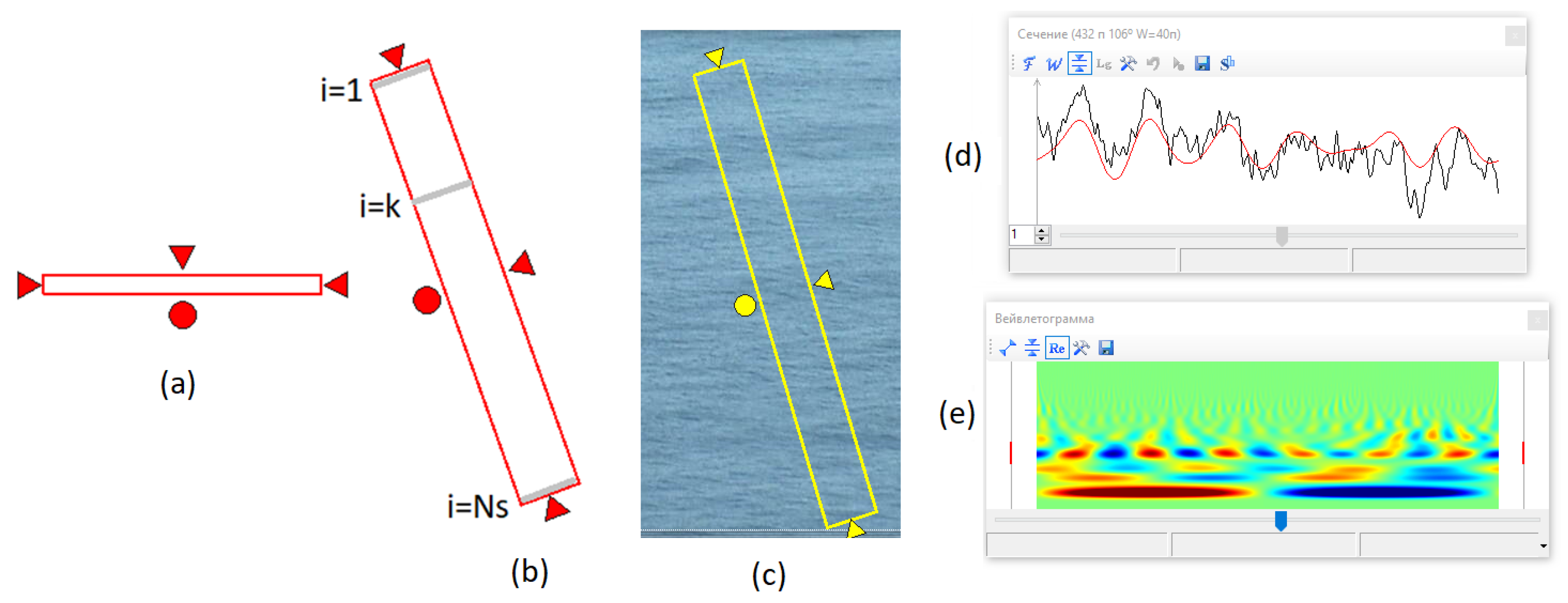
Figure 16a shows the measurement tools set-up that was used in nighttime measurements. Four round selectors of the brightness instrument measured the signals of fluctuations in the brightness of light spots on the water at night: B1, B2, B3, B4. The correlation tool (rectangular selector at the top right) measured the movement of a street lamp on a bridge. Figure 16b shows the Fourier spectra of two-hour signal records. In the spectra of all brightness signals, a peak corresponding to a period of 2.1 s is noticeable. There is no such peak in the movement of the street lamp signal.

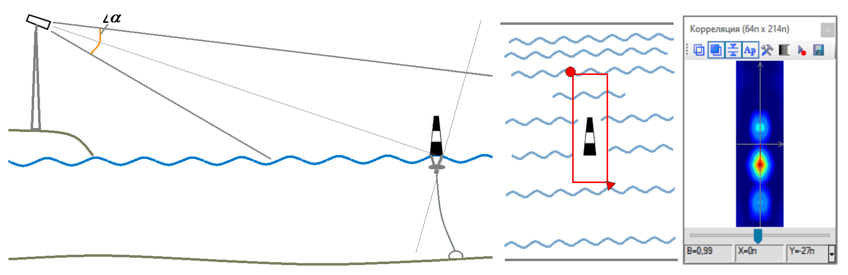
Then, the components of wind waves were extracted from all signals using a band-pass filter (the bandwidth is 0.4–0.6 Hz). Then, the correlation functions were calculated between the signal component B1 and the components of the remaining signals. In all correlation functions, the peaks of the correlation maxima were visually noticeable (see Figure 16c). In this case, the values of the maxima themselves were not large, from 0.08 to 0.23. It is noticeable on the graphs how the correlation maxima of the brightness signals successively move away from the point of zero shift with an increase in the distance between the measuring instruments. The values of time shifts between signals, determined by the program automatically according to the position of the maximum of the correlation module, were as follows: M12 = −12.47 s, M13 = −15.43 s, M14 = −28.56 s. The negative sign of the time delay means that the first signal is ahead of the second. The sequence of delays is logical if we take into account the uneven installation of the meters in Figure 16a.

A possible scenario for nighttime observations is presented on the schematic map shown in Figure 16d. The map shows the location of the bridge (gray vertical bar on the right), location of measuring instruments (brown circles) along the bridge, and conditional lines coming from the camera, limiting the field of observation of the scene to the left and right in Figure 16a, observation plane (brown line), orthogonal to the optical axis of the camera, the projection of the positions of the measuring instruments on the observation plane. The top left shows the wind rose. The direction of the bridge, and hence the line of placement of the meters along it, are oriented almost exactly along the “North-South” direction. This fact can be checked from Figure 9 and in the Google Earth service. The blue lines schematically represent wind waves moving from the direction of North-North-West. Usually, in October, north-westerly winds prevail over the Amur Bay. They could well have caused the wind waves shown in the diagram. The diagram also shows the velocity vector of the waves; its vertical component Vy can be estimated taking into account the known technical information about the dimensions of the bridge elements (https://eng.gpsm.ru/activities/low-water-bridge-vladivostok/, accessed on 25 September 2021). The distance D between the bridge supports is 63 m. Figure 16a shows that the distance between gauges 1 and 4 is slightly larger, D14 = 70 m. Thus, the projection of the wind waves velocity along the bridge can be estimated Vy = D14/M14 = 2.45 m/s.

The correlation between B1 and Lamp signals should be discussed. The correlation maximum is significant; it noticeably exceeds the average level of the surrounding correlations (see Figure 16c) but is reached at a very small time shift of 0.22 s, almost zero. When the distance between the meters is more than 70 m, the correlation with zero delay cannot be due to marine processes. The most likely cause is camera shake, which appears synchronously in the signals of all meters and therefore contributes to the correlation functions at zero time delay. With a strong jitter, situations are possible when the correlation of jitter components will exceed the correlation of real physical signals recorded by the meters. This can cause difficulties, and even errors, in the interpretation of observation results. In the previously considered case with the registration of swell waves near the bridge, significant peaks in the cross-correlation functions were observed for almost all pairs of signals. But only for two pairs of signals from closely spaced meters, these peaks were achieved with a nonzero delay. Apparently, at large distances, the correlation of real processes weakens, and the correlation of the jitter components begins to prevail.

Thus, in this section, it was shown that using QAVIS measuring techniques and OMNY 2030-IR class IP cameras, it is possible to detect swell and wind wave systems, and also to describe their frequency properties at distances of up to 5 km from a camera.

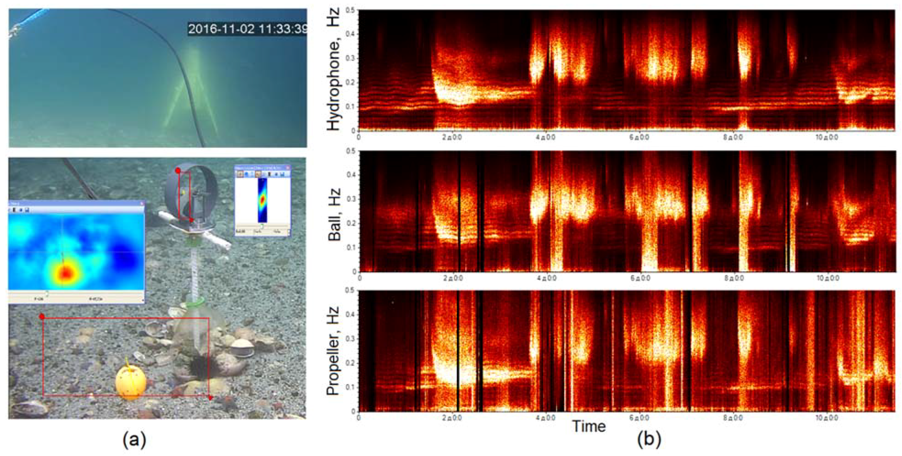
Strictly speaking, for wind waves, this statement is not supported by alternative field measurements. The seismic station at Cape Schultz does not register responses of wind waves in water areas remote from the Cape. The spectra and spectrograms of the buoy movement signal (Figure 14) contain powerful components in the range of 0.3–0.5 Hz, which usually reflect wind waves. However, the natural vibrations of the buoy structure may be manifested in the same frequency range. Therefore, it is advisable to conduct additional research using wave meters located next to the buoy. The fact of registration of wind waves near the low-water bridge (Figure 14) looks very reasonable. The data of all four wave meters are consistent with each other and satisfy one of the most realistic scenarios of the wave process for this part of Amur Bay. But even in this case, there were no data from alternative measuring systems.

3.2. Videowavemeters

Measurements of the wave signal h(t), based on tracking anchored marker objects (buoys, ships), contain an uncontrollable error associated with horizontal movements of the marker on the sea surface. They can make a small indefinite contribution to the vertical displacements of the object in the field of the video frame. Usually, horizontal movements are relatively slow and practically do not affect the height measurements of faster surface waves. However, such errors may be unacceptable for estimating the parameters of tidal and seiche fluctuations in sea level. Therefore, several methods have been tested, using specially placed structures in the sea, in which the horizontal movements of markers are limited.

One of the most successful designs of a stationary videowavemeter was first tested in 2014 in Alekseev Bay (point 2 in Figure 1). A six-meter-long pipe was rigidly driven into the seabed at a depth of about four meters. The distance from the shore was 100 m (110 m from the camera). A free-sliding light marker structure was mounted on its end, protruding above the water. The installation of the marker on the stand ensured its visibility in case of a significant wave. A reflective tape was glued on the marker, illuminated at night from the shore with a narrow beam LED projector, which provided the possibility of round-the-clock measurements. The measurement accuracy is determined by the linear size of one pixel 0.48 cm. The observations made it possible to describe several seiche periodicities of Alekseev Bay previously noted in the works of [20], in addition to describing surface wave systems. Figure 17 shows the Alekseev Bay on the Google Earth map and the process of measuring the wave signal in the Alekseev Bay during the day and at night, using a videowavemeter.

Figure 18 shows an example of analysis of a seven-hour recording of the wave signal h(t) from 22 April 2015. Figure 18a shows the waveform of the measured signal. Its Fourier spectrum (Figure 18b) shows peaks, corresponding to the periods: (1 h 35 m, 52 m, 10 m, 4 m 20 s)—typical of seiches, 7.7 s—typical of swells, 1.8 s—typical of wind waves, 0.8 s—typical of short wind waves (wavelength is 1 m or less). On the time-frequency spectrogram (Figure 18c), the time dynamic of the frequency composition of the wave is very clearly visible. At the bottom, a horizontal band is visible at low frequencies, corresponding to the swell wave; it is present throughout the entire recording and does not depend on local weather conditions. At the beginning of the spectrogram, a bright area corresponding to intense wind waves is visible for 2 h, obviously caused by a strong northwest wind in Amurskiy Bay. After the third hour of recording, the responses of short waves that occur during south wind begin to prevail in the spectrogram at the top. Earlier, it was repeatedly observed with the help of data from an automatic meteorological station that with a north-westerly wind, wind waves prevail with periods of 2–3 s, going towards the coast of the sea station. With a southerly wind, short waves prevail (with periods of 0.6–0.8 s). This wind blows into the sea from the coast and manages to form only short waves to the place where the wavemeter is installed (100 m from the coast, see Figure 17). Furthermore, relatively short inclined linear tracks are noticeable in the spectrogram—the responses of ship waves from ships passing by the Bay. The slope of the tracks is due to the dispersion of the wave packet coming from a vessel towards the wavemeter; the frequency of the recorded waves gradually increases (the period decreases). By the slope and duration of the tracks, the distance to the ship that caused the ship waves can be roughly estimated.

Thus, with the help of videowavemeters, it is possible to organize very high-quality observations of the entire spectrum of oscillatory movements of the sea surface, from short wind waves to seiche and tidal fluctuations.

During the winter months, many bights and bays of the Primorsky Krai freeze over, so the use of marker systems placed in the sea is not possible. However, it is possible to organize observation of the movements of markers installed on the ice surface. Since 2015, winter observations of vertical ice movements have been regularly carried out in Alekseev Bay using a summer videowavemeter camera. Some results of summer and winter observations are given in [21]. The main conclusion: practically all systems of sea-level fluctuations that are observed in the summer months are manifested in the signals of fluctuations of the ice surface, from seiche fluctuations of the bay itself (period 4 min 20 s) to tidal diurnal and semidiurnal fluctuations

It should be noted that, although the measurements of sea-level fluctuations using the videowavemeter are very consistent with the known experimental and model data [20], direct synchronous observations using alternative sea-level meters and surface waves were not done. Such observations will need to be carried out, first of all, to assess the accuracy of measuring the amplitude characteristics of various wave systems by the videowavemeter.

3.3. Synchronous Measurements of Hydrosphere Pressure Variations by a Laser Hydrophone, and of Underwater Currents Variations by Underwater Video Analysis with QAVIS

Three fixed underwater video surveillance cameras located in Alekseev Bay (point 2 in Figure 1) and Vityaz Bay (point 5 in Figure 1) were included in the general system of scientific video monitoring of Peter the Great Bay. The goal was to develop technologies for long-term continuous monitoring of the state of the underwater biodiversity in the bay [22]. In addition to solving biological problems, methods for estimating by video the parameters of underwater currents and surface waves were developed [23]. To assess the correctness of these methods, data from other underwater observations, carried out by the scientific groups of the Institute, were used.

Figure 19 shows the results of 12-day measurements carried out in Vityaz Bay from 15–27 November 2016, using a laser hydrophone and an underwater camera.

A laser hydrophone installed on the seabed measured variations in hydrosphere pressure in the frequency range of up to 1000 Hz. In the low-frequency part of its spectrum (0–0.5 Hz), sea-level fluctuations and wave processes on the sea surface were primarily manifested. The underwater camera was used to measure variations of underwater currents based on QAVIS-tracking of horizontal movements of artificial or natural marker objects. Both instruments were installed at a shallow depth, about 5 m from each other (see Figure 19a). QAVIS correlation tools were used to measure horizontal displacements of a tennis ball with small negative buoyancy (Ball) and rotation of the propeller blades (Propeller) under the influence of water mass movements. The main reason for these movements at such a shallow depth was wave processes on the sea surface, primarily swell and wind waves. Both meters evaluated the one-dimensional projections of the current vector variations. The optical axis of the camera was oriented orthogonally to the coastline towards the opposite coast. Therefore, the Ball signal measured the projection of currents along the coast of the bay. The rotation plane of the propeller blades was initially oriented orthogonal to the optical axis of the camera to estimate the velocity component of currents across the bay. However, at the beginning of observations, the propeller was turned 30–40 degrees, presumably by a spotted seal (Phoca largha). Before that, the largha was seen several times near the propeller on the video. Figure 19b shows the spectrograms of 12 daily recordings of all three signals. The band of analyzed frequencies is 0–0.5 Hz. The signal of variations in hydrosphere pressure will be called below as Hydrophone. The spectrograms are visually similar, all of them well and synchronously track the very complex, non-stationary dynamics of frequency composition of wave processes in the bay. Long horizontal tracks in the low-frequency part of the spectrogram represent swell; bright spots in the high-frequency part represent wind waves.

The purpose of these observations was to test the performance of both optical methods for measuring variations of underwater currents, using a ball and a propeller as markers. The technique with a ball tracks the frequency properties of surface waves better than with a propeller. Both methods are inferior to the hydrophone when estimating the parameters of the seiche vibrations of the bay. In general, the ability to use an underwater camera, in addition to its main biological tasks, for solving the problems of continuous monitoring of wave processes on the sea surface and underwater is very useful. The results of many scientific experiments conducted in Vityaz Bay significantly depend on the hydrodynamic conditions in the water layer thickness. Therefore, information about spectral composition and intensity of variations of underwater currents in different periods may be important for researchers doing such work. This information is also important for marine biologists in the context of accompanying video information about the state of marine biodiversity with information about the external conditions of its existence.

Another way to test the objectivity of underwater QAVIS measurement techniques is to check if there is a significant correlation between the swell and wind wave signal estimates recorded by QAVIS and the hydrophone. The correlation of the Ball and Propeller with each other would prove that both methods work and measure the same processes. Correlation with the hydrophone measurement would prove that processes caused by surface waves are being measured. The second case is more difficult because the hydrophone was located 10 m from the camera. In Vityaz Bay, a complex hydrological regime leads to instability of the directions of motion of wave systems relative to the hydrophone-camera axis. This would lead to the fact that the time delay between the arrival of waves to the first and second meters will be unstable; accordingly, the correlation maximum would be blurred during long-term observation.

The described effect was confirmed when studying the correlations in the above-described 12-day records of the Hydrophone, Ball, and Propeller signals. To analyze the correlation, a fragment of the record was selected, and its spectrum was calculated. The wave systems detected in it—swell waves and wind waves—were filtered. After that, the cross-correlation function was calculated for each wave system. If a visually noticeable sharp peak stood out in it, then the signals were recognized as correlated. The position of the peak determines the delay between the arrival of waves to the meters. Preliminary calculations confirmed that the Ball and Propeller signals are almost always correlated (the correlation coefficient K is between 0.6 and 0.9), and the time delay is close to zero. The correlation function between long (from several hours to several days) QAVIS-records and hydrophone records usually had a diffuse peak. The correlation function between short recordings (from half an hour to two hours) sometimes had sharp correlation peaks for the analyzed wave systems. Figure 20 shows an example of the analysis of correlations for a short recording—1.5 h long. OceanSP was configured to analyze swell waves and wind waves with periods 7 s and 3.5 s, respectively. Figure 20a shows oscillograms of the analyzed signals, and Figure 20b their spectra. The spectra of the filtered swell and wind waves are shown in blue and green. Figure 20d,e shows the correlation functions between signals H3, B3, P3, H7, B7, and P7. The letter in the designation identifies the measured signal, the number, and the main period of the analyzed wave system.

Figure 20c displays the correlation functions over the entire area of time shifts; such a representation is convenient for an expert to decide about the significance of the correlation between the pair of signals under consideration. If the peak noticeably exceeds the immediate environment, then it can be considered significant. In the considered case, significant correlations between the components of the Ball and Propeller signals are clear. The correlation coefficients at the maximum points are 0.86 for swell and 0.72 for wind waves, even though different projections of currents were measured. This fact proves that both QAVIS methods are workable and can be used to assess one-dimensional projections of underwater currents. The correlation peaks between the QAVIS signals and the hydrophone signal can also be considered significant. Moreover, they are sharp, which means that both wave systems were stable in direction and speed during the observation. Figure 20d shows the central part of the correlation functions. It can be used to visually determine whether the program’s estimate of the time delay (M) between signals is unambiguous. In the case under consideration, the decision on the time delay M = 12 s for the H3–B3 pair may be ambiguous, since there is almost the same peak with a shift of M = −2 s on the left. However, the same 12 s delay was obtained for the H3–P3 pair.

In general, the presented results of the analysis of the correlations of underwater QAVIS measurements and laser hydrophone data can be considered another argument in favor of using underwater measuring techniques. These measurements are certainly not very accurate and complete. They estimate only one projection of the speed of the water movement, and the signal of the propeller has few gradations in the rotational speed. Nevertheless, even in this form, the data obtained with their help correlate with the data of more accurate, but also more expensive devices. It is also clear that there are tasks where high accuracy in measuring the parameters of underwater currents is required. Qavis, in its current form, is not ready for such tasks. However, it could be useful at the stage of developing high-precision measuring systems based on streaming video analysis for organizing long-term continuous observations of underwater currents.

3.4. Observations of Light Marker Buoys, Comparison with Laser Hydrophone Data

In the video monitoring system of Peter the Great Bay, small marker buoys that fell into the view area of CCTV cameras were often used to quickly estimate the wave characteristics. They were usually installed by fishermen or scientists for their own purposes. As a rule, buoys were anchored and moved on the surface within a limited area. In Section 3.1, it was noted that uncontrolled horizontal movements of markers present a problem for QAVIS measurement of water surface level fluctuations h(t) based on tracking the vertical movements of a marker in the observation plane. This problem is especially critical for assessing the characteristics of sea-level fluctuations, like seiches, but less critical for assessing the properties of other wave processes (swell, wind, and ship waves) since, as a rule, their spectra are separated from the spectra of horizontal movements. Nevertheless, the question of how correct it is to apply the results of QAVIS observations of the vertical movements of marker buoys to describe the properties of sea waves requires additional research using alternative measurement techniques.

In the summer of 2018, a small comparative experiment was carried out at Cape Schulz using the laser hydrophone described in the previous section and a stationary TANTOS IP camera. The hydrophone was installed in Vityaz Bay 110 m from the shore at a depth of about 18 m. The camera was installed on the shore on the roof of a boat hangar; installation height approx. 4 m above sea level. A small white buoy, which marked the location of the hydrophone, was visible in the video as an object with a diameter of about 5 pixels (Figure 21a). Its actual diameter is 25 cm. The Digital Zoom mode with 4× magnification was used to improve the visibility of the buoy. The zoom was implemented in TANTOS using bilinear interpolation. Thus, the size of the pixel at the location of the buoy was 25/5/4 = 1.25 cm. Measurements of vertical movements of the buoy (Buoy) were taken using the QAVIS Correlation tool (Figure 21b) with a sampling rate of 5 Hz. The buoy signal was combined with the concurrent hydrophone measurements for analysis.

Figure 21c–f shows the results of the analysis of one of the recordings with a duration of 5 h. Figure 21c shows the waveforms of the Hydrophone and Buoy signals. In both, an increase in the level associated with the tidal process is noticeable. However, the signals differ significantly. This fact confirms the validity of the recommendation not to use such QAVIS meters for recording sea-level fluctuations. Figure 21d shows spectrograms of both signals. In the spectrogram of the Hydrophone signal in the low-frequency region, two bright horizontal stripes are noticeable, corresponding to the periodicities of 5.6 and 9.5 s. They most likely correspond to two swell systems that arrived at the bay. Above, up to a frequency of 1 Hz, there are no other features; the spectrogram is uniformly black. The spectrogram of the Buoy signal also clearly shows two horizontal bands at the same frequencies. In this case, the entire spectrogram contains noise that is characteristic of roughly quantized signals. In the high-frequency region, the spectrogram shows about ten tracks of waves from vessels passing in the bay.

The spectra of both signals in Figure 21e contain peaks corresponding to swell periods of 5.6 and 9.5 s. At the same time, no other spectral features appeared in the Buoy spectrum, which could be caused by the buoy design and its weight. Although the spectra are similar, the ratio of powers of the 5 and 9 s swells in them is different. The 5.6 s swell has greater power in the hydrophone signal, while the 9.5 s swell prevails in the buoy signal. In this case, the buoy movements more accurately convey the actual power ratio of the wave process. With the increasing installation depth of the hydrophone, it becomes less sensitive to the effects of short-period waves. In addition to discussing the visual similarity of the spectra, it is important to investigate how correlated the wave systems are that both instruments detect. For this purpose, the swell components with the main periods of 5.6 and 9.5 s have been extracted using a bandpass filter. In Figure 21e, for clarity, their spectra are superimposed on the original spectra (green—swell with a period of 5.6 s, blue—swell with a period of 9.5 s). Then cross-correlation functions were calculated between the Hydrophone and Buoy signal components, separately for each swell system. In both cases, large values of the maxima of the normalized correlations were observed (0.84 and 0.76, respectively). Both components of the swell in the measurement data of both instruments are significantly correlated.

The described example showed the prospects of using the QAVIS methods for measuring the movements of marker buoys for the rapid detection and description of the frequency properties of wave systems present in the water area. At a larger scale of the scene, the wave signals h(t) would be measured with greater accuracy, which is determined by the size of a pixel in the observation plane of the marker buoy. This will reduce the noise level in the spectra and spectrograms. It is worth expanding the research by conducting synchronous observations using several cameras with different optical magnifications, and by placing the hydrophone at a shallower depth, where it will record all wave systems without attenuation. However, the ability to quickly obtain information on the spectral composition of waves with the accuracy shown in Figure 21 can already be useful in research work.

There is, however, one significant limitation. High waves between a buoy and the camera can disrupt the buoy’s visibility. Therefore, if the camera is not installed high enough, the described technique will often not work.

4. Conclusions

The article presented a technology developed for the analysis of data of the scientific video monitoring system of Peter the Great Bay (the Sea of Japan/the East Sea). Its key element is the QAVIS computer program. It implements a set of tools for studying the spatial and temporal characteristics of wave processes in coastal waters, based on real-time processing of streaming video from coastal cameras. The article described the QAVIS tools and several measurement techniques, implemented on their basis.

Using the example with a synchronous registration of the arrival of a 9 s swell in the bay on a satellite image and in the records of the seismic station, the capabilities of QAVIS for studying wave structures on satellite images of the sea surface were demonstrated.

The possibilities of methods for measuring wave signals, based on tracking vertical movements of anchored marker objects at distances up to 5 km from a camera, were demonstrated. The limitations of these methods were noted; they are good at registering signals of wind waves and swells, but they are not effective for measuring seiche and tidal fluctuations at the sea level. The reason for this is the horizontal movements of markers on the water surface, which make an uncontrolled contribution to the vertical displacements of the marker on the video frame.

A comparative experiment was carried out, which proved that the preliminary bicubic interpolation of the scene with a marker object allows achieving subpixel resolution in the task of measuring wave signals based on tracking the movements of markers.

The results were presented, proving that the method of measuring wave signals, using stationary videowavemeters, is the most effective. It allows studying the entire spectrum of wave movements, from short wind waves, with characteristic periods of 0.5–0.8 s, to tidal daily and half-a-day fluctuations.

The paper presented the results of 12 days observations in Vityaz Bay using a laser hydrophone and an underwater camera installed at a depth of 5 m. It was shown that the frequency properties of the surface wave signals measured by a hydrophone and the signals of underwater currents measured by video tracking of the Ball and Propeller markers are very similar. In general, both optical markers track the responses of wind waves and swells well, but they are inferior to the hydrophone in tracking seiche fluctuations at the sea level.

In addition to those discussed in this article, there were many more examples of the joint use of QAVIS and other measurement techniques. It should be noted also that the QAVIS-technology is easy to use and can easily be applied to the study of sea processes in any coastal waters of the World Ocean, from which video is streamed to the Internet. For example, in [24], the results of measurements of seiche fluctuations in the port of Crotone (Italy), carried out with the help of QAVIS, are given. Comparison with the GLOSS data of the CR08 station (http://www.ioc-sealevelmonitoring.org/station.php?code=CR08, accessed on 25 September 2021) located 400 m from the CCTV camera confirmed the sufficiently high quality of QAVIS measurements.

References

1. Holman, R.A.; Guza, R.T. Measuring run-up on a natural beach. Coast. Eng. 1984, 8, 129–140. [Google Scholar] [CrossRef]
2. Holman, R.A.; Bowen, A.J. Longshore structure of infragravity wave motions. J. Geophys. Res. 1984, 89, 6446–6452. [Google Scholar] [CrossRef]
3. Holman, R.; Stanley, J. The history and technical capabilities of Argus. Coast. Eng. 2007, 54, 477–491. [Google Scholar] [CrossRef]
4. Stockdon, H.; Holman, R.A. Estimation of wave phase speed and nearshore bathymetry from video imagery. J. Geophys. Res. Space Phys. 2000, 105, 22015–22033. [Google Scholar] [CrossRef]
5. Holman, R.A.; Symonds, G.; Thornton, E.B.; Ranasinghe, R. Rip spacing and persistence on an embayed beach. J. Geophys. Res. Space Phys. 2006, 111, C01006. [Google Scholar] [CrossRef] [Green Version]
6. Chickadel, C.C.; Holman, R.A.; Freilich, M.H. An optical technique for the measurement of longshore currents. Geophys. Res. 2003, 108, 3364. [Google Scholar] [CrossRef] [Green Version]
7. Davidson, M.; Van Koningsveld, M.; de Kruif, A.; Rawson, J.; Holman, R.; Lamberti, A.; Medina, R.; Kroon, A.; Aarninkhof, S. The CoastView project: Developing video-derived Coastal State Indicators in support of coastal zone management. Coast. Eng. 2007, 54, 463–475. [Google Scholar] [CrossRef]
8. Fischenko, V.K.; Golik, A.V.; Subote, A.E.; Zatserkovniy, A.V.; Dubina, V.A. Scientific video monitoring system of the Peter the Great Bay (Japan sea). Geoinformatics 2011, 4, 30–41. (In Russian) [Google Scholar]
9. Longuet-Higgins, M.S. A theory of the Origin of Microseisms. Philos. Trans. R. Soc. Lond. Ser. Math. Phys. Sci. 1950, 243, 1–35. [Google Scholar]
10. Dolgikh, G.I.; Valentin, D.I.; Dolgikh, S.G.; Kovalev, S.N.; Koren, I.A.; Ovcharenko, V.V.; Fishchenko, V.K. Application of horizontally and vertically oriented strainmeters in geophysical studies of transitional zones. Izv Phys. Solid Earth 2002, 38, 686–689. (In Russian) [Google Scholar]
11. Dolgikh, G.I.; Budrin, S.S.; Dolgikh, S.G.; Zakurko, A.G.; Kosarev, O.V.; Ovcharenko, V.V.; Plotnikov, A.A.; Chupin, V.A.; Shvets, V.A.; Yakovenko, S.V. Complex spatially dispersed polygon in the far east for earth observations. Meas. Tech. 2016, 59, 252–255. (In Russian) [Google Scholar] [CrossRef]
12. Yakovenko, S.A.; Budrin, S.S.; Dolgikh, S.G.; Chupin, V.A.; Shvets, V.A. Hydrophysical laser-interference complex. St. Petersburg Polytech. Univ. J. Phys. Math. 2016, 2, 294–298. (In Russian) [Google Scholar]
13. Dolgikh, G.; Budrin, S.; Dolgikh, S.; Plotnikov, A. Supersensitive Detector of Hydrosphere Pressure Variations. Sensors 2020, 20, 6998. [Google Scholar] [CrossRef] [PubMed]
14. Addison, P.S. Wavelet transforms and the ECG: A review. Physiol. Meas. 2005, 26, R155–R199. [Google Scholar] [CrossRef] [Green Version]
15. Landau, L.D.; Lifshitz, E.M. Fluid Mechanics, Course of Theoretical Physics, 2nd ed.; Pergamon Press: Oxford, UK, 1987; Volume 6, ISBN 978-0-08-033932-0. [Google Scholar]
16. Lendaris, G.G.; Stanley, C.L. Diffraction Pattern Sampling for Automatic Pattern Recognition. Proc. IEEE 1970, 58, 198–216. [Google Scholar] [CrossRef]
17. Rabiner, L.R.; Gold, B. Theory and Application of Digital Signal Processing; Prentice-Hall: Englewood Cliffs, NJ, USA, 1975. [Google Scholar]
18. Mangor, K.; Drønen, N.K.; Kærgaard, K.H.; Kristensen, S. Shoreline Management Guidelines; DHI: Hørsholm, Denmark, 2016; pp. 37–40. [Google Scholar]
19. Rodriguez-Padilla, I.; Castelle, B.; Marieu, V.; Morichon, D. A Simple and Efficient Image Stabilization Method for Coastal Monitoring Video Systems. Remote Sens. 2019, 12, 70. [Google Scholar] [CrossRef] [Green Version]
20. Smirnov, S.V. On calculation of seiche oscillations of the middle part of Peter the Great Gulf. Numer. Anal. Appl. 2014, 17, 203–216. (In Russian) [Google Scholar] [CrossRef]
21. Fishchenko, V.K.; Dolgikh, G.; Zimin, P.S.; Subote, A.E. Some Results of Oceanological Video Monitoring. Dokl. Earth Sci. 2018, 482, 1244–1247. [Google Scholar] [CrossRef]
22. Fishchenko, V.K.; Zimin, P.S.; Zatserkovnyy, A.V.; Subote, A.E.; Golik, A.V.; Goncharova, A.A. Stationary systems for underwater video surveillance of coastal water areas. Underw. Investig. Robot. 2020, 1, 60–71. [Google Scholar] [CrossRef]
23. Fishchenko, V.K.; Zimin, P.S.; Golik, A.V.; Goncharova, A.A. Utilization of stationary underwater surveillance systems for the estimation of underwater currents and sea disturbance parameters. Underw. Investig. Robot. 2020, 2, 62–73. [Google Scholar] [CrossRef]
24. Dolgikh, G.; Fishchenko, V.K.; Goncharova, A.A. Potential for Recording of Waves and Sea Level Fluctuations in the World Ocean Coastal Areas by Internet Video Analysis. Dokl. Earth Sci. 2019, 488, 1264–1267. [Google Scholar] [CrossRef]
Figure 1. Locations of surface and underwater video surveillance camera installation (Google Map service used).
Jmse 09 01073 g001
Figure 2. Synchronous measurements in real time of wave signals and their assessments at 6 points in Peter the Great Bay: (5) Cape Schultz, an underwater camera in Vityaz Bay, horizontal displacements of the underwater marker under the action of fluid movements caused by surface waves is measured; (3) Vostok Bay, the sea surface brightness signal, modulated by the passing waves, and the brightness signal of the region of the wave ashore are measured; (4) Bolshoi Pelis island, the signal of vertical movements of the float on the sea surface is measured; (2) Alekseev Bay on Popov Island, the wave signal is measured on base a “videowavemeter”; (6) Furugelm Island, the brightness signal in the breaking zone of waves emerging on a small rocky island is measured; (5′) Cape Schultz, view towards the Sea of Japan, the signal of the sea surface brightness modulation by passing waves is measured; (1) roof of the POI FEB RAS, view of the Amurskiy Bay, the signal of vertical movements of the navigational buoy under the action of waves is measured.
Jmse 09 01073 g002
Figure 3. QAVIS Main Menu.
Jmse 09 01073 g003
Figure 4. Basic QAVIS tools. The red selectors of the Brightness, Transect, Correlation, and Spectrum tools are arranged in order from left to right. The current results of the tools are displayed in the corresponding information windows.
Jmse 09 01073 g004
Figure 5. Two methods of detecting a wave signal with Brightness instrument: (a) registration of the processes of swell waves breaking when they come ashore; (b) registration of apparent movements of the shore during video surveillance from a ship, standing at the pier.
Jmse 09 01073 g005
Figure 6. Transect tool: (a) basic selector; (b) stretched selector with a transect calculation scheme S ( i ) ,   i = 1 , N s ¯ ; (c) example of transect installation on a sea scene; (d) waveform of transect; (e) Waveletogram of transect.
Jmse 09 01073 g006
Figure 7. Spectrum tool. Analysis of the satellite (Sentinel-2) radar image, 25 September 2020 (Sentinel-Hub EO Browser used). (a) the image with selectors, the spectrum, IFC and ISC plots; (b) a fragment of source image without and with overlapping wavefronts; (c) IFC and ISC calculation schemes.
Jmse 09 01073 g007
Figure 8. Measurement of the wave signal h(t): the observation scheme of the marker object and the measurement scheme, based on video analysis.
Jmse 09 01073 g008
Figure 9. Measurements of waves at long distances in Amurskiy Bay: map of the area (Google Earth service used).
Jmse 09 01073 g009
Figure 10. Registration of buoy movements: Correlation tool, Hikvision camera, optical zoom 30×.
Jmse 09 01073 g010
Figure 11. Results of 3-day (11–13 June 2021) measurement of the wave signals in Amurskiy Bay, based on the buoy verticals movement tracking with the Hikvision camera: (a) waveform of a 30-s fragment of the wave signal; (b,c) waveform and spectrogram of the entire three-day signal, respectively.
Jmse 09 01073 g011
Figure 12. Methodology for calculating the significant wave height (SWH) implemented in OceanSP: (a) initial three-hour signal h(t); (b) its spectrogram, the swell response is a bright band in the low-frequency region; (c) at the top is the spectrum of the signal h(t) (black graph) and the frequency response of the band-pass (blue graph); at the bottom is the spectrum of the filtered signal hf(t); (d) signal fragment hf(t), one of the waves separated by the downward zero crossing algorithm is shaded in brown; (e) OceanSP information window with the results of statistical analysis of the set of selected waves.
Jmse 09 01073 g012
Figure 13. Recording of the buoy movements on two streams from the OMNY camera: (a) with optical zoom of 2.5×, (b) when using additional 12-fold bicubic interpolation.
Jmse 09 01073 g013
Figure 14. Results of the experimental study to investigate the possibility of using bicubic interpolation of a video stream for tracking the movements of anchored objects on the sea surface with the QAVIS program with subpixel accuracy. Oscillograms (a), spectra (b), spectrograms (c) of QAVIS signals h1, h2, h3, and seismic signal BHN, recording duration 12 h. Oscillograms (d) and spectra (e) of the same signals at a 44 min time interval, when the signal h1 was strictly constant. Correlation function between signals h2 and h3 over the entire interval of time shifts and on its central part (f).
Jmse 09 01073 g014
Figure 15. Night QAVIS-measurements of wave characteristics near the low-water bridge (a), daytime measurements of a fishing boat vibrations on the waves; (b), results of measurement analysis (ce).
Jmse 09 01073 g015
Figure 16. Registration of wind waves near the low-water bridge on 14–15 October 2020: (a) placement of meters on the video scene; (b) Fourier spectra of two-hour signal records; (c) mutual correlation functions between signals; (d) schematic map of the study.
Jmse 09 01073 g016
Figure 17. Videowavemeter in Alekseev Bay. Shown from left to right: its location (Google Map used); measuring process of wave signals in the daytime and at night, respectively.
Jmse 09 01073 g017
Figure 18. Analysis of the 7 h recording of the wave signal (22 April 2015, 09:57–16:58): (a) waveform, (b) spectrum, (c) spectrogram.
Jmse 09 01073 g018
Figure 19. Underwater observations in Vityaz Bay on 15–27 November 2016: (a) laser hydrophone and measuring markers Ball and Propeller on the bottom of the bay; (b) spectrograms of Hydrophone, Ball and Propeller signals.
Jmse 09 01073 g019
Figure 20. Analysis of correlations in the signals of a laser hydrophone (H) and underwater meters of variations in underwater currents, Ball (B) and Propeller (P): (a) oscillograms; (b) spectra (the spectra of 7-s swell and 3-s wind waves are shown in blue and green, respectively); (c) correlation functions between signals of different meters, separately for swell and wind waves; (d) the same correlation functions, but more detailed in the central region of time shifts. Signals B and P are measured in pixels, signal (H) is measured in units of electrical voltage (V) received at the output of the hydrophone. To convert the H signal to a scale of hydrospheric pressure variations, a scale factor of 105.1 Pa/V must be applied.
Jmse 09 01073 g020
Figure 21. Comparative observations of wave processes in Vityaz Bay (28 August 2018) using a laser hydrophone and QAVIS: (a) scene observed by the TANTOS camera; (b) measurement of vertical motions of the buoy with the QAVIS Correlation tool; (c) oscillograms of 5 h signal records; (d) their spectrograms; (e) Fourier spectra; (f) correlation functions between wave systems detected by both instruments (separately for swell with a period of 9.5 sec and swell with a period of 5.6 s).
Jmse 09 01073 g021
Publisher’s Note: MDPI stays neutral with regard to jurisdictional claims in published maps and institutional affiliations.