Article

Modelling the Impact of Climate Change on Coastal Flooding: Implications for Coastal Structures Design

by
Achilleas G. Samaras
1,* and
Theophanis V. Karambas
2
1
Department of Civil Engineering, Democritus University of Thrace, Kimmeria, PC 67 100 Xanthi, Greece
2
Department of Civil Engineering, Aristotle University of Thessaloniki, PC 54 124 Thessaloniki, Greece
*
Author to whom correspondence should be addressed.
J. Mar. Sci. Eng. 2021, 9(9), 1008; https://doi.org/10.3390/jmse9091008
Submission received: 20 July 2021 / Revised: 12 September 2021 / Accepted: 13 September 2021 / Published: 15 September 2021
(This article belongs to the Special Issue Modelling of Harbour and Coastal Structures)

Abstract

:
In the present work, the impact of climate change on coastal flooding is investigated through a set of interoperable models developed by the authors, following a modular modelling approach and adapting the modelling sequence to two separate objectives with respect to inundation over large-scale areas and coastal protection structures’ design. The modelling toolbox used includes a large-scale wave propagation model, a storm-induced circulation model, and an advanced nearshore wave propagation model based on the higher order Boussinesq-type equations, all of which are presented in detail. Model capabilities are validated and applications are made for projected scenarios of climate change-induced wave and storm surge events, simulating coastal flooding over the low-lying areas of a semi-enclosed bay and testing the effects of different structures on a typical sandy beach (both in northern Greece). This work is among the few in relevant literature that incorporate a fully non-linear wave model to a modelling system aimed at representing coastal flooding. Results highlight the capabilities of the presented modelling approach and set the basis for a comprehensive evaluation of the use of advanced modelling tools for the design of coastal protection and adaptation measures against future climatic pressures.

1. Introduction

Climate change is expected to have significant effects on the intensity and frequency of occurrence of extreme weather events, consequently affecting sea levels, circulation patterns, currents and waves in oceans and seas around the world [1,2,3,4]. Moving from the open sea to the densely populated coastal zones, more frequent storm surges and higher waves will be experienced through a number of impacts such as beach/dune erosion and inundation of low-lying areas [5,6]. Increased flooding risks are projected to have dire effects on socioeconomic aspects at regional and global levels [7,8,9,10,11], thus dictating the need for effectively designed coastal protection and adaptation measures [12,13].
Coastal flooding is attributed to the combined effect of tides, surges and waves acting over a broad range of scales in space and time. As scales change, so do the interactions and relative importance of the above physical processes, with their connection growing stronger in the nearshore. There, water levels caused by tides and storm surges, combined with wave setup and onshore wave propagation, can lead to the overtopping of coastal structures and the inundation of low-lying coastal areas. This interplay between waves and water levels dictates the characteristics of the models needed for the accurate representation of related processes, while scale issues allow the use of modular modelling approaches based on varying-complexity nesting schemes and the coupling of interoperable models.
The modelling perspective of the above has been investigated over the last couple of decades by various researchers. The storm surge inundation model presented by Hubert and McInnes [14] can be identified as setting a new paradigm in relevant literature, especially regarding the introduction of an inundation algorithm based on a novel wetting/ draining scheme (for further reading on this, [15] present a concise literature review of wet/dry interface treatments in free surface flows). Sharing the fundamental modular modelling approach mentioned above, the works of [16,17,18,19,20,21,22,23] cover many different realizations of modelling systems for the simulation of coastal flooding, using various models and coupling/nesting techniques. A general modelling flowchart would indicatively include moving downscale in space and time from operational oceanography models to large scale circulation and wave generation/propagation models for coastal areas, and then to high resolution wave and hydrodynamics models in the nearshore, where wave–structure interactions and coastal inundation would be simulated. This general scheme does not exclude adding/removing simulation steps to its lower- and/or higher-resolution ends, or modifying internal model coupling, as these choices depend on data availability and the overall modelling objective. For example, if the modelling objective includes the study of climatic pressures per se, simulation steps should be added to the lower-resolution end of the aforementioned modelling flowchart in order to include a Regional Climate Model (RCM; one additional step) or a Regional Climate Model and a Global Climate Model as well (RCM + GCM; two additional steps).
Regarding the effect of coastal protection and its integration to a coastal flooding modelling system, one would have to start from the fact that the phenomenon itself is directly associated to the wave energy acting on beaches. Accordingly, the presence of coastal structures in the nearshore can significantly reduce flooding potential by reducing the wave energy reaching the shore, making such interventions a suitable countermeasure against storm-induced flooding in present and future climates. Key to the above is the transmissivity of the structure, i.e., the amount of energy transmitted over and/or through it, typically expressed in the form of a transmission coefficient Kt = Ht/Hi [24], where Hi and Ht are the incident and transmitted wave heights, respectively.
Among the various available options, Low-Crested Structures (LCS) are probably the most widespread technical interventions installed for the protection of natural and artificial beaches worldwide. As such, wave transmission behind them has been extensively studied over the years. Relevant works rely on experimental datasets for the derivation of empirical formulae for Kt through various approaches, others validate or seek to extend existent formulae through experimental/numerical investigations [25,26,27,28], while an emerging research field combines data analysis with Artificial Neural Network (ANN) techniques in order to provide tools able to predict wave–structure interactions [29,30]. Regarding specifically design formulae, reference should be made to: the fundamental works of [31,32]; the work of [33], who proposed a novel formulation using as basis the theoretical treating of the physical phenomena that govern wave transmission (i.e., breaking/overtopping/energy transfer); the work of [34], who proposed a formulation based on the summation of wave energy transmitted over and through LCS (following [35] and [36], respectively), as well as the update of this last formulation by [37].
This work presents the authors’ view, interpretation and implementation of a modelling system that would integrate the above aspects for practical coastal engineering applications. In the following, the impact of climate change on coastal flooding is estimated on the basis of a modular modelling approach, using three models developed by the authors and adapting the modelling sequence to two separate objectives with respect to inundation over large scale/regional areas and to coastal protection structures’ design. In Section 2, the modelling approach and theoretical background of the models are presented in detail. In Section 3, the capabilities of the numerical model at the higher-resolution end of the modelling sequence, i.e., an advanced model based on the solution of the higher-order Boussinesq-type equations, are validated through comparison with the experimental data by Roeber et al. [38] (coastal flooding) and with the formulation of Goda and Ahrens [34] (wave transmission at coastal structures). In Section 4, the rationale and setup of model applications for the two objectives described above is presented. Model results are presented and discussed in Section 5, while Section 6 presents the conclusions drawn from this work.

2. Model Description

Following the rationale described in Section 1, the present work retains the viewpoint of a modular modelling approach in order to simulate storm-induced coastal flooding. The modelling toolbox used includes a large-scale wave propagation model (WAVE_LS), a storm-induced circulation model (SICIR) and an advanced nearshore wave propagation model (WAVE_BQ). Based on the analysis of the interplay between waves and water levels at different scales, the modelling sequence is adapted to fit two separate objectives. The first one, aiming at simulating flooding over large/regional coastal areas, uses WAVE_LS and SICIR. In this, WAVE_LS provides the components of the radiation stress tensor to SICIR which is afterwards used to simulate coastal flooding. The second one, aiming at investigating the effect of the presence of coastal structures in the above context, uses WAVE_BQ as well. In this, SICIR results are used as offshore boundary conditions for WAVE_BQ, which is used to simulate wave overtopping and transmission behind the structures, and wave runup on beaches.

2.1. The Large-Scale Wave Propagation Model (WAVE_LS)

WAVE_LS is based on the directional wave energy balance equation [39,40]:
E t + c x E x + c y E y + c θ E θ = D
where E(f,θ|x,y,t) is the spectral density of frequency f and direction θ at a point (x,y) and time t; and cx, cy, cθ are the x, y, θ components of the group velocity cg, respectively, according to:
c x = c g sin θ c x = c g cos θ c θ = c g c ( cos θ c x sin θ c y )
In Equation (2), c is the wave celerity. In Equation (1), D is the dissipation of wave energy expressed as:
D = 1 4 Q b f ρ g H m 2
where Hm is the maximum wave height according to [41]; ρ is the water density; and Qb is the probability of a wave breaking at a certain depth, expressed as (1 − Qb)/(lnQb) = (Hrms/Hm)2 according to [42], where Hrms is the root-mean-square wave height. Wave diffraction is incorporated to the model by replacing cx, cy and cθ with Cx, Cy and Cθ according to [40]:
C x = c g sin θ ( 1 + δ ) C x = c g cos θ ( 1 + δ ) C θ = c g c ( cos θ c x + sin θ c y ) 1 + δ + 1 2 1 + δ c g ( cos θ δ x + sin θ δ y )
where κ is the wave number and δ is expressed as:
δ = . ( c c g E ) κ 2 c c g E
The model is capable of simulating wave propagation in large coastal areas with complicated bathymetries, describing the phenomena of refraction, bottom diffraction and breaking. The numerical solution of Equation (1) is based on an implicit finite difference scheme and the model’s output includes the four components of the radiation stress tensor (Sxx, Syy, Sxy = Syx), calculated by the well-known expressions valid for progressive waves, as in [43].

2.2. The Storm-Induced Circulation Model (SICIR)

The storm-induced circulation model is based on the depth-averaged wind-induced circulation equations, following [44]:
ζ ¯ t + ( U h ) x + ( V h ) y = 0
U t + U U x + V U y + g ζ ¯ x = 1 ρ h ( S x x x + S x y y ) + 1 h x ( ν h h U x ) + 1 h y ( ν h h U y ) + f c V + τ s x ρ h τ b x ρ h
V t + U V x + V V y + g ζ ¯ y = 1 ρ h ( S x y x + S y y y ) + 1 h x ( ν h h V x ) + 1 h y ( ν h h V y ) f c U + τ s y ρ h τ b y ρ h
where ζ ¯ is the water surface elevation above the mean water level; d is the still water depth; h is the total water depth ( h = d + ζ ¯ ); U, V are the depth-averaged velocity components along the x- and y- directions respectively; g is the gravitational acceleration; νh is the horizontal eddy viscosity coefficient and fc is the Coriolis coefficient. The terms τsx, τsy are the shear stress components at the water surface along the x- and y- directions respectively, which represent the vertical boundary condition, expressed as:
τ s x = ρ k W x W x 2 + W y 2
τ s y = ρ k W y W x 2 + W y 2
where k is the surface friction coefficient (in kg/m3, typically of the order of 10−6; here we assume k = 10−6 ÷ 3∙10−6), and Wx, Wy are the wind speed components along the x- and y- directions (in m/s, at 10 m above sea level) respectively. The bed friction terms (τbx, τby) are calculated based on the formulae proposed by [45]:
τ b x = 1 2 ρ f b σ T 2 G b x
τ b y = 1 2 ρ f b σ T 2 G b y
G b x = U σ T [ 1.16 2 + ( | U | σ T ) 2 ] 0.5
G b y = V σ T [ 1.16 2 + ( | U | σ T ) 2 ] 0.5
where fb is the bottom friction factor, σT is the standard deviation of the oscillatory horizontal velocity, and |U| = (U2 + V2)0.5. The horizontal eddy viscosity coefficient is expressed by the well-known Smagorinsky model, used for the representation of the damping by eddies smaller than the computational grid size, as:
ν h = 2 [ ( U x ) 2 + ( V y ) 2 + 1 2 ( U y + V x ) 2 ] 1 / 2
where is the mixing length, approximated as equal to half the grid cell size dx [46].
Differential Equations (6)–(8) are approximated by finite difference equations according to the explicit scheme developed by [44]. Finally, regarding coastal inundation, the process is simulated using the “dry bed” boundary condition which, according to [47], can be written as the following set of pairs of conditions for any given grid point (i,j):
if   ( d + ζ ) i , j > h c r   and   ( d + ζ ) i 1 , j h c r   and   U i , j > 0 U i , j = 0 if   ( d + ζ ) i , j > h c r   and   ( d + ζ ) i , j 1 h c r   and   V i , j > 0 V i , j = 0 if   ( d + ζ ) i , j h c r   and   ( d + ζ ) i 1 , j h c r   U i , j = 0 if   ( d + ζ ) i , j h c r   and   ( d + ζ ) i , j 1 h c r   V i , j = 0 if   ( d + ζ ) i , j h c r   and   ( d + ζ ) i 1 , j > h c r   and   U i , j < 0 U i , j = 0 if   ( d + ζ ) i , j h c r   and   ( d + ζ ) i , j 1 > h c r   and   V i , j < 0 V i , j = 0
where hcr is a terminal depth below which drying is assumed to occur (here this depth is set to hcr = 0.001 m).

2.3. The Advanced Nearshore Wave Propagation Model (WAVE_BQ)

Over the years, the classical Boussinesq equations have been extended by incorporating higher order non-linear terms, which can describe better the propagation of highly nonlinear waves in the shoaling zone. Nowadays, models based on Boussinesq-type equations (BTEs) are widely used to simulate waves transforming in the nearshore—up to the swash zone—and their interactions with various types of coastal protection. Exemplary reference is made to the recent works of [48,49,50,51,52,53], with [54] presenting a novel meshless numerical scheme for the solution of BTEs. A thorough overview of Boussinesq-type models can be found in [55].
WAVE_BQ is based on the higher order Boussinesq-type equations for breaking and nonbreaking waves as expressed in equations:
ζ t + ( h U ) = 0
U t + 1 h M u 1 h U ( U h ) + g ζ + G = 1 2 h [ ( d U t ) ] 1 6 h 2 [ U t ] + 1 30 d 2 [ ( U t + g ζ ) ] + 1 30 [ ( d 2 U t + g d 2 ζ ) ] d ( δ U ) t - τ b h + E
where Mu is defined as:
M u = ( d + ζ ) u o 2 + δ ( c 2 u o 2 )
and G as:
G = 1 3 { d 2 [ ( U ) 2 U 2 U 1 10 2 ( U U ) ] } 1 2 ζ [ ( d U t ) ]
where ζ is the wave surface elevation; the subscript “t” denotes differentiation with respect to time; U is the horizontal velocity vector U = (U,V); τb = (τbx, τby) is calculated from Equations (11) and (12), with the wave-current bottom friction factor calculated as in [56]; δ is the roller thickness, determined geometrically according to [57]; E is the eddy viscosity term, calculated according to [58]; and uo is the bottom velocity vector uo = (uo, vo), with uo and vo being the instantaneous bottom velocities along the x- and y- directions respectively. Following [56], wave breaking is initiated using breaking angle φb = 30°, which then gradually changes to its terminal value φb = 10°.
The presented set of BTEs is accurate to the third order O(ε2,εσ24) [59] and their numerical solution is based on the accurate higher-order numerical scheme of [60]. Coastal inundation is simulated as in SICIR (see Section 2.2, Equation (16) and [47]). The model is capable of simulating the phenomena of shoaling, refraction, breaking, diffraction, reflection and wave-structure interaction, as well as nonlinear wave-wave interaction. Regarding model capabilities in simulating the non-linear evolution of unidirectional or multidirectional wave fields in the nearshore, one can refer to [61] (see also [62] on the issue); regarding wave-structure interaction and energy transmission, one can refer to [63]. Further details on the model and its implementation to diverse coastal engineering applications can be found in [56,64,65].

3. Model Validation

3.1. Coastal Flooding

The capability of the presented advanced nearshore wave propagation model in the representation of coastal flooding is validated through the comparison with the two-dimensional (cross-shore) experimental data by [38]. Roeber et al. [38] tested wave transformation over idealized fringing reefs, carrying out a series of experiments in two flumes at the O.H. Hinsdale Wave Research Laboratory of Oregon State University. The first flume was 48.8 m long, 2.16 m wide and 2.1 m high; the second flume was 104.0 m long, 3.66 m wide and 4.57 m high with a reef crest. Both flumes were equipped with piston-type wavemakers for wave generation and resistance wave gauges for free surface measurement.
The experimental setup in the first flume included a steep 1:5 slope starting at x = 17.0 m, followed by a reef flat up to the flume’s rigid wall at x = 45.0 m (x being the direction along the flume). The test in this flume regarded a steep solitary wave of A = 0.5 m height and a water depth of d = 1.0 m, resulting in A/d = 0.5 and an initially dry reef flat. The discretization steps used in model (WAVE_BQ) runs were dx = 0.05 m in space and dt = 0.0025 s in time. Figure 1 shows the comparison between measurements and model results for this test, as a series of snapshots of surface profile evolution. Measured and computed data are in very good agreement at all transformation stages. The model successfully captures the wave’s skewness as it propagates across the toe of the slope, the formation of its steep front over the steep slope, and its eventual flow transition from sub- to super-critical as it surges over the reef flat.
The experimental setup in the second flume included a fore reef slope of 1:12 starting at x = 25.9 m, a 0.2 m reef crest and a reef flat behind it up to the flume’s rigid wall at x = 83.7 m (x being the direction along the flume). The test in this flume regarded a steep solitary wave of A = 0.75 m height and a water depth of d = 2.5 m (A/d = 0.3), initially exposing the aforementioned reef crest by 0.06 m and submerging the reef flat with 0.14 m of water. The discretization steps used in model (WAVE_BQ) runs were, again, dx = 0.05 m in space and dt = 0.0025 s in time. Figure 2 shows the comparison between measurements and model results for this test, as a series of snapshots of surface profile evolution. Again, as for the first test, measured and computed data are in very good agreement at all transformation stages. The model successfully captures wave shoaling over the relatively gentle slope, wave breaking on top of the reef crest, as well as the propagation of the wave bore (clearly identified by the bore front) over the reef flat.

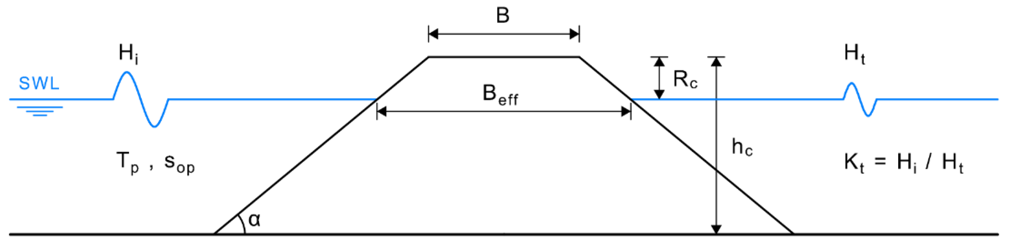
3.2. Wave Transmission at Coastal Structures

Following the rationale presented in Section 1, coastal structures design is treated in this work as a means to countermeasure storm-induced flooding in present and future climates. With the focus set on the transmissivity of low-crested structures, the capability of the presented advanced nearshore wave propagation model in the representation of wave energy reduction behind LCS is validated through comparison with the formulation presented by Goda and Ahrens [34] for Kt. Furthermore, and considering that due to the interplay between wave overtopping and wave infiltration energy reduction is expected to be lower behind impermeable structures than behind permeable ones, the former type of LCS is examined in this work so as to test the lower bound of their effectiveness.
The work of Goda and Ahrens [34] was based on the concept of the summation of wave energy transmitted over and through LCS. The processes were treated separately and two separate transmission coefficients were proposed, namely Kt,over and Kt,thru, respectively, with the summation concept applied for the derivation of Kt using the approach of [66]. The formulation was validated using a versatile set of experimental datasets (851 tests in total), yielding a determination coefficient of r2 = 0.865.
According to [34] Kt for impermeable structures reduces to Kt,over, which was estimated through empirical fitting to the design diagram of [35] and can be expressed as:
K t , o v e r = max { 0 , ( 1 exp [ a ( R c H i 1 ) ] ) }
where Rc is the crest freeboard and a is expressed as:
a = 0.248 exp [ 0.384 ln ( B e f f L 0 ) ]
In Equation (22) L0 is the deep water wavelength and Beff is the effective width of the structure, measured at still water level for emerged structures, at the level of 10% below the crest for zero freeboard structures and at the level of 20% below the crest for submerged structures [34].
Figure 3 shows a sketch of the governing parameters involved in wave transmission at emerged LCS. These are: the incident and transmitted significant wave height, Hi and Ht; the peak period Tp; the wave steepness sop =Hi/g(Tp)2; the crest freeboard and width, Rc and B; the structure height and seaward slope, hc and tanα; and the breaker parameter ξop = tanα/(sop)0.5. Model runs were performed for the series of input parameters presented in Table 1 testing combinations of two incident waves and four different crest freeboards, which resulted in relative freeboards Rc/Hi ranging from 0.13 to 1.00 and relative effective structure widths Beff/L0 ranging from 0.075 to 0.150 (tanα = 0.4 for all runs). The discretization steps used in model (WAVE_BQ) runs were dx = 0.125 m in space and dt = 0.005 s in time. Figure 4 shows the comparison between Kt values as estimated using Equation (21) and as resulted from model runs, for the Tests of Table 1. Data are in good agreement overall, with Test 4 representing a liming case that results in Kt = 0. The model generally predicts lower transmission coefficients than Equation (21). The divergences are mainly observed for higher waves and lower relative freeboard values, a result that is expected considering the concept behind the formulation of [34] and the physics behind the phenomenon.

4. Model Applications

4.1. Large-Scale Applications

The modelling approach for the simulation of flooding over large/regional coastal areas, as presented in Section 2, was applied to the area of the Bay of Thessaloniki, i.e., the northern part of the Thermaikos Gulf, located in the northwestern Aegean Sea, Greece. Thessaloniki is the second largest city in Greece, with a population of approx. 1 million people residing in its metropolitan area. The Port of Thessaloniki is also the second largest in the country, handling a total throughput of approx. 13 million tonnes per year and more than 400,000 containers/TEUs (2018 data; [67]). Two terminals are located west of the Port’s 6th pier, both of significant regional importance. The AGET terminal, whose cement and cement products production and handling facilities include a jetty that extends approximately 600 m into the sea; and the Liquid Fuels Terminal, whose facilities include and offshore jetty located at approximately 800 m from the coast. Figure 5 shows the geographic location and a satellite image of the study area; the six piers of the Port of Thessaloniki are identified, along with the location of the aforementioned facilities.
The model domain was bounded to the south by the virtual East–West line connecting the Mikro Emvolo Cape to the western coast of the Bay (see Figure 6). The intermittently dry/wet area at the western part of the Bay (green dotted area in Figure 6) was modelled as a dry flat for the scenarios run in this work; this is justified by the consideration that the specific area—even when wet at highest tide—is covered by no more than a few centimetres of water (it is noted that small topographic variations over the flat do exist). The domain also included the projected final geometry of the 6th pier of the Port of Thessaloniki (grey crossed area in Figure 6), while it should also be noted that the artificial coast of the Bay of Thessaloniki (Port of Thessaloniki and waterfront eastwards of the Port up to the Mikro Emvolo Cape) was modelled as a solid boundary (i.e., no flooding allowed). This choice served the applications’ computational efficiency, as the waves and storm surges expected in the study area (see Table 2 in the following) are covered by the design of the Port’s piers and the waterfront’s seawalls. The bathymetric data were extracted from digitized nautical charts acquired from the Hellenic Navy Hydrographic Service, while the topographic information was extracted by Digital Elevation Models of the NASA Shuttle Radar Topography Mission, acquired through AppEEARS [69,70].
The models were run for two scenarios of climate change-induced wave and storm surge events, representative for the study area, based on the results and analysis presented by [71]. The first scenario (henceforth denoted by LS1) envisaged a southern wave of significant wave height Hs = 1.58 m and peak period Tp = 4.60 s. The second scenario (LS2) envisaged the same wave combined with a storm surge of height SSH = 0.30 m (see Table 2). The discretization steps used in model runs were dx = 10.0 m in space and dt = 0.05 s in time for WAVE_LS, and dx = 10.0 m in space and dt = 0.125 s in time for SICIR. It should be noted that dx in large-scale wave propagation models is generally of the order of a wavelength L or less [39,40]. However, the choice of dx also depends on bathymetry and model domain characteristics; rapid bathymetric changes or diffraction effects would require smaller values, such as dx = L/5 [40]. In a modular modelling approach, the spatial step of the circulation model would have to be the same as previously selected due to model interoperability. Finally, the temporal step dt is controlled by the Courant number criterion Cr < 1 (Cr = cdt/dx, where c = (gh)1/2). In this work, the choices for the spatial and temporal discretization of WAVE_LS and SICIR followed the above rules.

4.2. Applications for Coastal Structures Design Evaluation

The modelling approach for the investigation of the effect of coastal structures on flooding, as presented in Section 2, was applied to a typical sandy beach located in the East Macedonia and Thrace Region (northern Greece; see Figure 7). The low-lying coastal areas in the region are not densely populated (the coastal cities Kavala and Alexandroupoli do not compare to the size of Thessaloniki), but do host numerous touristic activities and sites of significant ecological importance (Nestos Delta, Lakes Vistonida and Ismarida wetlands). Furthermore, they are exposed to larger waves in both present and future climates, making them more susceptible to coastal flooding.
Table 3 presents the layouts of the selected beach tested using the advanced nearshore wave propagation model (layouts and profile are presented in Section 5.2). The layouts include one of the unprotected beach, one of the beach protected by a breakwater, and one of the beach protected by a sea dike (henceforth denoted by L1, L2 and L3, respectively). The models were run for two scenarios of climate change- induced wave and storm surge events, representative for the study area, based on the results and analysis presented by [71]. The first scenario (henceforth denoted by CS1) envisaged a southern wave of significant wave height Hs = 5.0 m and peak period Tp = 8.0 s. The second scenario (CS2) envisaged the same wave combined with a storm surge of height SSH = 0.30 m (see Table 4). The discretization steps used in model runs were dx = 0.125 m in space and dt = 0.005 s in time for WAVE_BQ (see Section 4.1 for WAVE_LS and SICIR).

5. Results and Discussion

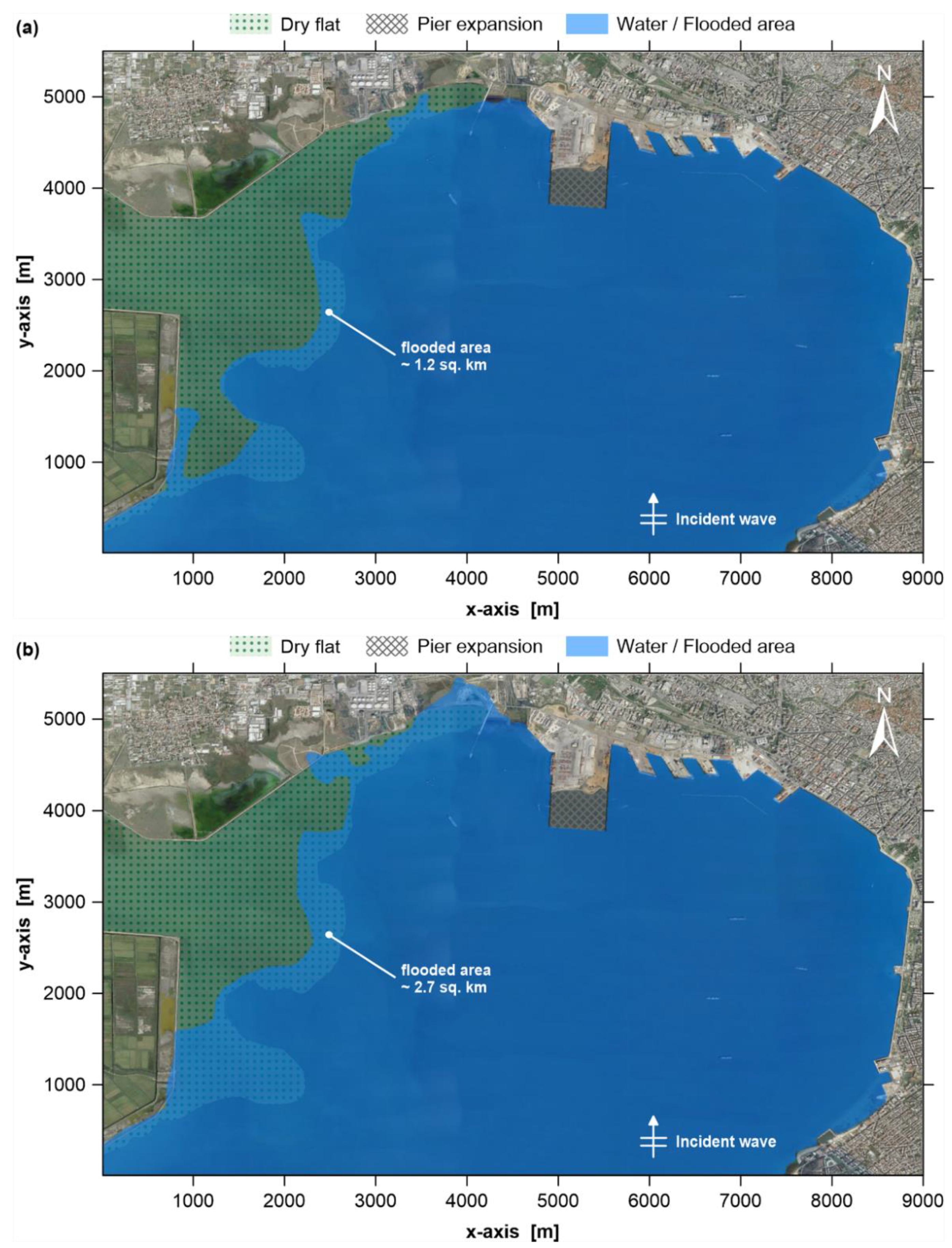
5.1. Large-Scale Applications

Figure 8a shows model results for scenario LS1, indicating the flooded area at the western coast of the Bay of Thessaloniki; Figure 8b shows the respective results for LS2. The models performed satisfactorily in both cases, resulting in smooth flooding contours that follow the modelled topography (it can be noted again that small topographic variations over the flat existed). For scenario LS1 the flooded area mainly covers parts of the aforementioned dry flat, with the flooded area approximately equal to 1.2 km2. For scenario LS2 the flooding extends to the low-lying coastal areas west of the port’s 6th pier as well, with the flooded area approximately equal to 2.7 km2 (increase of approximately 125%). The AGET Terminal appears to be mostly impacted in the case of LS2, while impacts on the operations of both the AGET and liquid fuels jetties are to be expected in either scenario.
Results are indicative of the models capabilities and the potential effects coastal flooding would have on the low-lying areas and operational facilities of coastal cities. Considering that Thessaloniki is located in a relatively protected bay where waves and storm surges are expected to be moderate (as reflected in the selected scenarios in Table 1), it is reasonable to expect more severe flooding in cities exposed to higher storm events, where the overtopping of coastal defence will result in flooding of the urban fabric as well.

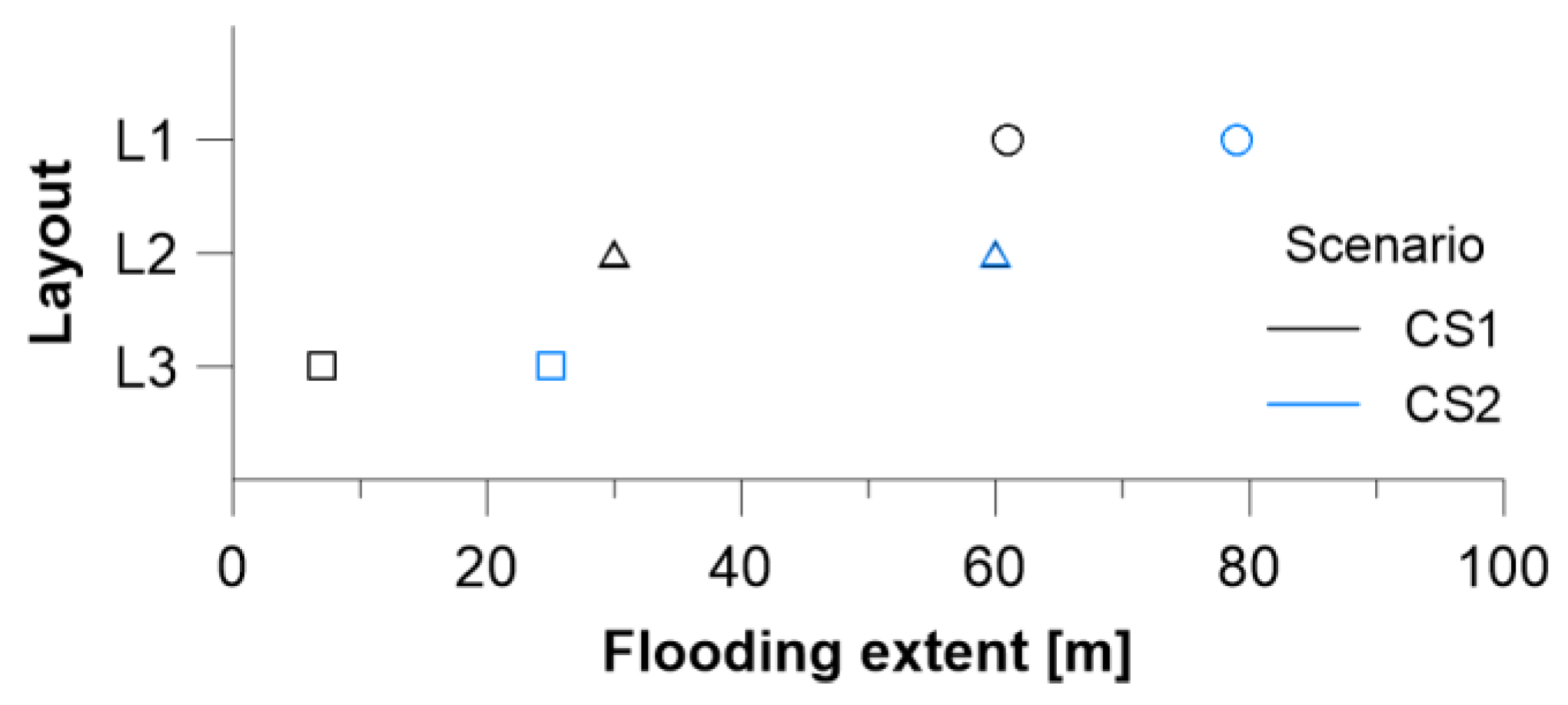
5.2. Applications for Coastal Structures Design Evaluation

Figure 9 shows model results for the six combinations of layouts and scenarios presented in Section 4.2 (see Table 3 and Table 4), as snapshots of surface profile evolution at times T and T + T/2. In Figure 9, coloured “x” symbols denote the landward limit of the flooding extent; this information, expressed as horizontal distance, is comparatively presented for all tests in Figure 10.
As expected, the unprotected beach layout (L1) results in the highest flooding, with storm surge causing an increase in flooding extent by approximately 30% (+18 m). The LCS layout (L2) protects the beach quite satisfactorily for SC1 despite the quite low relative freeboard of the structure (see Table 3 and Table 4), reducing the flooding extent by approximately 51% with respect to L1 (−31 m). However, the addition of storm surge in SC2 practically reduces the emerged crest height and thus cancels a large part of the protection provided by the LCS, resulting in a flooding extent that is increased by approximately 50% (+30 m). It is worth noting that flooding for L2-CS2 is quite close to that of the unprotected beach with no storm surge (L1-CS1), a useful insight for the design of LCS in a changing climate. Finally, the Dike layout (L3) results in the lowest flooding extent, not exceeding 7 m for CS1 (i.e., a reduction of approximately 89% with respect to L1 and of approximately 77% with respect to L2). For SC2, however, the flooding extent more than triples as the wave runs up the slope, reaches the crest of the dike, and propagates inland over the flat. It can be noted that the flat is covered by no more than a few centimetres of water in this test and the flooding extent is still smaller even from L2-SC1; nevertheless, this result is indicative of the function of such structures when facing combinations of increased waves and water levels.

5.3. General Discussion

Elaborating further on the presented modelling system’s performance in simulating coastal flooding, particular insights can be drawn from the following.
Model setup was based on the successful model validation for the representation of coastal flooding and wave transmission at coastal structures, as presented in Section 3.1 and Section 3.2. The satisfactory agreement between model predictions, experimental data and a well-known formulation supported the implementation of the proposed modelling approach to the set of applications presented in Section 4.1 and Section 4.2. These were designed in order to fit two separate modelling objectives, testing all three models of the modelling toolbox and exploring all aspects that are deemed to distinguish this work in relevant literature: (a) the incorporation of an advanced nearshore wave propagation model in the modelling sequence; (b) the accurate representation of the inundation process through the “dry bed” boundary condition; and (c) the capability to test the effect of coastal protection on coastal flooding by simulating wave overtopping and transmission at coastal structures.
The results presented in Section 5.1 and Section 5.2 are indicative of the models’ capabilities, while highlighting the need and importance of relevant works for coastal cities with exposed coastal facilities, as well as for other low-lying coastal areas of ecological, cultural or touristic importance. Future work can explore the limitations of the modelling approach presented by investigating three-dimensional wave–structure interactions and their impact on the identification of flooded areas; work on the same path can also extend to investigate coastal flooding of the urban fabric and combine flooding extent results with damage cost models (e.g., [72,73]).

6. Conclusions

Coastal flooding is on the rise in many areas around the world. The risk of coastal flooding is expected to further increase in the future, as tides, surges and waves will be significantly affected by climate change and the consequent increase of extreme weather events. Numerical modelling can be used to capture the interplay between waves and water levels acting over a broad range of scales in space and time, with relevant modelling systems producing results of direct use for effective design of coastal protection and adaptation measures.
This work presents an in-house, versatile tool for the representation of coastal flooding, which follows a modular modelling approach and consists of three models: a large-scale wave propagation model, a storm-induced circulation model and an advanced nearshore wave propagation model based on the higher order Boussinesq-type equations for breaking and non-breaking waves. The numerical model at the higher-resolution end of the modelling sequence is validated through comparison with the experimental data by Roeber et al. [38] (coastal flooding) and with the formulation of Goda and Ahrens [34] (wave transmission at coastal structures), performing very well for all tests. The proposed modelling approach was applied to simulate coastal flooding: (a) over the low-lying areas of the Bay of Thessaloniki, a semi-enclosed bay located in northern Greece that hosts a major coastal city and significant economic activities; and (b) on a typical sandy beach of the East Macedonia and Thrace Region (also in northern Greece), testing two layouts of coastal protection structures in order to evaluate their effectiveness. Applications for both cases were made for projected scenarios of climate change-induced wave and storm surge events, representative of the respective study areas. Results highlighted the potential effects coastal flooding would have on the low-lying areas and operational facilities of coastal cities, as well as the function of typical coastal protection structures in the above context.
This paper is among the few in relevant literature that incorporate an advanced wave model to a modelling system aimed at representing coastal flooding, along with the accurate representation of the inundation process through a straightforward boundary condition and the capability to test different layouts in order to assess the effect of coastal protection. Drawing insights from the full body of work presented here and relevant literature, this study is considered as a solid example of how the use of advanced modelling tools can facilitate strategic planning and adaptation in coastal areas, shaping the pathways towards a successful response to climate change.

Author Contributions

Conceptualization, methodology, model development, model validation, model applications, formal analysis, visualization, writing, A.G.S. and T.V.K. Both authors have read and agreed to the published version of the manuscript.

Funding

This research received no external funding.

Institutional Review Board Statement

Not applicable.

Informed Consent Statement

Not applicable.

Data Availability Statement

Data is contained within the article.

Conflicts of Interest

The authors declare no conflict of interest.

References

  1. Mentaschi, L.; Vousdoukas, M.I.; Voukouvalas, E.; Dosio, A.; Feyen, L. Global changes of extreme coastal wave energy fluxes triggered by intensified teleconnection patterns. Geophys. Res. Lett. 2017, 44, 2416–2426. [Google Scholar] [CrossRef]
  2. Vousdoukas, M.I.; Mentaschi, L.; Voukouvalas, E.; Verlaan, M.; Feyen, L. Extreme sea levels on the rise along Europe’s coasts. Earth’s Future 2017, 5, 304–323. [Google Scholar] [CrossRef]
  3. Lobeto, H.; Menendez, M.; Losada, I.J. Future behavior of wind wave extremes due to climate change. Sci. Rep. 2021, 11, 7869. [Google Scholar] [CrossRef] [PubMed]
  4. Coelho, C.; Silva, R.; Veloso-Gomes, F.; Taveira-Pinto, F. Potential effects of climate change on northwest Portuguese coastal zones. ICES J. Mar. Sci. 2009, 66, 1497–1507. [Google Scholar] [CrossRef] [Green Version]
  5. O’Grady, J.G.; Hemer, M.A.; McInnes, K.L.; Trenham, C.E.; Stephenson, A.G. Projected incremental changes to extreme wind-driven wave heights for the twenty-first century. Sci. Rep. 2021, 11, 8826. [Google Scholar] [CrossRef] [PubMed]
  6. Kirezci, E.; Young, I.R.; Ranasinghe, R.; Muis, S.; Nicholls, R.J.; Lincke, D.; Hinkel, J. Projections of global-scale extreme sea levels and resulting episodic coastal flooding over the 21st Century. Sci. Rep. 2020, 10, 11629. [Google Scholar] [CrossRef] [PubMed]
  7. Bosello, F.; Nicholls, R.J.; Richards, J.; Roson, R.; Tol, R.S.J. Economic impacts of climate change in Europe: Sea-level rise. Clim. Chang. 2012, 112, 63–81. [Google Scholar] [CrossRef] [Green Version]
  8. Hanson, S.; Nicholls, R.; Ranger, N.; Hallegatte, S.; Corfee-Morlot, J.; Herweijer, C.; Chateau, J. A global ranking of port cities with high exposure to climate extremes. Clim. Chang. 2011, 104, 89–111. [Google Scholar] [CrossRef] [Green Version]
  9. Hinkel, J.; Lincke, D.; Vafeidis, A.T.; Perrette, M.; Nicholls, R.J.; Tol, R.S.J.; Marzeion, B.; Fettweis, X.; Ionescu, C.; Levermann, A. Coastal flood damage and adaptation costs under 21st century sea-level rise. Proc. Natl. Acad. Sci. USA 2014, 111, 3292–3297. [Google Scholar] [CrossRef] [Green Version]
  10. Izaguirre, C.; Losada, I.J.; Camus, P.; Vigh, J.L.; Stenek, V. Climate change risk to global port operations. Nat. Clim. Chang. 2021, 11, 14–20. [Google Scholar] [CrossRef]
  11. Vousdoukas, M.I.; Mentaschi, L.; Voukouvalas, E.; Bianchi, A.; Dottori, F.; Feyen, L. Climatic and socioeconomic controls of future coastal flood risk in Europe. Nat. Clim. Chang. 2018, 8, 776–780. [Google Scholar] [CrossRef]
  12. Rodriguez-Delgado, C.; Bergillos, R.J.; Iglesias, G. Coastal infrastructure operativity against flooding—A methodology. Sci. Total Environ. 2020, 719, 137452. [Google Scholar] [CrossRef] [PubMed]
  13. Wong, P.P.; Losada, I.J.; Gattuso, J.-P.; Hinkel, J.; Khattabi, A.; McInnes, K.L.; Saito, Y.; Sallenger, A. Coastal systems and low-lying areas. In Climate Change 2014: Impacts, Adaptation, and Vulnerability. Part A: Global and Sectoral Aspects. Contribution of Working Group II to the Fifth Assessment Report of the Intergovernmental Panel on Climate Change; Field, C.B., Barros, V.R., Dokken, D.J., Mach, K.J., Mastrandrea, M.D., Bilir, T.E., Chatterjee, M., Ebi, K.L., Estrada, Y.O., Genova, R.C., et al., Eds.; Cambridge University Press: Cambridge, UK; New York, NY, USA, 2014; pp. 361–409. [Google Scholar]
  14. Hubbert, G.D.; McInnes, K.L. A storm surge inundation model for coastal planning and impact studies. J. Coast. Res. 1999, 15, 168–185. [Google Scholar]
  15. Zokagoa, J.M.; Soulaïmani, A. Modeling of wetting-drying transitions in free surface flows over complex topographies. Comput. Methods Appl. Mech. Eng. 2010, 199, 2281–2304. [Google Scholar] [CrossRef]
  16. Barnard, P.L.; Erikson, L.H.; Foxgrover, A.C.; Hart, J.A.F.; Limber, P.; O’Neill, A.C.; van Ormondt, M.; Vitousek, S.; Wood, N.; Hayden, M.K.; et al. Dynamic flood modeling essential to assess the coastal impacts of climate change. Sci. Rep. 2019, 9, 4309. [Google Scholar] [CrossRef] [Green Version]
  17. Bates, P.D.; Dawson, R.J.; Hall, J.W.; Horritt, M.S.; Nicholls, R.J.; Wicks, J.; Ali Mohamed Hassan, M.A. Simplified two-dimensional numerical modelling of coastal flooding and example applications. Coast. Eng. 2005, 52, 793–810. [Google Scholar] [CrossRef]
  18. Gaeta, M.G.; Bonaldo, D.; Samaras, A.G.; Carniel, S.; Archetti, R. Coupled Wave-2D Hydrodynamics Modeling at the Reno River Mouth (Italy) under Climate Change Scenarios. Water 2018, 10, 1380. [Google Scholar] [CrossRef] [Green Version]
  19. Le Roy, S.; Pedreros, R.; André, C.; Paris, F.; Lecacheux, S.; Marche, F.; Vinchon, C. Coastal flooding of urban areas by overtopping: Dynamic modelling application to the Johanna storm (2008) in Gâvres (France). Nat. Hazards Earth Syst. Sci. 2015, 15, 2497–2510. [Google Scholar] [CrossRef] [Green Version]
  20. Li, N.; Roeber, V.; Yamazaki, Y.; Heitmann, T.W.; Bai, Y.; Cheung, K.F. Integration of coastal inundation modeling from storm tides to individual waves. Ocean Model. 2014, 83, 26–42. [Google Scholar] [CrossRef]
  21. McInnes, K.L.; Hubbert, G.D.; Abbs, D.J.; Oliver, S.E. A numerical modelling study of coastal flooding. Meteorol. Atmos. Phys. 2002, 80, 217–233. [Google Scholar] [CrossRef]
  22. Peng, M.; Xie, L.; Pietrafesa, L.J. A numerical study of storm surge and inundation in the Croatan-Albemarle- Pamlico Estuary System. Estuar. Coast. Shelf Sci. 2004, 59, 121–137. [Google Scholar] [CrossRef]
  23. Postacchini, M.; Lalli, F.; Memmola, F.; Bruschi, A.; Bellafiore, D.; Lisi, I.; Zitti, G.; Brocchini, M. A model chain approach for coastal inundation: Application to the bay of Alghero. Estuar. Coast. Shelf Sci. 2019, 219, 56–70. [Google Scholar] [CrossRef]
  24. Goda, Y.; Ippen, A.T. Theoretical and Experimental Investigation of Wave Energy Dissipators Composed of Wire Mesh Screens; Massachusetts Institute of Technology, Cambridge Hydrodynamics Lab: Cambridge, MA, USA, 1963; p. 66. [Google Scholar]
  25. Galani, K.A.; Dimou, I.D.; Dimas, A.A. Wave height and setup in the sheltered area of a segmented, detached, rubble-mound, zero-freeboard breakwater on a steep beach. Ocean Eng. 2019, 186, 106124. [Google Scholar] [CrossRef]
  26. Koutrouveli, T.I.; Dimas, A.A. Wave and hydrodynamic processes in the vicinity of a rubble-mound, permeable, zero-freeboard break water. J. Mar. Sci. Eng. 2020, 8, 206. [Google Scholar] [CrossRef] [Green Version]
  27. Papadimitriou, A.G.; Chondros, M.K.; Metallinos, A.S.; Memos, C.D.; Tsoukala, V.K. Simulating wave transmission in the lee of a breakwater in spectral models due to overtopping. Appl. Math. Model. 2020, 88, 743–757. [Google Scholar] [CrossRef]
  28. Zhang, S.X.; Li, X. Design formulas of transmission coefficients for permeable breakwaters. Water Sci. Eng. 2014, 7, 457–467. [Google Scholar]
  29. Formentin, S.M.; Zanuttigh, B.; Van Der Meer, J.W. A neural network tool for predicting wave reflection, overtopping and transmission. Coast. Eng. J. 2017, 59, 1750006-1. [Google Scholar] [CrossRef]
  30. Panizzo, A.; Briganti, R. Analysis of wave transmission behind low-crested breakwaters using neural networks. Coast. Eng. 2007, 54, 643–656. [Google Scholar] [CrossRef]
  31. d’Angremond, K.; Van der Meer, J.W.; de Jong, R.J. Wave transmission at low-crested breakwaters. In 25th International Conference of Coastal Engineering; ASCE: Orlando, FL, USA, 1996; pp. 2418–2426. [Google Scholar]
  32. van der Meer, J.W.; Briganti, R.; Zanuttigh, B.; Wang, B. Wave transmission and reflection at low-crested structures: Design formulae, oblique wave attack and spectral change. Coast. Eng. 2005, 52, 915–929. [Google Scholar] [CrossRef]
  33. Buccino, M.; Calabrese, M. Conceptual approach for prediction of wave transmission at low-crested breakwaters. J. Waterw. Port. Coast. Ocean Eng. 2007, 133, 213–224. [Google Scholar] [CrossRef]
  34. Goda, Y.; Ahrens, J.P. New formulation of wave transmission over and through low-crested structures. In Proceedings of the Coastal Engineering Conference, Hamburg, Germany; 2009; pp. 3530–3541. [Google Scholar]
  35. Tanaka, N. Wave deformation and beach stabilization capacity of wide crested submerged breakwaters. In 23rd Japanese Conference on Coastal Engineering; JSCE: Tokyo, Japan, 1976; pp. 152–157. [Google Scholar]
  36. Numata, A. Experimental study on wave attenuation by block mound breakwaters. In 22nd Japanese Conference on Coastal Engineering; JSCE: Tokyo, Japan, 1975; pp. 501–505. [Google Scholar]
  37. Tomasicchio, G.R.; D’Alessandro, F. Wave energy transmission through and over low crested breakwaters. J. Coast. Res. 2013, 398–403. [Google Scholar] [CrossRef]
  38. Roeber, V.; Cheung, K.F.; Kobayashi, M.H. Shock-capturing Boussinesq-type model for nearshore wave processes. Coast. Eng. 2010, 57, 407–423. [Google Scholar] [CrossRef]
  39. Booij, N.; Ris, R.C.; Holthuijsen, L.H. A third-generation wave model for coastal regions: 1. Model description and validation. J. Geophys. Res. Oceans 1999, 104, 7649–7666. [Google Scholar] [CrossRef] [Green Version]
  40. Holthuijsen, L.H.; Herman, A.; Booij, N. Phase-decoupled refraction–diffraction for spectral wave models. Coast. Eng. 2003, 49, 291–305. [Google Scholar] [CrossRef]
  41. Battjes, J.A.; Stive, M.J.F. Calibration and verification of a dissipation model for random breaking waves. J. Geophys. Res. Oceans 1985, 90, 9159–9167. [Google Scholar] [CrossRef]
  42. Battjes, J.A.; Janssen, J.P.F.M. Energy loss and set-up due to breaking of random waves. In Proceedings of the 16th International Conference on Coastal Engineering, Hamburg, Germany, 27 August–3 September 1978; pp. 569–587. [Google Scholar]
  43. Leont’Yev, I.O. Modelling of morphological changes due to coastal structures. Coast. Eng. 1999, 38, 143–166. [Google Scholar] [CrossRef]
  44. Koutitas, C.G. Mathematical Models in Coastal Engineering; Pentech Press: London, UK, 1988. [Google Scholar]
  45. Kobayashi, N.; Agarwal, A.; Johnson, B.D. Longshore current and sediment transport on beaches. J. Waterw. Port. Coast. Ocean Eng. 2007, 133, 296–304. [Google Scholar] [CrossRef]
  46. Madsen, P.A.; Rugbjerg, M.; Warren, I.R. Subgrid modelling in depth integrated flows. In 21st International Conference on Coastal Engineering; CERC: Terremolinos, Spain, 1988; pp. 505–511. [Google Scholar]
  47. Militello, A.; Reed, C.W.; Zundel, A.K.; Kraus, N.C. Two-Dimensional Depth-Averaged Circulation Model M2D: Version 2.0, Report 1, Technical Documentation and User’s Guide; ERDC/CHL TR-04-2; US Army Corps of Engineers, Engineering Research and Development Center: Washington, DC, USA, 2004; p. 134. [Google Scholar]
  48. Chen, H.; Jiang, D.; Tang, X.; Mao, H. Evolution of irregular wave shape over a fringing reef flat. Ocean Eng. 2019, 192, 106544. [Google Scholar] [CrossRef]
  49. Chen, Q.; Kirby, J.; Dalrymple, R.; Kennedy, A.; Chawla, A. Boussinesq Modeling of Wave Transformation, Breaking, and Runup.II: 2D. J. Waterw. Port Coast. Ocean Eng. 2000, 126, 48–56. [Google Scholar] [CrossRef]
  50. Pinault, J.; Morichon, D.; Roeber, V. Estimation of Irregular Wave Runup on Intermediate and Reflective Beaches Using a Phase-Resolving Numerical Model. J. Mar. Sci. Eng. 2020, 8, 993. [Google Scholar] [CrossRef]
  51. Roeber, V.; Cheung, K.F. Boussinesq-type model for energetic breaking waves in fringing reef environments. Coast. Eng. 2012, 70, 1–20. [Google Scholar] [CrossRef]
  52. Tang, J.; Zhao, C.; Shen, Y. Numerical investigation of the effects of coastal vegetation zone width on wave run-up attenuation. Ocean Eng. 2019, 189, 106395. [Google Scholar] [CrossRef]
  53. Tonelli, M.; Petti, M. Numerical simulation of wave overtopping at coastal dikes and low-crested structures by means of a shock-capturing Boussinesq model. Coast. Eng. 2013, 79, 75–88. [Google Scholar] [CrossRef]
  54. Zhang, T.; Lin, Z.-H.; Huang, G.-Y.; Fan, C.-M.; Li, P.-W. Solving Boussinesq equations with a meshless finite difference method. Ocean Eng. 2020, 198, 106957. [Google Scholar] [CrossRef]
  55. Brocchini, M. A reasoned overview on Boussinesq-type models: The interplay between physics, mathematics and numerics. Proc. R. Soc. A Math. Phys. Eng. Sci. 2013, 469, 20130496. [Google Scholar] [CrossRef] [Green Version]
  56. Karambas, T.V.; Karathanassi, E.K. Longshore sediment transport by nonlinear waves and currents. J. Waterw. Port. Coast. Ocean Eng. 2004, 130, 277–286. [Google Scholar] [CrossRef]
  57. Schäffer, H.A.; Madsen, P.A.; Deigaard, R. A Boussinesq model for waves breaking in shallow water. Coast. Eng. 1993, 20, 185–202. [Google Scholar] [CrossRef]
  58. Chen, Q.; Dalrymple, R.A.; Kirby, J.T.; Kennedy, A.B.; Haller, M.C. Boussinesq modeling of a rip current system. J. Geophys. Res. Oceans 1999, 104, 20617–20637. [Google Scholar] [CrossRef]
  59. Zou, Z.L. Higher order Boussinesq equations. Ocean Eng. 1999, 26, 767–792. [Google Scholar] [CrossRef]
  60. Wei, G.; Kirby, J. Time-Dependent Numerical Code for Extended Boussinesq Equations. J. Waterw. Port. Coast. Ocean Eng. 1995, 121, 251–261. [Google Scholar] [CrossRef]
  61. Memos, C.D.; Karambas, T.V.; Avgeris, I. Irregular wave transformation in the nearshore zone: Experimental investigations and comparison with a higher order Boussinesq model. Ocean Eng. 2005, 32, 1465–1485. [Google Scholar] [CrossRef]
  62. Polnikov, V.G.; Manenti, S. Study of Relative Roles of Nonlinearity and Depth Refraction in Wave Spectrum Evolution in Shallow Water. Eng. Appl. Comput. Fluid Mech. 2009, 3, 42–55. [Google Scholar] [CrossRef] [Green Version]
  63. Kriezi, E.; Karambas, T. Modelling wave deformation due to submerged breakwaters. Proc. Inst. Civil. Eng. Marit. Eng. 2010, 163, 19–29. [Google Scholar] [CrossRef]
  64. Karambas, T.V.; Samaras, A.G. Soft shore protection methods: The use of advanced numerical models in the evaluation of beach nourishment. Ocean Eng. 2014, 92, 129–136. [Google Scholar] [CrossRef]
  65. Samaras, A.G.; Karambas, T.V.; Archetti, R. Simulation of tsunami generation, propagation and coastal inundation in the Eastern Mediterranean. Ocean Sci. 2015, 11, 643–655. [Google Scholar] [CrossRef] [Green Version]
  66. Wamsley, T.V.; Ahrens, J.P. Computation of Wave Transmission Coefficients at Detached Breakwaters for Shoreline Response Modeling. Coast. Struct. 2003, 2004, 593–605. [Google Scholar]
  67. ThPA S.A.—Thessaloniki Port Authority S.A. Statistical Data 2018; Thessaloniki Port Authority S.A.: Thessaloniki, Greece, 2018; p. 10. [Google Scholar]
  68. Google Earth. Image ©2020 TerraMetrics, Data SIO, NOAA, U.S. Navy, NGA, GEBCO. 2020. [Google Scholar]
  69. NASA JPL. NASA Shuttle Radar Topography Mission Global 1 Arc Second NetCDF; NASA EOSDIS Land Processes DAAC. 2013. [Google Scholar]
  70. AppEEARS Team. Application for Extracting and Exploring Analysis Ready Samples (AppEEARS), Ver. 2.61; NASA EOSDIS Land Processes Distributed Active Archive Center (LP DAAC), USGS/Earth Resources Observation and Science (EROS) Center: Sioux Falls, SD, USA, 2021. [Google Scholar]
  71. Makris, C.; Galiatsatou, P.; Tolika, K.; Anagnostopoulou, C.; Kombiadou, K.; Prinos, P.; Velikou, K.; Kapelonis, Z.; Tragou, E.; Androulidakis, Y.; et al. Climate change effects on the marine characteristics of the Aegean and Ionian Seas. Ocean Dyn. 2016, 66, 1603–1635. [Google Scholar] [CrossRef]
  72. Kirkpatrick, J.I.M.; Olbert, A.I. Modelling the effects of climate change on urban coastal-fluvial flooding. J. Water Clim. Chang. 2020, 11, 270–288. [Google Scholar] [CrossRef] [Green Version]
  73. Ujeyl, G.; Rose, J. Estimating Direct and Indirect Damages from Storm Surges: The Case of Hamburg—Wilhelmsburg. Coast. Eng. J. 2015, 57, 1540006-1540001-1540006-1540026. [Google Scholar] [CrossRef]
Figure 1. Surface profiles of solitary wave transformation over a dry reef flat with A/d = 0.5 and a 1:5 slope. Solid lines denote the results of the presented advanced nearshore wave propagation model (see Section 2.3) and circles denote the measurements of [38].
Jmse 09 01008 g001
Figure 2. Surface profiles of solitary wave transformation over an exposed reef crest with A/d = 0.3 and a 1:12 slope. Solid lines denote the results of the presented advanced nearshore wave propagation model (see Section 2.3) and circles denote the measurements of [38].
Jmse 09 01008 g002
Figure 3. Governing parameters involved in wave transmission at emerged low-crested structures (LCS).
Jmse 09 01008 g003
Figure 4. Wave transmission at emerged LCS: comparison between between Kt values as estimated following [34] and as resulted from the presented advanced nearshore wave propagation model runs (see Section 2.3).
Jmse 09 01008 g004
Figure 5. Geographic location and satellite image of the study area ([68]; privately processed).
Jmse 09 01008 g005
Figure 6. Model domain and bathymetry (background image from [68]; privately processed).
Jmse 09 01008 g006
Figure 7. Geographic location and satellite image of the East Macedonia and Thrace Region ([68]; privately processed).
Jmse 09 01008 g007
Figure 8. Model results indicating the flooded area for scenarios: (a) LS1 and (b) LS2 (background image from [68]; privately processed).
Jmse 09 01008 g008
Figure 9. Model results for the combinations of layouts L1, L2, L3 and scenarios CS1 and CS2. Coloured “x” symbols denote the landward limit of the flooding extent.
Jmse 09 01008 g009aJmse 09 01008 g009b
Figure 10. Flooding extent for the combinations of layouts L1, L2, L3 and scenarios CS1 and CS2. Flooding extent is measured from the shoreline at SWL (horizontal distance).
Jmse 09 01008 g010
Table 1. Values of the parameters in the wave transmission Tests (sop = wave steepness; tanα = slope; ξop = breaker parameter; Rc/Hi = relative freeboard; B/Hi = relative crest width; Beff/L0 = relative effective structure width).
TestsoptanαξopRc/HiB/HiBeff/L0
10.020.42.830.252.50.075
20.500.100
30.750.125
41.000.150
50.040.42.000.131.30.075
60.250.100
70.380.125
80.500.150
Table 2. Scenarios used for the large-scale applications.
ScenarioWaveStorm Surge
Hs (m)Tp (s)Dir (deg)SSH (m)
LS11.584.600-
LS21.584.6000.30
Table 3. Layouts used for the applications for coastal structures design evaluation.
LayoutStructure Characteristics
Typetanα (-)Β (m)Rc1 (m)
L1Unprotected beach
L2LCS0.45.01.0
L3Dike0.2-2.0
1 Measured from SWL.
Table 4. Scenarios used for the applications for coastal structures design evaluation.
ScenarioWaveStorm Surge
Hs (m)Tp (s)Dir (deg)SSH (m)
CS15.08.00-
CS25.08.000.30
Publisher’s Note: MDPI stays neutral with regard to jurisdictional claims in published maps and institutional affiliations.

