A Comparative Study of Model Predictive Control and Optimal Causal Control for Heaving Point Absorbers

Abstract

Efforts by various researchers in recent years to design simple causal control laws that can be applied to WEC devices suggest that these controllers can yield similar levels of energy output as those of more complex non-causal controllers. However, most studies were established without adequately considering device and power conversion system constraints which are relevant design drivers from a cost and economic point of view. It is therefore imperative to understand the benefits of MPC compared to causal control from a performance and constraint handling perspective. In this paper, we compare linear MPC to a casual controller that incorporates constraint handling to benchmark its performance on a one DoF heaving point absorber in a range of wave conditions. Our analysis demonstrates that MPC provides significant performance advantages compared to an optimized causal controller, particularly if significant constraints on device motion and/or forces are imposed. We further demonstrate that distinct control performance regions can be established that correlate well with classical point absorber and volumetric limits of the wave energy conversion device.

1. Introduction

As the field of wave energy conversion transitions from traditional passive control techniques to advanced optimal control strategies for power maximization, it becomes increasingly important to understand the requirements, capabilities, limitations, and benefits of each method to choose the best optimization strategy for a given application.

The control system affects power capture, structural loads, and power-takeoff (PTO) design. To achieve true economic optimality in a wave energy conversion system design, the control system needs to be able to optimize performance given the constraints imposed by the wave energy converter (WEC) system. This is due to the fact that economic outcomes are optimized if a given component or sub-system is continually utilized at its rated operational condition during a majority of its operational life. These rated operational conditions provide constraints within which the device needs to operate, and the WEC control system is responsible for enforcing these constraints because exceeding them will result in mechanical breakdown. As such, the constraint handling of a controller is incredibly important to maximize the economic competitiveness of a WEC device. Constrained optimal control as offered by a Model Predictive Control (MPC) algorithm framework, which is also referred to as non-causal control, is a key tool in this optimization process.

Control systems for wave energy conversion are broadly classified as either causal or non-causal controllers. A causal controller uses information from sensors that monitor the outputs of a dynamical system, in our case the WEC. The sensor information is used as feedback by the controller to follow a desired command signal. Non-causal controllers such as MPC leverage wave prediction to generate control commands in a feed-forward manner rather than using feedback from sensors that measure system output variables. Combination of non-causal (feed-forward) and causal (feedback) control is also possible in a hybrid manner and can be used to correct for modeling and/or wave prediction errors in non-causal controllers.

Within the literature there are two well-published methods for implementing causal control that incorporate constraint handling. The first approach tries to approximate complex conjugate control (CCC) ([1,2,3,4]) with a causal feedback law [5]. This approach does well in the unconstrained case where no motion limits are imposed. To allow for constraints, these methods were subsequently augmented to incorporate an MPC controller that works for the sole purpose of enforcing constraints [5]. Performance of the CCC approximating causal control methods is sub-optimal when constraints are imposed, because the impedance matching value obtained from the CCC approximation provides in-sufficient damping for the constrained case.

The second approach for designing a causal controller comes from recognizing that the causal WEC control problems fall into the Linear Quadratic Gaussian (LQG) paradigm ([6,7,8]). A non-standard LQG optimization problem is established with the objective of maximizing power. The problem treats the input wave excitation force as a stationary stochastic disturbance with a known spectrum. A wave-shaping filter is designed to model the spectrum and this filter model is incorporated in the optimization along with the system dynamics model of the WEC. The LQG optimal controller derived in this manner does not rely on approximations to CCC and will therefore achieve optimality in a broader set of sea states. Stroke protection techniques can be explicitly designed to protect against end-stop violations [7,9]. The control parameters are optimized offline and implemented using a gain schedule to adapt to changing wave conditions. A block-diagram of a casual controller with non-linear stroke protection is shown in Figure 1.

Non-causal performance optimization of WECs is typically implemented using a receding horizon MPC framework. To guarantee optimality, MPC needs a forecast of oncoming waves 20 to 30 s into the future to plan optimal control commands. Wave forecasting can be conducted by placing probes up-wave, measuring the free-surface elevation in the wave field [10], or using a wave-sensing radar [11,12] to characterize the wave-field propagation. These up-wave measurements are marched forward in space and time to predict the wave elevation at the target WEC location. The predicted wave excitation force input, in addition to the states of a system dynamics model, are used to solve a quadratic optimization problem to find the optimal control trajectory. The states of the device are marched forward in time and the optimization process is repeated at each step with new prediction information. Figure 2 shows the basic MPC control architecture.

Considerable research has been undertaken on expanding the capabilities of MPC to meet the requirements of an entire range of device topologies and PTO configurations ([13,14,15,16,17,18,19]). Some of the common constraints that can be handled effectively within the MPC optimization include: (1) PTO force constraints; (2) WEC position, velocity, and acceleration constraints; (3) discrete (ON/OFF) control of PTO forces; and (4) power-flow constraints. MPC can accommodate non-linear device dynamics, such as viscous drag and non-linear models of powertrain losses, which need to be considered in the optimization problem to guarantee optimality [14].

2. Glossary

Variable	Description	Units
g	Acceleration due to gravity	m/s2
$\rho$	Density of sea water	kg/m3
$m$	Mass of the buoy	kg
$m_{\infty }$	Infinite Added Mass	kg
$z$	Displacement of the buoy in heave	m
$\dot{z}$	Velocity of the buoy in heave	m/s
$\ddot{z}$	Acceleration of the buoy in heave	m/s2
$F_R$	Radiation damping force	N
$F_m$	PTO Force	N
$F_s$	Hydrostatic spring stiffness	N
$F_d$	Drag force related to viscous effects	N
$F_e$	Wave excitation force	N
$k$	Buoyancy stiffness coefficient	N/m
$S$	Water plane area of the buoy	m2
$B_{vis}$	Viscous damping coefficient	Ns/m
$C_d$	Drag coefficient	-
$A_r$	A matrix of state space model of the radiation damping sub-system
$B_r$	B matrix of state space model of the radiation damping sub-system
$C_r$	C matrix of state space model of the radiation damping sub-system
$D_r$	D matrix of state space model of the radiation damping sub-system
$X_r$	State vector comprising of all states used to model the radiation damping sub-system in state space form
${\dot{X}}_r$	Vector comprising of the derivatives of all states used to model the radiation damping sub-system in state space form
$n_r$	Number of states used to model the radiation damping sub-system. This is equal to the length of the state vector $X_r$
$0_r$	Row vector of zeros with length $n_r$
$A$	A matrix of WEC state space model
$B$	B matrix of WEC state space model
$C$	C matrix of WEC state space model
$D$	D matrix of WEC state space model
$T_h$	Prediction horizon	s
H	Wave height of a monochromatic wave	m
T	Wave period of a monochromatic wave	s
$H_s$	Significant wave height of a polychromatic wave	m
$T_p$	Peak period of a polychromatic wave	s
$\lambda$	Wavelength	m
$k_w$	Wavenumber
${\overline{P}}_a$	Average absorbed power	W
$v$	Buoy heave velocity	m/s
$h_r$	Radiation impulse-response function	Ns/m
$h_e$	Excitation impulse-response function	N/m
$t$	Time instant	s
$u\left(t\right)$	Control input at time instant t	N
$f_e\left(t\right)$	Wave excitation force at time instant t	N
$x\left(t\right)$	State vector at time instant t comprising of all states used to model the device dynamics
$\dot{x}\left(t\right)$	Derivative of the state vector at time instant t that is used to model the device dynamics

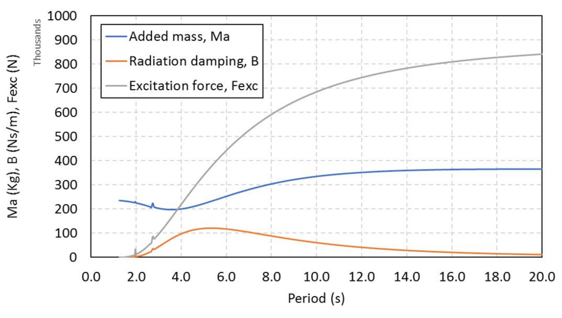
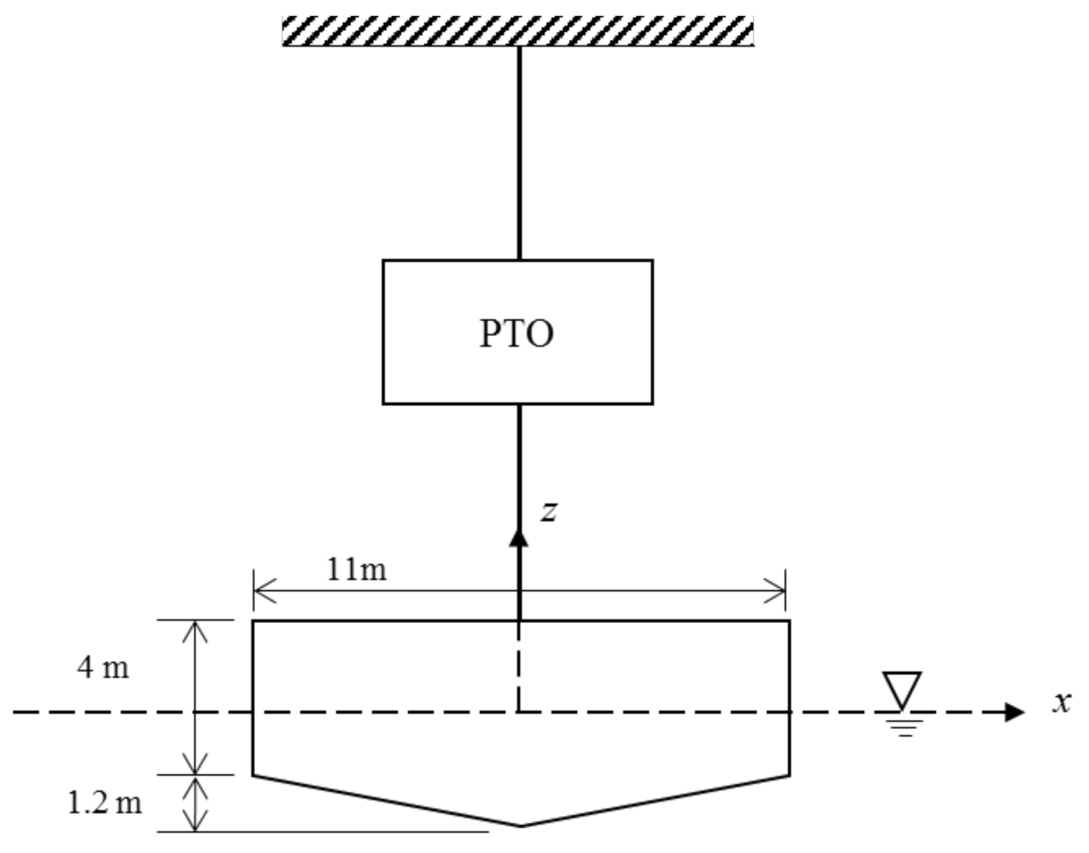
3. The Device Model

We consider a one degree-of-freedom heaving point absorber as an example for our comparison study. A general schematic of the heaving buoy WEC is shown in Figure 3 and key dimensions are provided in

Table 1. Dimensions and physical parameters of the heaving wave energy converter.

Quantity	Value	Units
Buoy diameter	11	m
Buoy cylinder height	4	m
Reaction diameter	11	m
Buoy conical height	1.2	m
Motion limits	±2	m
Buoy mass	228,080	kg
Water Plane Area (S)	95	m2
Coefficient of Drag (Cd)	0.5

. This device has well-established theoretical limits on power absorption which can be used to identify the design trade-off space for controls optimization.

The device geometry was modeled using a commercially available Boundary Element code called WAMIT [20]. The added mass, radiation damping, and excitation force kernels were obtained as a function of frequency by post-processing the WAMIT outputs. Figure 4 shows the frequency dependent parameters plotted against the wave period.

Because this floating body is constrained to move in heave, the equation of motion in the vertical direction is given by:

$$m \ddot{z}\left(t\right)=F_R\left(t\right)+F_{e }\left(t\right)+F_m\left(t\right)+F_s \left(t\right)+F_d\left(t\right)$$

(1)

where $z$ is the displacement, $\dot{z}$ is the velocity, and $\ddot{z}$ is the acceleration of the buoy in heave. m is the displaced mass of the buoy, $F_R$ is the radiation force, $F_e$ is the wave-excitation force, $F_m$ is the PTO force, $F_s$ is the hydrostatic restoring force given by $F_s=-k z$, where $k$ is the buoyancy stiffness, defined as $k=\rho gS$, where $\rho$ is the water density, $g$ the gravitational constant, and $S$ the water-plane area. $F_d$ is the drag force related to viscous effects in real fluid. The viscous damping coefficient was assumed to be linear according to the relationship $F_d=-B_{vis} v$, where $B_{vis}=0.5 C_d\rho S$. $C_d$ is the drag coefficient and ρ is the water density. The radiation force $f_R\left(t\right)$, can be expressed as:

$$F_R\left(t\right)=-m_{\infty }\ddot{z}\left(t\right)-{{\displaystyle \int }}_{-\infty }^t{h}_r\left(t-\tau \right)\dot{z}\left(\tau \right)d\tau$$

(2)

where $m_{\infty }$ is the infinite frequency added mass and $h_r\left(t\right)$ is the impulse response function of the radiation force. The excitation force $F_e\left(t\right)$ is expressed as:

$$F_e\left(t\right)={{\displaystyle \int }}_{-\infty }^{+\infty }{h}_e\left(t-\tau \right)\overline{\eta }\left(\tau \right)d\tau$$

(3)

where $h_e\left(t\right)$ is the excitation force impulse response function and $\overline{\eta }\left(t\right)$ is the wave elevation at the device location. The impulse response function relating the wave elevation to the excitation force affecting the device is non-causal. The main reason is that the chosen input, i.e., the wave elevation at the device location, is not the direct cause of the output, i.e., the interaction force between the wavefield and the device.

To recast the system dynamics into state-space form, the radiation term can be modelled as an embedded sub-system through the following state-space realization:

$${\dot{X}}_r\left(t\right)=A_r{X}_r\left(t\right)+B_r\dot{z}\left(t\right)$$

(4)

$$f_r\left(t\right)=C_r{X}_r\left(t\right)+D_r\dot{z}\left(t\right)$$

(5)

This leads to the following state-space model:

$$\begin{gathered} \dot{x}\left(t\right)=Ax\left(t\right)+Bu\left(t\right)+B{f}_e\left(t\right) \\ y\left(t\right)=Cx\left(t\right)+Du\left(t\right) \end{gathered}$$

(6)

with

$$A=\left[\begin{array}{ccc}{A}_r& 0& B_r\\ 0& 0& 1\\ -\frac{C_r}{m+m_{\infty }}& -\frac{k}{m+m_{\infty }}& -\frac{B_{vis}+D_r}{m+m_{\infty }}\end{array}\right],B=\left[\begin{array}{c}0\\ 0\\ \frac{1}{m+m_{\infty }}\end{array}\right]C=\left[\begin{array}{ccc}{0}_r& 1& 0\\ 0_r& 0& 1\end{array}\right],D=\left[\begin{array}{c}0\\ 0\end{array}\right]$$

(7)

4. Control Methods

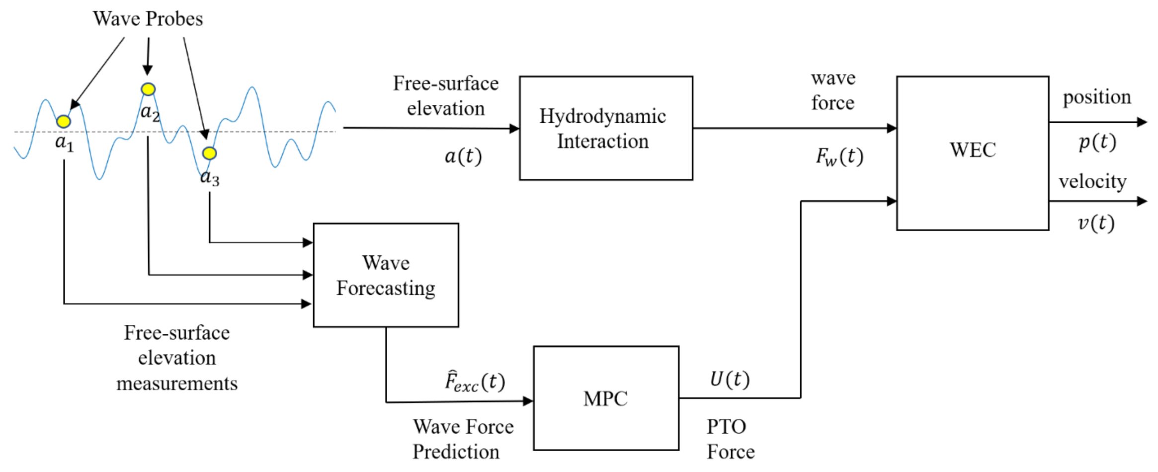
4.1. Model Predictive Control (MPC)

A wave energy converter with a linearized device dynamics model can be optimized using a linear MPC framework. In this type of problem, the non-linearities such as viscous drag are approximated using linear relationships. Under the assumption of no loss in the power generation process, optimizing the device average power absorbed ${\overline{P}}_a$ at a given instant $t_0$ over a defined control horizon $T_h$ can be achieved by determining the optimal control trajectory $u^{*}\left(t\right)$ that maximizes the following cost function:

$${\overline{P}}_a=-\frac{1}{T_h}{{\displaystyle \int }}_{t_0}^{t_0+T_h}v\left(t\right)u\left(t\right)dt$$

(8)

where $v\left(t\right)$ is the instantaneous device velocity. The minus sign is due to the convention of considering absorbed energy with a negative sign. Assuming a fixed time step, we discretize the integral and set up the optimization problem as a minimization by changing the sign in Equation (9). The new optimization objective, therefore, is given by:

$$J=\frac{1}{N}{\displaystyle \sum }_{k=0}^{N-1}{x}_{k+1}^T{S}_v^T{u}_k$$

(9)

where $N$ is the number of time intervals over the control horizon $T_h$ and $S_v$ is a linear operator extracting the WEC velocity from the state-space vector. The control force and state vector, however, are not independent variables, and are constrained by the system dynamics equation of the WEC, which in discrete time is defined as:

$$x_{k+1}=A_d{x}_k+B_d{u}_k+B_d{f}_{e_k},\hspace{1em}k=0, \dots , N-1$$

(10)

with initial condition $x_0={\overline{x}}_0$.

To preserve mechanical and structural integrity, motion constraints and force limits are imposed. These constraints limit the maximum actuation force and the WEC device velocity and vertical displacement, i.e.,

$$u_{min}\le u_k \le u_{max},\hspace{1em}k=0, \dots , N-1$$

(11)

$$p_{min}\le S_p{x}_k \le p_{max},\hspace{1em}k=0, \dots , N$$

(12)

$$v_{min}\le S_v{x}_k \le v_{max},\hspace{1em}k=0, \dots , N$$

(13)

where $S_p$ is a linear operator extracting the WEC displacement from the state vector. The cost function, together with the constraints, represents a linear MPC problem in its standard formulation.

Let us define the following consolidated vectors based on the sequence of states and control commands. This will help in simplifying the notation and problem setup:

$$X={\left[\begin{array}{cccc}{x}_1^T& x_2^T& \dots & x_N^T\end{array}\right]}^T$$

(14)

$$U={\left[\begin{array}{cccc}{u}_1^T& u_2^T& \dots & u_N^T\end{array}\right]}^T$$

(15)

Let us define ${\Lambda }_v$, ${\Lambda }_p$ as block diagonal matrices having the velocity extraction matrix $S_v$ and the position extraction matrix ${\Lambda }_p$, repeated N times respectively on the main block diagonal. Furthermore, let $I$ be the $N\times N$ identity matrix and let $\xi$ be a $N\times 1$ vector of ones. In this manner, the cost function can then be expressed as follows:

$$J=\frac{1}{N} X^T{\Lambda }_v^{T}U$$

(16)

The inequality constraints can be reformulated using this vector notation as follows:

$$D_{u}U\le d_u$$

(17)

$$D_{x}X\le d_x$$

(18)

where

$$D_u=\left[\begin{array}{c}I\\ -I\end{array}\right]d_u=\left[\begin{array}{c}{u}_{max}\ast \xi \\ -u_{min}\ast \xi \end{array}\right]$$

(19)

$$D_x=\left[\begin{array}{c}{\Lambda }_p\\ -{\Lambda }_p\\ \begin{array}{c}{\Lambda }_v\\ -{\Lambda }_v\end{array}\end{array}\right]d_x=\left[\begin{array}{c}{p}_{max}\ast \xi \\ -p_{min}\ast \xi \\ \begin{array}{c}{v}_{max}\ast \xi \\ -v_{min}\ast \xi \end{array}\end{array}\right]$$

(20)

By recursively applying the discrete-time dynamics equations, it is possible to express $X$ as a function of the control vector $U$, the excitation force vector $F_e$, and the initial condition ${\overline{x}}_0$:

$$X={{\rm Y}}_d{\overline{x}}_0+{\Gamma }_{d}U+{\Gamma }_d{F}_e$$

(21)

where

$${{\rm Y}}_d=\left[\begin{array}{c}{A}_d\\ A_d^2\\ ⋮\\ A_d^N\end{array}\right]$$

(22)

$${\Gamma }_d=\left[\begin{array}{cccc}{B}_d& 0& 0& 0\\ A_d{B}_d& B_d& 0& 0\\ ⋮& ⋮& \ddots & 0\\ A_d^{N-1}{B}_d& A_d^{N-2}{B}_d& \dots & B_d\end{array}\right]$$

(23)

$$F_e={\left[\begin{array}{cccc}{f}_{e_0}^T& f_{e_1}^T& \dots & f_{e_{N-1}}^T\end{array}\right]}^T$$

(24)

This allows us to rewrite the MPC problem as the following cost function and constraint equations:

$$\underset{U}{\min }{U}^T{\Gamma }_d^T{\Lambda }_v^{T}U+{\left({\Lambda }_v{{\rm Y}}_d{\overline{x}}_0+{\Lambda }_v{\Gamma }_d{F}_e\right)}^{T}U$$

(25)

$$\left[\begin{array}{c}{D}_u\\ D_x{\Gamma }_d\end{array}\right]U \le \left[\begin{array}{c}{d}_u\\ d_x-D_x{{\rm Y}}_d{\overline{x}}_0-D_x{\Gamma }_d{F}_e\end{array}\right]$$

(26)

The maximization of absorbed power requires the solution of a constrained convex optimization problem, for which well-consolidated routines, such as interior-point-convex or active-set methods, are available in literature [21,22]. Positive definiteness of the Hessian is, in general, guaranteed for the optimization of a point absorber device, unless the time step chosen for the conversion of the continuous time model into discrete time is too large to represent the actual behavior of the WEC device. At each timestep, an MPC problem needs to be solved, and the first value of the optimal solution vector $U^{*}$ is applied to the system. The system is marched forward in time by integrating the system dynamics using a standard Runge–Kutta (RK) scheme. The above MPC formulation also assumes that a perfect excitation force prediction is available 20 to 30 s into the future using up-wave measurement probes.

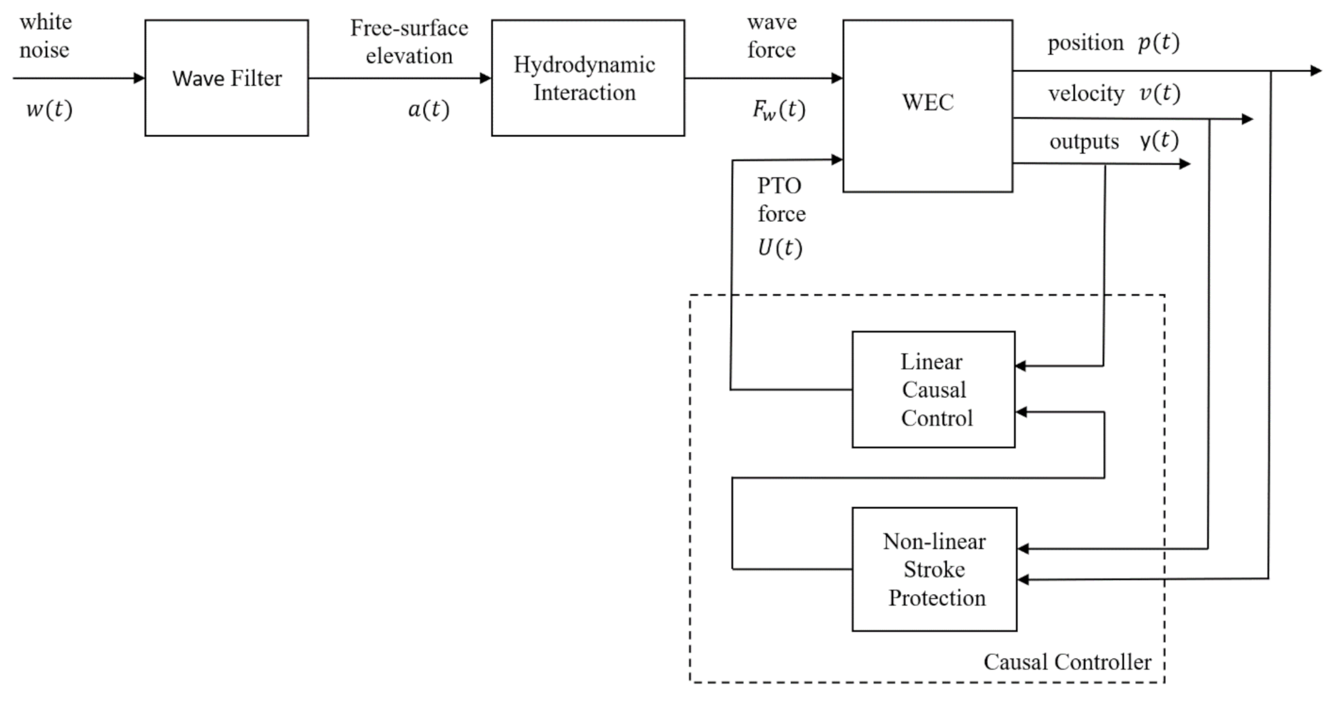
4.2. Causal Feedback Control

The first step in optimal causal feedback control design is to determine an analytically tractable stochastic disturbance model to represent the incident wave force f_e(t). This step is nontrivial for two reasons. Firstly, the power spectral density typically used to characterize the free surface elevation $\overline{\eta }\left(t\right)$, denoted $S_{\eta }\left(\omega \right)$, does not constitute a rational spectrum (i.e., it is not a ratio of rational polynomials of frequency $\omega$). Secondly, the transfer function from the free surface elevation to the incident wave force, equal to

$$H_e\left(s\right)={{\displaystyle \int }}_{-\infty }^{\infty }{e}^{-st}{h}_e\left(t\right)dt$$

involves the solution to a partial differential equation (due to fluid–structure interaction), and consequently it also does not evaluate to a rational transfer function. Consequently, the resultant power spectral density of the incident wave force, denoted as

$$S_e\left(\omega \right)=S_{\eta }\left(\omega \right){\left|H_e\left(j\omega \right)\right|}^2$$

is an irrational function of frequency. To make the causal control design problem tractable, this spectrum must be approximated, as

$$S_e\left(\omega \right)\approx {\left|G\left(j\omega \right)\right|}^2$$

where the transfer function G(s) is a stable, minimum-phase, strictly-proper, rational transfer function. Equivalently, we seek to find matrices A_e, B_e, and C_e such that in the above equation,

$$G\left(s\right)=C_e{\left[sI-A_e\right]}^{-1}{B}_e$$

With such a formulation for G(s), we may equivalently represent the incident wave force as filtered white noise; i.e.,

$${\dot{x}}_e\left(t\right)=A_e{x}_e\left(t\right)+B_{e}w\left(t\right)$$

$$f_e\left(t\right)=C_e{x}_e\left(t\right)$$

where w(t) is a white noise process with unit spectral intensity.

There are a number of ways to find appropriate matrices A_e, B_e, and C_e for the noise filter model described above. Here, we make use of the subspace-based spectral factorization approach. Because this approach is applied exactly as described in [23], we will forgo the details here in the interest of brevity.

With the accomplishment of the finite-dimensional approximation of the incident wave force, we then append the internal states x_e(t) to the state x(t) of the physical system; i.e., we define $x_a\left(t\right)={\left[\begin{array}{cc}{x}^T\left(t\right)& x_e^T\left(t\right)\end{array}\right]}^T$ to arrive at an augmented state space model:

$$\begin{gathered} {\dot{x}}_a\left(t\right)=A_a{x}_a\left(t\right)+B_{a}u\left(t\right)+E_{a}w\left(t\right) \\ y\left(t\right)=C_a{x}_a\left(t\right)+D_{a}u\left(t\right) \end{gathered}$$

where matrices A_a, B_a, E_a, C_a, and D_a are appropriately defined. Our objective is to design a causal feedback law that maps y into u, to maximize the objective

$${\overline{P}}_a=-E\left\{vu+R{u}^2\right\}$$

where E{.} denotes the expectation in stationarity, and R is a nonnegative parameter. For the case in which R = 0, the above expression is simply the mean power absorption. In design, R is typically chosen to be greater than zero, for two reasons. Firstly, it can be used to (approximately) quantify the power dissipation in the power train of the WEC, thus changing the performance objective from absorbed power to generated power. Secondly, it can be used as a tuning parameter to balance the power generation objective against the need to keep the mean-square control force magnitude below a desired threshold.

If there were no constraints on the response of the WEC, the above problem could be solved in closed form. More specifically, it distills to a sign-indefinite Linear Quadratic Gaussian (LQG) control problem, which is guaranteed to have a unique, stabilizing solution assuming that the open-loop mapping from $u$ to $\dot{z}$ is passive [6]. However, for the WEC under consideration here, there are constraints on both the displacement z and the control force u. In the presence of these constraints, the closed-form LQG control solution cannot be used without modification. To address these constraints, in this paper we implement the methodology outlined in detail in [9]. Because the methodology used here is identical to that one, we only provide an overview here of the basic steps in the nonlinear control design procedure.

The first step is to design a linear feedback controller of the form

$$\begin{gathered} \dot{\xi }=A_c\xi +B_{c}y \\ u=C_c\xi \end{gathered}$$

in which A_c, B_c, and C_c are optimized to maximize ${\overline{P}}_a$, subject to two constraints. The first of these constraints is a relaxed version of the WEC displacement constraint, in which we require only that the mean-square displacement be below a bound related to p_max, i.e.,

$$E\left\{z^2\right\}\le \sigma p_{max}^2$$

where $\sigma <1$ is a design parameter, chosen here to be 0.25. The second constraint is the restriction that the open-loop controller must be stable; i.e., that A_c be a Hurwitz matrix. Convex techniques for accomplishing this constrained optimization are covered extensively in [9]. The resultant linear controller is guaranteed to result in positive power generation, be robust to saturations in the input u, and maintain mean-square displacements below $p_{max}^2$. However, it does not guarantee that the displacement limit is satisfied at all times.

The second step is to augment the above linear control design with a nonlinear stroke-protection feedback loop that ensures that the displacement limit is satisfied at all times (rather than just in the mean-square sense). This stroke protection loop, and its relationship to the linear control design, is illustrated in Figure 1. It accepts as inputs the position and velocity, and outputs a supplemental nonlinear force q. This quantity q is sent back to the linear controller through an augmented input matrix, i.e., via the equations:

$$\begin{gathered} \dot{\xi }=A_c\xi +B_{c}y+E_{c}q \\ u=C_c\xi +q \end{gathered}$$

where E_c is a matrix of design parameters. The design of the feedback function that maps $\left\{z,\dot{z}\right\}$ into q, and the design of E_c, are described in fully in [9]. Here it suffices to say that q can be viewed as being similar to the restoring force of a “virtual hardening spring,” providing no force when the displacement is far from its limit, but increasing to infinity when the displacement approaches its limit. The participation of velocity $\dot{z}$ in the function can be thought of as providing damping. Meanwhile, the matrix E_c is designed such that the open-loop transfer function from q to $\dot{z}$ is passive, which guarantees unconditional stability of the closed-loop system.

The controller resulting from the above design framework is guaranteed to protect the displacement from reaching its limit for the case in which the force u is unbounded. When saturation limits are imposed on u, of the form

$$u=\left\{\begin{array}{cc}{u}_{min}:& C_c\xi +q<u_{min}\\ C_c\xi +q:& u_{min}\le C_c\xi +q\le u_{max}\\ u_{max}:& C_c\xi +q>u_{max}\end{array}\right.$$

then the displacement protection is not strictly guaranteed. Indeed, when both the force and displacement are constrained, there may not exist a controller that can honor both. However, proper tuning of the various design parameters in the control design can be undertaken to assure that displacement constraints are satisfied in all but extremely rare cases in stationary response.

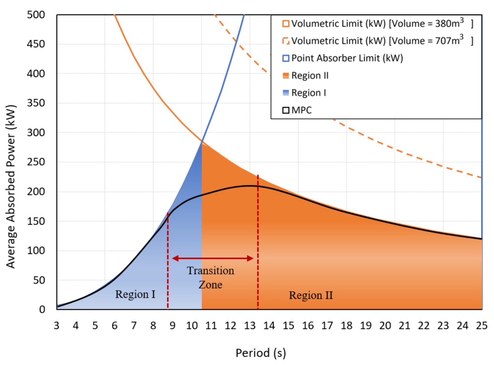
5. Theoretical Limits on the Average Absorbed Power

5.1. Point Absorber Limit

Consider a heaving axisymmetric body oscillating without constraints in resonance with an incoming regular wave of period T (s) and height H (m). Let $J_E$(W/m) denote the wave power level, $k_w$(1/m) denote the wavenumber, and $\lambda$ (m) the wavelength. In this case, the point absorber effect in wave-energy extraction [24] imposes a fundamental limit on the average absorbed power ${\overline{P}}_a$. As described in [24,25], this limit can be derived from the relationship between absorption width $d_a={\overline{P}}_a/J_E\left(m\right)$ and wavelength $\lambda$, as shown below:

$$d_a\le \frac{1}{k_w}=\frac{\lambda }{2\pi }$$

(27)

Or equivalently:

$${\overline{P}}_a\le \frac{1}{k}{J}_E=\frac{\rho }{128}{\left(\frac{g}{\pi }\right)}^3{T}^3{H}^2$$

(28)

The last equality in Equation (28) is valid for deep water conditions. This is referred to as the Point Absorber Limit. The theoretical limit may be reached if the average absorbed power equals half the average excitation power, which happens when the radiated power is equal to the absorbed power. Furthermore, it is known that the Point Absorber Limit can only be reached up to a certain wave period and height. This depends on the motion amplitude constraints on the absorber. Beyond, only a lower relative power absorption can be realized, as defined by a device’s volumetric limit.

5.2. Volumetric Limit

The heaving body sweeps a finite volume during its oscillation cycle based on physical limits. This volumetric constraint imposes a limit on the average power absorbed from each oscillation cycle. As shown in [25], the average power $P_a$ in the motion-constrained case is limited by the expression:

$${\overline{P}}_a<\left(\pi \rho gHV/4T\right)$$

(29)

This is referred to as the volumetric limit. With advanced control, we expect to achieve the active theoretical limit based on the device’s operational region.

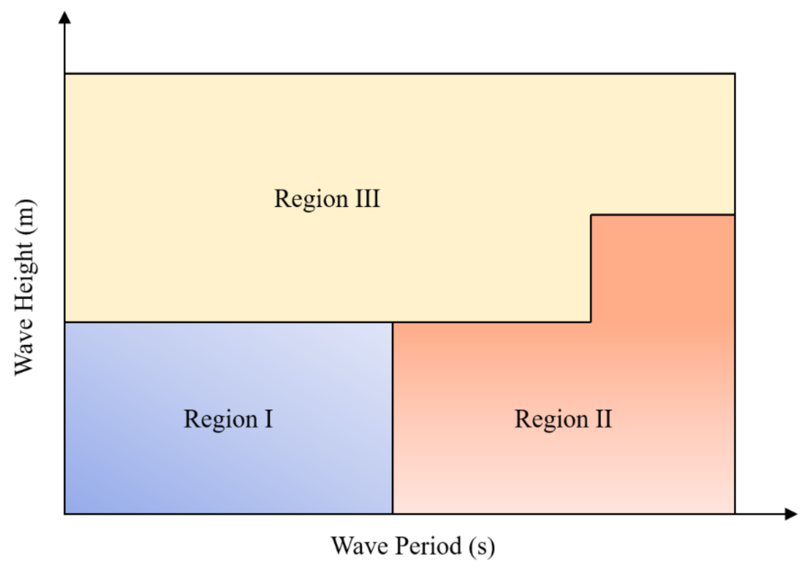
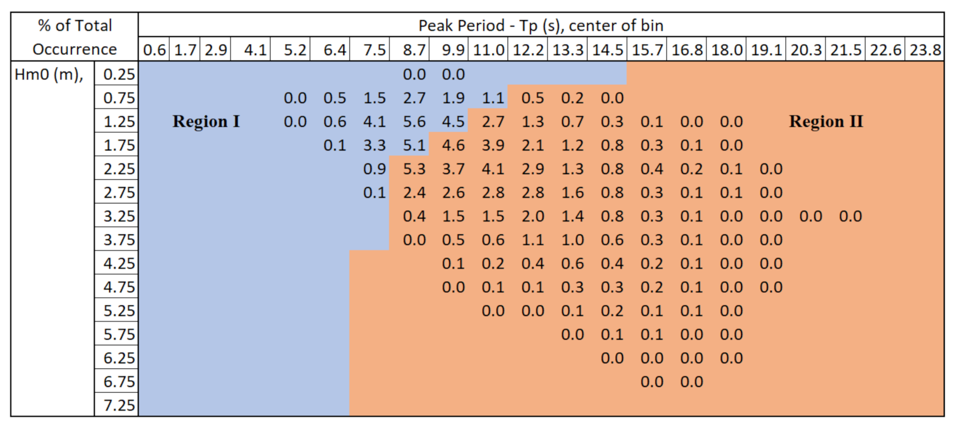
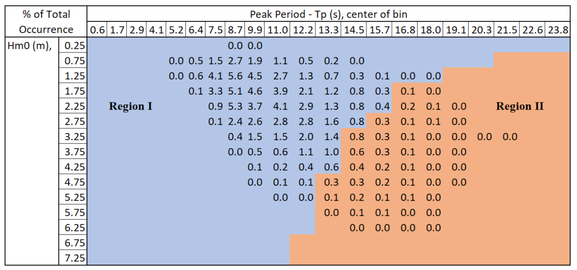
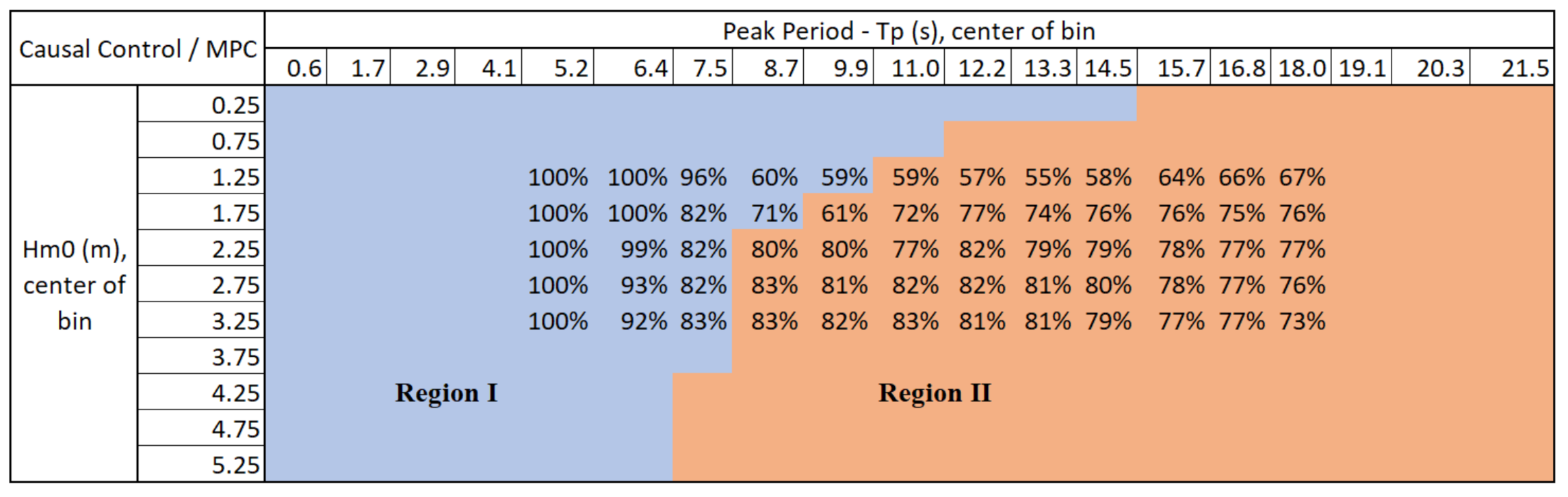
5.3. Controller Design Trade-Off Space

The controller design trade-off space for a WEC is defined by the Point Absorber and Volumetric Limit. For any given wave period, we will call the lesser of the two the “active theoretical limit” or the “theoretical limit” for simplicity. The controller performance cannot exceed the theoretical limit, and this defines the design trade-off space for controller optimization. As shown in Figure 5, the Point Absorber Limit is “active” for shorter wave periods. We will call this set of wave periods Region I. The Volumetric Limit is “active” for longer wave periods and we will call this set of wave periods Region II. The cross-over period, where the Point Absorber and Volumetric Limits are equal, demarcates the two regions.

Equations (28) and (29) show that both upper limits are wave height dependent and describe the WEC device performance in sinusoidal waves. To understand theoretical upper limits for an irregular wave train, we compute the wave height for a sinusoidal wave with the equivalent average power density of the irregular wave train as follows. The power in a monochromatic wave of height H and period T is given by:

$$P_{mono}=H^{2}T$$

(30)

The equivalent wave height (H) of a monochromatic wave with the same power as the polychromatic wave can be found by equating the two. Assuming the period of the monochromatic wave to be the same as the peak period of the polychromatic sea state, we obtain the wave height of the equivalent sinusoidal wave as:

$$H=0.64 H_s$$

(31)

This approach allows us to classify regions in the scatter diagram based on point absorber theory, and to draw meaningful conclusions regarding the importance of MPC-based control. For this purpose, we divided the entire set of input wave conditions into three distinct regions based on theoretical limits. Figure 6 illustrates the partitioning of sea states, where Region $\mathrm{I}$ corresponds to wave conditions where performance is dominated by the Point Absorber Limit. Region $\mathrm{II}$ corresponds to wave conditions where performance is dominated by the Volumetric Limit. Finally, Region $\mathrm{III}$ is associated with large waves where controllers are expected to maintain rated power production and minimize structural loads on the system. Region III is not important from a performance optimization perspective, but it is important that a control law active in this region will continue to produce power at the rated capacity, while minimizing structural loads. Although slightly counter-intuitive, structural loads in Region III can be smaller than those in Regions I and II because we are effectively de-tuning the system to the incident wave conditions.

Applying the above region-based approach to a small and a large heaving point absorber provides the following regions. To understand their significance in context, we simply superimposed the regions onto the frequency distribution of the DoE’s reference resource in Humboldt Bay, California. As shown in Figure 7, the reference geometry used for this paper has only a few sea states, where causal control has the potential to provide similar performance as that of the MPC-based controller. This is in stark contrast to the SANDIA Wavebot, which has a much larger volumetric displacement and as a result performs well in most sea-states using causal control (see Figure 8).

The comparison in

Table 2. Percentage of total sea state occurrence in Regions I and II for the heaving buoy and SANDIA WaveBot.

% of Total Occurrence	Heaving Buoy (Swept Volume = 380 m3)	SANDIA WaveBot (Swept Volume = 4303 m3)
Region I	32%	94%
Region II	68%	6%

shows a buoy with a much larger volumetric displacement, similar to that tested by SANDIA [26]. It shows that fewer regions are present where volumetric limits dominate and, therefore, MPC becomes less important.

6. Results

6.1. Benchmarking Performance of Causal Control Design Methods

To provide a fundamental understanding of the unconstrained controls’ performance, we compared Optimal Causal Control, which is based on the LQG paradigm [7], with SANDIA’s causal controller designed based on the CCC approximation principle–Proportional Integral (PI) and Feedback Resonator (MPC-FBR). A set of MATLAB and Simulink files containing methods for implementing PI and FBR controllers is available online through the Marine Hydro-Kinetic Data Repository [26]. Both controllers were simulated to compare performance in different wave conditions using no wave prediction information. MPC was also simulated with the same inputs to serve as an upper limit for benchmarking performance of the two causal controller design methods.

The results of this initial trade-off study demonstrated that the algorithm provided by SANDIA provided significantly lower power capture across all sea states, but especially in longer-period waves, where the impedance-matching condition of the underlying controls law is physically impossible due to the device’s volumetric constraints. Because we found the LQG method outperformed the CCC controller, the remainder of comparisons in this paper were carried out between the LQG causal control method and a linear MPC controller. Time-domain simulations were carried out using Optimal Causal Control using the LQG method outlined in [9] and linear Model Predictive Control for a complete set of wave conditions. A discrete time-step of 0.01 s and a simulation length of 3600 s was utilized. A Pierson–Moskowitz (PM) wave spectrum with the following formulation was chosen to generate the wave train using the WAFO Toolbox [27]. A plot of the input PM spectrum is shown in Figure 9

$$S\left(\omega \right)=\frac{5H_{m0}^2}{{\omega }_p{\omega }_n^5} e^{-\frac{5}{4} {\omega }_n^{-4}}$$

(32)

where ${\omega }_p=\frac{2\pi }{T_p}$ and ${\omega }_n=\frac{\omega }{{\omega }_p}$.

6.2. Controller Performance with Unconstrained PTO Force

First, let us look at the unconstrained case where no PTO force limits are imposed on the controller. Motion constraints are still enforced because the displacement of the device relative to the equilibrium is limited to ±2 m. Figure 10 shows a plot of the ratio of average absorbed power using causal control normalized to the average absorbed power using MPC. For short period waves, the ratio of causal controller response closely follows that of MPC and the performance ratio is within 90%. This corresponds to Region I, where power absorption is dominated by the Point Absorber Limit. In long-period waves, the performance ratio starts to deteriorate for wave periods >10 s. This corresponds to Region II, where power absorption is dominated by the volumetric constraint. The results show that, unlike in the case of MPC, the stroke-limited power absorption capability of causal controllers is sub-optimal.

Figure 11, Figure 12, Figure 13 and Figure 14 show the time domain comparison of the device response with MPC and causal control for a significant wave height of 1.0 m and Tp = 15 s. The comparison is shown for a wave input in Region II where the volumetric constraint is active. Note that the MPC motion profile often covers the full stroke as opposed to causal control (Figure 13). MPC’s “latching” behavior can also be seen in the velocity response profile.

6.3. Comparison of Annual Average Energy Capture for Reference Site

A simulation study was carried out to benchmark performance of the two control approaches by calculating the overall annual average energy capture for a deep-water reference site. The heaving buoy WEC was simulated for all of the wave conditions in the scatter diagram shown in Figure 7 for the reference site at Humboldt Bay, CA. Both controllers were simulated with a stroke limit of ±2 m, and no limits on the peak PTO force were imposed.

Assuming a plant capacity factor of 30%, we obtained rated power of 473 kW using MPC and 375 kW with causal control (see

Table 3. Performance comparison of MPC and causal control for the DoE reference site at Humboldt Bay, CA, USA.

		MPC	Causal Control
Rated Power (kW)		473	375
Average Power (kW)		142	113
Capacity Factor		30%	30%
% Annual Energy Captured	Region I	19%	18%
	Region II	81%	82%

). At this site, the causal controller captures only 79% of the MPC-based controller.

Figure 10 shows the ratio of average absorbed power between causal control and MPC at each sea state. Note that in the regions which are point absorber limited (Region I), the two controllers perform equally well. For long-period waves where performance is upper bound by the Volumetric Limit (Region II), as expected, MPC outperforms causal control. Overall, we note that the percentage of sea state occurrences in Region II is 67.8% and is responsible for close to 81% of the respective annual energy captured from all sea states.

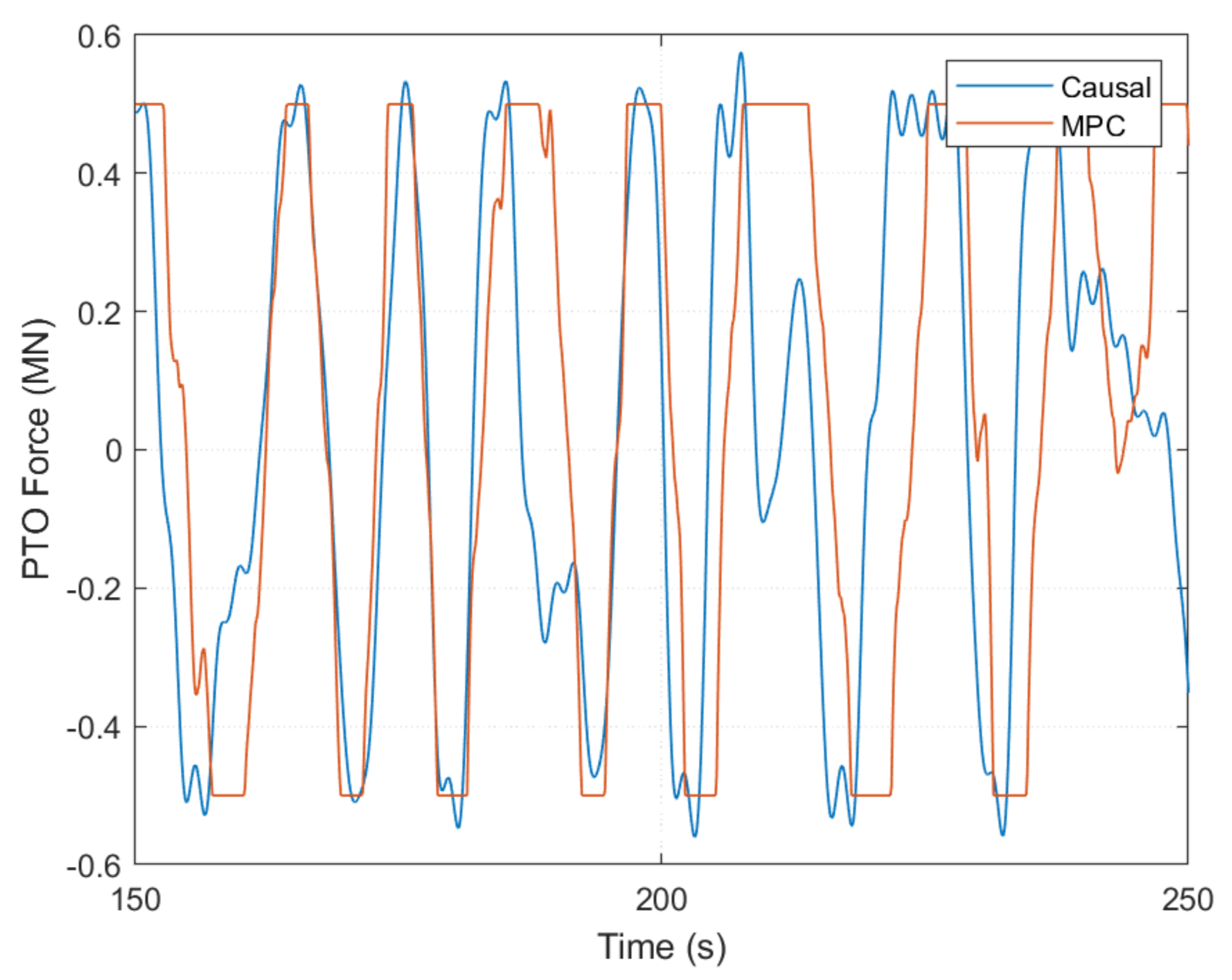
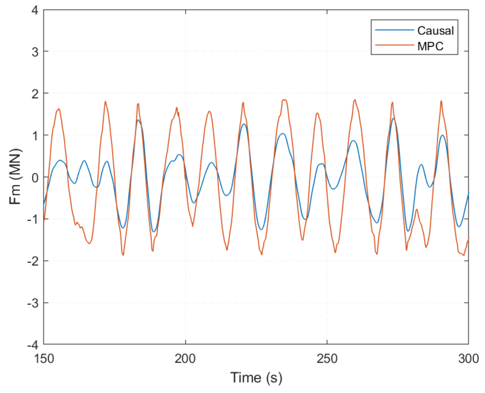
6.4. Controller Performance with Constrained PTO Force

Controllers must often operate with limits imposed on the maximum PTO force due to hardware limitations. Therefore, it is important to determine how well the two control approaches handle force constraints. In this situation, the controller must attempt to maximize power absorption while simultaneously limiting the maximum forces used on the PTO. Not all controllers can achieve this dual objective effectively, which typically results in sub-optimal performance for causal controllers. Figure 15 shows a plot of average power capture vs. force constraint for both control approaches. Note that for the same choice of PTO force limit, the average power capture with MPC significantly exceeds causal control. Another way of interpreting these results is that MPC requires less PTO force to achieve the same power capture performance as that of causal control. Figure 16, Figure 17, Figure 18 and Figure 19 show time domain comparison of the device response with causal control and MPC when the PTO force is limited to 0.5 MN.

In addition to the control commands issued by the linear causal controller, the causal controller also has a non-linear stroke protection block which adds to the requirements of the PTO machinery force. Causal controllers require careful tuning of the non-linear control parameters to reduce spikes in PTO machinery force. Tuning the stroke protection parameters helps to smooth the PTO force response but it comes at the cost of sacrificing the amount of power that is absorbed. Figure 17 shows a comparison of the PTO force response with causal control and MPC. Note that MPC is able to limit the PTO force effectively, and does not violate the force limit. In contrast, causal control occasionally violates the force limit.

7. Conclusions

In this paper, we presented results of a performance comparison study between causal and non-causal methods in a design trade-off space formed by theoretical upper limits on power absorption. While exploring this design trade-off space, we show that identification of operating regions based on device displaced volume and site-specific annual spectrum data are key drivers in identifying suitable control methods for a given WEC application. MPC and causal control performance is similar for Region I, where performance is constrained by Point Absorber Limits and assuming that the PTO is capable of full four-quadrant control. For operating Region II, where performance is limited by Volumetric Limits, MPC shows a significant performance advantage compared to the causal control method.

It should be noted that the cost of most in-ocean systems is directly proportional to their displaced volume. This means that the ratio of average power to volume (P/V) is a key indicator of structural efficiency of a WEC device. Small point absorbers tend to have better P/V ratios, which drives economically viable solutions towards smaller devices. As shown in this study, these smaller point absorbers will produce power predominantly in Region II, where volumetric constraints dominate and MPC provides significant performance advantages. Furthermore, constrained optimal control offered by MPC provides benefits beyond pure performance gains. The ability to directly handle a wide range of constraints as part of the optimization problem ensures constraints can be gently applied, thus reducing transient loads that are harmful to the PTO and device structural components, while maximizing power production.

References

1. Nebel, P. Maximizing the Efficiency of Wave-Energy Plant Using Complex-Conjugate Control. J. Syst. Control Eng. 1992, 206, 225–236. [Google Scholar] [CrossRef]
2. Budal, K.; Falnes, J. Interacting Point Absorbers with Controlled Motion. In Power from Sea Waves; Count, B., Ed.; Academic: London, UK, 1980; pp. 381–399. [Google Scholar]
3. Evans, D.V. A theory for wave-power absorption by oscillating bodies. J. Fluid Mech. 1976, 77, 1–25. [Google Scholar] [CrossRef]
4. Falnes, J.; Kurniawan, A. Ocean. Waves and Oscillating Systems: Linear Interactions Including Wave Energy Extraction; Cambridge University Press: Cambridge, UK, 2002. [Google Scholar]
5. Coe, R.; Bacelli, G.; Nevarez, V.; Cho, H.; Wilches-Bernal, F. A Comparative Study on Wave Prediction for WECs. SANDIA REPORT SAND2018-8602; Sandia National Lab.(SNL-NM): Albuquerque, NM, USA, 2018. [Google Scholar]
6. Scruggs, J.; Lattanzio, S.; Taflanidis, A.; Cassidy, I. Optimal causal control of a wave energy converter in a random sea. Appl. Ocean Res. 2013, 42, 1–15. [Google Scholar] [CrossRef]
7. Scruggs, J. Causal control design for wave energy converters with finite stroke. IFAC-PapersOnLine 2017, 50, 15678–15685. [Google Scholar] [CrossRef]
8. Nie, R.; Scruggs, J.; Chertok, A.; Clabby, D.; Previsic, M.; Karthikeyan, A. Optimal causal control of wave energy converters in stochastic waves—Accommodating nonlinear dynamic and loss models. Int. J. Mar. Energy 2016, 15, 41–55. [Google Scholar] [CrossRef] [Green Version]
9. Lao, Y.; Scruggs, J.; Karthikeyan, A.; Previsic, M. Discrete-time causal control of WECs with finite stroke in stochastic waves. In Proceedings of the 13th European Wave and Tidal Energy Conference, Napoli, Italy, 1–6 September 2019. [Google Scholar]
10. Blondel, E.; Bonnefoy, F.; Ferrant, P. Deterministic non-linear wave prediction using probe data. Ocean Eng. 2010, 37, 913–926. [Google Scholar] [CrossRef]
11. Lyzenga, D.; Nwogu, O.; Trizna, D.; Hathaway, K. Ocean wave field measurements using X-band Doppler radars at low grazing angles. In Proceedings of the 2010 IEEE International Geoscience and Remote Sensing Symposium, Honolulu, HI, USA, 25–30 July 2010. [Google Scholar]
12. Lyzenga, D.R.; Walker, D.T. A Simple Model for Marine Radar Images of the Ocean Surface. IEEE Geosci. Remote Sens. Lett. 2015, 12, 2389–2392. [Google Scholar] [CrossRef]
13. Gieske, P. Model Predictive Control of a Wave Energy Converter: Archimedes Wave Swing. Master’s Thesis, Delft University of Technology, Delft, The Netherlands, 2007. [Google Scholar]
14. Karthikeyan, A.; Previsic, M.; Scruggs, J.; Chertok, A. Non-linear Model Predictive Control of Wave Energy Converters with Realistic Power Take-off Configurations and Loss Model. In Proceedings of the 2019 IEEE Conference on Control Technology and Applications (CCTA), Hong Kong, China, 19–21 August 2019. [Google Scholar]
15. Eriksson, C. Model Predictive Control of CorPower Ocean Wave Energy Converter. Ph.D. Thesis, KTH, Stockholm, Sweden, 2016. [Google Scholar]
16. Cretel, J.; Lewis, A.; Lightbody, G.; Thomas, G. An application of model predictive control to a wave energy point absorber. In Proceedings of the IFAC Conference on Control Methodologies and Technology for Energy Efficiency, Vilamoura, Portugal, 29–31 March 2010. [Google Scholar]
17. Nathan, T.; Yeoung, R. Nonlinear model predicitve control applied to a generic ocean-wave energy extractor. J. Offshore Mech. Arct. Eng. 2014, 135, 41901. [Google Scholar]
18. Richter, M.; Magana, M.E.; Sawodny, O.; Brekken, T.K.A. Nonlinear Model Predictive Control of a Point Absorber Wave Energy Converter. IEEE Trans. Sustain. Energy 2013, 4, 118–126. [Google Scholar] [CrossRef]
19. Faedo, N.; Olaya, S.; Ringwood, J.V. Optimal control, MPC and MPC-like algorithms for wave energy systems: An overview. IFAC J. Syst. Control 2017, 1, 37–56. [Google Scholar] [CrossRef] [Green Version]
20. WAMIT. Available online: https://www.wamit.com/ (accessed on 20 June 2020).
21. Coleman, T.F.; Li, Y. A Reflective Newton Method for Minimizing a Quadratic Function Subject to Bounds on Some of the Variables. SIAM J. Optim. 1996, 6, 1040–1058. [Google Scholar] [CrossRef]
22. Gill, P.E.; Murray, W.; Wright, M.H. Practical Optimization; Academic Press: London, UK, 1981. [Google Scholar]
23. Lao, Y.; Scruggs, J.T. A Modified Technique for Spectral Factorization of Infinite-Dimensional Systems Using Subspace Techniques. In Proceedings of the 2019 IEEE 58th Conference on Decision and Control (CDC), Nice, France, 11–13 December 2019. [Google Scholar]
24. Budal, K.; Falnes, J. A Resonant Point Absorber of Ocean Waves. Nature 1975, 256, 478–479. [Google Scholar]
25. Hals, J.; Falnes, J.; Moan, T. Constrained Optimal Control of a Heaving Buoy Wave-Energy Converter. J. Offshore Mech. Arct. Eng. 2010, 133, 011401. [Google Scholar] [CrossRef] [Green Version]
26. Laboratories, S.N. MASK3 for Advanced WEC Dynamics and Controls [Data Set]. Available online: https://dx.doi.org/10.15473/1581762 (accessed on 20 May 2020).
27. WAFO-Group. WAFO—A Matlab Toolbox for Analysis of Random Waves and Loads—A Tutorial; Center for Mathematical Sciences, Lund University: Lund, Sweden, 2000. [Google Scholar]
Figure 1. Architecture of causal controller.
Jmse 09 00805 g001
Figure 2. Architecture of Model Predictive Control.
Jmse 09 00805 g002
Figure 3. Schematic of the heaving wave-energy converter.
Jmse 09 00805 g003
Figure 4. Frequency-dependent parameters of the heaving buoy WEC obtained from WAMIT.
Jmse 09 00805 g004
Figure 5. Controller design trade-off space based on theoretical limits for sinusoidal wave inputs of height H = 1 m.
Jmse 09 00805 g005
Figure 6. Partitioning of sea states based on fundamental limits.
Jmse 09 00805 g006
Figure 7. % of Total Occurrences at DOE reference site overlaid on Operating Region for the Heaving Buoy.
Jmse 09 00805 g007
Figure 8. Percentage of total occurrences overlaid on operating region-SANDIA WaveBot.
Jmse 09 00805 g008
Figure 9. Spectral density computed using a PM spectrum for Hm0 = 1 m, Tp = 12 s.
Jmse 09 00805 g009
Figure 10. Avg. power (causal control)/avg. power (MPC) for a set of power-producing sea states.
Jmse 09 00805 g010
Figure 11. Comparison of average power using causal control vs. MPC for an input wave with Hs = 1.0 m, Tp = 15 s.
Jmse 09 00805 g011
Figure 12. Comparison of PTO force using causal control vs. MPC for an input wave with Hs = 1.0 m, Tp = 15 s.
Jmse 09 00805 g012
Figure 13. Comparison of position response using causal control vs. MPC for an input wave with Hs = 1.0 m, Tp = 15 s.
Jmse 09 00805 g013
Figure 14. Comparison of velocity response using causal control vs. MPC for an input wave with Hs = 1.0 m, Tp = 15 s.
Jmse 09 00805 g014
Figure 15. Average absorbed power vs. PTO force limit for wave input with Hs = 1 m, Tp = 16 s.
Jmse 09 00805 g015
Figure 16. Time domain response comparison for absorbed power with PTO force limit = 0.5 MN. Significant wave height Hs = 1.0 m, peak period Tp = 16 s.
Jmse 09 00805 g016
Figure 17. Time domain response comparison of PTO force with force limit = 0.5 MN. Significant wave height Hs = 1.0 m, peak period Tp = 16 s.
Jmse 09 00805 g017
Figure 18. Time domain response comparison of WEC position with PTO force limit = 0.5 MN. Significant wave height Hs = 1.0 m, peak period Tp = 16 s.
Jmse 09 00805 g018
Figure 19. Time domain response comparison of WEC velocity with PTO force limit = 0.5 MN. Significant wave height Hs = 1.0 m, peak period Tp = 16 s.
Jmse 09 00805 g019