Numerical Investigation of the Inland Transport Impact on the Bed Erosion and Transport of Suspended Sediment: Propulsive System and Confinement Effect

Abstract

For competitive reasons, inland ships as maritime ships are increasingly larger with powerful propulsive systems. The impact of this evolution on the environment is multiple. One of the major impacts is the erosion of the channel bed and the sediment suspension. This erosion phenomenon is essentially caused by the turbulent flow around the ship generated by its movement as well as its propulsive system. Hence, for a better prediction and understanding of this phenomenon, it is indispensable to simulate with great precision the flow around the ship hull and the induced shear stress at the bottom. Different ways were used in the past to estimate the shear stress at the waterway bottom. Some of these ways are empirical, analytical and numerical using shallow water models. In the present work to study the erosion phenomenon caused by the inland transport, a sedimentary transport model was developed and implemented in the Computational Fluid Dynamics (CFD) model (Fluent) as external code. The coupled model was firstly verified and validated using measurements. The validated model was subsequently used to assess the influence of several parameters: depth (h) to draught (T) ratio, ship advance ratio (J), ship speed and sediment size (d₅₀). The first results show clearly that the coupled model behaves correctly and gives very satisfactory results. The impact of each parameter was compared and analyzed.

1. Introduction

The use of ships in inland waterways is an important mode of transport that has significant economic and ecological impacts. Transporting inland cargo on water consumes 3.7 times less fuel per ton than by road. It emits four times less CO₂ than trucks. It costs two to seven times less, thanks to mass transport. It is two to seven times less expensive due to high volume transport. The number of accidents in inland waterways is non-significant compared to the road which makes this transport mode safer.

For these reasons, much attention has been focused in recent years in Europe on developing and encouraging this transport mode. For the same reasons, France started the project Seine-Scheldt network. The purpose of this channel is to connect the port of Le Havre to the Benelux and also to accommodate larger ships. In Europe, driven by economic development and commercial competitiveness, ships are being built that are larger in size (draught and width) with more propulsive power (twin-propeller). While they are required to comply with environmental regulations in terms of CO₂ emissions, their negative impacts on waterways are rising. The highly complex turbulent flow induced by the return currents under and around the hull keel and especially by the propeller jet can erode and severely damage the waterways’ bottom [1] and Gaythwaite [2]. The consequences of this erosion include:

• Development and maintenance of channels. Dunes formed by the sediment deposits increase the risk of ships’ grounding and propulsive system damage.
• Erosion of the resistive sludge layer increases the groundwater levels in the neighboring areas (agricultural, industrial or residential), causing flooding.
• The suspended sediment can negatively impact the quality of the water by trapping elements such as metals from heavy industries. These polluted particles can accumulate on bottoms and get re-suspended due to water hydrodynamics or often re-disturbed by-passing ships, which can contribute to the transport of pollutants from a polluted area to an unpolluted area.

The understanding and control of interactions at the water-sediment interface are extremely complex due to the presence of different natural processes with very different spatiotemporal scales. The hydro-sedimentary processes are governed by friction exerted by the water on the bed of the channel. It is generally accepted that sediment transport is carried out in two modes: bedload on the channel bed and suspension in the water column.

Several experimental studies have been conducted previously to understand the sediment transport and suspension process in waterways, estuaries and ports. Some of these works were focused on the sediment suspension process induced by the inland traffic, especially by their propulsive systems. Where, these studies are based mainly on a single parameter which is the velocity of the flow emitted by propellers, and are interested only in the scour problem. However, the estimation of the total SSC generated by ship motion remains experimentally not well mastered, especially for scaled models. In most of these studies, including [1,3,4,5,6], a simplified empirical or semi-empirical formula was proposed to calculate the efflux jet velocity of the propellers. These formulas were based only on the propeller characteristics (propeller’s speed, propeller’s diameter and propeller’s thrust). Nevertheless, the effect of return currents induced by the ship’s hull motion is often neglect, while in confined waters, the interaction between the channel bottom and the ship’s hull and its propulsive system is significant.

Numerical modeling of the sediment suspension and transport phenomena in inland waterways usually performed by shallow water models such as Saint-Venant [7] where only the current effect was considered. The advantage of these models is essentially their ability and rapidity to perform simulations of environmental flow with a free surface on large scales as well as over long periods. These models are specially used to simulate the waterways bathymetry evolution with the aim of better manage dredging operations. However, the drawback of this type of model is mainly related to the adopted simplifying assumptions. First, these models use empirical formulas for estimating shear stress applied on sediments using depth average velocities. Second, the shear stress caused by the inland traffic is usually related to the efflux jet of propellers and modeled using simplified empirical formulas such as [3] while ship’s hull contribution is often not considered or taken into account by imposing a hydrostatic pressure field proportional to the ship’s draught on the water surface [8]. To that, we can add the fact that this type of model uses a coarse mesh quality which can affect considerably the propeller’s slipstream.

In order to improve the modeling of the inland traffic, a 3D simulation based on the CFD method is highly recommended to properly estimate and quantify the inland traffic impact and its influence on the shear stress on the channel bottom in one hand and to well understand the separate effects of the ship propulsion and the ship’s hull in the other. The advantage of this method is its ability to simulate a complex 3D rotational and turbulent flow and also the high accuracy in the estimation of shear stress that can be generated by propellers on the channel bed.

Note that recently, due to the rapid development of computing resources, full models based on Navier–Stokes equations have been widely used in ship’s hydrodynamics and its interaction with waterways. [9] proposed a 3D model based on Reynolds-Averaged Navier–Stokes (RANS) simulations to model the bottom and bank stability subjected by ship propeller jets. [10] investigated the turbulence intensity within a ship propeller wash and its effect on the seabed scouring. The authors used two methods, the CFD method with different turbulence models and the Laser Doppler Anemometry (LDA) method, a comparative study was conducted and the conclusion of this study showed that the CFD method with a standard k-e model is the most suitable model to predict the turbulence intensity. [11] simulated the shear stress generated by the efflux jet of an isolated propeller (without hull) as a function of the UKC and propeller rate and they concluded that the propeller rate was the most important parameter for increasing the bottom shear stress. To simulate the sediment suspension and transport the CFD method is often weakly coupled with the discrete element method (DEM). Sediments are then represented by small particles with interacting forces between them (see [12,13]). Despite the quality of the obtained results, this kind of coupling remains reserved for small scale applications because of the excessive computational time.

In the present work, to simulate the sediment suspension caused by the inland traffic we propose to couple a free surface CFD model with a classical sedimentary transport model. The coupling between the CFD model and the sediments transport model is supposed strong (simultaneous resolution of both equations). To achieve this coupling, Ansys-Fluent software was selected where a User Defined Function (UDF) was coded and included in Fluent to take into account the sedimentary model.

The aim of the present work, is firstly, to verify and validate the coupled model and its ability to simulate the sediment suspension and transport. The verification of this coupling was done by testing several mesh qualities with respect to y+ in the Van Rijn trench bottom, while, the validation was performed by comparing the numerical results with experimental data of the trench tests carried out by [14]. The coupled model was also validated for a scaled trench. In this part, the propeller jet velocity was verified using empirical and semi-empirical formulations.

The second aim of this work is to conduct a numerical investigation using the validated model to evaluate the impact of inland navigation on the sediment suspension process and bottom erosion. To this end, an inland cargo vessel at 1/25 scale with twin-propellers and four rudders was used. The rudders angle was set to 0° for all simulations. The effect of several parameters was tested: the water depth to the draught ratio (h/T), the propeller turning rate (n), and the sediment size (d₅₀).

2. Methods

In this section, the mathematical equations for the fluid flow model, the sediment transport model and corresponding boundary conditions will be presented. It is important to note that the coupling method between the CFD model and the sediment transport model was performed using the ANSYS-Fluent software. To simulate the sediment suspension and transport a UDF was then coded, compiled and included in the CFD model. Note that, the sediment transport model is based on the convection-diffusion transport equation to estimate the concentration of suspended sediment. This equation was solved using the Fluent solver which is based on the finite volume method. The coupling method used in this work is supposed strong where the resolution of both models’ equations is simultaneous. This kind of method is faster and allows to get better accuracy. The coupling method is illustrated in the following flowchart (Figure 1):

2.1. Fluid Flow Equations

The Unsteady Reynolds-Averaged Navier–Stokes (URANS) equations were used to simulate the incompressible flow. The averaged continuity and momentum equations in Cartesian coordinates are given as follow:

$$\frac{\partial \left(\rho \overline{u_i}\right)}{\partial x_i}=0$$

(1)

$$\frac{\partial \left(\rho \overline{u_i}\right)}{\partial t}+\frac{\partial \left(\rho \overline{u_i}\overline{u_j}\right)}{\partial x_j}=-\frac{\partial P}{\partial x_i}-\frac{\partial \left(\rho \overline{u{\prime }_{i}u{\prime }_j}\right)}{\partial x_j}+\frac{\partial }{\partial x_j}\left[\mu \left(\frac{\partial \overline{u_i}}{\partial x_j}+\frac{\partial \overline{u_j}}{\partial x_i}\right)\right]$$

(2)

where $x_i\left(i=1, 2, 3\right)$ are Cartesian coordinates; $\rho$ is the density of the water and $t$ is time; $u_i\left(i=1,2,3\right)$ are Cartesian velocity components, $P$ and $\mu$ are pressure and dynamic viscosity, respectively; ${\delta }_{ij}$ is the Kronecker delta; $u{\prime }_{i\left(j\right)}$ represents the velocity fluctuation and $-\rho \overline{u{\prime }_{i}u{\prime }_j}$ is the average Reynolds stress, that may be given as follows:

$$-\rho \overline{u{\prime }_{i}u{\prime }_j}={\mu }_t\left(\frac{\partial \overline{u_i}}{\partial x_j}+\frac{\partial \overline{u_j}}{\partial x_i}\right)-\frac{2}{3}\left(\rho k+{\mu }_t\frac{\partial {\overline{u}}_k}{\partial x_k}\right){\delta }_{ij}$$

(3)

The air–water interface at the free surface was modeled using the Volume of Fluid (VOF) method.

$$\rho ={\displaystyle \sum }_{n=1}^2{\alpha }_n{\rho }_n, \mu ={\displaystyle \sum }_{n=1}^2{\alpha }_n{\mu }_n$$

(4)

here, $\alpha$ is the phase fraction and $n=1, 2$ represents the number of the fluid phase.

The (SST) $k-\omega$ turbulence model was chosen to close the Navier–Stokes equations. (SST) k−ω is a hybrid model which combines the Wilcox k-omega and the k-epsilon models. The Wilcox model is used near the wall to simulate the flow in the viscous sub-layer and the k-epsilon model in the free stream to simulate the flow behavior in regions away from the wall. Hence, this model is well adapted for our application because it estimates accurately the shear rate generated by the ship motion on the channel bottom and at the same time, it simulates correctly the flow away from the bottom to better predict the sediment transport.

2.2. Sediment Suspension Equations

The governing equation for the suspended load is a standard convection diffusion equation. The numerical treatment for this transport equation is similar to the momentum equations.

$$\frac{\partial \rho c}{\partial t}+\nabla ·\left[\rho \left(u-u_s\right)c-\Gamma \nabla c\right]=0$$

(5)

$$u_s=0,0,w_s$$

(6)

where, c is the volumetric sediment concentration, $w_s$ is the settling velocity of sediment particle and $\Gamma$ is the diffusivity of sediment computed from turbulent viscosity using the Schmidt number ${\sigma }_s$. For the non-cohesive sediment, the settling velocity of the sedimentary particle can be computed by one of the following formulas proposed by [14] which depends on the sediment diameter range:

$$w_s=\frac{\left(s-1\right)g{d}_{50}^2}{18\nu } if d_{50}<100\mathsf{\mu }\mathrm{m}$$

(7)

$$w_s=10\frac{v}{d_{50}}\left({\left[1+\frac{0.01\left(s-1\right)g\rho d_{50}^2}{v^2}\right]}^{0.5}-1\right) if 100\mathsf{\mu }\mathrm{m}<d_{50}<1000\mathsf{\mu }\mathrm{m}$$

(8)

with $s={\rho }_s/\rho$. The numerical solution of the sediment transport equation assumes knowledge of the boundary conditions, especially at the water–bed interface.

2.2.1. Free-Surface Boundary Condition

In the present work, the absence of the transfer of the sedimentary material is assumed on the free surface. This condition can be interpreted by considering a zero flux on this interface as follows:

$$\left(\Gamma \nabla c+u_{s}c\right)·n=0$$

(9)

where $n$ is the normal at the free surface ($n=0,0,1)$.

2.2.2. Bottom Boundary Condition

At the channel bottom, we can impose either a sediment flux or an available concentration at the bottom that can be suspended by the flow perturbation generated by the ship passage. This condition can be expressed as a concentration C_a at a level z_a near the bottom. In equilibrium, the concentration C_a can be computed from the quantity of sediment transported by the bed load regime. Several expressions of C_a based on measurement carried out in laboratories or in situ were proposed by various authors ([15,16,17]). In this study, we adopt the expression of [18]:

$$C_a=\frac{0.035}{\alpha }{\rho }_s\frac{d_{50}}{\left(z_a-z_0\right)D_{*}^{0.3}}\frac{{\left({\tau }_b-{\tau }_{b,cr}\right)}^{1.5}}{{\tau }_{b,cr}}$$

(10)

where, $d_{50}$ is the median diameter of the particle, $\alpha$ is an empirical parameter, $z_0$ is the bed roughness, ${\tau }_b$ is the shear bed stress generated by the flow near the bed, ${\tau }_{b,cr}$ is the critical shear bed and z_a is the reference level defined as the upper limit of the bed load layer ([14]). The value of the reference level is equal to half of the equivalent roughness height ks = 3 × d₉₀, but should be not lower than h/100. Thus, during all simulations, we use z_a = max (ks, h/100). $D_{*}$ is a parameter related to the sand particles given as:

$$D_{*}=d_{50}{\left(\frac{\left(s-1\right)g}{{\nu }^2}\right)}^{1/3}$$

(11)

The critical bed shear stress is deduced from the Shields curve. In the present investigation, we use the formula proposed by [19].

$${\tau }_{b,cr}=\left({\rho }_s-\rho \right)g{d}_{50}\left(\frac{0.186}{1+0.2\varpi }+0.045\left(1-0.98e^{-0.01\varpi }\right)\right)$$

(12)

where $\varpi$ is a dimensionless parameter

$$\varpi ={\left[\frac{\left(s-1\right)g{d}_{50}^3}{{\nu }^2}\right]}^{0.5}$$

(13)

2.3. Sediment Scaling Method

In ship hydrodynamics, the simulated domain using the CFD method is often modeled at a reduced scale in order to reduce the calculation time. In the second part of this work, the investigation was done at a 1/25 scale, hence, it is imperative to verify the accuracy of the sediment scaling method for this scale. It is important to remember that the only objective of downscaling is to reduce the calculation time and not to change the nature of the sediments. Hence, the sediment is considered non-cohesive despite its small size. The sediment diameter scaling was obtained based on the following equation given by the Shields parameter $\theta$:

$$\theta =\frac{{\tau }_b}{\left({\rho }_s-\rho \right)g{d}_{50}}$$

(14)

The shear stress at the bottom ${\tau }_b$ is computed using the following equation:

$${\tau }_b=\frac{g\rho u}{C^2}$$

(15)

C is the Chèzy coefficient given as follows:

$$C=5.75\sqrt{g}·\log \left(12·\frac{R}{k_s}\right)$$

(16)

where R is the hydraulic radius and $k_s$ is the roughness height.

Based on the Shields parameter Equation (14), [20] conducted a detailed mathematical development in order to deduce the sediment scaling formula which is given below:

$$n_s=\frac{n_L}{0.29}$$

(17)

where, $n_s$ is the sediment scale ratio and $n_L$ is the length scale factor, which, for this study is equal to 25 which corresponds to a scaling ratio of $n_s$ = 86.2.

3. Results and Discussion

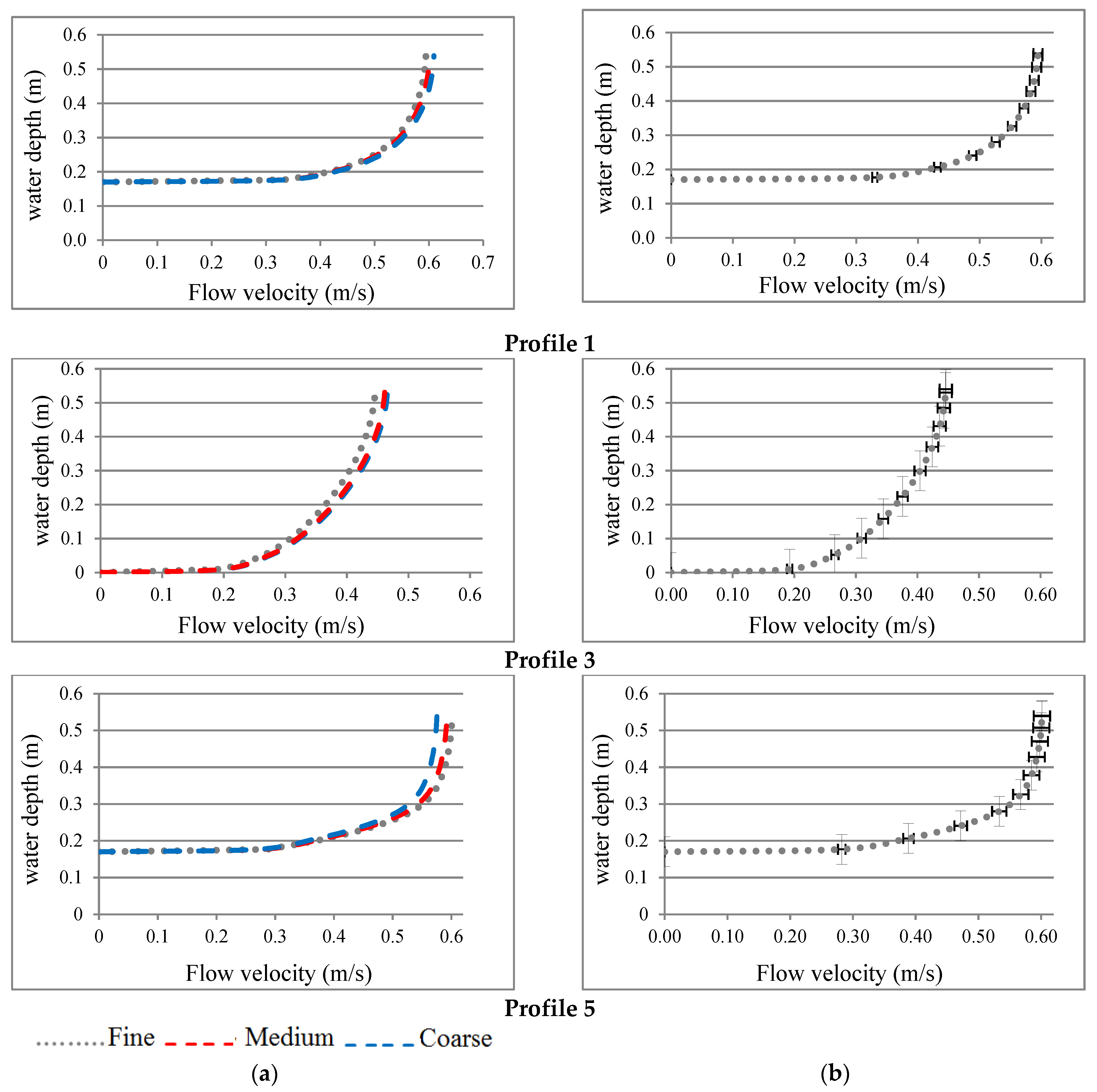
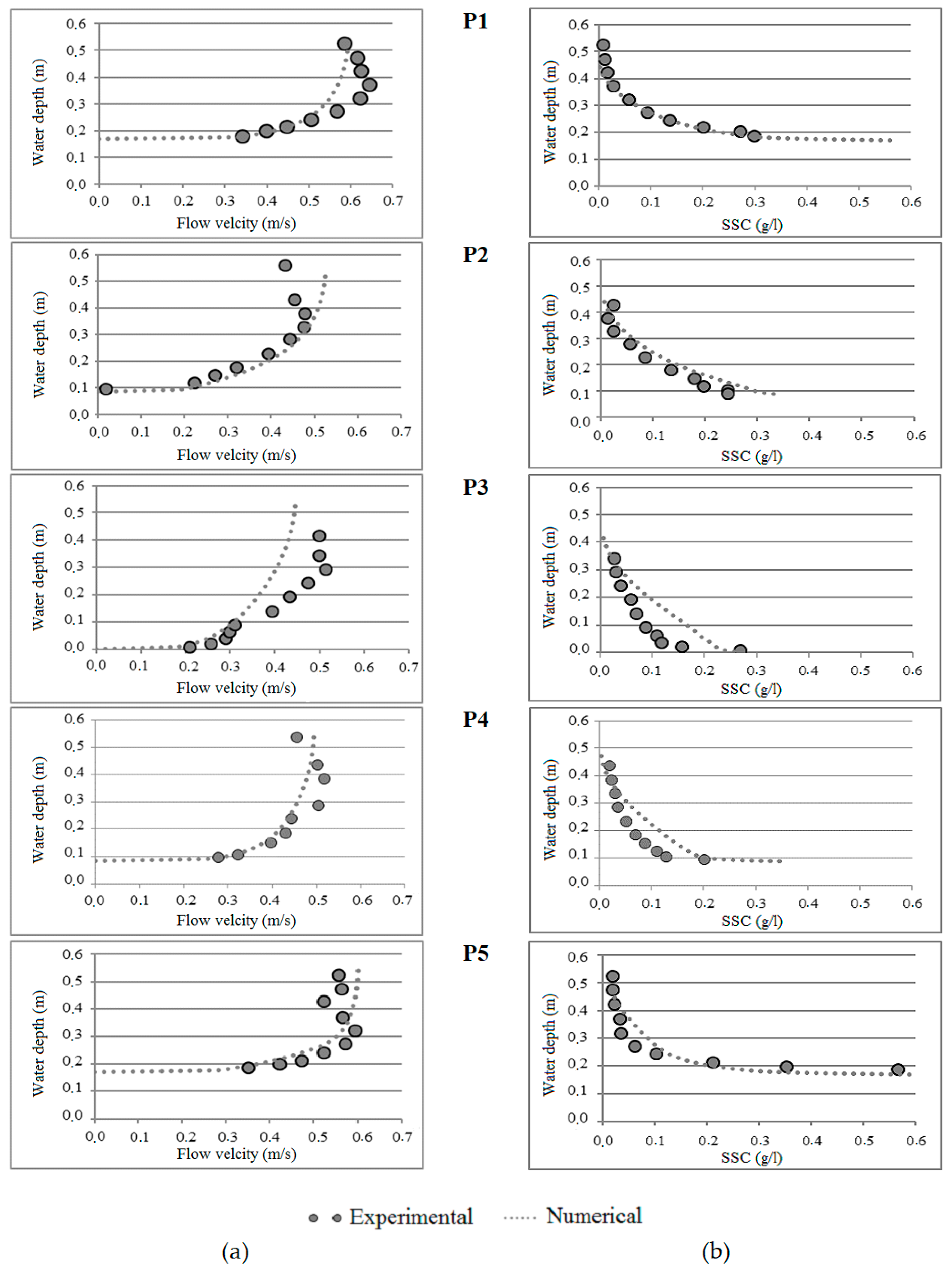
3.1. Verification and Validation of Coupled Model

The verification and the validation of the coupled hydrodynamic-sedimentary model were performed using the [14] trench tests. This procedure was performed by comparing the numerical solution of the fluid flow velocity and the suspended sediment concentration to the experimental data provided by [14] at different gauge positions. The geometry and dimensions of the selected trench are shown in Figure 2. The values of the main parameters used for the tested configuration are given in

Table 1. Main characteristics of the selected channel and sediment.

Sediment size	d50 (m)	0.00016
Bed roughness	Ks (m)	0.025
Upstream flow depth	h0 (m)	0.40
Average upstream velocity	u0 (m/s)	0.50
Density of sediment	${\rho }_s$ (kg/m3)	2650
Density of water	$\rho$ (kg/ m3)	998.2

.

The same boundary conditions were used to perform the verification and validation tests (see Figure 3): the velocity inlet condition is applied on the trench inlet, and the pressure outlet condition is applied on the outlet boundary. The trench bottom was considered as a wall with roughness height. The sides and top of the trench were modeled as a symmetry plane condition.

Note that, the verification of the sensitivity of the coupled hydrodynamic-sedimentary models to the mesh quality is an indispensable step in this work. The objective of this verification is to generate an optimal mesh that is sufficient to ensure high accuracy of the numerical solution while minimizing the calculation time. It should be noted that the numerical solution must be independent of the mesh quality.

Hence, based on the International Towing Tank Conference (ITTC) [21] recommendations, three mesh qualities were tested: fine (41,600 elements), medium (30,550 elements), and coarse (22,000 elements). Note that the three mesh qualities were generated with respect to the y+ value near the wall (the bottom). The numerical uncertainly due to the quality of the mesh was estimated based on the verification methodology proposed by [22].

This methodology consists of initially verifying the value of the constant refinement ratio r_k. The value of this constant should be about $\sqrt{2}$ between medium/fine ($r_{21}=h_{coarse}/h_{medium}$) and coarse/medium ($r_{32}=h_{medium}/h_{fine}$) mesh, and greater than 1.3 for the global ratio r between the coarse and the fine mesh ($r=h_{coarse}/h_{fine}$). h, is the representative cell that corresponds to the average cell volume ($h=\frac{1}{N_{elements}}{\displaystyle \sum }_{i=1}^{N_{elements}}\Delta V_i$). For this study, the values of these parameters are summarized in

Table 2. Grid convergence study parameters.

	Fine	Medium	Coarse
Grid number (103)	41.60	30.55	22.00
h (10−2 m)	1.32	2.18	3.33
rk	1.53		1.65

.

The solution deviations between the fine-medium (ϵ₂₁ = S₂ − S₁) and the medium-coarse (ϵ₂₃ = S₃ − S₂) mesh are computed for the flow velocity and the suspended sediment concentration (SSC). Here, the solution is represented by a profile which enables the computation of this deviation for each point of this profile (10 points). Hence, solution deviations take the form of a vector. Three profiles of the trench (inlet, center, and outlet) were considered to study the influence of the mesh on the numerical solution.

Using the deviation values computed above, the convergence ratio R_k = ϵ₃₂/ϵ₂₁ was calculated for each profile and at each point to characterize the convergence quality:

–

0 < R_k < 1 corresponds to monotonic convergence

–

R_k < 0 corresponds to oscillatory convergence

–

R_k > 1 corresponds to monotonic divergence

Based on this ratio, we find that for the flow velocity, 100% of the points of the profile have a monotonic convergence. For Profile 3, the convergence is monotonic for 90% of the points, and 10% are oscillatory. However, for Profile 5 only 70% are monotonically converged, while 30% are oscillatory. Concerning the SSC, the convergence is monotonic for 80% of points of the first profile, while 100% of the points of Profile 3 and 5 are monotonic. As a consequence, we can consider that the grid convergence criterion is verified for both the flow velocity and the SSC.

To estimate the numerical uncertainty, the fine-grid convergence index $GC{I}_{fine}^{21}$ was computed using the expression:

$$GC{I}_{fine}^{21}=\frac{1.25e_a^{21}}{r_{21}^p-1}100$$

(18)

where, $e_a^{21}$ and $P_k$ are the relative error and the order of accuracy, respectively. These two parameters are computed as follows:

$$e_a^{21}=\frac{\left|S_1-S_2\right|}{S_1}$$

(19)

And

$$P_k=\frac{ln\left({ϵ}_{32}/{ϵ}_{21}\right)}{ln\left(r_k\right)}$$

(20)

The sensitivity study shows a slight influence of the mesh refinement on the numerical solution. This is can be observed clearly from Figure 4 and Figure 5 which represent the flow velocity and the SSC profiles, respectively, at locations P1, P3 and P5 of the trench. The slight deviation noted between the three numerical solutions is principally due to the respect of the y+ value. Note that, for each tested mesh the y+ value is fixed to 50. From the same figures (right side), it can also be observed that the convergence index for the longitudinal flow velocity increases when approaching the free surface especially at the trench outlet (Profile 5), where the maximum convergence index is 1.48%, 2.00%, and 2.59% for Profiles 1, 3 and 5, respectively. This deviation increase close to the free surface can be explained by the fact that the finer the mesh at the water–air interface, the better the resolution of the free surface deformation; consequently, the flow velocity is impacted close to this interface.

For the SSC, the convergence index is larger than the flow velocity index, where the maximum convergence index is 4.01%, 1.64%, and 4.68% for profiles 1, 3 and 5, respectively, noted close to the bottom. Hence, it can be concluded that the numerical model used for this investigation accurately estimates the SSC in the fluid domain. However, this model is very sensitive to the mesh variation close to the bottom. As a consequence, the fine mesh was used to conduct the validation tests and the corresponding numerical settings were selected to perform the studied cases presented in the second part of this work. This sensitivity is likely due to the value of boundary condition C_a which depends on the empirical value of $\alpha$. This value must be calibrated for our case study.

The methodology used to verify the sensitivity of the numerical solution to the mesh quality around the ship (hull-propellers-rudders) was detailed in previous studies by [23,24]. Hence, verification and validation tests are not reproduced in the present investigation; however, the same settings used in previous studies were applied, except for close to the channel bottom where the mesh refinement settings are based on the results of the mesh sensitivity study detailed above.

To validate the numerical model used for this investigation, the vertical variation of the longitudinal flow velocity and the SSC computed in five different locations of the trench (inlet, two slopes, center, and outlet of the trench) were compared to the measured data provided by [14] (see Figure 6).

Generally, the computed flow velocity and SSC profiles have the same trend as numerical results obtained by the Van Rijn model. A good agreement between the computed results and measured data was observed, where, at the inlet zone of the trench (Profile 1), the relative error of the flow velocity does not exceed 8% with a maximum that is observed at the middle of the water column. The relative error of the flow velocity was less than 4% with a maximum that is observed near the free surface at the decelerated (Profile 2), accelerated (profile 4), and outlet (profile 5) zones of the trench. As shown in Figure 4, the larger deviation of the flow velocity between the numerical model results and measurements is noted at the center of the trench (profile 3), where the relative error is about 14%. The same results were also noted previously by [14]. The main reason for the observed discrepancy is the forcing by the non-established flow at the inlet zone with an application of the constant profile of the flow velocity at the inlet boundary condition, which affects the other profiles. To avoid this problem, Van Rijn proposed the use of the experimental profile of the flow velocity at the inlet trench as an upstream boundary condition.

For the sediment concentration, a very good agreement is noted in the inlet, the decelerated, and the outlet zones, with the relative error being less than 3%. The concentration is estimated closely in both the bed and the free surface levels. However, in the center and accelerated zones, a larger discrepancy is observed especially at the trench bed. This discrepancy can be explained by the initial concentration applied on the trench bed or is likely due to the low diffusivity computed near the bed.

Finally, we can conclude that the developed numerical model produces an acceptable estimation of both the flow velocity field and the suspended sediment concentration; hence, the numerical model is considered verified and validated.

3.2. Scaling Method Validation

Based on the similitude theory, the studied trench domain was scaled to 1/25. The sediment diameter was also scaled based on the formula given in Section 2.3 (sediment scaling method). Only the inlet boundary condition was modified by the scale change. To compare the numerical solution with measurements, the values for the measured flow velocity at different positions of the trench on one hand scaled. On the other hand, the SSC values were not scaled.

Figure 7 shows the flow velocity and the SSC profiles at five positions of the trench. By comparing the profiles, we observe the same behavior as in the full model. Generally, there is a good agreement between the computed solution and measurements. A weak change in the numerical solution of the flow velocity is observed at the inlet, decelerate and center zones of the trench, while the change in the others zones is non-significant. For the SSC, curves representing the numerical solution of the reduced model have the same trend as the full model, and the deviation between the full and reduced model can be considered non-significant. The numerical solution provides closer agreement, especially at the inlet, decelerate and outlet zones. Based on these results, it can be considered that the scaling method selected for this investigation is reliable and generates reasonable results.

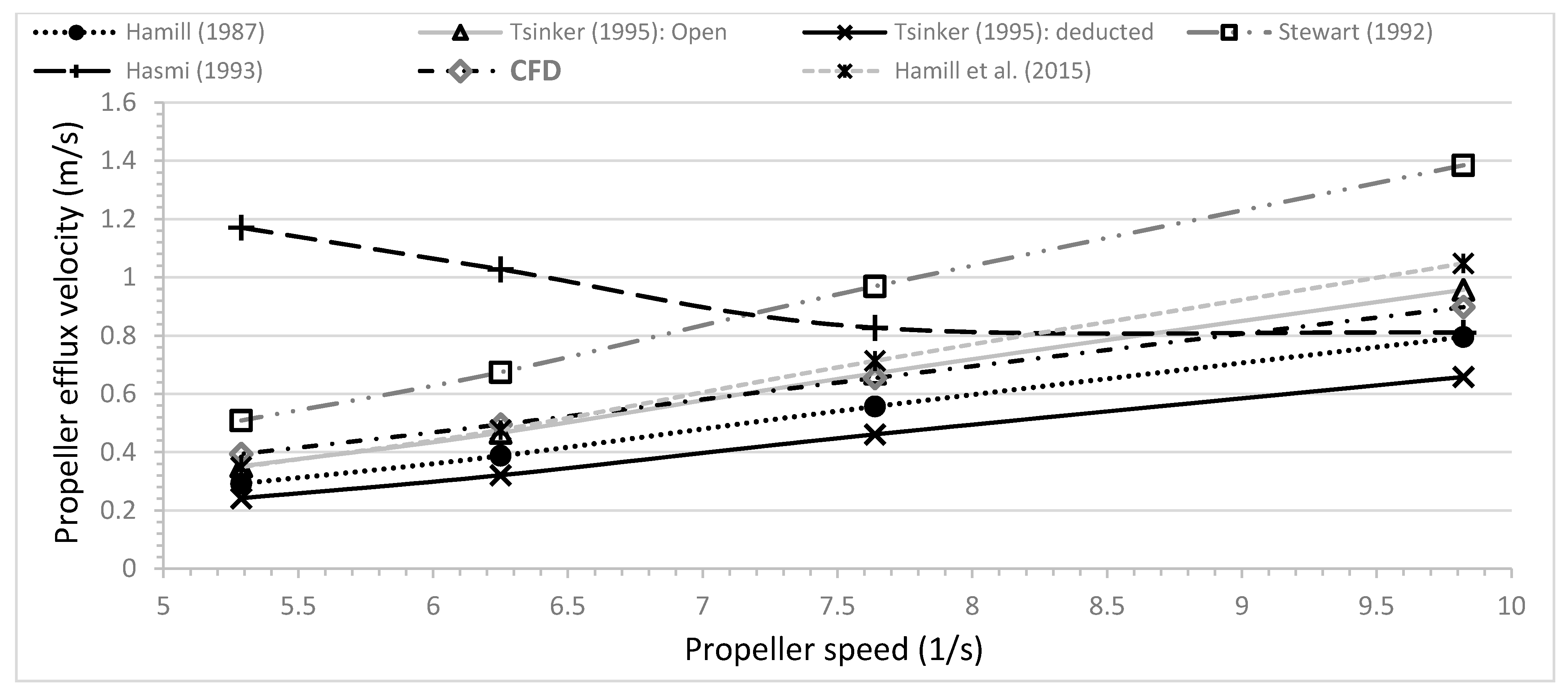
3.3. Verification of the Propeller Jet Velocity

In this section, the propeller jet velocity ($V_0$) was verified using analytical and empirical formulations from literature. In fact, several studies involved estimations of the propeller jet velocity and its impact on waterway bottoms. These works utilize a mathematical formulation based on the [3] equation (Equation (19) which is derived from the axial momentum theory.

$$V_0=1.59n{D}_p\sqrt{C_T}$$

(21)

where, n is the turning rate of the propeller, $D_p$ is the propeller diameter and $C_T$ is the thrust coefficient. In PIANC [25] this equation was generalized by replacing the value of 1.59 with a coefficient α for which other others proposed different values or formulas. Among the various formulations proposed, we selected only five formulations that are compatible with our configurations (see

Table 3. The $\alpha$ coefficient by authors.

Authors	Coefficient “α”	Nomenclature
[3]	$\alpha =1.59$	-
[1]	$\alpha =1.33$	-
[4]	$\alpha =D_p^{-0.0686}{\left(\frac{P}{D_p}\right)}^{1.519}{\beta }^{0.323}$	P: is the propeller’s pitch $\beta$: is the blade area ratio
[5]	$\alpha =C_T^{-1.79}{\left(\frac{D_p}{D_h}\right)}^{-0.403}{\beta }^{0.744}$	$D_h$: is the propeller hub diameter
[6]	$\alpha =1.33$ (free propeller) $\alpha =1.10$ (ducted propeller)	-

).

The propeller efflux velocity calculated using the formulations that are given above were compared to the efflux velocity obtained using the CFD simulations for several propeller speeds. To perform this comparative study, the ship’s speed was set to 0.55 m/s and the advance coefficient was varied (0.7, 0.9, 1.1, and 1.3) by varying the propeller’s speed (589, 458, 375 and 317 rpm). The used propeller’s pitch ratio is 1.635.

In Figure 8, the propeller efflux velocity using several formulas and the CFD method is plotted as a function of propeller speed. From this figure, it can be observed that the propeller efflux velocity varies significantly from one study to another despite all the tests verifying the conditions of use of these formulas. Of note, all of the curves are nearly linear, including the CFD results. We note also that Stewart’s formula overestimates the efflux velocity, while Tsinker’s formula underestimates it. Hasmi’s formula seems to give a correct value for the efflux velocity at higher propeller speeds while at lower propeller speeds the formula overestimates the velocity. By comparing the different curves, we see that the CFD model gives average values for the efflux velocity, and the values are very close to the results obtained using Tsinker’s formula [6] for an open propeller and Hamill et al.’s formula [26]. This result confirms the ability of the CFD model to reproduce the complex flow generated by propellers.

4. Application

In this part, the developed numerical model will be used to conduct numerical investigations. These investigations concern the estimation of the inland traffic impact on the seabed shear stress and therefore sediments suspension. The following sections give more information on the ship design, the channel geometry, the boundary conditions and different tested configurations.

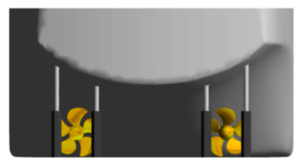
4.1. Ship’s Description

An inland container ship was used as the basis for this study (see Figure 9). The dimensions of the ship’s hull are given in

Table 4. Main characteristics of the ship’s hull.

	Full Scale Model	Scaled Model (1/25)
Length (LPP)	135 m	5.4 m
Beam (B)	11.4 m	0.456 m
Draught (T)	2.5 m	0.1 m
Block coefficient (CB)	0.899	0.899
Wetted surface (WS)	2104.8 m2	3.367 m2
Cross area of ship (CS)	34.114 m2	0.0545 m2

. The propulsive system is equipped with two similar propellers (type VP1304) with five blades. The main characteristics of the propellers are presented in

Table 5. Propulsive system characteristics.

Propeller Data
Type	Fixed Pitch
Number of propellers	np	2
Number of blades	z	5
Propeller Diameter	DP	0.08 m
Hub diameter ratio	Dh/DP	0.03 m
Pich at r/R = 0.7	P0.7	0.130 m
Skew angle	$\theta$	18.8°
Rotation direction: Port propeller Starboard Propeller		Right-handed Left-handed

. The steering system of this ship is controlled by four rudders (type Schilling), two of which are located behind each propeller (see Figure 10). All tested cases were performed at a 1/25 scale by considering the Froude scaling law.

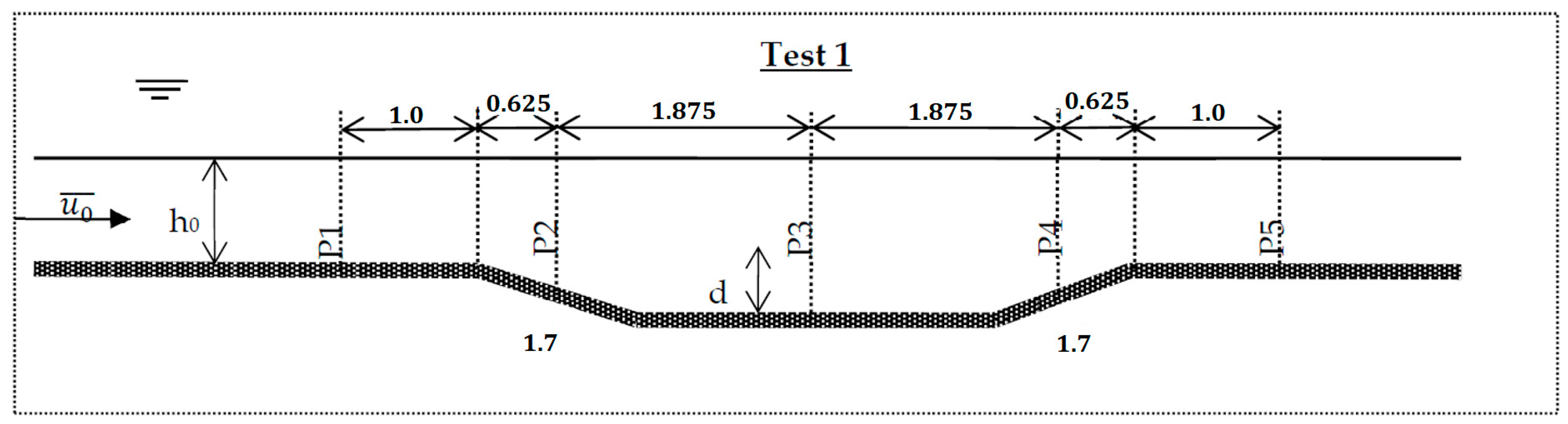
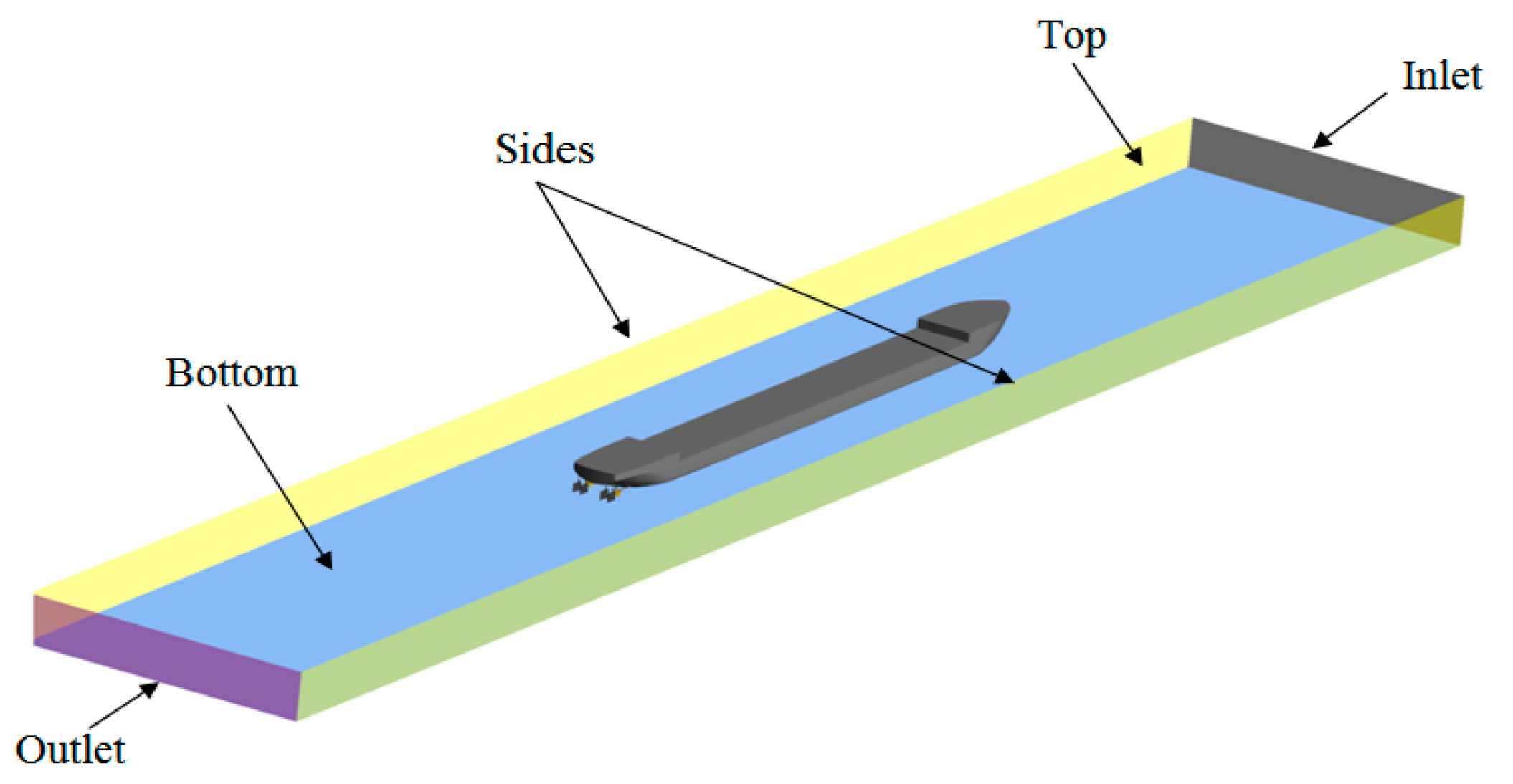
4.2. Channel Configurations and Corresponding Boundary Conditions

The channel form and boundary conditions used to carry out these investigations were illustrated in Figure 11 and listed in

Table 6. Boundary conditions.

Inlet	Pressure Inlet	Free Surface Level with x-Velocity (Ship’s Velocity)
Outlet	Pressure outlet	Specified Free Surface Level
Ship hull	Wall	No Slip & Wall Roughness (Default)
Bottom wall	Moving wall	No Slip & Motion: x-velocity & Wall Roughness (0.025)
Sides and top	Symmetry	Default

. The channel long corresponds to 3.5 times the length of the ship, where the inlet is located at one ship’s length while the outlet boundary is located at 1.5 ship’s length. The channel width corresponds to five times the ship width. The same conditions were used for all simulated tests. No slopes were considered on the channel sides.

As mentioned above, the aim of these investigations is to study the impact of the ship passage on the sediment suspension. Hence, several scenarios were simulated by varying four parameters: depth to draught ratio (h/T), ship speed, ship advance ratio, and sediment size. The evaluated configurations are summarized in

Table 7. Evaluated parameters: ship speed Vs (m/s), depth to draught ratio (h/T), advance ratio (J), and sediment size (m).

	h/T = 1.2	h/T = 1.5	h/T = 2.0	h/T = 3.0
J = 1.3	0.55 (m/s)/d50 = 1.6 × 10−6 m	X	X	X
J = 1.1	0.55 (m/s)/d50 = 1.6 × 10−6 m	0.55 (m/s)/d50 = 1.6 × 10−6 m	0.55 (m/s)/d50 = 1.6 × 10−6 m	0.55 (m/s)/d50 = 1.6 × 10−6 m
	/d50: 1/1.6/2.4/3 × (10−6 m)
J = 0.9	0.55 (m/s)/d50 = 1.6 × 10−6 m	X	X	X
J = 0.7	0.55 (m/s)/d50 = 1.6 × 10−6 m	X	X	X

.

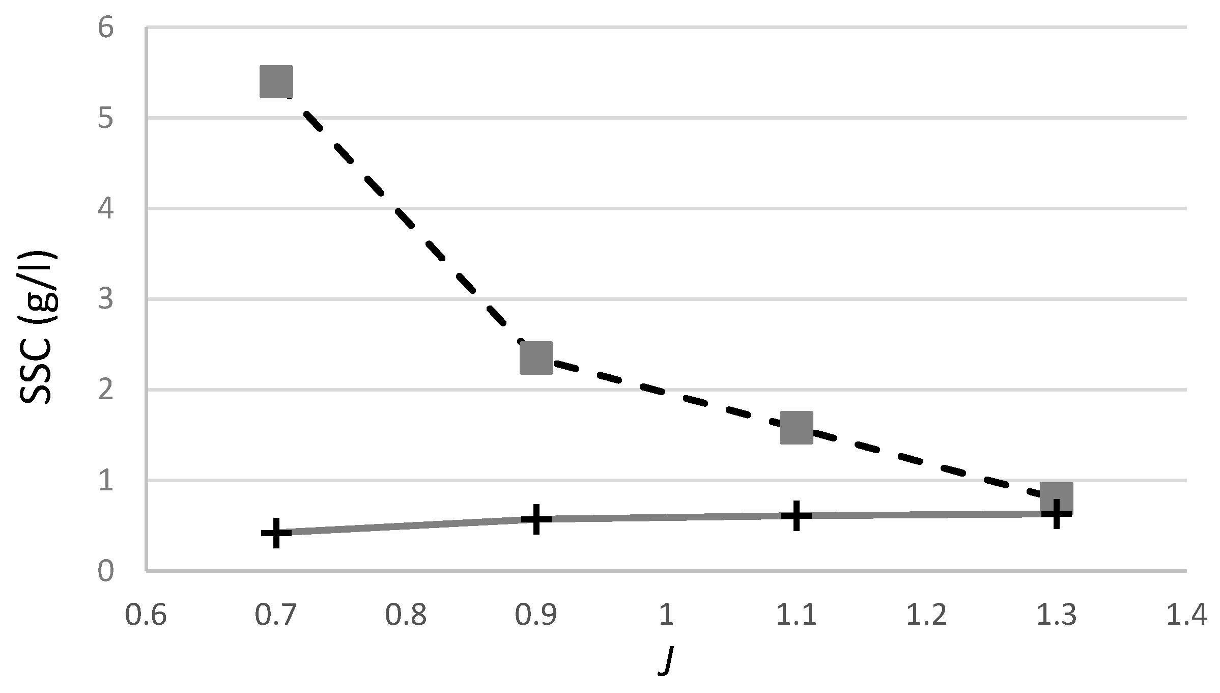
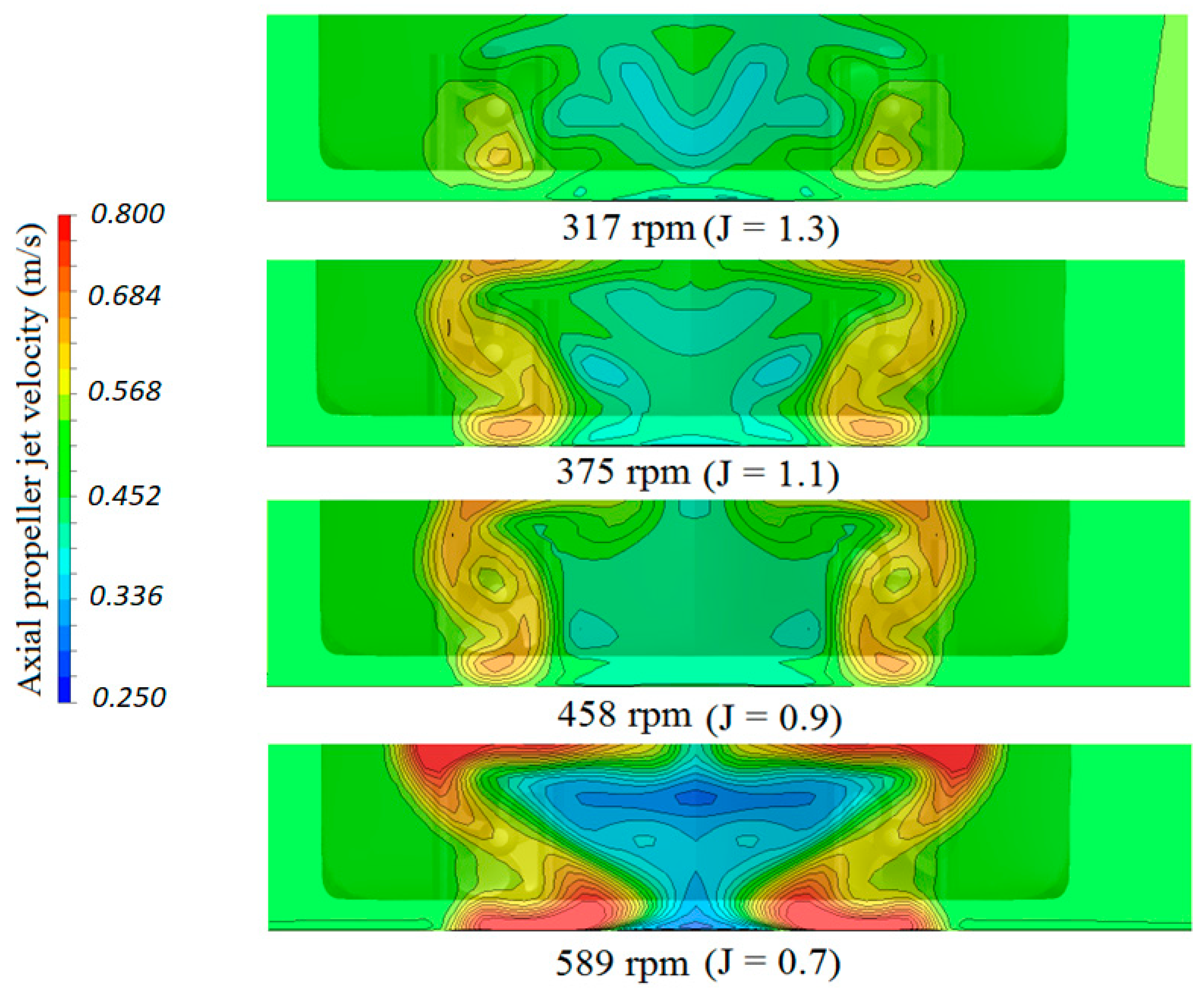
4.3. Propellers Effect on the Sediment Suspension

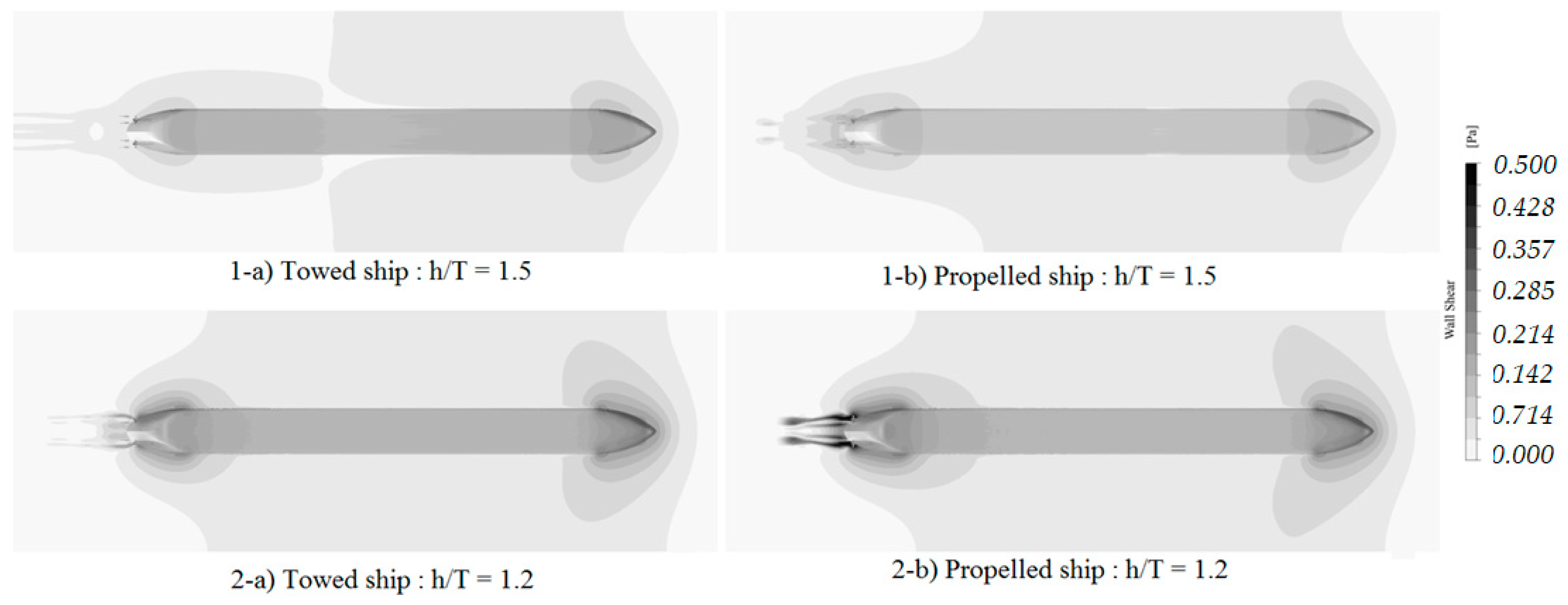
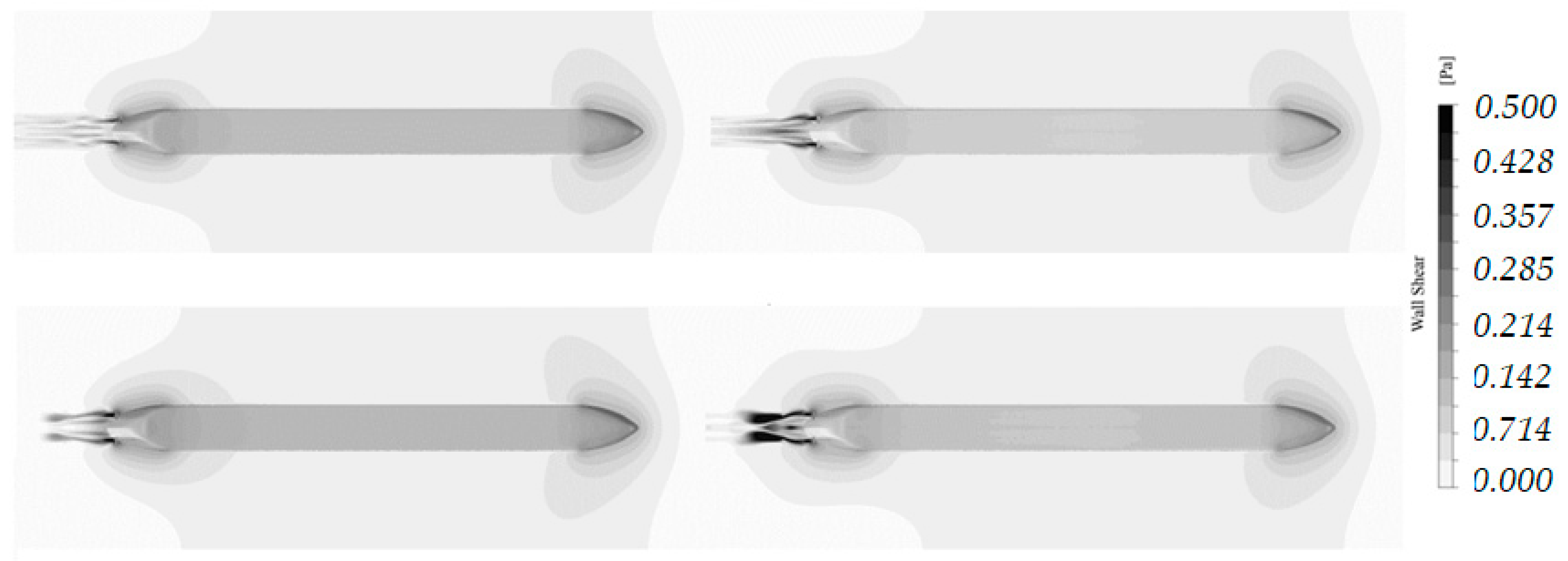
4.3.1. Propeller Jet Effect on the Bed Shear Stress

As mentioned in the Introduction section, the estimation of the suspended sediments during the ship passage is often characterized by the propeller’s efflux velocity. In confined water, the effect of the return current that is generated by the hull can also be significant. Hence, we investigated the influence of the return current caused by the hull and the combined effect of the hull and propeller jet on the bottom erosion. To carry out this comparative study, we calculated the bed shear stress by simulating the flow around a towed and propelled ship model for two different h/T ratios (1.2 and 1.5) which correspond to shallow and confined water, respectively. The ship’s speed was set to 0.55 m/s, while the propeller speed was set to 375 rpm (J = 1.1). First, we assessed the effect of the return current generated by the towed hull motion on the bed shear stress. Then, the propellers were activated to assess the additional shear stress applied on the bottom by the propulsive system. Figure 12 illustrates the iso-contours of the shear stress on the channel bed.

Figure 12 shows clearly that for both h/T ratios the bed shear stress is concentrated on the bow and the stern of the ship. For the case of a towed ship, it can be seen that the bed shear stress and the impacted area are more significant at the ship’s bow than at the ship’s stern. It can also be observed that the closer the bed, the larger the shear stress and also the impacted area. This is due primarily to the return current generated by the ship’s motion ([24]). Note that the return current increases with decreasing h/T ratio (confined water).

By activating the propellers, the shear stress in the shallow water case increases slightly at the ship’s stern, still less significantly than at the ship’s bow. However, in confined water, the shear stress increases significantly. We also note that the impacted area at the ship’s stern is slightly affected by the propeller jet in shallow water, while it is unchanged at the ship’s bow. In confined water, the propeller jet effect becomes very significant especially behind propellers and, consequently, the impacted area is larger. Contrary to the shallow water case, in confined water, the maximum bed shear stress at the ship’s bow is slightly impacted while the impacted region is larger. The observations noted here are more easily seen by the graphs shown in Figure 13. In this figure, the Suspended Sediment Concentration (SSC) generated by the ship motion (towed and propelled) in shallow and confined waters was plotted under the ship along a longitudinal line passing by the propeller’s axis. The SSC was taken at the height of 0.015 m from the channel bed.

From these graphs, it can be seen that the SSC induced by the ship motion is almost unchanged at the ship’s bow for all configurations (towed and propelled ship). This leads us to the conclusion that, for both h/T ratios, the shear stress generated at the ship’s bow is mostly caused by the return current and that the propeller effect is negligible; However, for the propelled ship, we can also observe that in shallow water the computed SSC at ship’s bow is approximately 0.4 g/L which corresponds to double the SSC generated at the ship’s stern. In confined water the situation is inversed, where the value of the SSC generated at the ship’s stern becomes more significant, which is about 1.54 g/L while at the ship’s bow the maximum value of the SSC is about 0.82 g/L. This observation allows us to note that the effect of propellers is significant only when the ship is navigating in a confined configuration.

From the same figures, we observe that the quantity of the SSC computed under the ship increases slightly in confined water which can be related to the accelerated flow induced by the combined effect of the hull and propellers. However, for a given h/T ratio the SSC variation is almost unchanged except close to the ship’s stern where the SSC starts increasing due to the propeller’s influx flow.

To more precisely identify the effect of the propulsive system, a series of simulations was carried out by varying the propellers’ speed. Four speeds were considered 589, 458, 375 and 317 rpm which correspond to an advance ratio of 0.7, 0.9, 1.1 and 1.3, respectively. The confined water configuration (h/T = 1.2) was selected to perform these simulations, and the ship’s speed was fixed to 0.55 m/s. Figure 14 shows the bed shear stress as a function of the propellers’ speed. From this figure, we can see that the propellers have a significant effect, particularly at the ship’s stern. This variation of the bed shear stress is typical because the shear stress increases with increasing propeller speed. However, to quantify the effect that the propellers’ speed variation induces on the SSC, the latter was plotted along the line passing through the center of a propeller and located at a height of 0.015 from the bottom (see Figure 15). It can be seen that, by increasing the propellers’ speed, the impacted area and the SSC variation at the ship’s bow was negligible while the impacted area as well as the SSC at the ship’s stern increase considerably. At low propeller speeds, the maximum value of the SSC was about 0.82 g/L, while at higher speeds the maximum SSC value was about 5.3 g/L, which corresponds to an amplification factor of 6.6. The amplification relative to the propellers’ speeds of 375 and 458 rpm were approximately 2 and 3, respectively. By plotting the maximum SSC at the bow and stern regions according to propeller speed (see Figure 16), it can be deduced that the SSC variation at the ship’s bow is almost constant, while at the ship’s stern the SSC variation follows the function given in Equation (22).

$$SSC\left(J\right)=1.85J^{-2.97}$$

(22)

To well illustrate the effect of the propulsive system on the SSC, the contours of the axial velocity of the efflux jet in the transversal plane located at 0.25 m behind the ship’s stern were plotted in Figure 17. The figure shows that for low propeller speeds the vortices are larger and the intensity generated by propeller operation is weak and dissipates before touching the bottom. As the propellers’ speed increased, the vortices are larger and their velocity is more intense, especially close to the bottom. This behavior can explain why the amplification factor noted for higher propeller speeds is despite that, the step of variation of the advance coefficient is the same (0.2).

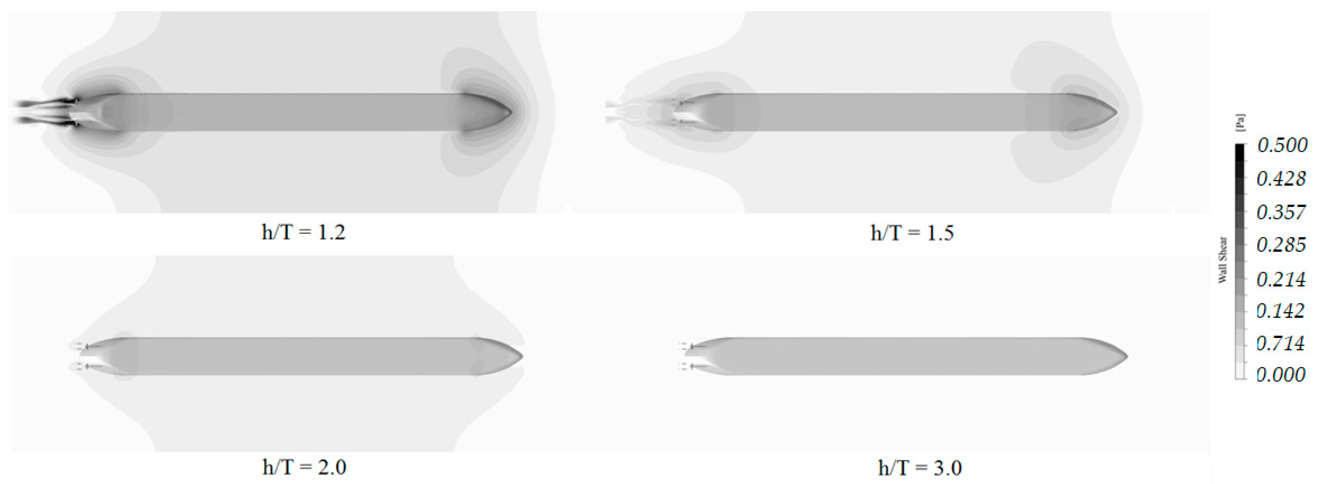
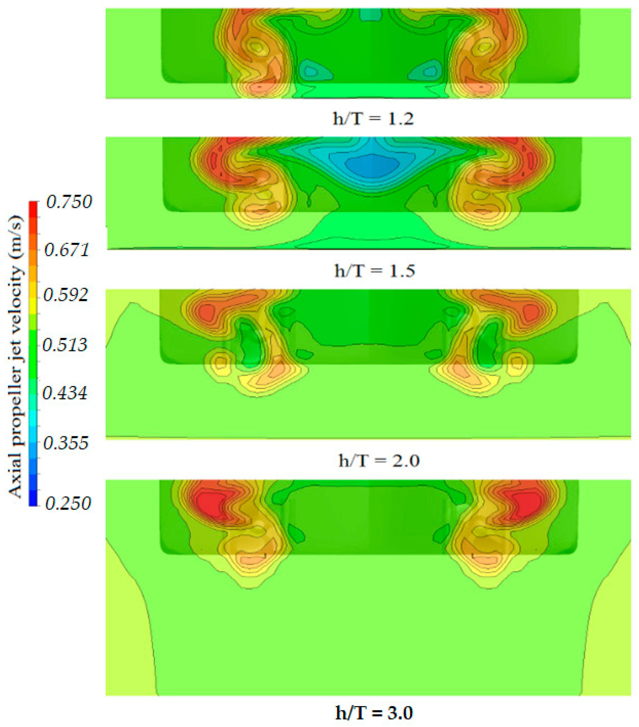
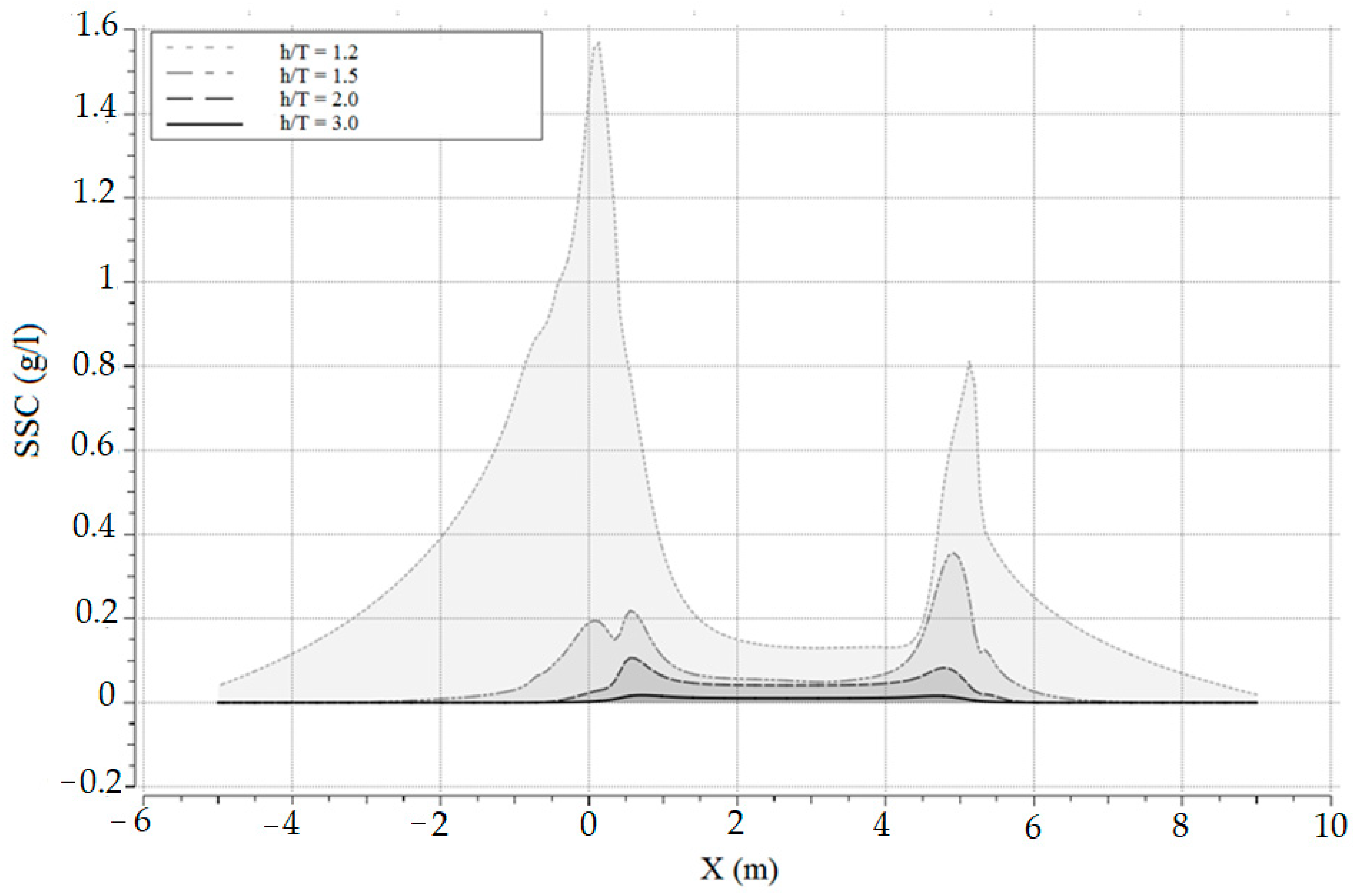
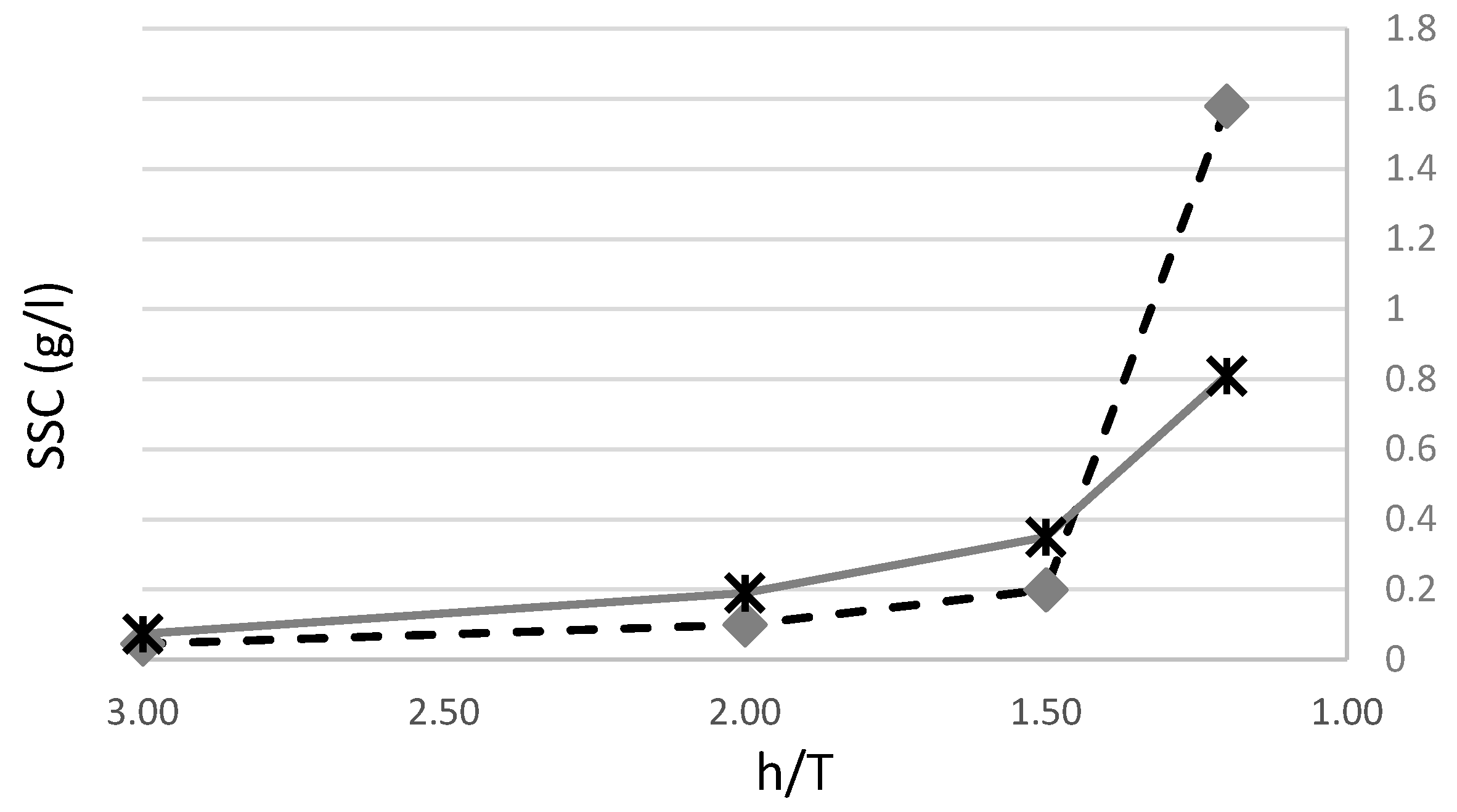
4.3.2. Confinement Effect on the Concentration of the Suspended Sediments in Inland Waterway

The confinement of the inland waterway is considered to be one of the major factors that considerably influences the suspension of sediments. In fact, the closer the ship is to the waterway bottom, the greater the suspension of the sediment. This phenomenon can be expressed by the increase of the return currents intensity caused by the reduction of the fluid passage section under the hull, and also by the propeller efflux jet generated by the propulsive system close to the bottom. To study the influence of the confinement on the suspended sediment, four simulations were carried out by varying the h/T ratio, where each h/T value corresponds to an inland waterway type (h/T = 1.2, confined water; h/T = 1.5, shallow water; h/T = 2.0 medium deep water; and h/T = 3.0, deep water). Using a ship speed of 0.55 m/s, a ship draught of 0.1 m, and a propeller turning rate of 375 rpm (J = 1.1), the depth Froude number for each channel configuration was calculated as follows: 0.101 for confined water, 0.090 for shallow water, 0.078 for medium deep water, and 0.064 for deep water.

Figure 18 shows the bed shear stress as a function of the h/T ratio. It can be seen that the propeller and hull effect is felt by the bed only in confined, shallow and medium deep waters. However, this effect is more visible when the ship is navigating in confined and shallows water, where the computed shear stress value in confined water that is 3.5 times higher compared to that for shallow water and 12 times higher than that for medium deep water. The effect of the h/T ratio is primarily observed at the ship’s bow and the ship’s stern. In deep water, the impact of the ship passage and its propulsive system is non-significant, and the numerical results show that the hull effect dominates over the propeller effect.

To understand the effect of the confinement on the bed shear stress, the axial velocity of the propeller efflux is plotted on the transversal plane located at 0.25 m behind the ship’s stern (see Figure 19). The results clearly show that the propeller efflux jet significantly impacts the bottom only in confined water. The impact is weak in shallow water, while in medium deep and deep water, the turbulence generated by the propeller jet dissipates far from the bottom, and only the returned currents generated by the ship’s hull affect the concentration of the suspended sediment.

The longitudinal distribution of the SSC along the channel (the line passes through the propeller center and is located at 0.015 m above the bottom) was illustrated in Figure 20. From this figure, the same conclusion can be made as for the observation cited above, which is that the SSC for deep water is non-significant and the only effect felt is that of the hull (under the hull) while, in medium deep and shallow water, the SSC increases at the bow and the stern of the ship, with a larger increase at the ship’s bow. In confined water the tendency is reversing; the SSC increases significantly under the ship with a greater effect at the ship’s stern. At the ship’s bow, the maximum SSC value is 2.3 times larger than in shallow water; however, the SSC at the ship’s stern is about 1.52 g/L which corresponds to nearly double the SSC at the ship’s bow and seven times the SSC at the ship’s stern in shallow water (see Figure 21). These observations reinforce the hypothesis that the propulsion effect is only important if the ship is navigating in a confined environment (h/T < 1.3) and that the effect of the returned currents is dominant in the others configurations. Hence, it is indispensable to include the hull effect in numerical models to estimate accurately the concentration of the suspended sediments caused by ship traffic.

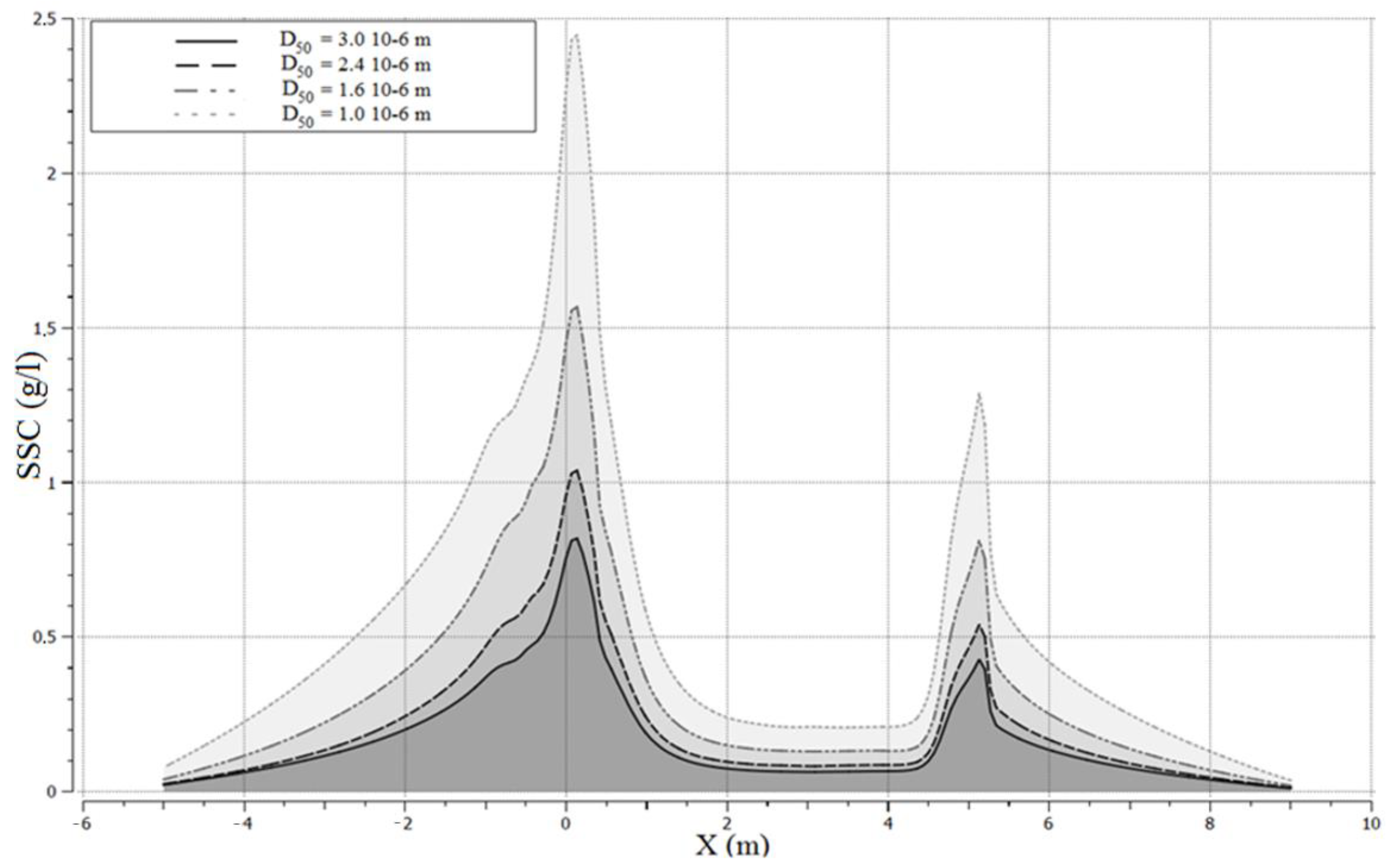
4.3.3. Influence of the Sediment Size on the SSC

The last parameter studied in this work is the influence of the sediment size on the SSC during the ship’s passage. For this, four scaled sediment sizes were tested in confined water (h/T = 1.2). The ship’s speed was set to 0.55 m/s and the propeller turning rate was set to 375 rpm (J = 1.1). The sediment size was scaled based on the Shields parameter equation. The values of the scaled sediment sizes used were 1.0 × 10⁻⁶, 1.6 × 10⁻⁶, 2.4 × 10⁻⁶, and 3.0 × 10⁻⁶ m (which correspond to 0.0864 × 10⁻³, 0.138 × 10⁻³, 0.207 × 10⁻³ and 0.260 × 10⁻³ m in the full model). The computed SSC was plotted as a 3D cloud in Figure 22. This representation allows us to see that, how for the same bed shear stress, the radius of the area that is impacted by the ship passage as well as the concentration of suspended sediment that is influenced by the sediment size. From this illustration, we can see clearly that the sediment size significantly influences the SSC. In fact, by reducing the sediment size, the cloud representing the SSC is denser around the ship, especially at the stern region. This behavior is physical because the critical bed shear stress (see the formulation of Yalin 1977) depends on the sediment diameter d₅₀.

The SSC distribution along the line passing through the propeller center and located at 0.015 m above the bottom was plotted in Figure 23 for the four sediment sizes. We note that the SSC distribution follows the same trend as in previous tests, where the most affected areas were located at the ship’s bow and the ship’s stern. The computed SSC at the ship’s stern is approximately double the value of the SSC at the bow. We also note that by reducing the sediment size, the SSC trend, as well as the SSC ratio between the ship’s stern and the ship’s bow, remains the same, while the profile is amplified. This finding is very interesting, especially to model the suspended sediment due to the ship traffic using models based on shallow water equations where the profile of the SSC can be reproduced and controlled by a simple coefficient depending on the sediment size.

To determine the latter coefficients, the maximum SSC value at the bow and stern regions according to sediment size was drawn in Figure 24. By fitting these curves, we deduced that the variation of the maximum SSC is following Equation (23). The coefficients a and b depend on the ship’s region, where a = −1.52 and b = 1.2 at the ship’s bow while a = 2.47 and b = −1.016 at the ship’s stern.

$$SSC\left(d_{50}\right)=a{d_{50}}^{-b}$$

(23)

5. Conclusions

In the first part of the work, a coupling between a hydrodynamic model (CFD) and a sedimentary transport model was performed. The finite volume method was used to solve the complete Navier–Stokes equations. The sedimentary transport model based on the diffusion convection equation was implemented, verified and validated. The verification included a study of the sensitivity of the CFD model to the quality of the mesh close to the bottom; hence, three mesh qualities were tested. The optimal mesh quality was used to carry out the validation tests and the studied cases.

The validation of the CFD-sedimentary coupling model was performed using measurements carried out by [14]. The first comparisons of this work showed overall a good agreement between the numerical and experimental results for the real model like on the scaled model. The source of the deviation between the numerical solution and measurements which was caused by the velocity profile applied at the inlet of the trench was also discussed.

Based on the obtained results, the coupled CFD-sedimentary model was verified and validated. This leads us to consider the model reliable and accurate for our investigation. The mesh quality close to the bottom as well as the numerical settings were utilized for the remaining modeling activities and applications under this work.

In the second part of this work, the effect of the inland navigation on the sediment suspension was simulated and discussed by varying different parameters. First, the propeller’s efflux velocity obtained by the CFD method was compared using an empirical formula. This comparison allows us to conclude that the results obtained by the CFD method are in the same range as the empirical formulas results. Secondly, the investigations were started by showing the effect of the consideration of the propulsive system. The SSC generated by a towed ship was compared to the SSC induced by propelled ship. The conclusion of this comparison showed that the SSC caused by a propelled ship passage is 3.6 times more than a towed ship (essentially at the ship’s stern).

This study was subsequently enriched by investigating the influence of propeller turning speed, the h/T ratio and the sediment size. The conclusions of these investigations were summarized below:

• The influence of the propulsive system is significant only in shallow and confined waters. In medium and deep water, the propulsive system has not a great effect.
• The h/T ratio is the parameter that has the most influence on the SSC. This parameter is also considered as an essential parameter on which the other parameters strongly depend.
• The redius of the impacted area and the quantity of the SSC depend strongly on the sediment size. Where, the smaller the sediment size, the larger the SSC quantity and impacted area.

The results of this study helped us to understand the effect of inland traffic on the environment of navigation. The results of this study allowed also us to propose simplified formulations in order to represent the variation of the maximum SSC variation at the bow and stern of ships according to parameters cited above. The conclusion of this study can also be used to improve the engineering methods and the shallow water models basing on the Saint-Venant equations.

References

1. Hamill, G.A. Characteristics of the Screw Wash of Manoeuvring Ship and the Resulting Bed Scour. Ph.D. Thesis, Queen’s University of Belfast, Northern Ireland, UK, 1987. [Google Scholar]
2. Gaythwaite, J.W. Design of Marine Facilities for the Berthing, Mooring, and Repair of Vessels; American Society of Civil Engineers (ASCE): Reston, VA, USA, 2004. [Google Scholar]
3. Fuehrer, M.; Römisch, K. Propeller jet erosion and stability criteria for bottom protection of various constructions. Bull. Perm. Int. Assoc. Navig. Congr. 1977, 58, 12. [Google Scholar]
4. Stewart, D.P.J. Characteristics of a Ship Screw Wash and the Influence of Quay Wall Proximity. Ph.D. Thesis, Queen’s University of Belfast, Northern Ireland, UK, 1992. [Google Scholar]
5. Hasmi, H.N. Erosion of a Granular Bed at a Quay wall by a Ship’s Screw Wash. Ph.D. Thesis, Queen’s University of Belfast, Northern Ireland, UK, 1993. [Google Scholar]
6. Tsinker, G.P. Marine Structures Engineering: Specialized Applications; Chapman and Hallan International Thomson Publishing Company: New York, NY, USA, 1995. [Google Scholar]
7. Smaoui, H.; Ouahsine, A.; Pham, V.; van Bang, D.P.; Sergent, P.; Hissel, P. On the sediment resuspension induced by the boat traffic: From experiment to numerical modelling. In Chapter 3, Sediment Transport; Ginsberg, S.S., Ed.; InTech: Vienna, Austria, 2011; pp. 55–70. [Google Scholar]
8. Parisi, J.; Turnbull, M.; Cooper, A.; Clarke, J. Ship-current interactions with TELEMAC. In Proceedings of the TELEMAC-MASCARET User Conference 2019, Toulouse, France, 15–17 October 2019. [Google Scholar]
9. Brovchenko, I.; Kanarska, Y.; Maderich, V.; Terletska, K. 3D non-hydrostatic modelling of bottom stability under impact of the turbulent ship propeller jet. Acta Geophys. 2007, 55, 47–55. [Google Scholar] [CrossRef]
10. Lam, W.H.; Robinson, D.J.; Hamill, G.A.; Johnston, H.T. An effective method for comparing the turbulence intensity from LDA measurements and CFD predictions within a ship propeller jet. Ocean. Eng. 2012, 52, 105–124. [Google Scholar] [CrossRef]
11. Stoschek, O.; Precht, E.; Larsen, O.; Jain, M.; Yde, L.; Ohle, N.; Strotmann, T. Sediment resuspension and seabed scour induced by ship-propeller wash. In Proceedings of the PIANC Congress, San Francisco, CA, USA, 1–5 June 2014. [Google Scholar]
12. Li, Y.; Ong, M.C.; Fuhrman, D.R. CFD investigations of scour beneath a submarine pipeline with the effect of upward seepage. Coast. Eng. 2020, 156, 103624. [Google Scholar] [CrossRef]
13. Yazdanfar, Z.; Lester, D.; Robert, D.; Setunge, S. A novel CFD-DEM upscaling method for prediction of scour under live-bed conditions. Ocean Eng. 2021, 220, 108442. [Google Scholar] [CrossRef]
14. Van Rijn, L.C. Sediment Transport, Part I: Bed Load Transport. J. Hydraul. Eng. 1984, 110, 1431–1456. [Google Scholar] [CrossRef] [Green Version]
15. Einstein, H.A. The Bed-Load Function for Sediment Transport in Open Channel Flow; U.S. Dept. of Agriculture, Soil Conservation Service: Washington, DC, USA, 1950. [Google Scholar]
16. Smith, J.D.; McLean, S.R. Spatially averaged flow over a wavy surface. J. Geophys. Res. Space Phys. 1977, 82, 1735–1746. [Google Scholar] [CrossRef]
17. Dyer, K.R. Coastal and Estuarine Sediment Dynamics; John Wiley and Sons: Chichester, UK, 1986. [Google Scholar]
18. Van Rijn, L.C. Sedimentation of Dredged Channels by Currents and Waves. J. Waterw. Port Coast. Ocean. Eng. 1986, 112, 541–559. [Google Scholar] [CrossRef]
19. Yalin, M.S. Mechanics of Sediment Transport, 2nd ed.; Pergamon Press: New York, NY, USA, 1977; 298p. [Google Scholar]
20. Robijns, T. Flow beneath Inland Navigation Vessels. Master’s Thesis, TU Delft, Delft, The Netherlands, 2014. [Google Scholar]
21. ITTC (Repport), Recommanded Procedures and Guidelines 7.5-02-05-01, Testing and Extrapolation Methods High Speed Marine Vehicles Resistance Test (Report). 2008. Available online: https://ittc.info/media/1637/75-02-05-01.pdf (accessed on 30 June 2021).
22. Celik, I.B.; Ghia, U.; Roache, P.J.; Freitas, C.J.; Coleman, H.; Raad, P.E. Procedure for Estimation and Reporting of Uncertainty Due to Discretization in CFD Applications. J. Fluids Eng. 2008, 130, 078001. [Google Scholar] [CrossRef] [Green Version]
23. Kaidi, S.; Smaoui, H.; Sergent, P. Numerical estimation of bank-propeller-hull interaction effect on ship manoeuvring using CFD method. J. Hydrodyn. 2017, 29, 154–167. [Google Scholar] [CrossRef]
24. Kaidi, S.; Smaoui, H.; Sergent, P. CFD Investigation of Mutual Interaction between Hull, Propellers, and Rudders for an Inland Container Ship in Deep, Very Deep, Shallow, and Very Shallow Waters. J. Waterw. Port Coast. Ocean. Eng. 2018, 144, 04018017. [Google Scholar] [CrossRef]
25. PIANC. Guidelines for Protecting Berthing Structures from Scour Caused by Ships; Report No. 180; The World Association for Waterborne Transportation Infrastructure: Brussels, Belgium, 2015. [Google Scholar]
26. Hamill, G.A.; Kee, C.; Ryan, D. 3D Efflux velocity characteristics of marine propeller jets. Proc. ICE Marit. Eng. 2015, 168, 62–75. [Google Scholar] [CrossRef] [Green Version]
Figure 1. Flowchart of the coupling method.
Jmse 09 00746 g001
Figure 2. Trench design and dimensions.
Jmse 09 00746 g002
Figure 3. Trench geometry and boundary conditions.
Jmse 09 00746 g003
Figure 4. Sensitivity analysis: (a) longitudinal flow velocity profile and (b) fine mesh solution with error bars of the G C I f i n e 21 .
Jmse 09 00746 g004
Figure 5. Sensitivity analysis: (a) SSC profile and (b) fine mesh solution with error bars of the G C I f i n e 21 .
Jmse 09 00746 g005
Figure 6. Comparison between numerical and experimental results of the full model: (a) flow velocity and (b) Experimental SSC [14]).
Jmse 09 00746 g006
Figure 7. Comparison between numerical and experimental results of the scaled model: (a) flow velocity and (b) SSC (Van Rijn 1984).
Jmse 09 00746 g007
Figure 8. Comparison of the propeller efflux velocity computed by CFD and by semi-empirical formulas.
Jmse 09 00746 g008
Figure 9. Ship’s hull form.
Jmse 09 00746 g009
Figure 10. Propellers and rudders positions.
Jmse 09 00746 g010
Figure 11. Channel form and applied boundary conditions.
Jmse 09 00746 g011
Figure 12. Bed shear stress for towedship (1-a,2-a) and propelled ship: (1-b,2-b) for h/T = 1.5 and 1.2 respectively.
Jmse 09 00746 g012
Figure 13. SSC along the channel (passing by the midline of propeller) for towed and propelled ship: (a) h/T = 1.5 and (b) h/T = 1.2.
Jmse 09 00746 g013
Figure 14. Bed shear stress induced by ship motion as a function of propeller speed.
Jmse 09 00746 g014
Figure 15. SSC (g/L) along the channel (passing through the propeller midline) by varying propeller speeds.
Jmse 09 00746 g015
Figure 16. Maximum SSC (g/L) variation at the ship’s stern and the ship’s bow according to ship’s advance coefficient (propeller speed).
Jmse 09 00746 g016
Figure 17. Axial propeller efflux jet velocity at the transversal plane located at 0.25 m behind the ship’s stern: propeller speed variation.
Jmse 09 00746 g017
Figure 18. Bed shear stress as a function of h/T ratio.
Jmse 09 00746 g018
Figure 19. Axial propeller efflux jet velocity at the transversal plane located at 0.25 m behind the ship’s stern: h/T ratio variation.
Jmse 09 00746 g019
Figure 20. SSC (g/L) distribution on the midline of the ship according to the h/T ratio.
Jmse 09 00746 g020
Figure 21. Maximum SSC (g/L) variation at the ship’s stern and the ship’s bow according to the h/T ratio.
Jmse 09 00746 g021
Figure 22. Volume representation of the SSC (g/L) distribution on the water according to sediment size.
Jmse 09 00746 g022
Figure 23. SSC (g/L) distribution along the line passing through the propeller center (located 0.015 m above the bottom).
Jmse 09 00746 g023
Figure 24. Maximum SSC (g/L) variation at the ship’s stern and the ship’s bow according to sediment size.
Jmse 09 00746 g024