Short Term Forecast of Container Throughput: New Variables Application for the Port of Douala

Abstract

An accurate container throughput forecast is vital for any port. Since overall improvements in port performance and competitiveness can be derailed by port bottlenecks, ports need to find leverage to identify and prioritize measures to improve weak key performance indicators (KPIs) to attain growth opportunities. Prior studies had modeled container throughput from socio-economic and growth projection factors. This study aims to provide a practical method for forecasting the optimal container throughput a port can physically handle/attract given a certain level of terminal operation efficiency through random forest (RF) and multilayer perceptron (MLP) models. The study variables are derived from the port operations dimension and include ship turnaround time, vessel draft, container dwell time, berth productivity, container storage capacity, and custom declaration time. Evaluations are made based on the R-squared, NRMSE, MAE and MAPE. Model comparison is deduced with seven competing models in container throughput forecasting. The findings indicate that the RF model is a potential candidate for forecasting the engineering optimal throughput of Douala port. Model interpretation is provided through feature importance and partial dependence plots. The findings from this study will help reduce uncertainty and provide leverage for port management to spot bottlenecks and engage in better port planning and development projects which will strengthen their international competitive advantage.

1. Introduction

In the early days of containerization, ports were considered monopolistic due to their strategic locations and port traffic concentration. The advent of containerization changed the operational perceptions of ports from a monopolistic standpoint to an era of fierce competition within neighboring ports [1]. This competition made port performance a benchmark of a port’s competitive outcome and necessitated ports in paying keen attention to port performance indicators, productivity, and efficiency [2]. While this has boosted the performance of most ports worldwide and in Africa in particular, some ports have nevertheless suffered in performance and have barely achieved the benefits of maritime trade despite their strategic locations [3]. The shipping connectivity index in African countries is amongst the lowest in the world. Countries located at the corners of the continent are the best-connected countries because they are situated at crossroads where international shipping routes connect to hub ports [3]. Such countries include Cameroon, Morocco, Egypt, South Africa, Togo, Djibouti, Nigeria, and Mauritania. However, prior studies [4] provide substantial literature to show how some of these ports, especially those located in sub-Saharan and Central Africa, are the most inefficient ports. 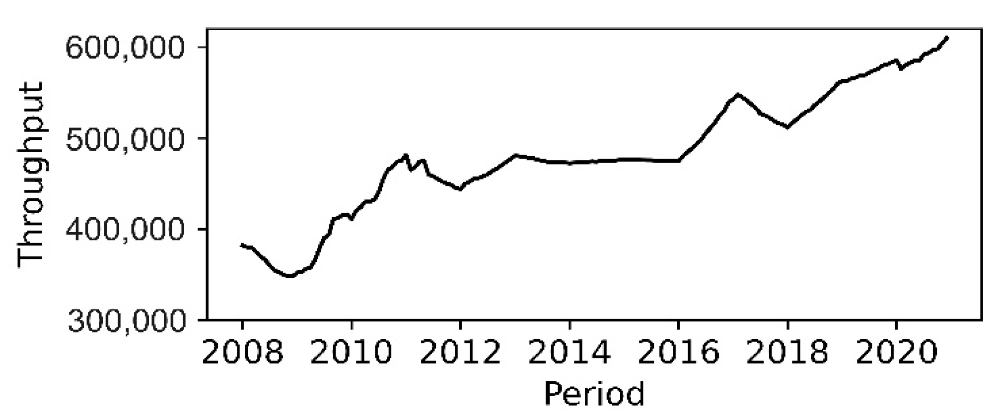UNCTAD [5] classified aspects of the cargo dwell time of the ports as an indicator of port performance, defined as the time between container discharge and exit from the port, which exceeds 21 days on average compared to less than a week in European ports. The Douala port system is not keeping up with the rising cargo volume and international trade or other technological practices that facilitate trade due to the port’s shallow water depth of about 11 m, its location towards a tight city center, and other port operations inefficiencies that hinder growth projects [6].

UNCTAD recently updated its port performance scorecard that was first drafted in 2012 as part of its port training program to benchmark port performance indicators (PPIs) and assist port managers with best practices in port assessments [5]. Amongst these indicators, berth and cargo operations had the most substantial mean influence on port performance between 2015 and 2019, showing their importance as PPI benchmarks. Forecasting container throughput (CT) from these key PPIs will help the port make informed port planning decisions to treat port performance bottlenecks with the urgency it deserves. Port performance’s definition, therefore, entails a sequence of moves related to vessel stay at berth, the pace of loading/unloading freight, and the nature of storage and inland transport efficiency in and out of the port area.

The remainder of the article has the following structure: a succinct literature review is explored in Section 2. Section 3 presents the materials and methods of the study. Section 4 describes the empirical study, while the results, analysis, and stochastic processes are deduced in Section 5. Finally, discussions, conclusions, and future directions are outlined in Section 6.

2. Literature Review

Since the initiation of container throughput forecasting in the 1980s, numerous studies have continuously proposed methods and model adjustments to achieve accuracy in container throughput forecasting. These methods can be divided into benchmark models, nonlinear modeling methods, and hybrid forecasting models. First, benchmark methods: Sepulveda-Rojas et al. [7] applied an adjusted moving average for a model selection criterion in throughput forecasting, saving time spent on model testing. Rashed et al. [8] applied the ARIMA model for container throughput forecast in the port of Antwerp, resulting in ARIMAX as an output series that is more accurate for throughput forecasting. Wang and Phan [9] utilized the grey model (GM) to model cargo throughput in Kaohsiung port, where they used a modified residual of the GM (1, 1)—Fourier residual modification GM (1, 1)—to improve performance accuracy. Chen et al. [10] applied a Grey–Markov model for container throughput forecast in Fujian Province, which proved their proposed draft as an accurate throughput forecasting model. Schulze and Prinz [11] made a comparative study on SARIMA and Holt–Winters exponential smoothing to forecast container transshipment in Germany, where the SARIMA model outperformed Holt–Winters exponential smoothing in forecasting accuracy. Second, nonlinear modeling methods: Mark and Yang [12] applied approximate least squares support vector machines (ALSSVMs) to model Hong Kong container throughput, where the results verified the superiority of the proposed model over the standard support vector machine (SVM). Chen and Chen [13] utilized genetic programming (GP) for forecasting Taiwan’s primary port throughput, where they verified the accuracy of the proposed method in throughput forecasting. Third, Hybrid models: Xie et al. [14] applied a hybrid least square support vector machine model (LSSVM) for container throughput forecasting in Shanghai and Shenzhen ports, where the hybrid model proved to be better than single models, while the LSSVM proved to model non-linearities in port time series. Niu et al. [15] proposed a hybrid variational mode decomposition (VMD), autoregressive integrated moving average (ARIMA), hybridizing grey wolf optimization (HGWO), and support vector regression for container throughput forecasts. The built method outperformed the comparison models in prediction accuracy. Xiao et al. [16] proposed a hybrid model based on improved optical swarm optimization and feed-forward neural networks (IPSO-FNNs) to model non-stationary time series in port throughput forecasting.

Although these studies were valuable in their respective methods, they were primarily based on univariate data structures. They forecasted throughput based solely on throughput’s lag observations, which might not be enough for an accurate forecast that provides insights required to improve critical port performance indicators (PPIs). As the financial crisis has made port time series volatile and nonlinear, benchmark methods fail to model this non-linearity due to their built-in linear assumptions on time series [14]. Simultaneously, the solid pre-assumptions and time series component adjustments made by benchmark models limit their ability to model nonlinear interactions with crisp accuracy. Additionally, there is limited research in the literature for port throughput forecasts based on multivariate data structures. Few studies, such as [17,18], forecasted port throughput from a multivariate predictor variable consisting of GDP, import/export and GDP, output value, and net export, respectively. Gosasang et al. [17] verified the performance accuracy of the MLP model over regression models in throughput forecasting, while [18] applied a genetic algorithm and backpropagation neural network (GA-BPNN) on Guangdong Province port throughput; the results show that their proposed model outperforms traditional methods in throughput forecasting. Additionally, [19] modeled port throughput from socio-economic factors through a novel multivariate adaptive regression adaptive spline and a robust v-support vector regression model (MARS-RSVR). Tang et al. [20] applied the socio-economic growth projection factors for container throughput forecasting in the port of Shanghai and Lianyungang.

Evidence from the prior literature proves that the focus of container throughput forecasting based on multivariate data structures was on socio-economic and growth projection factors such as supporting industry output, economic status of the nation, import and export, GDP, interest rate, and growth projection factors. Tally [21] noted that in evaluating the performance of a port, its actual and optimum throughput is compared, where an increase in throughput towards the optimum over time is considered an improvement in port performance and contrarywise. Thus, port performance can also be defined as a function of throughput. Tally [22] divided a port’s optimum throughput into engineering and economic throughput, whereby the former constitutes the actual throughput that a port can physically accommodate under certain constraints (port KPIs), while the latter represents the optimum throughput a port can handle based on socio-economic factors. A port needs to find leverage to identify and prioritize measures to improve its KPIs to attain growth opportunities, competitive advantage and become attractive to cargo providers (shippers and shipping lines). Recent studies focusing on cargo port choice determinants from shipping lines’ and shippers’ perspectives shed a brighter light on factors affecting a port’s performance (as a function of throughput). Omoke and Onwuegbuchunam [23], in the case of West African ports, deduced factors such as berth productivity, storage capacity, gate wait time, and ship turnaround time as critical for port performance, while in a global perspective, [24] deduced factors: terminal charges, terminal service quality, intermodal transport availability, nautical accessibility, hinterland connection, port reputation, and terminal operations. Even more studies [25,26,27] focused on defining the determinants of a port’s performance (as a function of throughput) for achieving port attractiveness and competitiveness in the perspective of cargo port providers (shippers and shipping lines) also proposed similar factors related to port operations. Besides, evidence from a recent port performance scorecard overview UNCTAD [3], depicting key benchmark port performance indicators (human resources, gender, vessel operations, cargo operations, environment, finance, and economic), proves that berth and cargo operations had the most significant mean influence on port performance (as a function of throughput) from 2015–2019. Therefore, it is crucial to model port throughput from a new angle—port operations factors. This paper is the first to appear in the literature to explore port operations factors for container throughput modeling. It will provide insights to assist port management in spooning out port bottlenecks, improving efficiency, attaining competitive advantage, and port attractiveness for cargo port choice criteria (shippers and carriers). This study will also provide a steppingstone for further research in the field of port performance and container throughput forecasting.

The focus of this study is summarized in three points. First, to forecast the engineering optimal throughput of Douala port from multivariate predictor variables associated with port operations through RF and MLP. Second, to provide an interpretation of the stochastic process and complex interactions between the predictor and response variables through feature importance by permutation and partial dependency plots. Third, to provide a hypothesis testing through four model evaluation criteria and seven competing models based on univariate and multivariate data structures. Results indicate that RF is a potential candidate for forecasting the engineering optimal throughput of Douala port, which can reduce uncertainty and provide leverage for port managers and stakeholders to spot and improve weak key performance indicators.

3. Materials and Methods

Our models’ framework—RF, MLP and a developed hybrid RF-MLP—is described briefly in the sub-sections that follow: Section 3.1 describes Random Forest, Section 3.2 describes multilayer perceptron, and Section 3.3 describes the developed hybrid model based on random forest and multilayer perceptron.

3.1. Random Forest

Random forest is a supervised ML algorithm that uses an ensemble method for regression and classification tasks. An ensemble is a method by which the RF model obtains an accurate prediction by averaging many independent weak decision tree predictions. The accuracy of an ensemble over individual members depends mainly on two necessary conditions. The individual tree members’ accuracy must be better than random guessing, and their errors made on unseen data must be uncorrelated or diverse [28].

The principle of RF is to consolidate a multitude of de-correlated trees on a separate set of observations [29], each of which is constructed using a bootstrap sample withdrawn from the original sample feature and a subset of parts and the average of the predictions of trees in the forest becomes the output of the model. This process is termed bootstrap aggregating or bagging. The main point in bootstrap aggregating is to reduce the variance by averaging the different approximately unbiased models in the forest. Some ensemble benefits, such as decreasing correlation through randomization, are exploited during bagging. The bias of the bagged trees always remains the same as that of the individual trees. Breiman and Cutler [30] explained that reducing the correlation between trees dramatically reduces the variance, and overfitting is minimized as more trees are added. Overfitting is shared equally amongst the trees in the forest, thus limiting the generalized error. Perhaps a valuable characteristic of random forests is the out-of-bag (OOB) sample: $L_{OOB,k}$. During bagging, to generate a train set for the ensemble members, observations are set aside and not used for training in the ensemble. This set is the out-of-bag sample. The generalization error is computed from this OOB sample. Random forests regressions’ measure of the goodness-of-fit is the R2 value, calculated from the random forests’ OOB mean squared error $mse$, and the dependable variable variance $var\left(y\right)$, as shown in Equation (1) [28].

$$R^2=1-\frac{mse(\left\{T_{L_{OOB}\left({\theta }_k\right)}\right\}{}_1{}^K)}{var\left(y\right)}$$

(1)

$$f\left(x\right)=\frac{1}{K}{\displaystyle \sum }_{k=1}^K{T}_{L\left(0_k\right)}\left(x\right)$$

(2)

For the learning process of random forest.

For $k=1$ to $K:$ (size of the ensemble). Extract a bootstrap sample data $L$ of size $N$ from the training data sample. Grow a tree $T_L,$ draw another bootstrapped sample $L\left(0\right)$ by iteratively repeating the following steps for each node until a minimum node size $n_{min}$ is reached.

• Select $H$ variables at random from the $m$ variables.
• Pick the best variable/split-point in the $H$.
• Split the node into two baby nodes.

Output the total of trees $\{T_L$}$q=1, 2, \dots .,k$. To predict a new point $x$, see Equation (2). The essential parameters here are the number of trees in forest K, and the number of randomly chosen variables at each split H. Experimenting is the recommended method in determining the number of trees for the model. The RF algorithm models such that, given an input $x_i={[x_{i,1} x_{i,2}\dots x_{i,n}]}^T$ and a labeled output $y_i={[y_i]}^T$ the algorithm (RF) tries to learn and approximate its underlying mapping function, such that with new data $x_i={[x_{i,1} x_{i,2}\dots x_{i,n}]}^T,$ it can predict the target output $y_i={[y_i]}^T$ based on what it learned from the data it was fed. For nonlinear models, higher-order variable interactions are taken into consideration, and as such, one cannot make assumptions that an increase in one variable will adeptly lead to an increase in the response variable in the same direction. The multifaceted nature of variable interactions in nonlinear models adds complexities to their interpretation. The partition of individual trees in the forest to extend an ensemble means that each sub-tree has a local prediction value independent of its tree neighbors. Averaging the ensemble to obtain the forest prediction locks the algorithm in a black box along with interpretability.

Therefore, the RF model stems from producing accuracy and practical implementation at the expense of interpretability. In a dynamic sense, one way to open the black box of random forest predictions to close the gap in interpretability with traditional models is by computing how independent features lead to a specific prediction, as every prediction can be presented as the sum of feature contributions. This is performed through feature importance by permutation, whereby the values of single variables of interest are shuffled, and a change in model accuracy is computed. A variable is important if shuffling its values decreases the model’s accuracy. For the variable importance measure based on permutation, $w_j\left(T_L\right)$ according to [28] is shown in Equation (3), where $L^j{}_{OOB}\left(0\right)$ is the OOB sample while the $j$ variable is permuted. The average of these important measures in individual trees to ensembles of trees is shown in Equation (4).

$$w_j\left(T_L\right)=mse(T_{L\left(0\right)})-mse(T_{L^j{}_{OOB}\left(0\right)})$$

(3)

$$w_j=\frac{1}{K}{\displaystyle \sum }_{k=1}^K{w}_j\left(T_{L\left(0_k\right) }\right)$$

(4)

A significance threshold (zero) is defined once variable importance measures are obtained to determine the significance of variables describing the response [28]. One approach is to exclude unimportant variables below the threshold. However, this method is said to be computationally costly as it necessitates the creation of several forests to obtain a distribution of the important measures.

The interactions of predictor variables in a multivariate structure add complexities to the model interpretation of influence. Interpreting the dependence of the response variable on independent predictor variables is considered to understand the stochastic process inherent in variable contributions to the outcome. Breiman and Cutler [30] suggested the partial dependence plots (PDPs) as a method of exploring what influence a variable of interest exerts on a response in any predictive model. Consider a dataset which includes $N$ observations $x$, of a response variable $y$, for $x=1,2,\dots , N$, along with $p$ covariate samples denoted $x_{ic}$ for $i=1,2,\dots , p$ and $c=1,2,\dots , N$. The predictor model, $f\left(x\right)$, is generated in the form shown in Equation (5).

$$f\left(x\right)=f\left(x_{1,c}, x_{2,c}, \dots x_p{,}_c\right)$$

(5)

For a single covariate $x_s$, and all other covariates $x_c,$ not included in $x_s$, the predictor model above can be summarized as $f\left(x_s,x_c\right)$.

Friedman’s partial dependence plots, in the case of a single variable of interest $x_s,$ is obtained over a range of $x$ values, where $x_{ic}$ are values of covariates in $x_c$, as shown in Equation (6).

$$f\left(x_s\right)=\frac{1}{N}\sum _{i=1}^{N}f\left(x_s,x_{ic}\right)$$

(6)

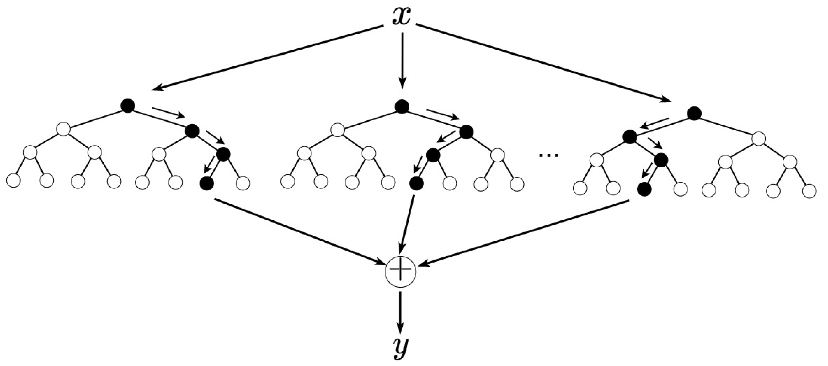
The partial dependence plot’s ability to investigate the nonlinear influence of predictor variables on the response is directly related to the model’s ability to approximate the input data’s underlying mapping. A schematic of an RF model is shown in Figure 1, depicting data movement by bagging through independent trees in the forest.

3.2. Multilayer Perceptron

MLP is a kind of artificial neural network developed through recursive functions and logical assumptions by an experimental study of neurons’ interconnections in a physical system. Thus, it replicates the human brain’s neural network structure. MLP is used for both regression and classification tasks and usually consists of artificial neurons, which transmit signals between each other. When a neuron receives a signal, it processes it and signals downstream neurons connected to it. Neurons are organized into layers called the input layer, hidden layer, and output layer. Neural networks have been applied to problems ranging from gene prediction and the classification of cancers to speech recognition. The adeptness of neural networks is that they can be used as a prediction/assessment or analytical model in solving just about any problem. One benefit of MLP applications is that they may be more accurate when modeling from complicated natural systems with a large sample size. The more complex the system (large sample size), the more accurate the model becomes. Examples of its application include but are not limited to: Kourounioti et al. [17] in predicting the dwell time of import containers in the port, [17] compared the autoregressive integrated moving average (ARIMA) model with the artificial neural network (ANN) model for container throughput forecasting which resulted in the ANN outperforming the ARIMA in forecasting accuracy.

The mechanism of the feed-forward network is that each neuron receives a noted input $x_i=\left[x_{i,1} x_{i,2}\dots x_{i,n}\right]$ and then random weights are initialized, denoted with $w_{ij}$. The inputs are then multiplied with the weights plus the bias $b_i$, an activation function is added to propagate the output of the first layer to the next layer in the network, as shown in Equations (7) and (8), where $w_{ij}$ is the weight of each node, $x_i$ is the input variable and $b_i$, the bias of each node (neuron), f is the activation function applied to every neuron, $n$ is the number of inputs from the incoming layer, and $i$ is the counter from 1 to $n$. Every layer in the model is represented as in Equation (8). The weights connect the neurons in the layers while the bias—a constant donated as 1, ensures the inputs propagates to the next layer. The activation function—ReLu, as shown in Equation (9)—is applied to every node.

$$u_i=\sum _{i=1}^n{w}_{ij}{x}_i+b_i$$

(7)

$$\mathcal{O}=f\left(u_i\right)$$

(8)

$$f\left(x\right)=max\left(0|x\right)$$

(9)

The rectified linear function (ReLu) works to transform an input ($x$) to the maximum of (0) or the input itself ($x$). Since a neuron cannot propagate to the preceding neuron with an output of zero, the bias $(b_i)$ ensures it fires forward by adding a value to it, denoted as 1. The output: $\mathcal{O}=f\left(u_i\right)$ is used as input in downstream nodes, while the process repeats iteratively depending on the number of hidden layers. After an epoch (a complete forward propagation from input to output layer), we compute the error by obtaining the difference of the residuals. The weights update is performed through backpropagation if the error is still large. The Adam solver is used as an optimization algorithm for the model. The objective of Adam is to minimize a given loss function as close to $zero$ as possible. The error function (difference of the residuals) is defined as shown in Equation (10).

$$l=\frac{1}{2} \sum _{i=0}^n{[{\gamma }_i-{\widehat{\gamma }}_i]}^2$$

(10)

where ${\gamma }_i$ is the observed value and ${\widehat{\gamma }}_i$ is the predicted value of the training set instance $i$. Weight optimization is performed by applying the chain rule of differential calculus. Weights are updated going backward from the output, hence the term backpropagation. The first weight from the output layer is updated by finding the derivative of the loss function in respect to the model output multiplied by the model output in respect to the weight. This is formulated as shown in Equation (11), while the weights in the second layer going backward are updated as shown in Equation (12). Each weight $w_i$ is then iteratively updated as shown in Equation (13).

$$\frac{\partial l}{\partial w_1}=\frac{\partial l}{\partial \theta } , \frac{\partial \theta }{\partial w_1} ,\frac{\partial \theta }{\partial w_2}, \dots ,\frac{\partial \theta }{\partial w_j}$$

(11)

$$\frac{\partial l}{\partial w_1^2}=\frac{\partial l}{\partial \theta } , \frac{\partial \theta }{\partial {\theta }_1} , \frac{\partial {\theta }_1}{\partial w_1^2} , \frac{\partial {\theta }_1}{\partial w_2^2}, \dots ,\frac{\partial {\theta }_1}{\partial w_j^2}$$

(12)

$$w_i={\widehat{w}}_{ij}-\eta \frac{\partial l}{{\widehat{w}}_{ij}}$$

(13)

By updating backward, $\theta$ is the output, $w_1$ to $w_j$ are the weights on the first hidden layer, ${\theta }_1$ is the output of the first hidden layer, $w_1^2$ to $w_j^2$ are the weights in the second hidden layer, and $w_i$ is a new weight, ${\widehat{w}}_{ij}$. The old weight and the constant $\eta$ is the learning rate which decides the length of steps towards a minimum for each iteration. While updating weights by backpropagation, the propagated error is also considered. Therefore, for each hidden layer, the backpropagated error values are computed as shown in Equations (14) and (15).

$${\omega }_r={\theta }_r\left(1-{\theta }_r\right) \sum _{C=1}^C{w}_{rc}{\omega }_c$$

(14)

$$\frac{\partial l}{\partial w_{pr}}={\omega }_r {\theta }_p$$

(15)

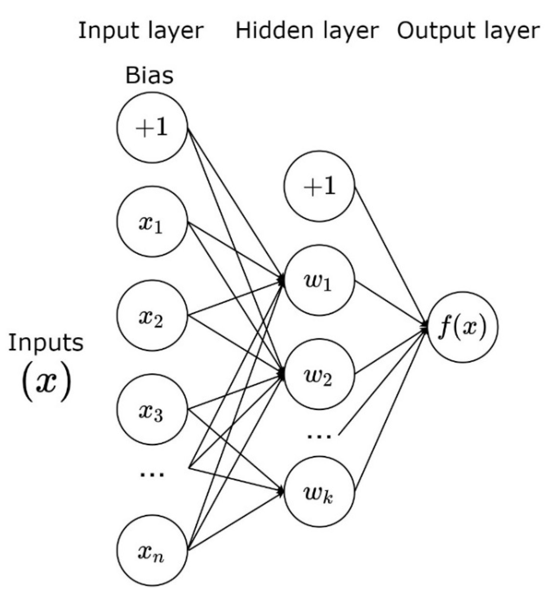
Here, $w_c$ is the weight from the successive nodes, $w_{rc}$ is the weights connecting the current node $r$, and successive node $c,$ and ${\theta }_r$ is the output of the current node. Thus, the backpropagated error ${\omega }_r$, and ${\theta }_p$ is the input value of the predecessor node, $p$. Figure 2 shows a schematic of a multilayer perceptron with input features, $\mathrm{x}=$ $\left({\mathrm{x}}_{1,} {\mathrm{x}}_2\dots {\mathrm{x}}_n\right)$, bias $\left(+1\right)$, weights $\left({\mathrm{w}}_1, {\mathrm{w}}_2\dots {\mathrm{w}}_k\right)$ and output $f\left(x\right)$—where $f$ is the activation function applied in every node.

3.3. RF—MLP

Both RF and MLP models have been used in prior research to model linear and nonlinear interactions with success. However, both models still have inherent drawbacks and are not suitable for all situations. 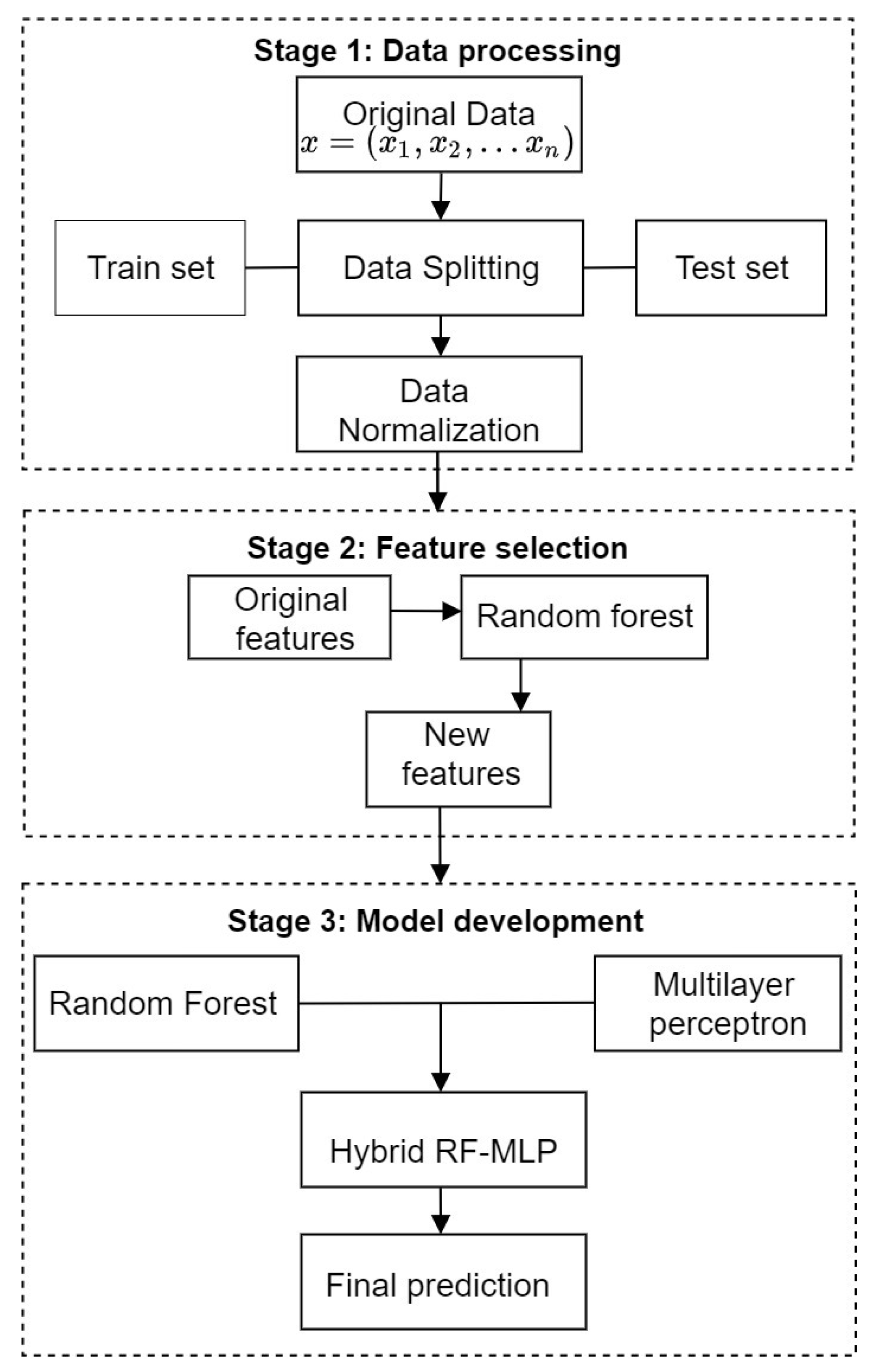For example, despite RF strengths in general resistance to overfitting, handling missing data, computing variable importance measures, and partial dependencies to describe variable interactions [30], the RF algorithm might change considerably with a slight change in the data, making them easy to overfit. On the other hand, MLP performance in throughput modeling depends mainly on the data’s size and noise level. Thus, aggregating both models’ strengths could lead to the capture of differential underlying patterns that could improve performance accuracy. A schematic of the coupling of hybrid RF-MLP is shown in Figure 3.

In stage one, we carried out data processing, where the original data were split into two subsets: the train set (80%), and test set (20%). The split data were then normalized to obtain a mean closer to zero for achieving faster convergence (speed up learning), and to ensure the min and max disparity in the input features were regarded to a similar extent by the model. The formula for normalization is shown in Equation (17) below.

$$x_i=\frac{X_i-min\left(X\right)}{\max \left(X\right)-min\left(X\right)}$$

(16)

where $x_i$ is the normalized value for $X_i,$X is the training set, while max(X) and min(X) determine the maximum and minimum values of the training set.

In stage two, we explored feature selection. First, the original features were trained with the random forest model (RF), then new features were created through a significance threshold determination criterion that quantifies the importance of the original features in function estimation. The feature importance measures were obtained by permuting the values of the original features, one at a time (see Section 3.1). Once feature importance measures were generated, a significance threshold (which was set to 0.0 for this study) determined the new features by eliminating truly unimportant variables below the threshold value. The new features imply a significant association between predictor and response. The mathematical theory of the RF model and feature permutation importance is described in Section 3.1.

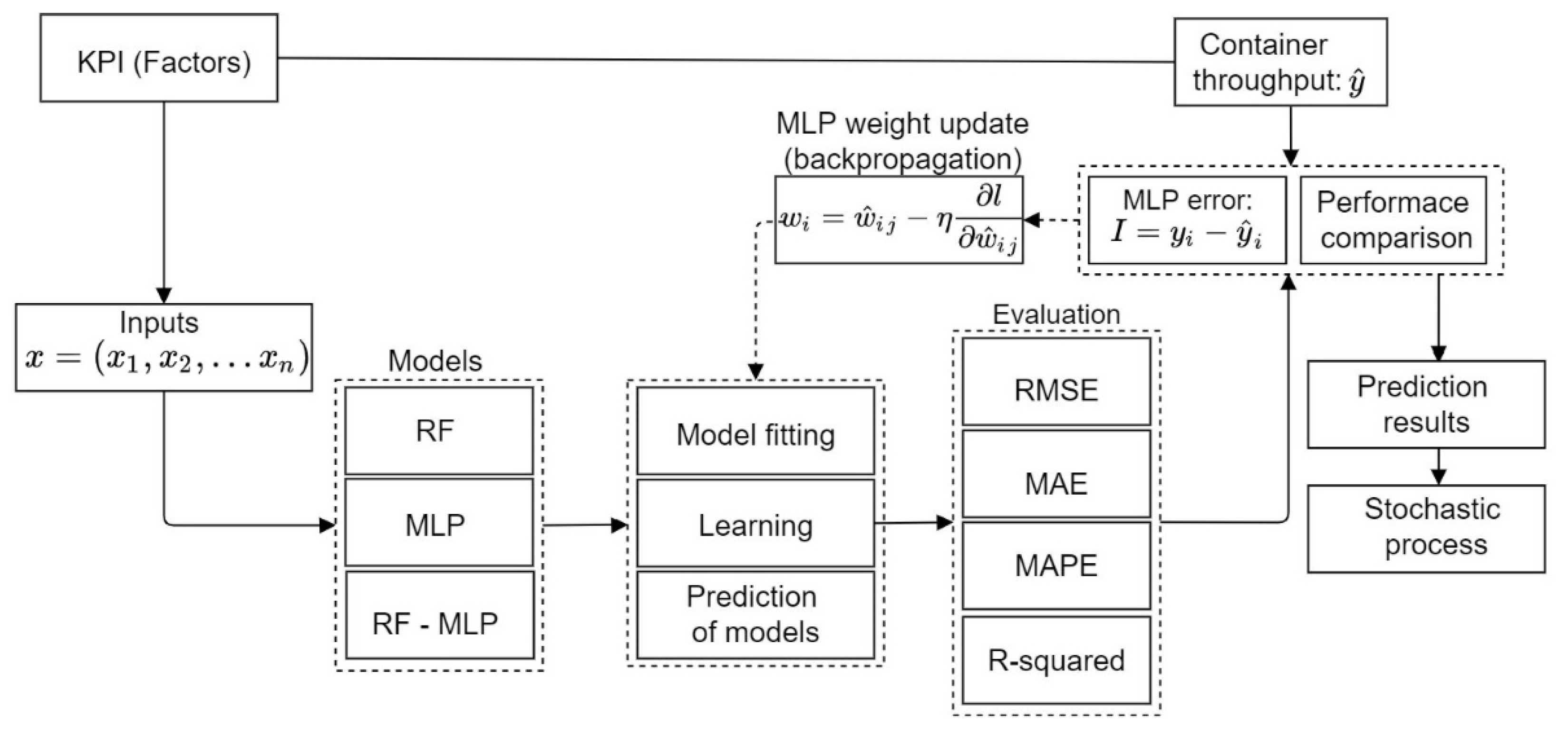
At the third stage, the hybrid model was developed based on random forest (RF), and multilayer perceptron. The new features, depicting significant association with the response, $x_i=\left(x_1,x_2,x_3\dots x_k\right)$, were used to construct training patterns for RF-MLP. The train set of the new features was used to fit the model to study the underlying mapping with known inputs and outputs, then the performance from the train set fit was estimated on new data (test set or holdout data) with unknown target values. The resulting test set error was then assessed through four error metrics: r squared, NRMSE, MAE, and MAPE. A schematic of the entire study is shown in Figure 4, below.

4. Empirical Study

4.1. Data Description

The port of Douala, Cameroon is located on the west coast of Central–West Africa and has a moderate drought of 11 m. It is considered a hub port for Central Africa as it serves neighboring landlocked countries such as the Central African Republic, Chad, and Northern Congo [4]. Douala port controls about 90% of total seaborne traffic into and out of the country. In 2019, container throughput (CT) at Douala port reached 7,310,000 million tons (growth rate of 0.05%), with an average growth rate of 0.04%. The study’s data are a multivariate time series of the operations dimension of the port’s KPIs, made up of six predictor variables in total. The data were obtained from the CEIC database (http://www.ceicdata.com/ (accessed on 29 June 2021)), a working paper on port performance scorecard [5], and ASYCUDA (automated systems for port custom data) provided by Cameroon customs. The data are a monthly time series covering the period 2008 to 2020, with 156 observations. The forecasting model in this study is constructed such that forecasts of any predictor variable $x_i=\left[x_{i,1} x_{i,2}\dots x_{i,n}\right]$ are not generated, but a single variable of type $y_i$(CT) is modeled as dependent on $x_i$, thus an open-loop system (CT depends on predictor variables STT, CTD, AVD, CSC, BP and ACDT for the forecasts and not vice versa). The monthly container throughput (CT) was designated as the response variable for this study, as shown in Figure 5.

The study variables were derived from berth and port cargo operations and include ship turnaround time (days), average vessel draft (meters), berth/crane productivity (container moves per hour), container dwell time (days), storage capacity (million tons), custom declaration time (days) and monthly container throughput (million tons).

The ship turnaround time (STT) is the gate wait time of a port measured in days. It is the time it takes a ship to gain access to the container berth, unload its tonnage, and leave. Most times, shipping lines are not affected by long gate wait times. However, if a nearby port adopts an optical character reader technology, leading to lesser gate wait times, then other shipping lines turn to notice an increase in gate wait times at the ports they serve. The second indicator—average vessel draft (AVD)—is the water depth of a port measured in meters and is considered one of the most important factors that determine a port’s attractiveness. The growth of containerization has been met with an emerging trend of mega vessels that demands intensive improvements in container terminals to match such size; thus, ports with a shallow water depth are set aside and serviced as spoke ports. Berth productivity (BP) can be defined as the average container moves per hour of crane activity on the berth. A port with inefficient gantry cranes could lead to congestion and time wasted for shipping lines and shippers. The average custom declaration time (ACTD) is measured in days; it is the time it takes for customs to clear goods after inspection within three hours of arrival at the port. In most cases, the declarant—the shipper responsible for the import—must ensure the goods are correctly valued, legitimate, and provide accurate information and authenticity of documents. Container dwell time (CDT), measured in days, is the amount of time cargo spends within a port upon arrival, which exceeds 21 days in Douala port. The shorter the dwell time, the lower the shipping line and terminal operating cost. Container storage capacity (CSC) is the measure of the container storage space in the port area (measured in million tons). The consequences of the above-mentioned port operations factors on the efficiency of the port of Douala depends mostly on their state and how accurately the port management employs its current resources to acquire an output (container throughput). In [31], port efficiency is defined as “relating to operational performance of a port and the employment of a limited resource in achieving an optimal output”. These factors are interrelated, and subsequently, inefficiencies in one element are likely to affect the other aspects. For example, inefficient terminal operations will feasibly constitute delays for hinterland operations. Below,

Table 1. Statistical description of the key performance indicators for Douala port.

Description	STT	CTD	AVD	CSC	BP	ACDT	CT
Count	156	156	156	156	156	156	156
Std	0.81	2.22	1.10	1.778	1.97	0.91	64.730
Mean	4.44	20.3	1.09	20.287	17.9	3.72	482.378
Min	3.10	14.0	8.50	15.000	11.0	2	347.779
Max	6.90	25.0	13.5	22.000	23.0	6	610.000

shows the statistical description of the variables included in the study.

4.2. Model Evaluation Criteria

For the evaluation of forecasting performance, since there is no unanimously proposed evaluation metric for use in every forecasting problem, several are typically used across forecasting models to provide a comprehensive evaluation. Based on [14,32], in this study, we consider four criteria frequently preferred to evaluate the forecasting performance of our pre-defined models. They are R squared, NRMSE, MAE and MAPE. With the absolute value present in both MAE and MAPE, they are both robust to outliers. The NRMSE, which is a non-dimensional form of the RMSE, facilitates comparison across models with different scales. The smaller the computed error through the other three evaluation measures (NRMSE, MAE, and MAPE), the better the accuracy of the model’s forecast. The error metrics are defined in Equations (16)–(19), respectively. Where $N$ is the number of sample size, $O_i$ and $P_i$ are the actual and predicted values, while $\hat{\mathrm{O}}$ and $Ƥ$ are the means of observed and predicted values, respectively.

$$R Squared=\frac{{\sum }_{i=1}^N(O_i-\hat{\mathrm{O}})\left(P_i-Ƥ\right)}{\sqrt{{\sum }_{i=1}^N{(O_{i }-\hat{\mathrm{O}})}^2{\sum }_{i-1}^N{(P_i-Ƥ)}^2}}$$

(17)

$$NRMSE=\sqrt{ \frac{1}{N}\sum _{i=1}^N|(O_i-P_i){|}^2 }$$

(18)

$$MAE=\frac{1}{N}\sum _{i=1}^N|\left(O_i-P_i\right)|$$

(19)

$$MAPE=\frac{1}{N}\sum _{i=1}^N\frac{O_i-P_i}{O_i}\times 100\%$$

(20)

Based on the requirement for performance assessment, apart from the MLP model, the RF and RF-MLP models were evaluated using a holdout dataset (train/test split) since the bootstrapping procedure of RF improves performance as it decreases the variance without increasing the bias by aggregating independent noise sensitive trees in the forest. The time series data were divided into a percentage of 80:20 for training and testing (holdout set), respectively. A total of 80% of the monthly throughput time series was used as a training dataset (124 observations from 2008 to 2017), and 20% (the remainder) was designated for evaluating the performance of the trained models. The training dataset was used to determine unknown parameters and train the pre-defined models to learn the time series underlying mapping. The testing dataset was used to evaluate the accuracy of the forecast performance from training. Data normalization was also performed to facilitate the model learning process (see Equation (16)). A five-fold cross validation was implemented to estimate the performance of the MLP model. The models were implemented in their basic form with the scikit-learn library in the python software foundation, version 3.8.5. After model evaluation, the model with the highest performance, the RF model, $f\left(x\right)=\frac{1}{K}\sum _{k=1}^K{T}_{L\left(0_k\right)}\left(x\right)$, was then used to model future indices. In addition, seven benchmark models were used in port throughput modeling, including multivariate decision trees (DT), least-squares support vector regression (LSSVR) based on kernel functions (nonlinear, polynomial and Gaussian). Support vector regression (SVR), autoregressive integrated moving average (ARIMA), seasonal autoregressive integrated moving average (SARIMA), linear regression (LR), and multiple linear regression (MLR) were applied for comparison with the proposed models in this study.

5. Results and Analysis

5.1. Proposed Model Results

The RF model achieves the best performance accuracy, followed by the hybrid RF-MLP model, while the MLP forecasting performance is lacking on all four measurement criteria (R squared, RMSE, MAE, and MAPE). Although the MLP model performed poorly as compared to RF and RF-MLP, it is still a good fit. The MLP model results are not surprising, as MLP mainly performs well with very large sample data to train on. A performance comparison for the proposed models (RF, MLP, and RF-MLP) with different measurement criteria—R2, RMSE, MAE, and MAPE—is shown in

Table 2. Prediction accuracy of RF, MLP, and RF-MLP.

Model	Test Data
	R Squared	NRMSE	MAE	MAPE
MLP	0.7565	0.2285	0.1786	2.9065
RF-MLP	0.9487	0.0667	0.0539	1.4441
RF	0.9878	0.0576	0.0375	0.9267

. The RF model with highest accuracy on all error evaluation criteria is depicted.

It is also crucial to examine the residuals which can add a comprehensive understanding to the goodness-of-fit. The residual is a measure of how well a line fits data points, and the closer the residuals of the data points are to 0, the better the fit and vice versa. Figure 6a–c, below, shows the residuals of the proposed models.

A comparison of predicted and observed values of performance accuracy on test data based on the model’s RF, RF–MLP, and MLP, respectively, is shown in Figure 7, below.

For comparison, the divergence of the forecasting potential between RF, RF-MLP, and MLP has been computed. From the forecast and observed values on the line plots, the RF model has the highest performance on predictions, while the hybrid model combining the random decision forest (RF) model and the artificial intelligence model (MLP) reveals slightly improved forecasting performance to the single MLP model. Thus, the RF model would provide more accurate capabilities for forecasting the optimal engineering container throughput (CT) of Douala port than RF-MLP, and MLP models.

Figure 8, below, shows the future forecast of container throughput (CT) of Douala port based on the RF model, while the future forecasted indices are described on

Table 3. Monthly future forecast indices of container throuput (CT) based on the RF model.

Month	Forecast
June 2021	581,503
July 2021	583,652
August 2021	585,244
September 2021	590,199
October 2021	592,718
November 2021	598,205
December 2021	606,108
January 2022	609,215

.

5.2. Comparisons

In contrast with all other models included for performance comparison in this study, benchmark models such as the ARIMA ($p,d,q$) and SARIMA ($p,d,q$) ($P,D,Q$) model is modeled following their inherent stochastic processes and assumptions. First, we extracted seasonal and trend components by decomposition, and checked for stationarity by the augmented Dickey–Fuller (ADF) test, which returned a null hypothesis with the assumption of non-stationarity. Then, we proceeded with differencing to correct the time series components and choose the order of our model by examining the autocorrelation function (ACF) and the partial autocorrelation function (PACF) plots from where our model is fitted. A comparison of seven popular methods in the container throughput modeling field with our proposed models is shown in

Table 4. Comparison of prediction accuracy with competing benchmark models.

Models		Test Data
		R-Squared	RMSE	MAE	MAPE
	Kernel *
LR		0.3592	0.3454	0.1812	6.1291
MLR		0.6057	0.1458	0.1203	4.4785
SVR	Linear	0.7300	0.1152	0.0968	2.3814
DT		0.7109	0.1336	0.0843	3.1431
MLP		0.7565	0.2285	0.1786	2.9065
LSSVR	Gaussian GBR	0.6895	0.1372	0.0993	3.8231
	Linear	0.7246	0.1323	0.0964	3.2433
	Polynomial	0.7720	0.1286	0.0926	2.4324
ARIMA		0.9249	0.0873	0.0754	1.5456
SARIMA		0.9308	0.0687	0.0404	1.3261
RF—MLP		0.9487	0.0667	0.0539	1.4441
RF		0.9878	0.0576	0.0375	0.9267

* The kernel functions map the original series from lower dimensional data into higher dimensional space in which they become separable and thus making the target function easy to predict (it captures the non-linear dynamics of the time series).

. SARIMA, RF—MLP, and RF are the models with the highest accuracy in ascending order.

For the ARIMA ($p,d,q$), SARIMA ($p,d,q$) ($P,D,Q$), linear regression (LR) and SVR methods, the multivariate nature of our predictor variables were ignored, and the models relied only on the lag observation of container throughput (CT). Nevertheless, the univariate nature of ARIMA and SARIMA did not limit their accuracy, as shown on the R2 accuracy score—0.9249 and 0.9308, respectively. However, their limitation lies in their inability to capture non-linearities and higher-order interactions in data, as they are considered typical linear models. Among all models included in this study, the LR model performed the poorest while including the multivariate predictor variables improved the MLR model’s performance. The polynomial kernel of the LSSVR based on a multivariate data structure had a better accuracy of 0.7720 than the SVR model, with a univariate data structure and R2 score of 0.7300. Based on the three initial models—RF, MLP, and RF-MLP for this study, the RF and RF-MLP models based on all measurement criteria—R2, RMSE, MAE, and MAPE—had the best performances relative to other models with an R2 performance accuracy of 0.9878 and 0.9487, respectively. The hybrid model, RF-MLP, performed just as expected in prior research [19], in which their study proposed novel hybrid models for container throughput modeling, and verified the performance accuracy of aggregating two models. The MLP did not perform as expected, given that the model’s accuracy in container throughput modeling had also been verified in prior research by [17], based on a multivariate predictor variable of GDP, import, and export. MLP’s low performance might be due to the different data distributions inherent in time series, the different variable interactions, and data structures (univariate and multivariate). The SARIMA model performed better than the ARIMA model because it described seasonality.

5.3. Further Analysis

From the results in Table 3, despite the RF high-performance accuracy on all evaluation measures—R2, RMSE, MAE, and MAPE compared to MLP and RF-MLP and all other models for comparison, the RF model is considered a black-box model, which favors accuracy over interpretability. Opening the black box of the RF model provides an understanding of the hidden complex nature and high-order interactions between the response and predictor variables. One approach is by permuting the predictor variables’ values and determining the decrease in model accuracy for each permuted variable (see Section 3.1 for a summary on permutation importance). A drop in the new model’s accuracy implies a significant association between the predictor and response. Figure 9 shows the significance of the variables by permutation.

The average vessel draft (AVD), a measure of the water depth of the ports’ terminal, has the highest contribution to the model’s prediction. The authors of [33] found that the vessel draft is one of the most crucial port infrastructure constraints for container terminals; as the mega vessel trend continues to grow, ports are obliged to employ infrastructural developments to meet up with the megatrends or risk being sidelined and served as spoke ports. The ship turnaround time (STT), container dwell time (CDT), and customs declaration time (ACDT), all have varying contributions to the model forecast. Container storage capacity (CSC) did not have any contribution whatsoever to the outcome of the model. This could be explained by the fact that the values of CSC were almost constant over the period of data collection because Douala port is located close to the city center, thus has limited expansion projects. As earlier mentioned in the description of the RF model, the CSC variable was dropped as it is notably useless to the model’s prediction. The important factors deduced by the prediction model indicate that port operations factors are essential for forecasting the optimal engineering throughput of Douala port.

While permutation feature importance does a great job at describing the level of association between multivariate predictor variable interactions with the response variable, the response variable’s dependence on a single predictor variable is reflected for further interpretability. Partial dependence plots (PDPs), which reflect a marginal dependence on a single predictor variable of interest for the model’s predictions (see Equations (5) and (6)), are shown in Figure 10, depicting the partial dependence of the response variable on four predictor variables of interest.

From the partial dependence plots, BP (berth productivity) increases almost proportionately with container throughput (CT) before stabilizing at 16 container moves per hour. On the second plot, an increase in gate wait times for ships or ship turnaround time (STT) to four days shows a stable decrease in container throughput (CT). Finally, for CDT (container dwell time), an increase in container dwell time sees container throughput (CT) decreases steadily. The PDPs structure shows an insightful distribution of the linear and nonlinear systems inherent amongst the variables.

However, it should be noted that PDPs investigating the dependence of the response on independent predictable variables of interest do not explain the entire model but rather the marginal influences of single variables and their value interactions. Thus, the idea of single directional influence is destroyed. The approach of permuted feature importance and partial dependence plots reveals the actual inherent structure of the system. Simultaneously, the dependence of the response on independent predictor variables is averaged to obtain better prediction accuracy.

6. Discussions and Conclusions

Port throughput forecasting is imperative in port management. It is a valuable and essential aid to planning, and planning is the foundation of efficient port operations. Amongst the very few studies in the container throughput modeling literature on multivariate time series, socio-economic, and growth projection factors, i.e., with factors such as GDP, interest rate, import/export, total output value, fixed asset investment, and population size had been employed to model the optimal economic throughput of a port. This paper is the first to appear in the literature to explore port KPIs associated with port operations for modeling the optimal engineering throughput of a port. This study offers insightful knowledge that assists a port in optimizing bottlenecks in port. Therefore, it is vital to achieve accuracy and interpretability in throughput forecasting. Additionally, while the importance of improving port KPIs is common knowledge in the logistics field, countries such as Cameroon and other developing nations fail to confront this issue with the urgency it deserves. Port KPIs have increasingly become central to every port’s performance, which is why it is crucial to understand which of these indicators affect or contribute to a port’s growth.

6.1. Implications

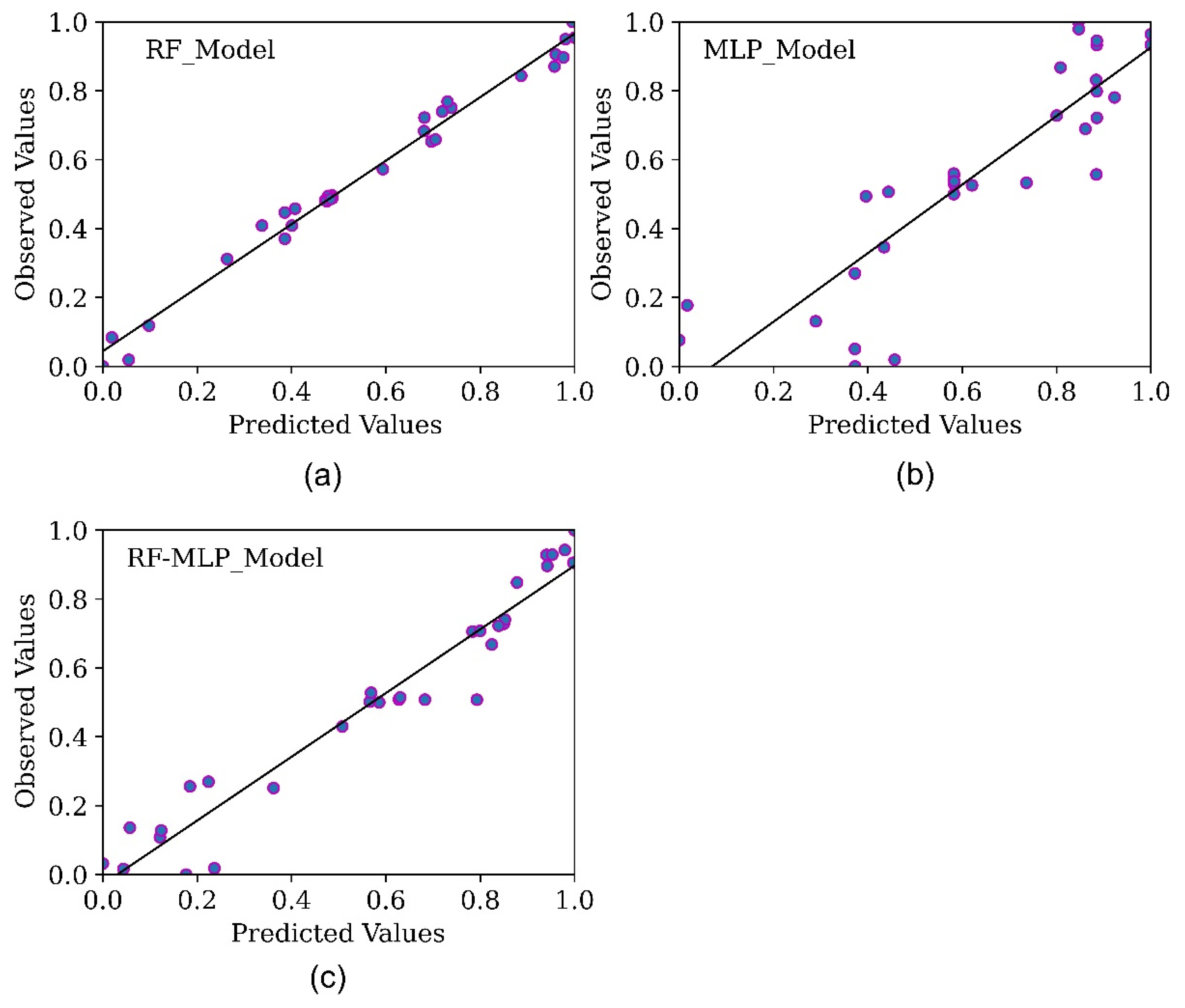
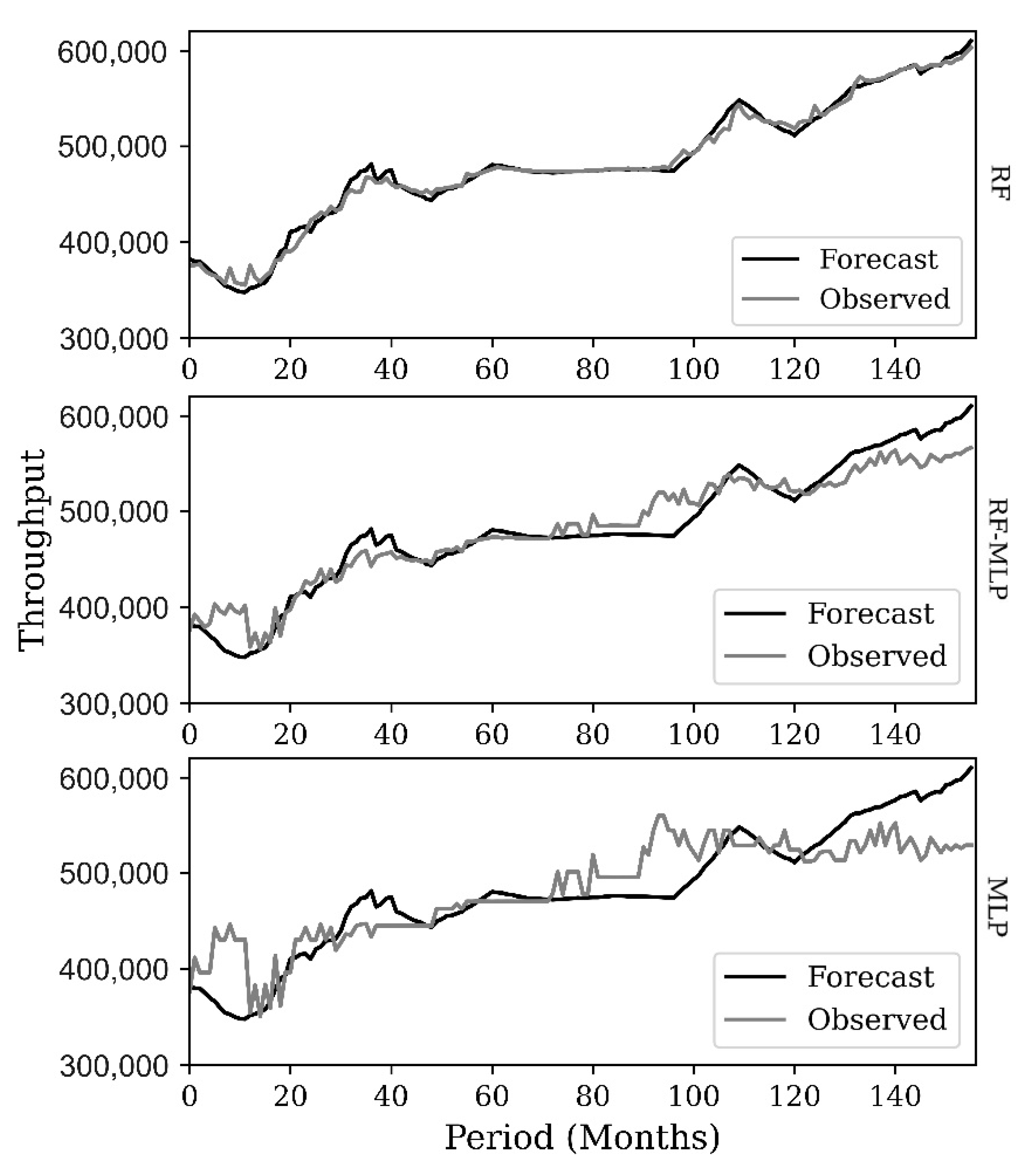
This study explored models—RF, MLP and RF-MLP—for port throughput forecasting and emphasized modeling from a multivariate process variable on KPIs associated with port operations. Performance comparison with other throughput modeling methods is also provided. All models, both proposed and comparison models, were applied in their basic form. The results imply that the RF model is effective with multivariate variables in forecasting the optimal engineering container throughput of Douala port for two reasons. First, it decreases the correlation between process variables through randomization by employing random split selection during bagging. Second, its complex nature lets it capture the complexities and higher-order variable interactions inherent in port time series, which is interpreted through feature importance and partial dependence plots. With its complex nature, the RF model is a potential candidate for forecasting the optimal engineering throughput of a port. The strength of the RF model is also inherent in the hybrid RF-MLP model results on the R2 value (goodness-of-fit)—0.9487, as aggregating their advantages enhances the prediction accuracy of the MLP model based on the R2 score from 0.7565 to 0.9487, respectively. Besides, its relatively small number of tunable parameters, automatic handling of missing data, generalization errors, and resistance to overfitting make it less complicated and easy for application. Based on the findings of this study, the proposed variables can be applied to similar studies to assist port management in improving their KPIs and overall efficiency.

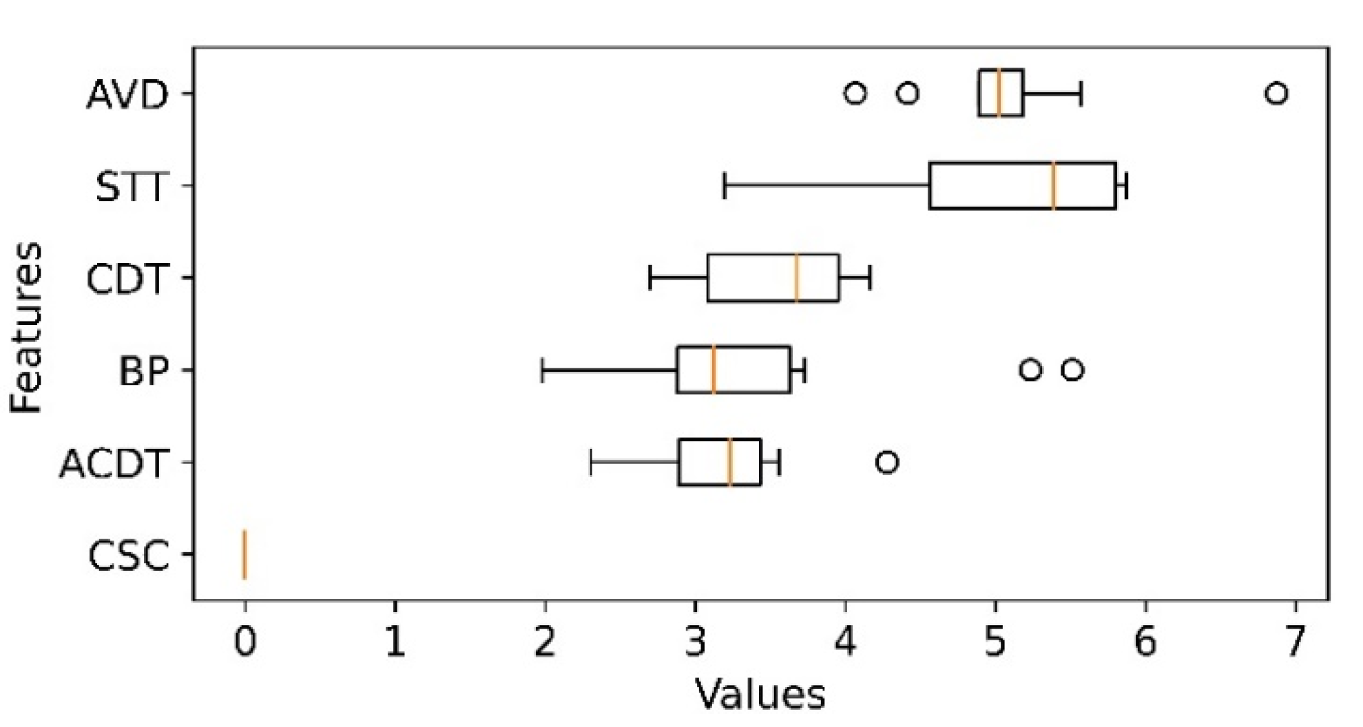
In today’s world, ‘uncertainty is opportunity.’ The forecasting task is a type of prediction that helps map out that uncertainty by exploring the underlying mapping of past and current data. This allows organizations to carry out an objective quality assessment—to consider the possibilities for better decision making with fewer risks. This study’s findings will provide significant insights to the port management of Douala in engaging in port planning and development projects in improving their port KPIs, which will potentially lead to improving port attractiveness and attaining international competitive objectives. 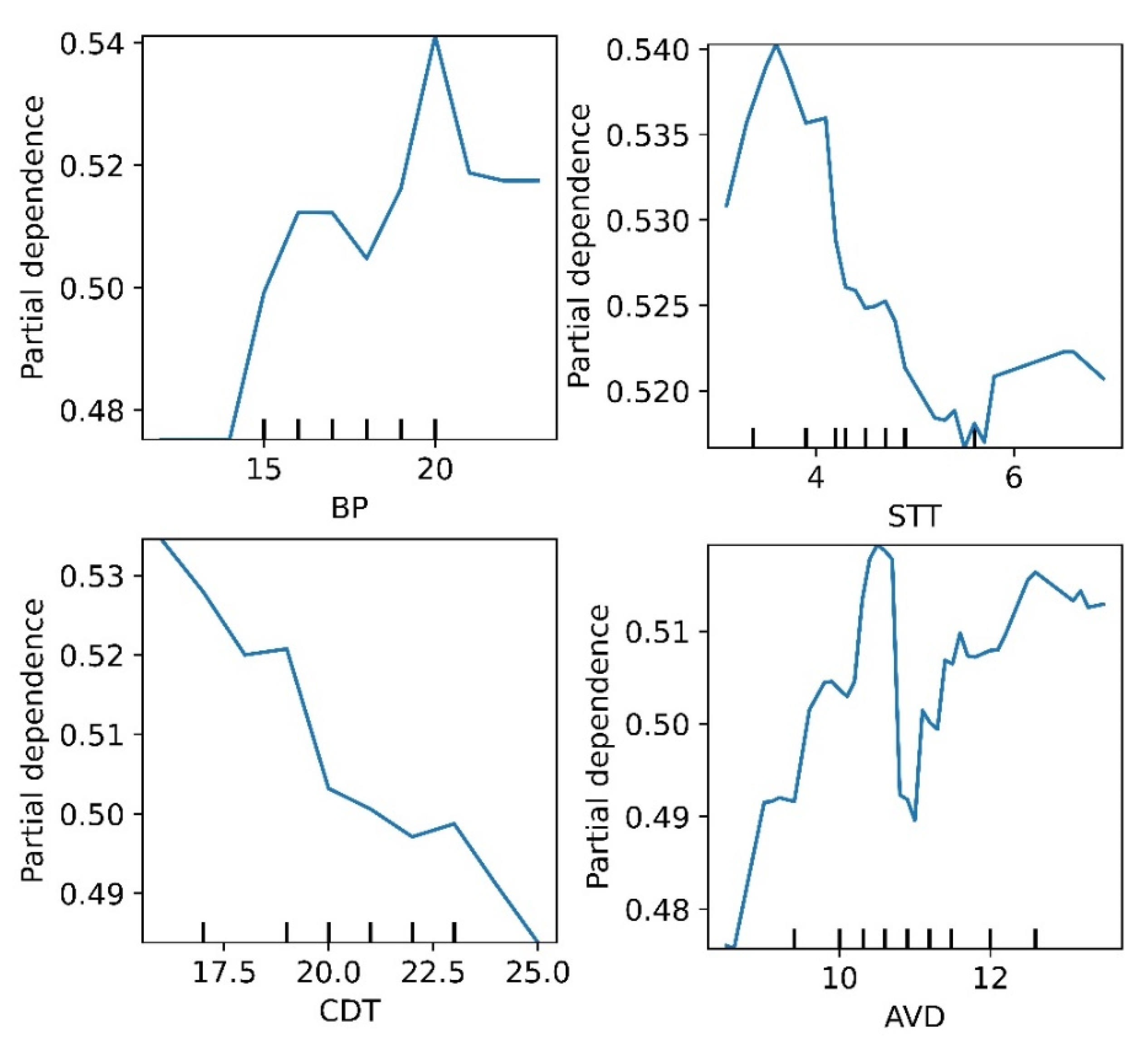Practically, from the obtained results, the RF feature permutation importance (see Figure 7) portrays the contribution of vessel draft (AVD), ship turnaround time (STT), container dwell time (CDT), and berth productivity (BP) in order of merit as the most important predictor variables for the models’ forecast. These variables should be the most vital to port management when engaging in port development projects. The PDPs on the four most important predictor variables of interest (AVD, STT, CDT and BP) further depicts how much improvement should be made on each predictor variable to attract more container throughput to the port. For instance, according to the PDPs (see Figure 8), AVD should be improved to 13 m through intensive dredging projects, berth/crane productivity to 20 container moves per hour by enforcing more terminal equipment, and CTD should be reduced to under 10 days by implementing new fiscal regime reforms, as [4] found that long cargo dwell times at Douala port are because of the fiscal pressure from port management. Finally, STT should be reduced to a minimum of 2 days by increasing the number of berths or length of container quay. Sheikholeslami et al. [34] found that increasing the length of quay reduces wait times of container ships by applying a simulation-based analysis.

6.2. Limitations and Suggestions

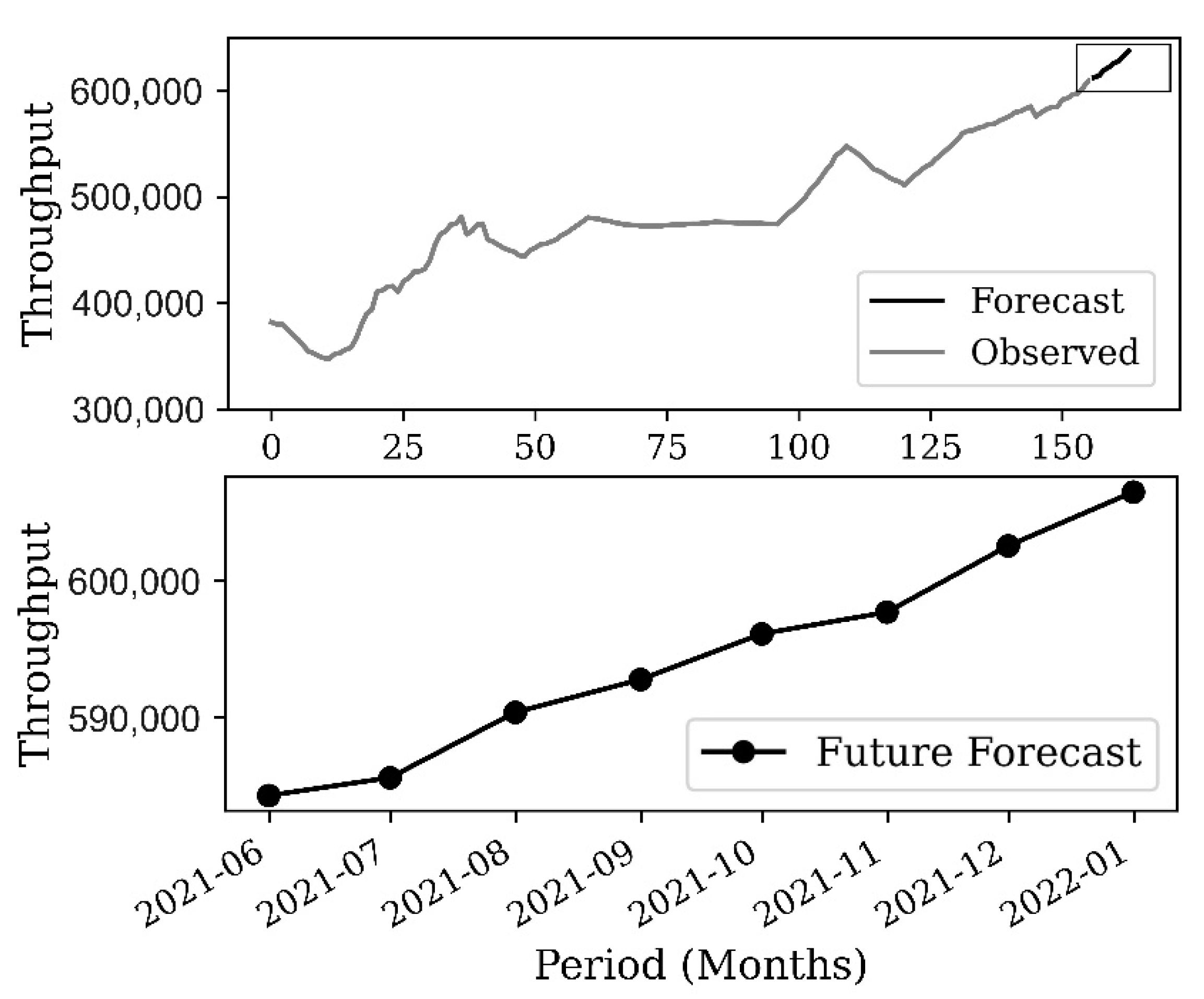
These results must be interpreted with caution, and a few limitations should be borne in mind. First, initially, we only considered a few factors due to data unavailability and we did not consider other competing benchmark models for comparison. Second, the ML models in this study were applied in their primary forms without modifications proposed in prior research; this is because the focus of the study was on a new variable application which should become a steppingstone for future studies. Third, the RF model applied in this study has a limitation to extrapolation, which is why we only considered a short-term throughput forecast. Due to the different data distributions and sample sizes inherent in container throughput time series, model applications across different datasets often give differential results. Therefore, for future directions, more port operations factors, external factors constituting regional center and hinterland connectivity index, and model modifications should be included and compared with even more competing benchmark models. For the different data distributions, to obtain a reliable forecasting result, trials should be focused on finding models that fit best given the data distribution or sample size.