Influence of Combined Motion of Pitch and Surge with Phase Difference on Aerodynamic Performance of Floating Offshore Wind Turbine

Abstract

Platform motions induced by waves pose a challenge to accurately predict the aerodynamic performance of floating offshore wind turbines (FOWTs). In view of this, the power performance and wake structure of FOWTs under platform pitch, surge, and their combined motions were investigated in this paper, using the computational fluid dynamics software, STAR-CCM+, with overset meshing and rigid body motion techniques. First, the simulation cases in single and same-phase combined motions with different amplitudes and frequencies were performed. Afterward, the approach of calculating the phase difference between pitch and surge motions was proposed to investigate the influence of the combined motion with phase difference on the aerodynamic performance. Results show that the increment of amplitude and frequency augments the mean power output and aggravates the power fluctuation in single and same-phase combined motions. The intensity of power variation under combined motion with a phase difference is weakened at 0.1 Hz compared to the single motion, while enhanced at 0.2 Hz, showing a different influence law on the aerodynamic performance. In addition, this paper established the power fluctuation table based on real sea states of Shidao in China, providing a certain reference for the controller design in this sea area.

1. Introduction

As onshore wind power has developed to a certain scale and is limited by space and utilization rate, the offshore wind power industry is gradually becoming an important development field. According to the Global Wind Energy Council 2021 report [1], the newly installed offshore wind power capacity in 2020 reaches 6.1 GW, accounting for 7% of the new installed capacity of global wind power, and the total installed capacity is up to 35.3 GW, representing 4.75% of the total wind power. Compared with fixed offshore wind power, floating offshore wind turbines (FOWTs) have the advantages of being free from water depth limitation, more convenient installation, operation, maintenance, and more abundant wind resources [2]. As a result, floating offshore wind power is becoming more and more popular among developers. The world’s first floating wind farm, Scotland’s Hywind, was built in October 2017, using a single-column floating installation with a total installed capacity of 30 MW [3]. The first wind turbine of the semi-submersible floating wind farm Windfloat Atlantic, with a total installed capacity of 25 MW, was connected to the electricity grid in January 2020 [4]. Research by the US National Renewable Energy Laboratory (NREL) showed that the cost of FOWTs is likely to fall faster than that of fixed offshore wind turbines. Although the FOWT is exposed to severe ocean conditions, the multiple degrees of freedom (DOFs) motions will have complex coupling effects on the aerodynamic performance of the wind turbine. The objective of this research is to study the unsteady aerodynamic performance of the FOWT under platform motions. Among six DOFs motions, surge and pitch DOFs seem to be the largest amplitudes modes for most platforms [5], leading them to be chosen for the investigation.

At present, a considerable number of scholars have focused on the aerodynamic performance of wind turbines, as shown in

Table 1. Publication related to the analysis of pitch and surge motion of the wind turbine.

Authors	Pitch (°)	Surge (m)	Frequency (Hz)	V 1 (m/s)	Method
De Vaal [8]		4, 8, 16	0.02, 0.04, 0.08	11.2	BEM
Tran [9]	0.01, 0.1, 0.5, 1, 4		1/30, 0.05, 0.1, 0.2	8, 11	UBEM
Wen [10]	1, 2, 3		0.05, 0.1, 0.2	11.4	FVM
Wen [11]		0.5, 1.5, 2.5	0.03, 0.1, 0.2	11.4	FVM
Farrugia [12]		0.916~4	0.065~0.2	6, 11.4, 18	FVM
Jeon [13]	3		0.083	4.5	VLM
Tran [14,15]	1, 4		0.1	11	CFD
Leble [16]	3, 5		0.1136	11	CFD
Lienard [17]	4, 8	8, 16	~0.1	11.4	CFD
Kyle [18]		9.4	0.1234	7, 11.4	CFD
Chen [19]	1, 4	1, 2	0.1, 0.2	11.4	CFD
Wu [20]	0.85		0.1	8, 11.2	CFD
Rockel [21,22]	16~19		1.2~1.8	6.05	Experiment
Fu [23]	5, 10, 20		0.6, 1.2	8.48	Experiment
Hu [24]	5		0.3	3.5	Experiment
Bayati [25]	1, 3	0.01, 0.1	0.65, 2.1	2.33, 3.67	Experiment

¹ Wind speed.

. Jonkman et al. [6,7] developed a modeling tool based on the blade element momentum theory (BEM) to simulate and analyze the dynamic behaviors of FOWTs. De Vaal [8] pointed out that the BEM method overestimates the aerodynamic damping, and there exist significant differences in the average induced velocity. Tran et al. [9] integrated the equivalent average velocity into the unsteady blade element momentum theory (UBEM). They found that the power and the thrust calculation results under small angle motion (1~2°) are similar to the CFD simulation results, but the discrepancy is as high as 24% under large-angle motion (4°). In a word, the traditional BEM method has some theoretical limitations and needs to be further optimized to calculate the complicated aerodynamic loads.

The free vortex method (FVM) based on the potential flow theory was first proposed by Sebastian [5,26,27]. It can accurately calculate the aerodynamic loads of wind turbines in motion and effectively capture the turbulent wake vortex as it can represent the actual physical flow field. Wen [10,11] adopted the FVM to study the influence of surge and pitch motion on the power and the axial thrust of the Spar type FOWT, and proposed the reduced frequency factor to integrate the influence of the amplitude and the frequency. The results revealed that when the reduced frequency increases, the average power decreases at the low tip speed ratio but increases at the high tip speed ratio. Farrugia [12] replicated the aerodynamic phenomenon observed in experiments based on the open-source free trailing vortex algorithm. It was concluded that the variation amplitude of the aerodynamic loads increases with the larger blade tip speed ratio, and a linear relationship between the surge velocity and the aerodynamic loads was also developed. In addition, Jeon [13] used a vortex lattice method (VLM) to predict the aerodynamic performance of FOWT, which was in good agreement with the experiment.

The FVM and the VLM can capture the unsteady aerodynamic phenomena to a certain extent; however, both are based on the ideal fluid assumption; therefore, many studies focus on computational fluid dynamics (CFD) with higher fidelity to gain the flow field information around the moving wind turbine. Tran et al. [14,15] investigated the influence of different pitch motions on the aerodynamic loads of the wind turbine based on the $k-\omega$ SST turbulence model. They indicated that the unsteady aerodynamic loads of the blades are significantly affected by the motion amplitude and frequency. Leble [16] studied the influence of pitch and yaw motion on the aerodynamic performance based on the DTU 10 MW wind turbine model. It was concluded that the pitch motion with a period of 8.8s and amplitude of 3° could not cause the wind turbine to enter the vortex ring state, while the wind turbine enters the vortex ring state at the pitch amplitude of 5°. Lienard [17] studied the aerodynamic performance of wind turbines under pitch and surge motion, respectively. The results suggest that the main reason for the load variation is the significant change of the attack angle rather than the relative local speed. Kyle [18] investigated the effect of surge motion on the wake state of the wind turbine and found that the blade root can more easily enter the vortex ring and propeller state as the attack angle at the root is smaller than that at the tip. Chen [19] compared the variation of global loads between combined motion and single motion. It was illustrated that the average power under the combined motion is smaller than that under the single pitch motion.

Moreover, many researchers apply experimental methods to study the influence of platform motion on wind turbines. Rockel [21,22] carried out an experiment of floating wind turbines under pitch motion at Portland State University and compared the experimental data with four wake model simulations. They noticed that the development area of the wake is nearly 0.7~7 D behind the wind turbine, and none of the four wake models can describe the wake development in detail. Hu [24] also conducted experiments of the wind turbine under the prescribed pitch motion through the high-resolution digital particle image velocimetry (PIV) system to measure the flow field information. It was concluded that the development of the wake under pitch motion is highly dependent on the direction, the amplitude, and the frequency of the platform motion.

Many scholars have researched the influence of platform motions on wind turbines, especially pitch and surge motions. Some scholars have also conducted simulations on the combined motion of the two, but without considering the phase difference between the two motions. The research results presented by Cheng [28] revealed that the platform surge motion has an opposite variation law compared to the pitch motion. Therefore, the aerodynamic characteristics under combined motions of pitch and surge with different frequencies, amplitudes, and phase differences were investigated in this paper. Furthermore, most scholars use ideal values of motion amplitude for the convenience of analysis. If the selected amplitudes were based on real motion conditions, the simulation results would have more practical engineering significance. Hence, the power variation table was constructed under the actual possible platform motions in Shidao in China.

2. CFD Simulation Model

2.1. Introduction of Turbine Parameters and Platform Motions

The selected NREL 5-MW wind turbine model is widely used in the FOWT simulation calculation. It is a traditional three-blade wind turbine, with a rotor radius of 63 m and a hub height of 90 m. The blades are comprised of DU and NACA airfoils from the hub to the tip. The rated wind speed is 11.4 m/s, and the rated rotational speed is 12.1 r/min. This research aimed to simulate and analyze the influence of platform motions on the aerodynamic performance of the wind turbine at the rated state (rated wind speed and rated rotational speed), considering the tower but without the controller. All related parameter information of the NREL 5-MW wind turbine can be found in Jonkman’s literature [29], and more information about the characteristics of the wind turbine can be found in

Table 2. Design parameters of the NREL 5-MW wind turbine.

Parameter	Value
Rated mechanical power	5.2966 MW
Rated electrical power	5 MW
Rotor orientation, configuration	Upwind, 3 blades
Rotor, hub diameter	126 m, 3 m
Hub height	90 m
Cut-in, rated, cut-out wind speed	3 m/s, 11.4 m/s, 25 m/s
Cut-in, rated rotation speed	6.9 rpm, 12.1 rpm
Rated blade tip speed	80 m/s
Shaft tilt, pre-cone	5°, 2.5°

.

Unlike fixed offshore wind turbines, FOWTs usually have a mooring system to limit the 6 DOFs motions of the floating platform within a certain range. The 6 DOFs motions include three translational components (surge, sway, and heave along the XYZ axis, respectively) and three rotational components (roll, pitch, and yaw around the XYZ axis, respectively), as shown in Figure 1. There usually exist coupling effects between motions and the external environment. Moreover, these effects will aggravate the aerodynamic unsteadiness of the wind turbine, such as blade tip vortex interaction, dynamic stall, wind shear, etc., posing more challenges to the design of the wind turbine. The traditional BEM method is not sufficient to capture these unsteady phenomena [30,31], so a high-fidelity simulation tool such as CFD is needed to study the aerodynamic characteristics of floating offshore wind turbines.

2.2. CFD Approach

The CFD computations were performed using the STAR-CCM+, which solves the unsteady Reynolds-averaged Navier–Stokes (RANS) equations. The implicit unsteady solver was selected in the STAR-CCM+, and the second-order central difference format was used for time discretization. Rigid body motion (RBM) and superimposed motion technology were used through user-defined field functions to define the combined motion. The overlapping grid technology was used for the grid data exchange between the wind turbine motion domain and the far-field background domain. For an incompressible, transient, viscous fluid, the RANS equations are generally solved based on the mass continuity equation and the momentum equation, which can be expressed as:

$$\nabla \cdot \mathit{U}=0$$

(1)

$$\frac{\partial \left(\rho \mathit{U}\right)}{\partial t}+\nabla \cdot \left(\rho \left(\mathit{U}-{\mathit{U}}_g\right)\mathit{U}\right)=-\nabla p_d-\mathit{g}\cdot \mathit{x}\nabla \rho +\nabla \cdot \left({\mu }_{eff}\nabla \mathit{U}\right)+\left(\nabla \mathit{U}\right)\cdot \nabla {\mu }_{eff}+{\mathit{f}}_{\mathit{\sigma }}$$

(2)

where $\mathit{U}$ denotes the velocity field of fluid, ${\mathit{U}}_{\mathit{g}}$ represents the velocity field of grids, $p_d=p-\rho \mathit{g}·\mathit{x}$ denotes the dynamic pressure, $\mathit{g}$ is the gravity acceleration, $\rho$ is the fluid density, ${\mu }_{eff}=\rho \left(\nu +{\nu }_t\right)$ is the effective dynamic viscosity, in which $\nu$ and ${\nu }_t$ are the kinematic viscosity and the eddy viscosity, respectively, ${\mathit{f}}_{\mathit{\sigma }}$ represents the source term that works at the free surface. To meet the closure requirement and solve RANS equations, the Menter’s shear stress transport (SST) $k-\omega$ turbulence model [32] was applied. It is a two-equation, eddy-viscosity turbulence model as follows:

$$\frac{\partial \left(\rho k\right)}{\partial t}+\nabla \cdot \left(\rho \mathit{U}k\right)=\nabla \cdot \left({\Gamma }_k\nabla k\right)+{\tilde{P}}_k-D_k+S_k$$

(3)

$$\frac{\partial \left(\rho \omega \right)}{\partial t}+\nabla \cdot \left(\rho \mathit{U}\omega \right)=\nabla \cdot \left({\Gamma }_{\omega }\nabla \omega \right)+{\tilde{P}}_{\omega }-D_{\omega }+Y_{\omega }{+\mathrm{S}}_k$$

(4)

where ${\Gamma }_k$ and ${\Gamma }_{\omega }$ are the effective diffusivity of the turbulent kinetic energy k and the specific dissipation rate $\omega$, respectively, ${\tilde{P}}_k$ and ${\tilde{P}}_{\omega }$ are the turbulence production terms, $D_k$ and $D_{\omega }$ are the turbulence dissipation terms, $Y_{\omega }$ is the cross-diffusion term introduced by blending the standard $k-\omega$and $k-\epsilon$ models. Wall functions were adopted automatically for near-wall treatment according to the near-wall grid size.

2.3. Simulation Setting

As seen from Figure 2a, the entire fluid domain contains three parts, including the background domain, the rotor domain, and the tower domain. The dimension of the background domain is 10 D × 6 D × 3 D (L × W × H), where D is the rotor diameter. The experiment results revealed that the wake of the wind turbine has a range of about 7D [22], so the inlet and the outlet boundaries of the background domain are 3D and 7D away from the wind turbine, respectively. The rotor domain is a cylinder with a diameter of 1.1D, a height of 16 m, and a centerline along the axis of the shaft.

In this work, the inlet, top, and side of the background domain were set as a velocity inlet with a magnitude of 11.4 m/s and a turbulence intensity of 1%. The outlet of the background domain was set as the far-field sea-level pressure outlet. The bottom of the background domain was set as the non-slip wall, as well as the turbine and tower surface.

Figure 2a also reveals the detailed grid of the background domain, the rotor domain, and the tower domain, with a total of 19 million grid cells. The mesh is the orthogonal grid generated by the AUTOGRID tool of STAR-CCM+ [33]. Figure 2b shows meshes of three regions that overlap with each other. Among them, the fluid domain has 9 million grid cells, which is enough to realize the transition from the inflow state to the internal fluid domain; the tower domain has 0.8 million grid cells; the rotor domain has 9.5 million grid cells. Fine mesh is generated on the blade surface as plotted in Figure 2c,d to ensure that the y+ value is between 10 and 100, which satisfies the requirement of the $k-\omega$SST turbulence model [20].

Table 3. The number of grid cells in the rotor domain.

Cells Number (Million)	1.8	3.0	5.6	7.2	9.5	12.5
Torque (106 N·m)	2.37	3.2	3.19	3.81	3.92	3.96
Relative error (%)	43.3	23.44	23.68	8.85	6.22	5.26

shows the calculated value of rotor torque with the different number of grid cells in the rotor domain. Taking the design torque value 4.18 e⁶ N·m under rated wind speed as the reference, 9.5 million was selected as the appropriate number for further simulation research due to the low relative error (6.22%) and moderate computation cost.

The steady-state computation was first completed after 1000 iterating steps, and its results were set as the initial condition of the unsteady-state simulation. Then, four cycles of unsteady-state simulations with a large time step and six cycles of unsteady-state simulations with a small-time step were performed. Finally, the simulation results of the last two cycles were taken as analysis data. The small-time step was set as the time for the rotor to rotate 2°, approximately 0.02775 s. All simulations were performed on a parallel computing workstation, which had a 24 core Intel Xeon E5-2678 processor, and 64 GB memory. For each time step with 10 sub-iterations, the calculation required 3 min of 24 core parallel logic processing time.

2.4. Model Validation

Figure 3a shows the power variation under platform pitch motion with different computational methods. The CFD methods usually have lower power coefficients than other numerical algorithms as they consider the viscous effects. Particularly, the rigid body motion approach (CFD-RBM, blue line) that models real blade rotation can accurately account for the flow field interaction between the blades and the wake regime. The multiple reference frames approach (CFD-MRF, orange line) defines the virtual blade rotation; therefore, the CFD-RBM approach is expected to produce the lowest estimation of aerodynamic power [14]. The RBM approach was adopted in this paper, but the peak power coefficient of the CFD-present (red line) is 2.85% lower than that of CFD-MRB (blue line)—this is because we take the tower’s existence and 5° shaft tilt into account while Tran [14] did not. Moreover, the CFD simulations of Chen [19] and Wu [34] were selected to validate the results under surge motion, as presented in Figure 3b. The power coefficient under the surge motion can be consistent with the result of Chen, who employed high-quality mesh.

3. Single Motion

3.1. Pitch Motion

Pitch motion is a rotation around the Y-axis, and the rotation axis is usually on the water surface. The prescribed pitch motion is:

$${\theta }_p\left(t\right)=A_P\sin \left(2\mathsf{\pi }{f}_{P}t\right)$$

(5)

where $A_P$refers to the pitch amplitude and $f_P$ refers to the pitch frequency. Taking the case ($A_P=4°, f_P=0.1\mathrm{Hz}$) as an example, the motion trajectory of pitch is depicted in Figure 4. To ease the analysis, there are eight moments marked from T0 to T7 for one pitch period. The absolute speed at the hub center is plotted in red, whose maximum value occurs at T0 with a value of about 4 m/s. The relative inflow wind speed normal to the rotation plane is plotted in blue, whose maximum value occurs at T4, about 15 m/s.

To quantify the influence of pitch motion amplitude and frequency on aerodynamic loads, the different parameter combinations of$A_P$ = 1°, 2°, 4°, and $f_P$= 0.1 Hz, 0.2 Hz are considered, where the frequency is selected based on the actual wave frequency distribution. The settings of the simulation cases are summarized in

Table 4. Pitch motion cases.

Case	Motion	${\mathit{A}}_{\mathit{P}}(°)$	${\mathit{f}}_{\mathit{P}}\left(\mathbf{Hz}\right)$	${\mathit{P}}_{\mathit{m}} \left(\mathit{M}\mathit{W}\right)$	${\mathit{P}}_{+} \left(\mathit{M}\mathit{W}\right)$	$\mathit{\delta }$
1	Pitch	1	0.1	4.97	6.05	20.92%
2	Pitch	2	0.1	4.99	7.10	44.83%
3	Pitch	4	0.1	5.20	9.01	70.70%
4	Pitch	1	0.2	4.92	7.03	43.88%
5	Pitch	4	0.2	5.52	12.11	107.73%

.

The power curves under different cases are shown in Figure 5. The detail of the power statistics can be found in Table 4. The power oscillation factor $\delta$ is defined in Equation (6), where $P_{+}$ denotes maximum power, $P_{-}$ denotes minimum power, and $P_m$ denotes average power. As the motion amplitude increases, the average power increases slightly while the maximum power augments dramatically. From case 1 to case 3, the maximum power has an increment of about 1 MW, 2 MW, and 4 MW from the fixed value, showing a linear proportional relationship with the motion amplitude. In addition, the power fluctuation aggravates heavily with the increase of the motion amplitude.

$$\delta =\frac{P_{+}-P_{-}}{2P_m}$$

(6)

when considering the effects of pitch frequency, it is obvious that the results of case 4 are very close to the results of case 2. That is to say that the effect of doubling the frequency is similar to the effect of doubling the amplitude. This is because the influence of the two cases on the hub absolute speed is identical; therefore, the degree of influence of pitch motion on power can be described by the product of amplitude and frequency. The greater the $A_P\cdot f_P$, the more intense the power fluctuates. It should be kept in mind that the increase in frequency will bring about more dense load fluctuations and fatigue damages to the mechanical structure.

According to Leble and Barakos’ investigation on FOWT [35], the vortex ring state of the wind turbine is defined based on the following inequation: $-1\le V_c/V_h\le 0$, where $V_c$ is the normal wind speed of the rotor plane; $V_h$ is the thrust reference speed calculated as follows:$V_h=\sqrt{F_m/2\rho S}$, $F_m$ is the average thrust, $S$ is the swept area of the rotor, and $\rho$ is the air density. Taking case 3 and case 5 as examples, the speed ratios of the two cases are shown in Figure 6. In case 3 ($A_P=4°$, $f_P=0.1\mathrm{Hz}$), the wind turbine is in the normal working state and turbulent wake state. Although the wind turbine has entered the vortex ring state for a part of the time in case 5 ($A_S=4°$, $f_S=0.2\mathrm{Hz}$), it mainly occurred near the T0 moment. Figure 7a,b display the iso-surface of the vortex and velocity in the symmetry plane under case 3. It is concluded that the gap between the present and previous tip vortex keeps a certain distance at T0 moment, and no obvious blade/vortex interaction is observed. On the contrary, under case 5, shown in Figure 7c,d, it can be seen that the vortex generated by the blade tip interferes with the preceding one, and the rotor enters the rear wake. The vortex is stroked by the blade tips and becomes extremely unstable in the downstream flow of the wind turbine, and then breaks off slowly.

3.2. Surge Motion

Surge motion is a translational motion along the X-axis. The specific motion form is designated as the simple harmonic motion, as shown in Equation (7),

$$x_s\left(t\right)=A_s\sin \left(2\mathsf{\pi }{f}_{s}t\right)$$

(7)

where $A_S$ denotes the surge amplitude and $f_{S }$ denotes the surge frequency. Taking the case ($A_S=4\mathrm{m},f_S=0.1\mathrm{Hz}$) as an example, the trajectory of surge motion is plotted in black in Figure 8, the absolute speed in red, and the relative inflow wind speed in blue. Similar to the pitch motion, the maximum absolute speed of the surge motion occurs at T0 moment with the value of 2.5 m/s. The maximum relative inflow wind speed occurs at T4, about 14 m/s. The simulation cases of $A_S$= 1 m, 2 m, 4 m, and $f_S$= 0.1 Hz, 0.2 Hz are considered. The cases in surge motion are summarized in

Table 5. Surge motion cases.

Case	Motion	${\mathit{A}}_{\mathit{S}}\left(\mathbf{m}\right)$	${\mathit{f}}_{\mathit{S}}\left(\mathbf{Hz}\right)$	${\mathit{P}}_{\mathit{m}} \left(\mathit{M}\mathit{W}\right)$	${\mathit{P}}_{+} \left(\mathit{M}\mathit{W}\right)$	$\mathit{\delta }$
6	Surge	1	0.1	4.90	5.67	15.52%
7	Surge	2	0.1	4.96	6.46	29.56%
8	Surge	4	0.1	5.05	8.07	56.84%
9	Surge	1	0.2	4.92	6.41	29.25%
10	Surge	4	0.2	5.36	11.16	98.31%

.

Table 5 and Figure 9 show the power statistics and variation under surge motion. Under cases 6, 7, and 8, the maximum power increment is 0.7, 1.49, and 3.1 MW compared to the fixed value. The power oscillation factor under cases 6–10 decreases by 5.4%, 15.27%, 13.86%, 14.63%, 9.42% compared to cases 1–5. In general, the variation law of power under surge motion is similar to that under pitch motion, but the intensity of power fluctuation caused by surge is 70% of that under pitch motion.

Figure 10 shows the power oscillation factor as a function of $Af$, it is concluded that the aerodynamic loads of the wind turbine are more susceptible to the pitch motion, and the power oscillation factor under the surge motion shows a good linear relationship.

The speed ratio of case 8 and case 10 are plotted in Figure 11, from which one can see that the wind turbine under two cases does not enter the vortex ring state. Take case 10 ($A_S=4\mathrm{m}$, $f_S=0.2\mathrm{Hz}$) as an example, Figure 12 shows the iso-surface of the vortex at T0 moment. At the T0 moment, there is no obvious disturbance between the blade and wake vortices. The gap between the present tip vortex and the preceding one is larger than that under case 3. Then, the turbulence intensity decreases, and the output power increases by 1.06 MW at T0 moment. Although Figure 11 shows that case 10 has a more intense turbulent state, this is because of the higher induced speed at the blade tip at 0° azimuth angle than at the hub center under pitch motion.

4. Combined Motion of Pitch and Surge

When it comes to the combination of two sinusoidal motions, one should keep in mind that the phase of sinusoidal motion has two important factors, namely the frequency and the initial phase. This section focuses on the impact of combined pitch–surge motion with the same frequency on the aerodynamic performance of wind turbines, considering two motions with equal initial phases and different initial phases. For simplicity of notation, the combined motion of surge and pitch with equal initial phases is denoted as same-phase combined motion, and the combined motion of surge and pitch with different initial phases is denoted as combined motion with phase difference.

4.1. Same-Phase Combined Motion

Given a prescribed combination of surge and pitch motion, the specific form is defined as follows:

$${\stackrel{\rightharpoonup }{\mathsf{\theta }}}_{ps}={\stackrel{\rightharpoonup }{\mathsf{\theta }}}_p+{\stackrel{\rightharpoonup }{x}}_s$$

(8)

where $\stackrel{\rightharpoonup }{{\mathsf{\theta }}_p}$, $\stackrel{\rightharpoonup }{x_s}$ are the pitch and surge motion as defined above. The phases of the two motions are equal all the time when the two motions have the same frequency and initial phase. Then the absolute speed of the hub center can be written as:

$$V_H=2\mathsf{\pi }f\left(H{A}_p+A_s\right)\cos \left(2\mathsf{\pi }ft\right)$$

(9)

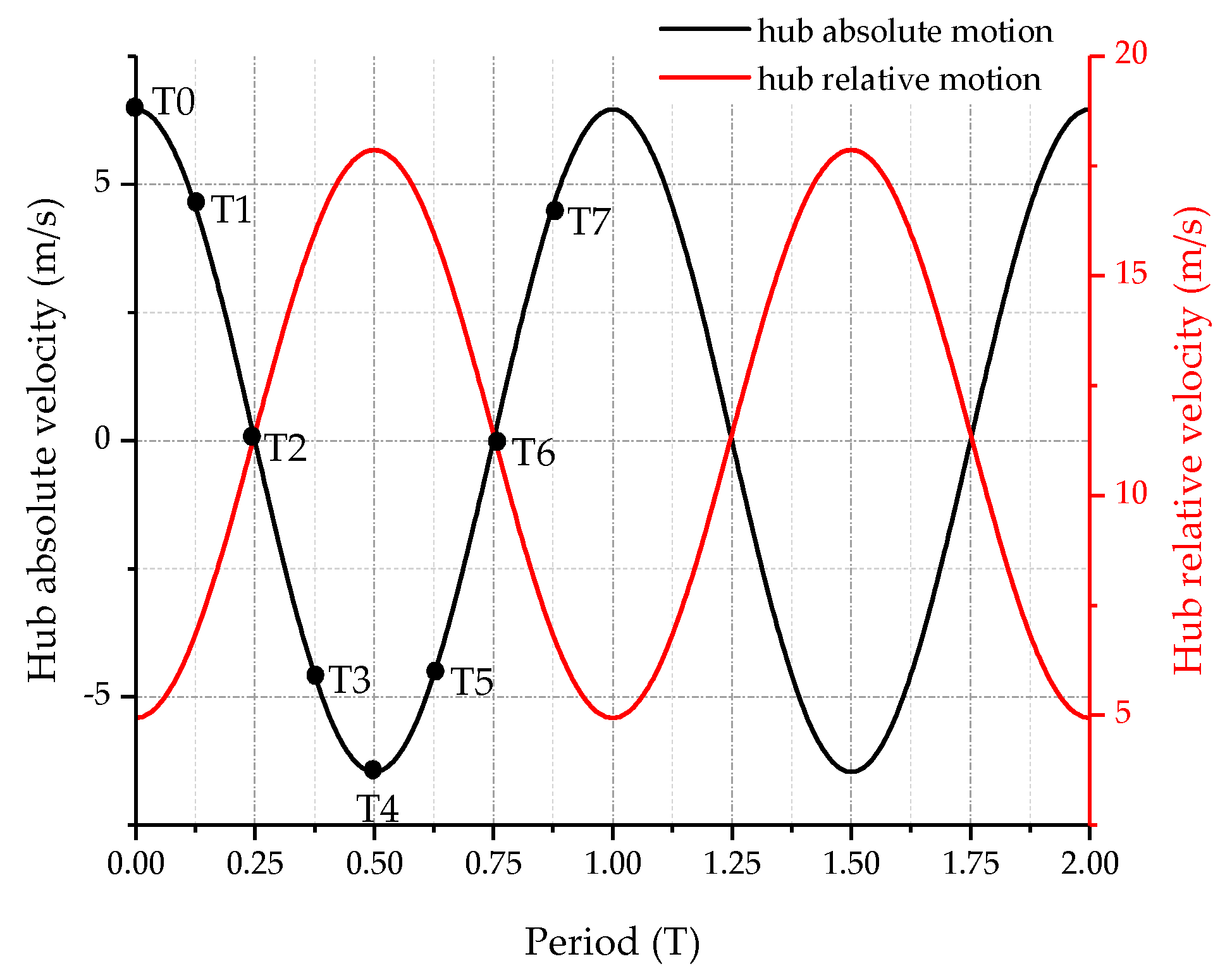
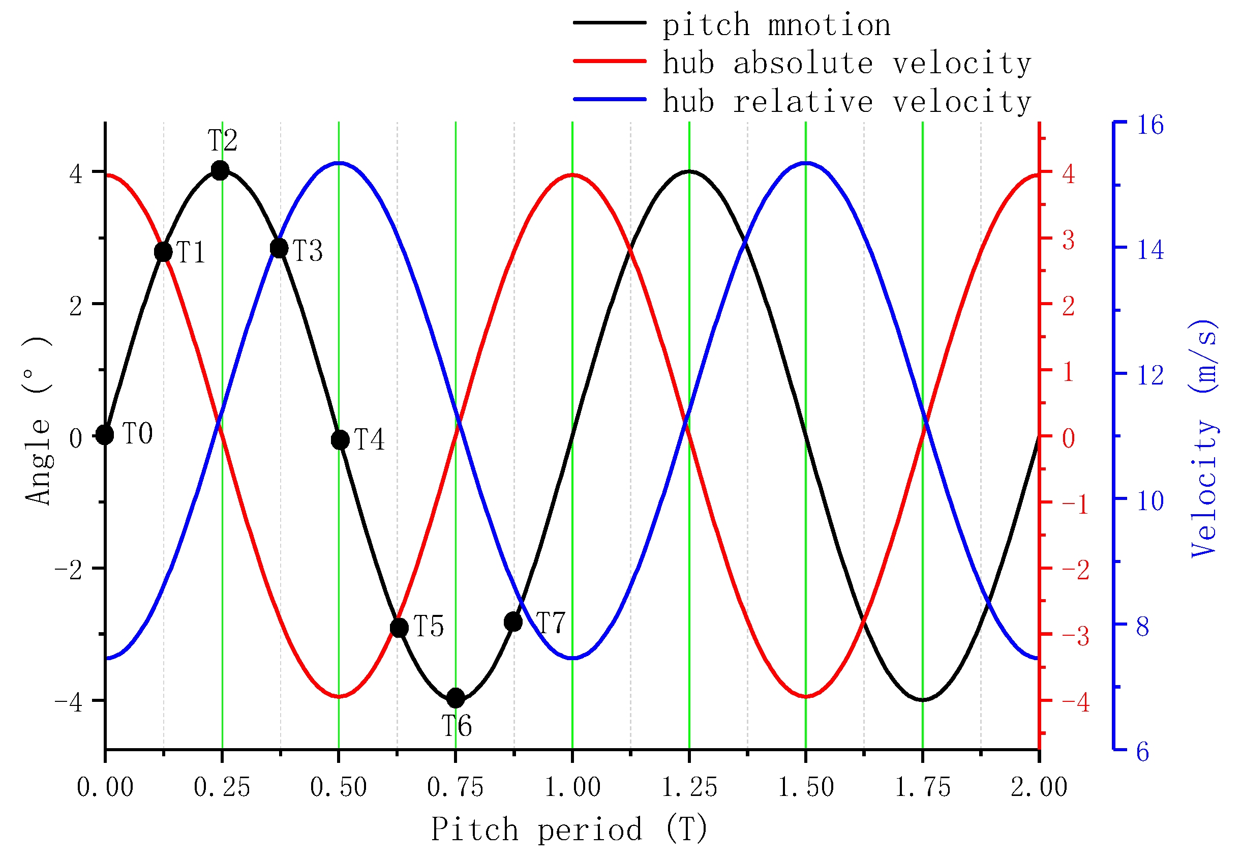
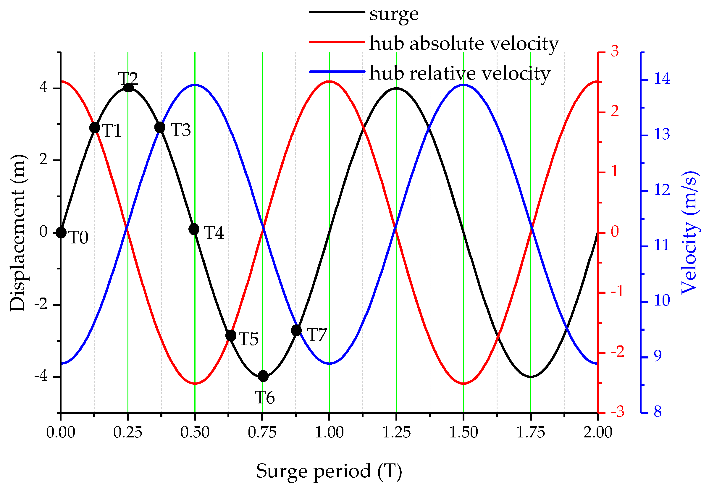
where $f$refers to the motion frequency, $H$ refers to the height of the hub above sea level. Figure 13 shows the combined motion under $A_P$= 4°, $A_S$= 4 m, $f$= 0.1 Hz. The absolute speed curve is shown in black, with the maximum absolute speed of approximately 6.46 m/s at T0 moment; the relative inflow wind speed at the hub is shown in red, with the maximum value of approximately 17.8 m/s at T4 moment. The simulation cases are the combination of single motion cases, as summarized in

Table 6. Cases of same-phase combined motion.

Case	Motion	${\mathit{A}}_{\mathit{P}}(°)$	${\mathit{A}}_{\mathit{S}}\left(\mathbf{m}\right)$	${\mathit{f}}_{\mathit{S}}\left(\mathbf{Hz}\right)$	${\mathit{P}}_{\mathit{m}} \left(\mathit{M}\mathit{W}\right)$	${\mathit{P}}_{+} \left(\mathit{M}\mathit{W}\right)$	$\mathit{\delta }$
11	Pitch + surge	1	1	0.1	4.94	6.84	37.35%
12	Pitch + surge	1	2	0.1	5.03	7.83	50.92%
13	Pitch + surge	2	1	0.1	5.11	8.08	57.78%
14	Pitch + surge	4	4	0.1	5.48	11.76	107.05%
15	Pitch + surge	1	1	0.2	5.12	8.92	69.20%
16	Pitch + surge	4	4	0.2	6.42	15.98	127.45%

.

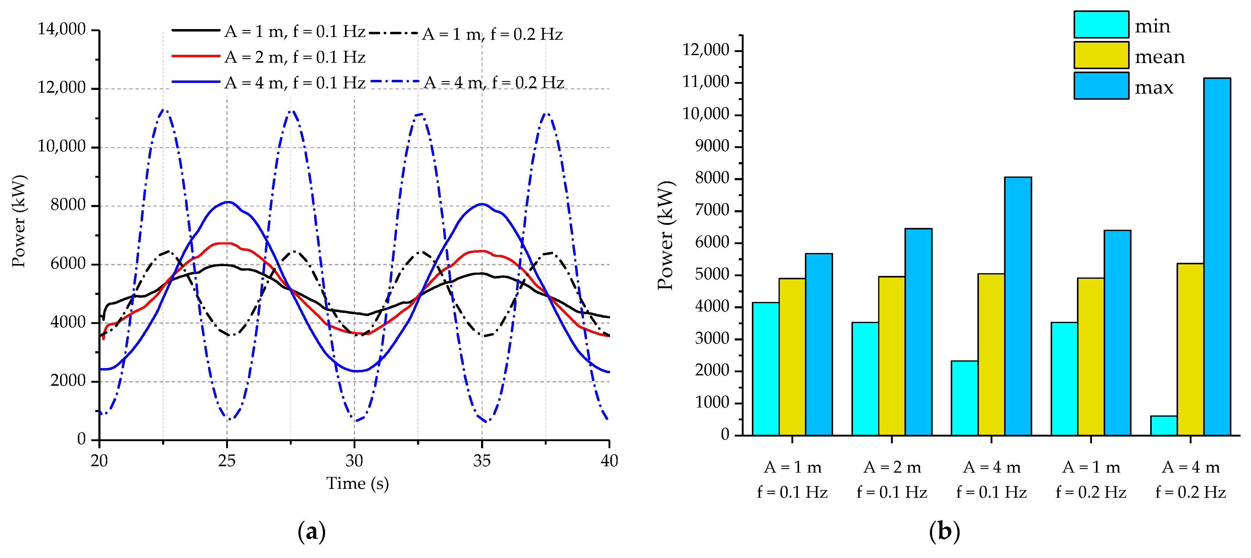
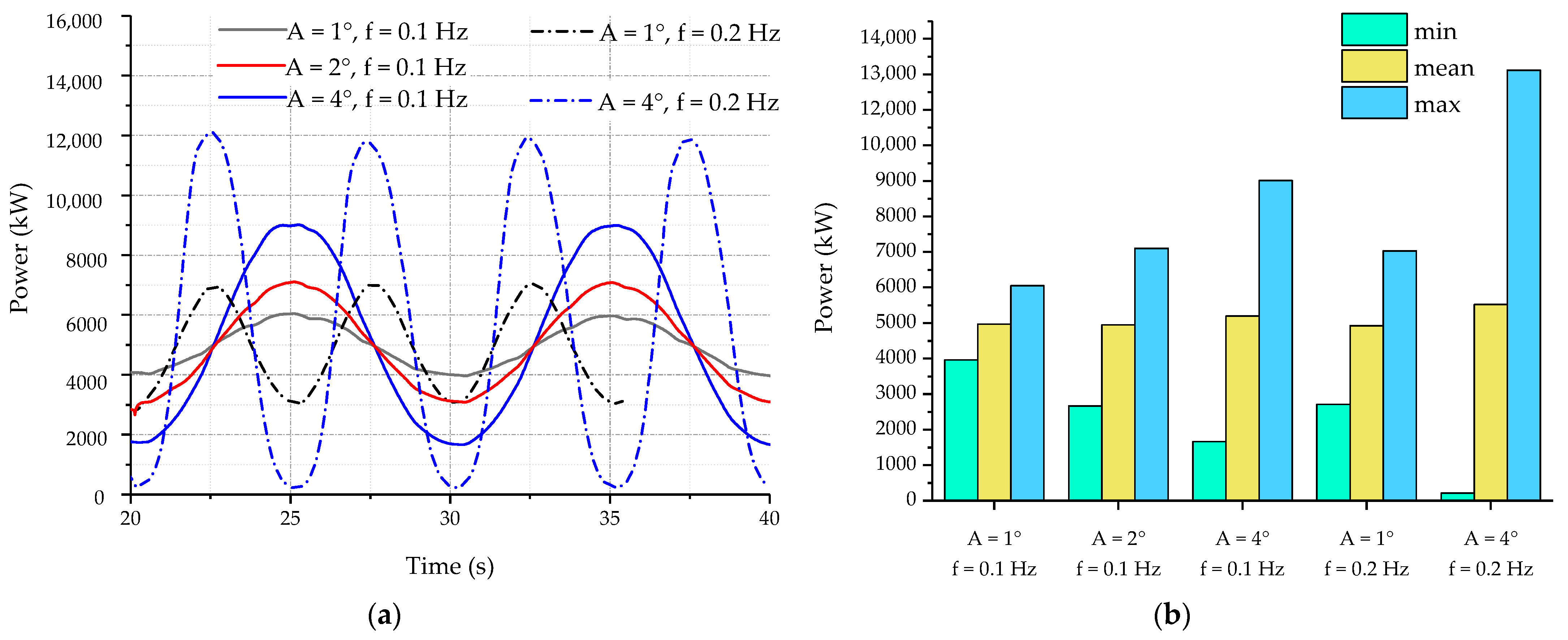
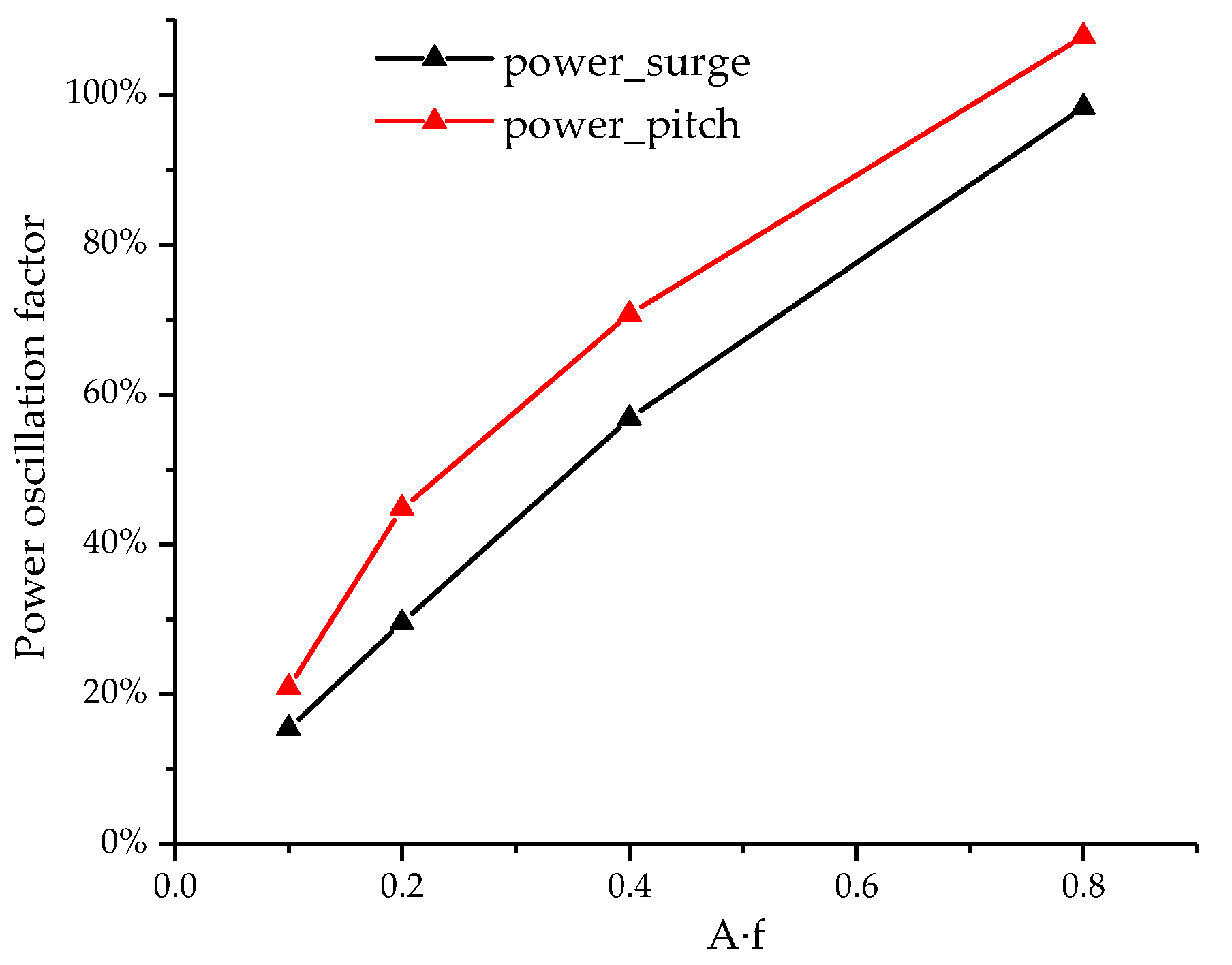
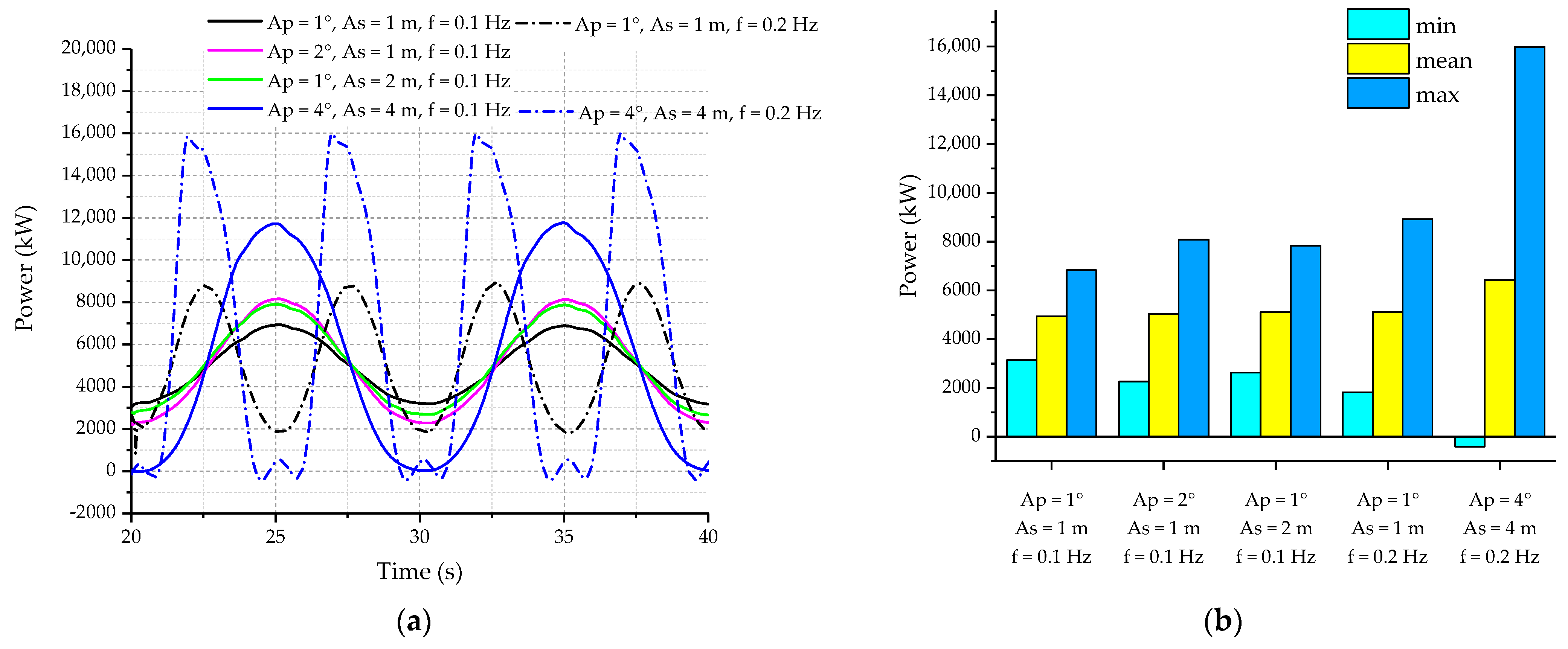
The wind turbine power under the same-phase combined motion is presented in Table 6 and Figure 14. One can notice that the same-phase combined motion aggravates the unsteady aerodynamic load characteristics of the wind turbine. The maximum power of combined motion is greater than that of either single motion under the same amplitude and frequency. The power oscillation factor of the combined motion is approximately equal to the algebraic sum of that of each sub-motion. Comparing the results of case 12 and case 13, it is obvious that the power oscillation under case 13 is more severe, which indicates that doubling the pitch amplitude has a greater impact than doubling the surge amplitude. Case 16 shows the occurrence of negative power, which is due to the negative relative inflow wind speed in this state.

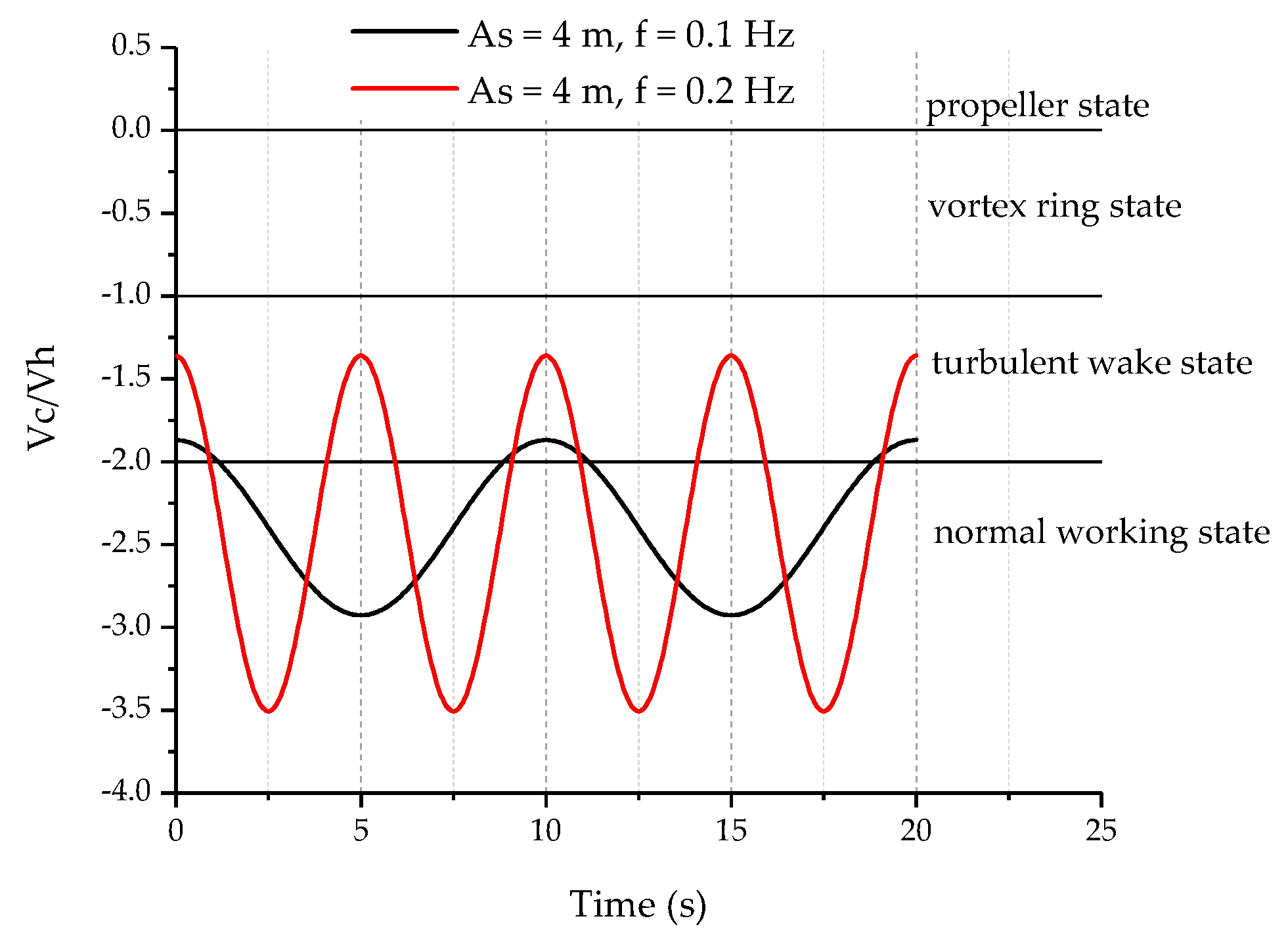
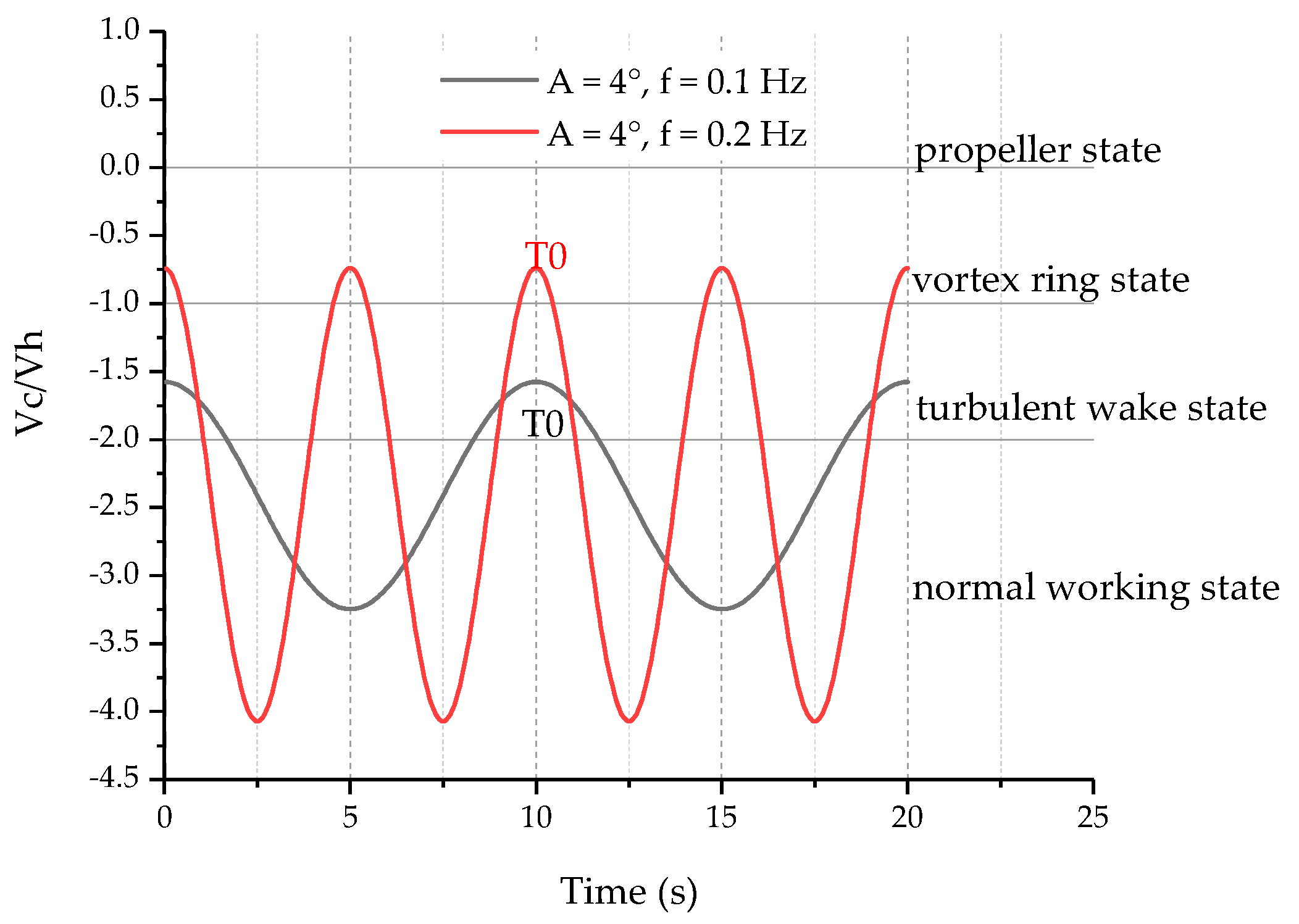
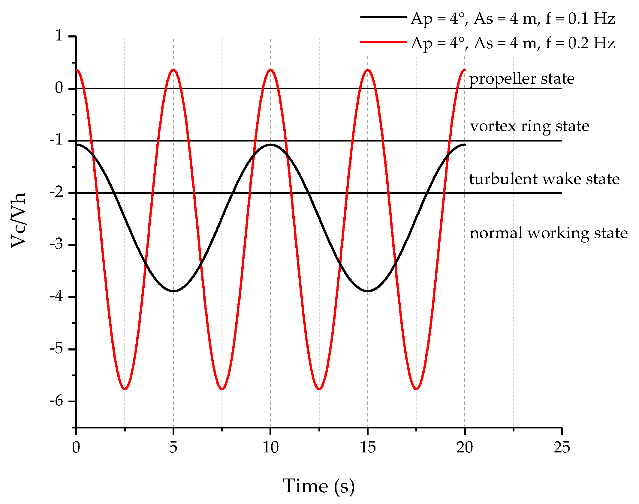
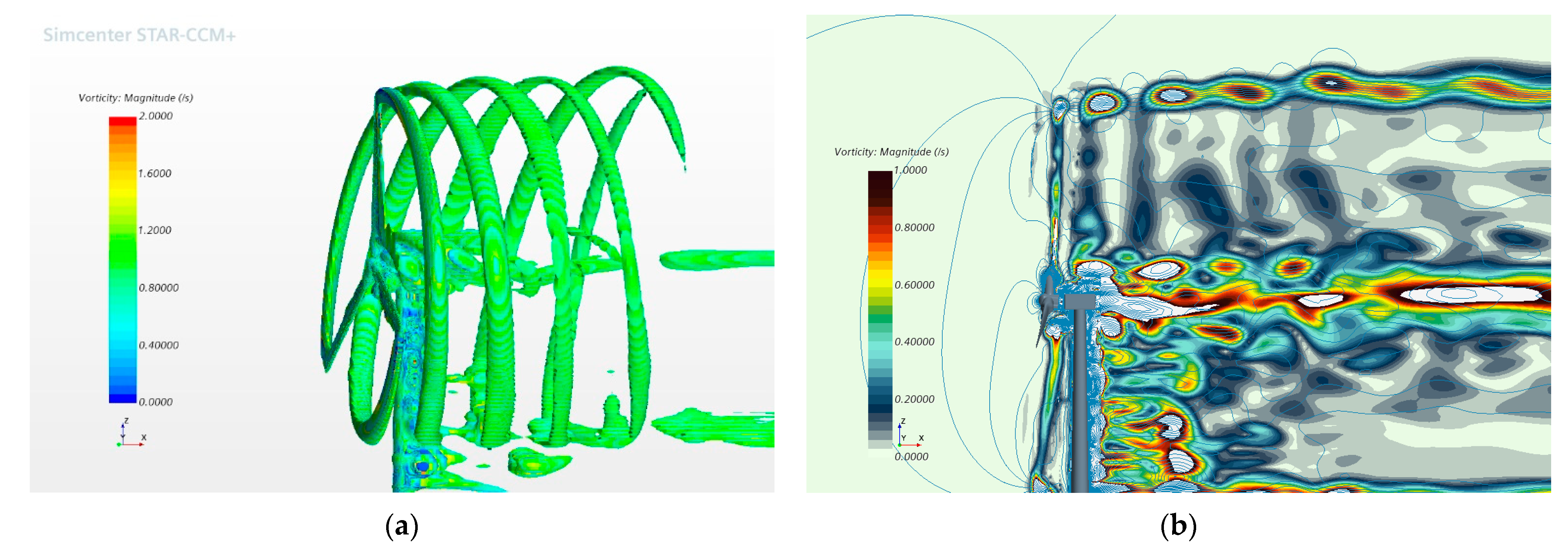
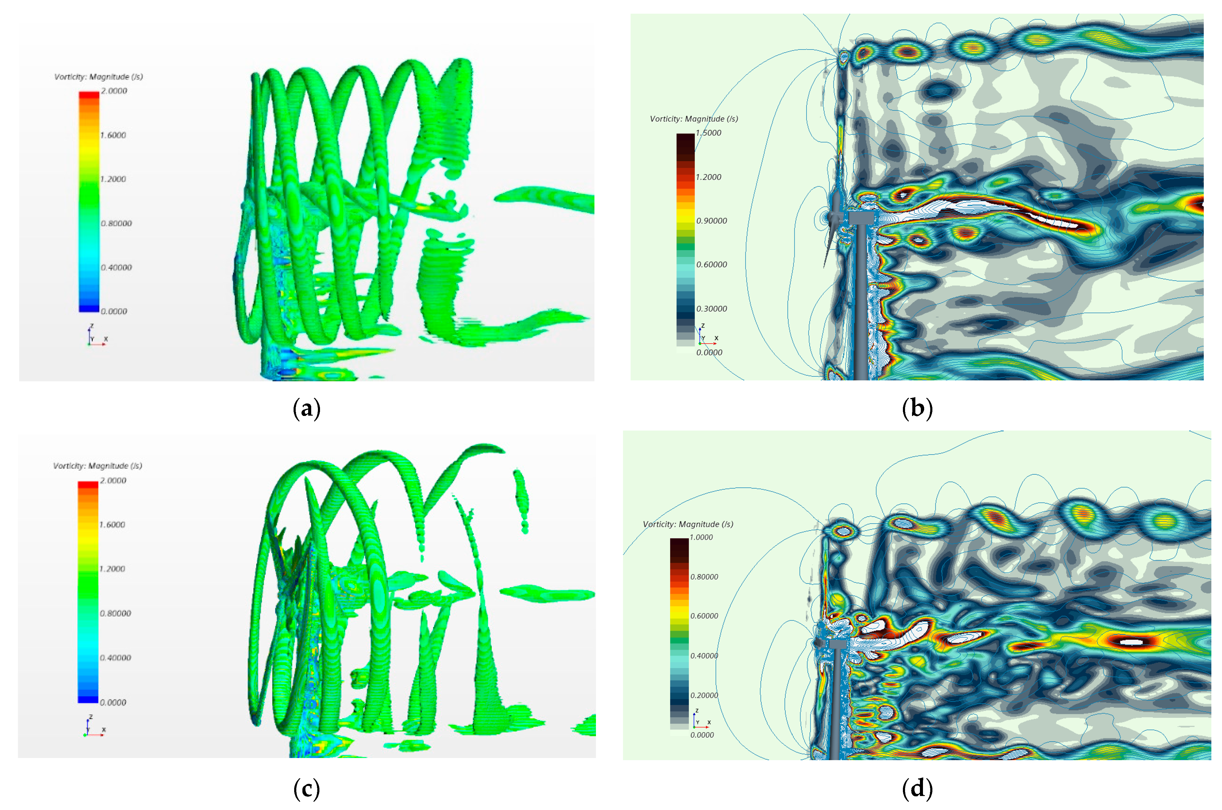
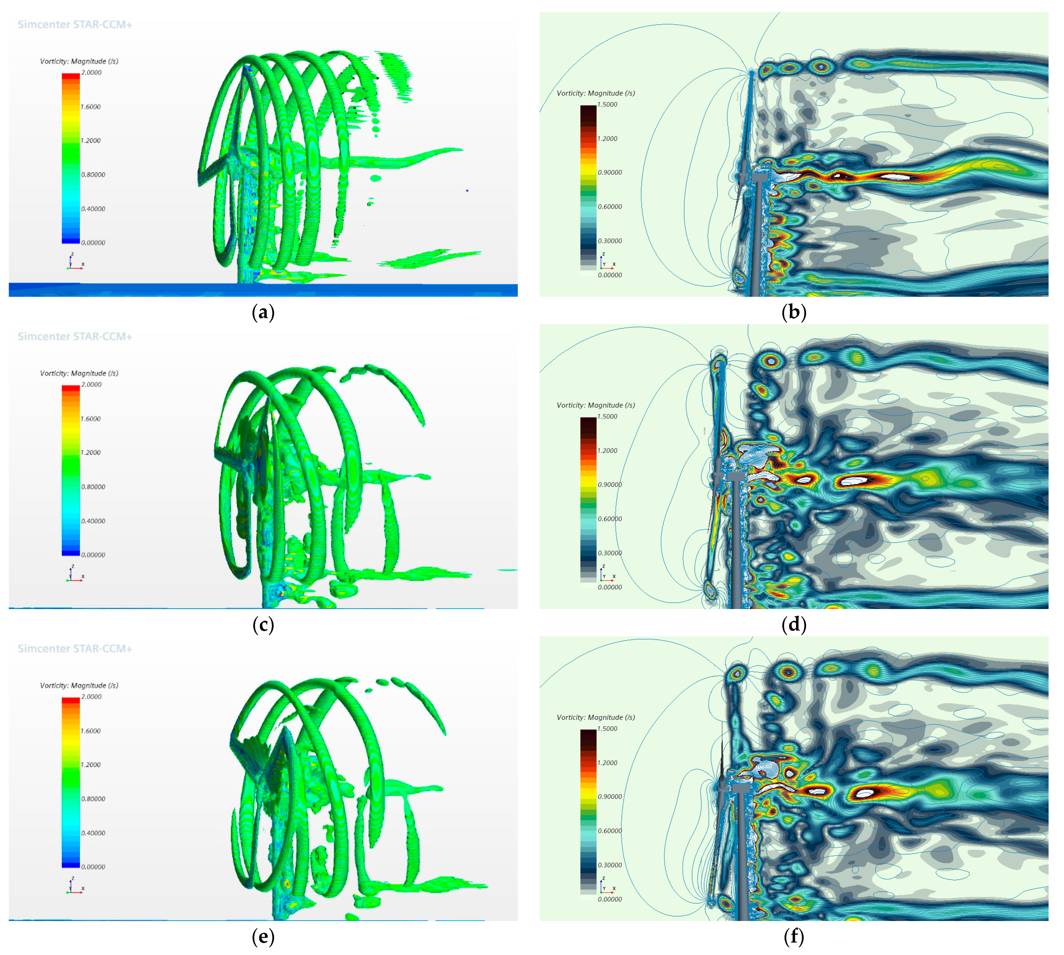
The speed ratio of case 14 and case 16 is shown in Figure 15. Under case 14 ($A_P=4°$, $A_S=4\mathrm{m}$, $f_S=0.1\mathrm{Hz}$), the wind turbine experiences two states and is on the edge of the vortex ring state. Under case 16 ($A_P=4°$, $A_S=4\mathrm{m}$, $f_S=0.2\mathrm{Hz}$), the wind turbine experiences four states. Figure 16 a,b depict the iso-surface of the vortex near the T0 moment under case 14. It is obvious that at T0, the gap between two vorticities is close to zero, which is coherent with the analysis results of Figure 15. The blades have strong turbulence effects but are not immersed in the wake vortex. 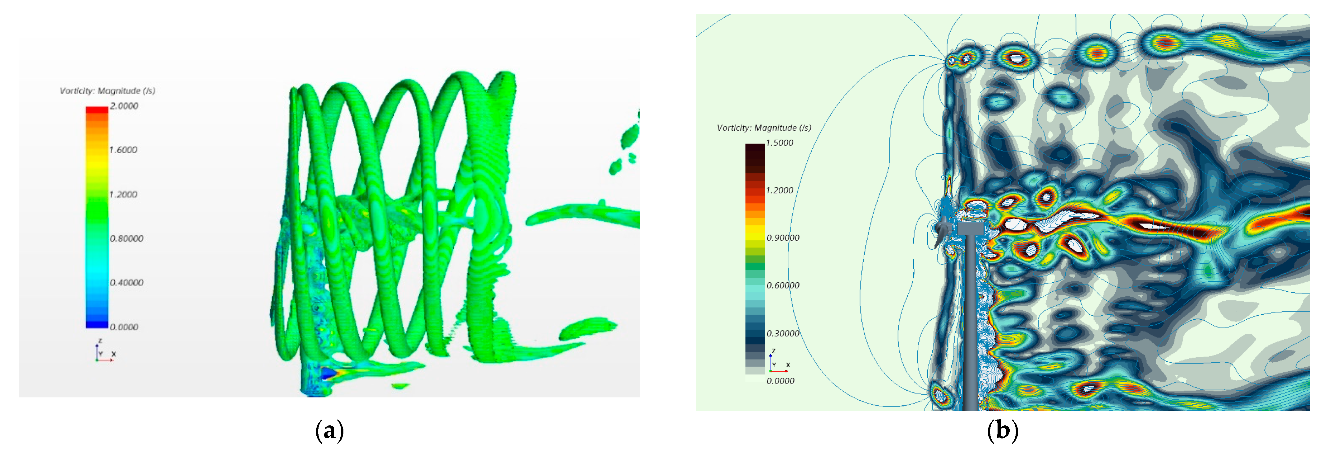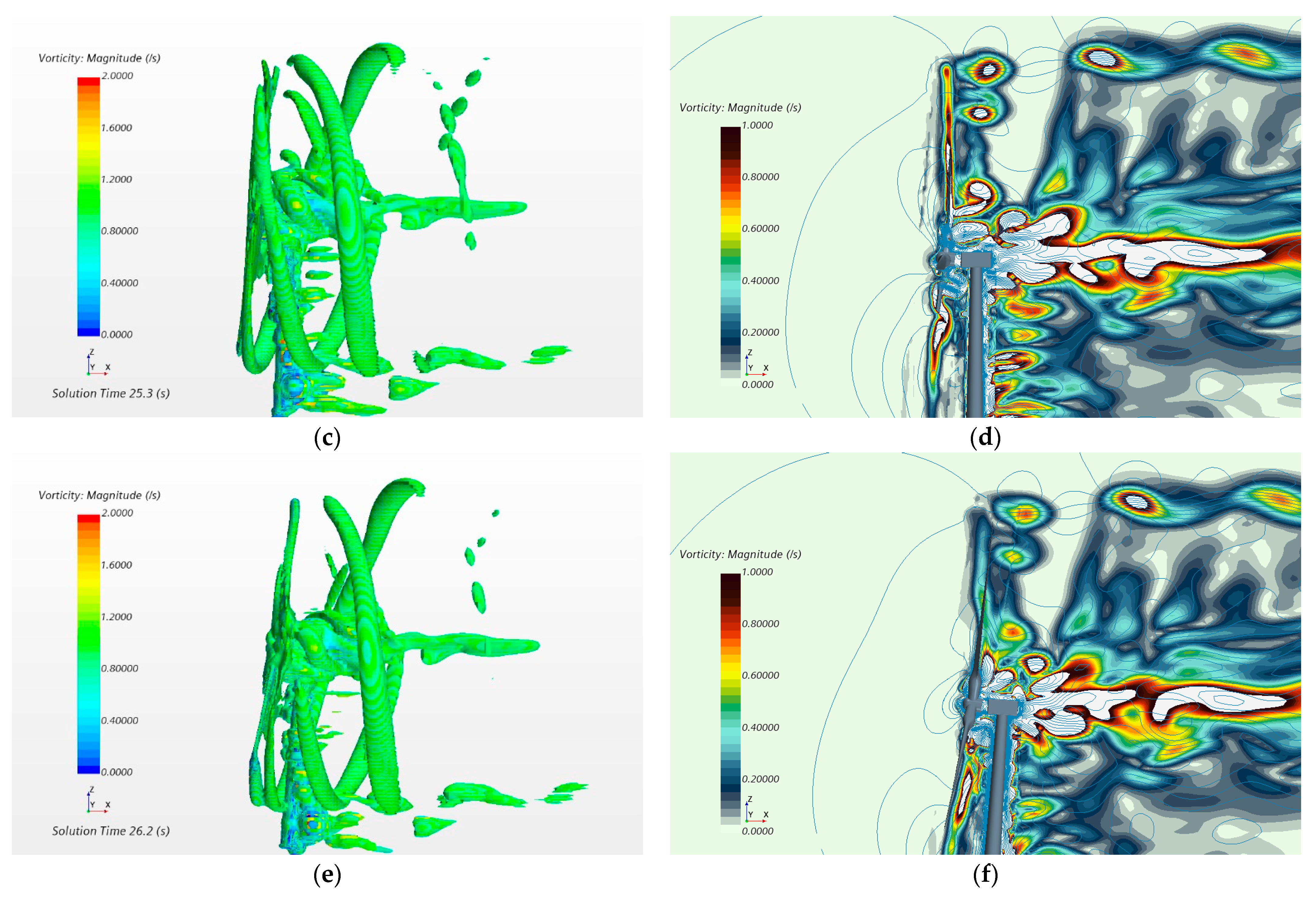Figure 16c–f show the iso-surface of the vortex near the T0 and T2 moment under case 16. There is a visible event of strong blade vortex interaction at the tip, as anticipated. The blade tip has entered the vortex generated by the previous blade and disturbed the normal development of the vortex. Figure 16c,e show that the wake vortex disturbed by the blade becomes extremely unstable, and then begins to break off and dissipate. Figure 16d,f on the right clearly show that the upcoming vortex enters the penult vortex domain as the previous vortex has been destroyed, and the vortex disappears soon after being disturbed.

4.2. Combined Motion with Phase Difference

Generally, there will be a constant phase difference between pitch and surge motion under steady wind and regular waves [28]. This steady-state phase difference comes from the phase difference between different wave excitation loads, and the phase difference between the excitation and response. At a certain wave frequency, the first-order wave excitation forces of surge and pitch DOFs can be expressed as:

$$F_x^{wave}=A_1\sin \left(\omega t+{\phi }_1\right)$$

(10)

$$M_y^{wave}=A_2\sin \left(\omega t+{\phi }_2\right)$$

(11)

The second-order hydrodynamics and coupling effects between motions are not considered in the following analysis. After linearization at the operating point, the surge and pitch motion can be considered as a second-order linear system with a single DOF, respectively [36]. According to the phase-frequency characteristics of the second-order linear system, the phase lag between the displacement response and the excitation force can be calculated through Equation (12) [37]:

$$\mathsf{\Delta }\psi =\arctan (-\frac{2\xi \lambda }{1-{\lambda }^2})$$

(12)

where $\lambda =\omega /{\omega }_n$ denotes frequency ratio, $\omega$is the excitation frequency, ${\omega }_n$ is the natural frequency; $\xi =c/2 m{\omega }_n$ denotes damping ratio, $c$ is the system damping, and $m$ is the mass or inertia.

Different types of floating platforms have different hydrodynamic characteristics and system inherent attributes. The platform in this paper refers to the OC4 semi-submersible floating platform designed by NREL [38]. The hydrodynamic characteristic parameters of the system, such as the wave excitation force and the radiation damping at different frequencies, can be obtained through frequency analysis in the ANSYS-AQWA software.

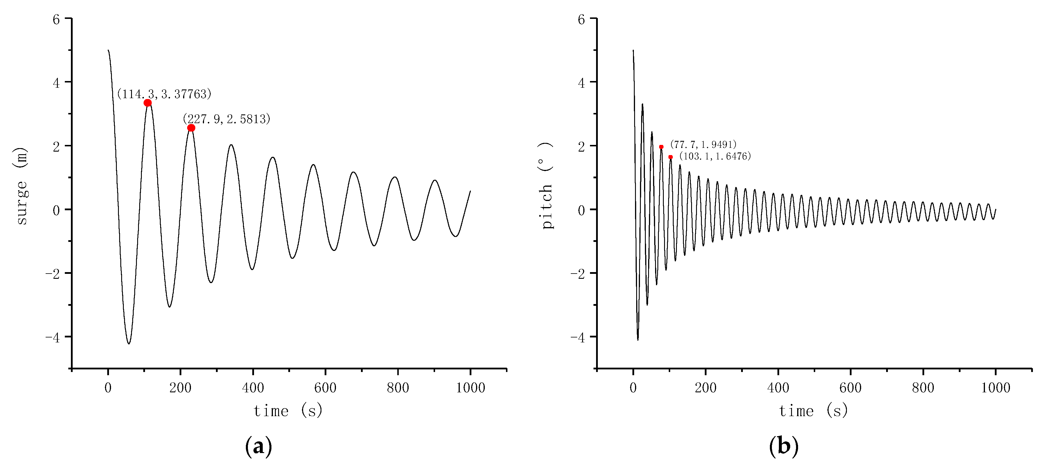
The natural frequency of the platform system can be obtained via the free decay test, as shown in Figure 17. The system response caused by the initial unit displacement has the following expression:

$$u\left(t\right)=e^{-\xi {\omega }_{n}t}(\cos {\omega }_{d}t+\frac{\xi }{\sqrt{1-{\xi }^2}}\sin {\omega }_{d}t)$$

(13)

The natural period of the system can be defined as follows:

$$T_n=T_d\sqrt{1-{\xi }^2}$$

(14)

where $T_d$ denotes the damping period, obtained through the points on the decay test curve. $\xi$ is the system damping (mainly fluid viscous damping as the radiation damping at the damping frequency is very small and can be ignored) and can be calculated by the Equation (15), where $\delta$ is the amplitude logarithmic decay rate, namely the natural logarithm of the ratio of two adjacent response amplitudes.

$$\xi \approx \frac{\delta }{2\mathsf{\pi }}=\frac{ln\frac{e^{-\xi {\omega }_{n}t}}{e^{-\xi {\omega }_n\left(t+T_d\right)}}}{2\mathsf{\pi }}$$

(15)

In addition, the system damping should also contain the aerodynamic damping. The linearization analysis was completed in OpenFAST v2.4.0 to obtain the aerodynamic damping values at the rated operating point [39].

Table 7. Damping parameters of the OC4 platform.

Parameters	Surge	Pitch
Natural frequency	0.0554 rad/s	0.2446 rad/s
Aerodynamic damping ratio	0.0513	0.1076
Radiation damping ratio	0.7665	0.07053
Viscous damping ratio	0.04279	0.01707
Total damping ratio	0.8606	0.1952

shows a summary of the system damping parameters at the rated wind speed operating point.

In the steady-state response of the system under the uniform wind and regular waves, the wind loads usually determine the equilibrium displacement, and the wave loads usually determine the oscillation amplitude of the system near the equilibrium point [29,40]. Taking a regular wave with a frequency of 0.1 Hz and a height of 2 m under the rated wind speed as an example, the phase analysis results are shown in

Table 8. Phase parameters of pitch and surge motions at 0.1 Hz.

Parameters	Surge	Pitch
Wave excitation force phase	69.9°	−87.4°
Total damping ratio	0.8606	0.1952
Frequency ratio	11.11	2.5688
Displacement phase (present)	−101.22	−259.42
Displacement phase (FAST 1)	−107	−264.5

¹ Fatigue, Aerodynamics, Structures, and Turbulence.

. It can be concluded from the table that the motion phase calculated according to Equation (12) is roughly consistent with the phase obtained by the FAST simulation results [39]. There is a certain discrepancy (about 6°), mainly due to model assumptions and inaccurate calculations of damping. Fortunately, the phase differences calculated by the two methods are almost equal with the discrepancy of 0.7°; therefore, the above method of calculating the phase difference is believable. For convenience, taking the surge motion as a reference, the phase difference of the pitch motion relative to the surge motion can be expressed as $\mathsf{\Delta }\psi ={\psi }_{pitch}-{\psi }_{surge}$. Then the absolute speed of the hub center is changed to:

$$V_H=2\mathsf{\pi }f\cdot H{A}_p\cdot \cos \left(2\mathsf{\pi }ft+\mathsf{\Delta }\psi \right)+2\mathsf{\pi }f\cdot A_s\cdot \cos (2\mathsf{\pi }ft)$$

(16)

According to the above analysis, each frequency uniquely determines the phase difference at a given wind speed; therefore, this paper selects two frequencies of 0.1 and 0.2 Hz as research. The specific simulation cases are shown in

Table 9. Cases of combined motion with phase difference.

Case	Motion	${\mathit{A}}_{\mathit{P}}(°)$	${\mathit{A}}_{\mathit{S}}\left(\mathbf{m}\right)$	$\mathit{f}$	$\mathit{\Delta }\mathit{\psi }{ }^1$	${\mathit{P}}_{\mathit{m}} \left(\mathit{M}\mathit{W}\right)$	${\mathit{P}}_{+} \left(\mathit{M}\mathit{W}\right)$	$\mathit{\delta }$
17	Pitch + surge	1	1	0.1	−158.2°	4.92	5.42	10.66%
18	Pitch + surge	1	2	0.1	−158.2°	4.91	5.49	11.11%
19	Pitch + surge	2	1	0.1	−158.2°	4.97	6.57	31.66%
20	Pitch + surge	4	4	0.1	−158.2°	4.92	7.10	40.69%
21	Pitch + surge	1	1	0.2	−270°	4.98	7.69	52.16%
22	Pitch + surge	4	4	0.2	−270°	5.57	14.24	131.38%

¹ Phase difference.

. Figure 18a,b show the motions of the wind turbine under case 20 and case 22, respectively. Under case 20, the moment of maximum absolute speed of the hub center moves to T3. Under case 22, the moment of maximum absolute speed moment moves to T7.

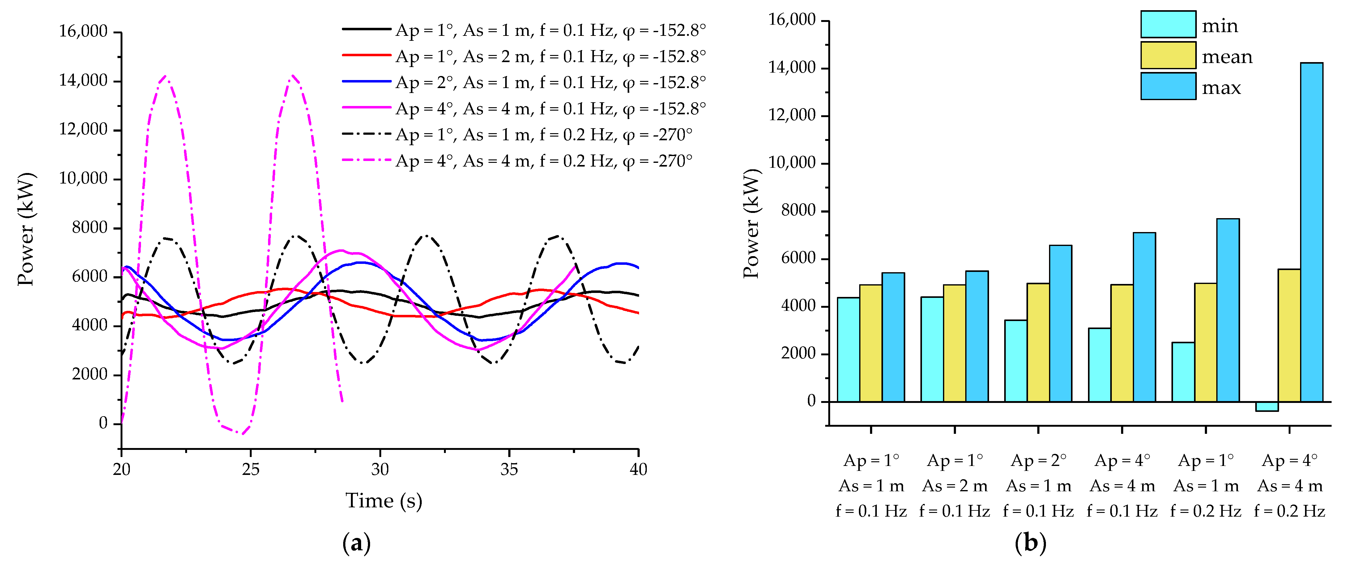
Under the combined motion with a phase difference, the power variation curves are depicted in Figure 19, and the power statistics are presented in Table 9. First, the power oscillation under the combined motion with a phase difference is smaller than that under the same-phase combined motion. The maximum power of case 17 is reduced by 1.42 MW compared to case 11, and the maximum power of case 21 is reduced by 1.23 MW compared to case 15. It is concluded that the impact on the attenuation of power at 0.1 Hz is greater than that at 0.2 Hz. Furthermore, under different frequencies, the combined motion with phase difference has different power influence characteristics compared to the single motion. At 0.1 Hz, the maximum power of case 17 is smaller than that of the pitch motion of case 1 and the surge motion of case 6; however, at 0.2 Hz, the maximum power of case 20 is larger than that of the pitch motion of case 4 and the surge motion of case 9. This illustrates the mutual weakening effects on power characteristics between pitch and surge motion at 0.1 HZ and the mutual strengthening effects at 0.2 HZ. In addition, under combinations of different motion amplitudes, the characteristic position of the power variation curve is different. At 0.1 Hz, the maximum power occurs near the T7 moment in case 17, near the T5 moment in case 18, and near the T7~T0 moment in case 19. This is mainly because the power is affected by pitch and surge motion amplitude differently.

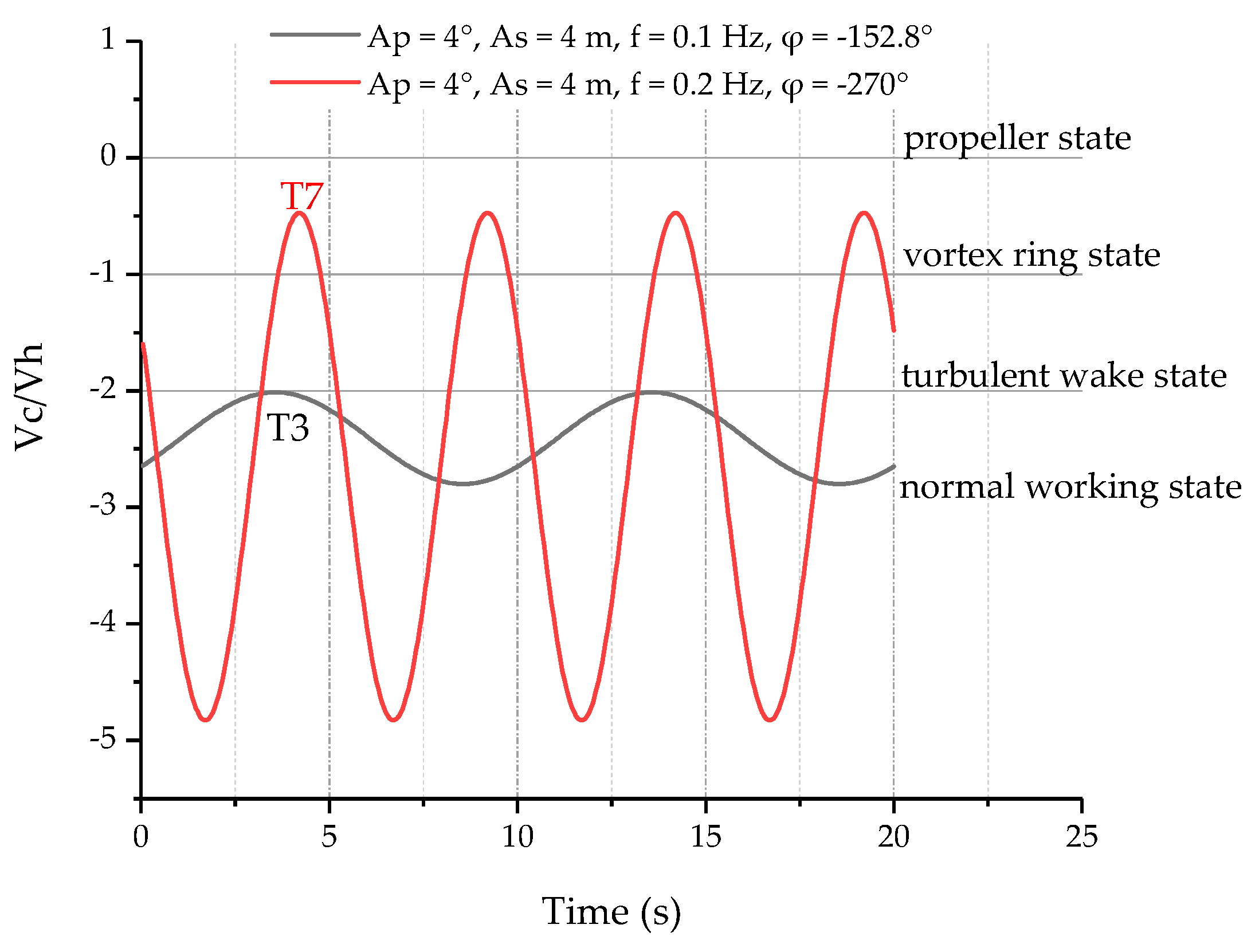
The speed ratio $V_c/V_h$ of case 20 and case 22 are shown in Figure 20. The wind turbine under case 20 is only in the normal working state, whereas it experiences three states except the propeller state under case 22; however, case 22 shows a negative power phenomenon in Figure 19 as the hub speed used in the formula $V_c/V_h$ cannot represent the speed distribution of the whole rotor plane.

Figure 21a,b display the iso-surface of the vortex at T3 moment under case 20. The gap between wake vortices shedding from the blade tip maintains a certain distance, which is different from case 14. It is visible that the blade does not directly interfere with the wake vortex. Figure 21c–f display the iso-surface of the vortex under case 22. The vortex emitted by the previous blade has been stroke by the next blade before it flows downstream away from the tip near the T7 moment. The wind turbine has completely entered the vortex ring state, but the intensity of blade/vortex interference is reduced, and the integrity of the vortex structure is better than in case 16. The blade breaks away from its own wake vortices for a while; then, new wake vortices are generated based on the previous one, so what we see is that no new vortex structure is produced during this time.

5. Motion Induced by Real Sea States

The motion amplitude given in Section 3 and Section 4 is an ideal choice for the convenience of comparative analysis. In order to reflect the load fluctuations of the turbine under real sea conditions, the reasonable possible motion amplitude of the wind turbine was selected based on the sea state data of Shidao in China from 1996 to 2020. Figure 22 shows the distribution probability of meteorological conditions; the significant wave height is mainly distributed between 0.5 and 1.0 m, the zero-crossing period is mainly distributed in 4–7 s, and the wind speed is mainly distributed in the low wind speed region. Response amplitude operator (RAO), which can be obtained through the ANSYS-AQWA software, is used to predict the response of the FOWT under a given sea state. RAO is defined as follows:

$$RA{O}_i\left(\omega \right)=\frac{A_{motion}}{A_{wave}} i=1,5$$

(17)

where $A_{motion}$ refers to the response amplitude, $A_{wave}$ refers to wave amplitude, and $i=1, 5$ denotes the surge and pitch motion, respectively. The FOWT response amplitude can be calculated when given the wave period and wave amplitude. Generally, the significant height has the following relationship to wave amplitude [41]:

$$A_{wave}^2=\frac{H_s^2}{8}$$

(18)

According to Equations (17) and (18) and the phase difference analysis method in Section 4, one can establish the motion table as the function of wave parameters, as shown in

Table 10. Motion states at given sea states.

Tp (s)	Hs (m)	${\mathit{A}}_{\mathit{P}}(°)$	${\mathit{f}}_{\mathit{P}}\left(\mathbf{Hz}\right)$	${\mathit{A}}_{\mathit{S}}\left(\mathbf{m}\right)$	${\mathit{f}}_{\mathit{S}}\left(\mathbf{m}\right)$	$\Delta \mathit{\psi } (°){}^1$
5	0.5	0.0022	0.2	0.0266	0.2	−270
5	1.0	0.0044	0.2	0.05751	0.2	−270
5	3.0	0.01284	0.2	0.1734	0.2	−270
10	0.5	0.0893	0.1	0.09727	0.1	−158.2
10	1.0	0.1788	0.1	0.1959	0.1	−158.2
10	3.0	0.5377	0.1	0.5894	0.1	−158.2

¹ Phase difference.

. It should be emphasized here that all phase differences are calculated with the aerodynamic damping value at the rated wind speed for simplicity. The motion amplitude increases with the increment of the wave period and the significant height. The pitch motion amplitude does not exceed 1°, the maximum value in the table is only 0.5377°, and the maximum surge oscillation is only 1.105 m in this sea area.

Considering that the rotor has large inertia and the wave period is short, one can assume that the rotor speed does not change during such a period. The statistical results of power variation under different sea conditions are shown in

Table 11. The power fluctuation value at the given environment; units are in kW.

Tp (s)	Hs (m)	v (m/s)
		5	8	11.4	15
5	0.5	18.57	39.48	71.25	76.51
5	1.0	37.63	80.3	145.3	155.1
5	3.0	143.37	245.8	438	479.9
10	0.5	15.27	34.82	61.58	66.6
10	1.0	31.14	67.84	115.6	131.4
10	3.0	89.45	192.5	343.3	375.2
15	0.5	13.27	28.8	54.83	56.85
15	1.0	25.99	57.11	105.1	111.5
15	3.0	75.32	167.6	303.7	326.7

. In this sea area, the power increases with the increase of wind speed and significant wave height but decreases with the increase of the period. The maximum power fluctuation amplitude is 479.9 KW.

6. Conclusions

Based on STAR-CCM+, we conducted the unsteady numerical simulation of the NREL 5-MW wind turbine and investigated the power performance and the wake structure under different platform motions. In particular, the simulations under platform motions with a phase difference, which other scholars did not consider before, were performed through the proposed approach in this paper. These research results help to better understand the influence law of platform motions on power performance, and provide new ideas and directions for the CFD simulation of wind turbines under multi-DOFs motions. In addition, simulations under realistic platform motions were conducted in the given environment. These simulation results will be more practically useful than the simulation results in which ideal motion amplitudes were used. The main conclusions are drawn as follows:

• As the motion amplitude or frequency increases under the single motion, the average power increases slightly and the power fluctuation aggravates heavily. The power performance of wind turbines is more susceptible to pitch than surge motion.
• The power oscillation under the same-phase combined motion is more severe than that under a single motion. The wind turbine under the same-phase combined motion is more likely to enter the propeller state.
• The combined motion with phase difference has different influence effects on the power performances at different frequencies. At 0.1 Hz, the power oscillation factor is smaller than that under the single motion; at 0.2 Hz, the power oscillation factor is larger than that under the single motion but still smaller than that under the same-phase combined motion. Furthermore, different combinations of motion amplitudes will alter the characteristic position of power variation.
• Under most real sea conditions in Shidao in China, the maximum pitch oscillation amplitude of the platform is only 0.5377°, the maximum surge oscillation amplitude is only 1.105 m, and the maximum power fluctuation amplitude is 479.9 kW.

In the future, the research will extend the simulations to more complex motions by adding yaw motion as a further DOF. Moreover, an improved approach to calculating phase difference will be proposed by considering the coupling effects between motions. In addition, the power variation table will be constructed based on wind-wave joint distribution probability.

References

1. Global Wind Report. 2021. Available online: https://gwec.net/global-wind-report-2021/ (accessed on 25 March 2021).
2. Liu, Y.; Li, S.; Yi, Q. Developments in semi-submersible floating foundations supporting wind turbines: A comprehensive review. Renew. Sustain. Energ. Rev. 2016, 60, 433–449. [Google Scholar] [CrossRef]
3. Jiang, Z. Installation of offshore wind turbines: A technical review. Renew. Sustain. Energ. Rev. 2021, 139, 110576. [Google Scholar] [CrossRef]
4. Xu, K.; Larsen, K.; Shao, Y. Design and comparative analysis of alternative mooring systems for floating wind turbines in shallow water with emphasis on ultimate limit state design. Ocean Eng. 2021, 219, 108377. [Google Scholar] [CrossRef]
5. Sebastian, T.; Lackner, M.A. Characterization of the unsteady aerodynamics of offshore floating wind turbines. Wind Energy 2013, 16, 339–352. [Google Scholar] [CrossRef]
6. Jonkman, J.M. Dynamics of offshore floating wind turbines-model development and verification. Wind Energy 2009, 12, 459–492. [Google Scholar] [CrossRef]
7. Jonkman, J.M.; Matha, D. Dynamics of offshore floating wind turbines-analysis of three concepts. Wind Energy 2011, 14, 557–569. [Google Scholar] [CrossRef]
8. De Vaal, J.B.; Hansen, M.O.L.; Moan, T. Effect of wind turbine surge motion on rotor thrust and induced velocity. Wind Energy 2014, 17, 105–121. [Google Scholar] [CrossRef]
9. Tran, T.; Kim, D. The platform pitching motion of floating offshore wind turbine: A preliminary unsteady aerodynamic analysis. J. Wind Eng. Ind. Aerodyn. 2015, 142, 65–81. [Google Scholar] [CrossRef] [Green Version]
10. Wen, B.; Dong, X.; Tian, X. The power performance of an offshore floating wind turbine in platform pitching motion. Energy 2018, 154, 508–521. [Google Scholar] [CrossRef]
11. Wen, B.; Tian, X.; Dong, X. Influences of surge motion on the power and thrust characteristics of an offshore floating wind turbine. Energy 2017, 141, 2054–2068. [Google Scholar] [CrossRef]
12. Farrugia, R.; Sant, T.; Micallef, D. A study on the aerodynamics of a floating wind turbine rotor. Renew. Energy 2016, 86, 770–784. [Google Scholar] [CrossRef]
13. Jeon, M.; Lee, S.; Lee, S. Unsteady aerodynamics of offshore floating wind turbines in platform pitching motion using vortex lattice method. Renew. Energy 2014, 65, 207–212. [Google Scholar] [CrossRef]
14. Tran, T.; Kim, D.; Song, J. Computational Fluid Dynamic Analysis of a Floating Offshore Wind Turbine Experiencing Platform Pitching Motion. Energies 2014, 7, 5011–5026. [Google Scholar] [CrossRef]
15. Tran, T.; Kim, D. The aerodynamic interference effects of a floating offshore wind turbine experiencing platform pitching and yawing motions. J. Mech. Sci. Technol 2015, 29, 549–561. [Google Scholar] [CrossRef]
16. Leble, V.; Barakos, G. 10-MW Wind Turbine Performance under Pitching and Yawing Motion. J. Sol. Energy Eng. 2017, 139, 041003. [Google Scholar] [CrossRef]
17. Lienard, C.; Boisard, R.; Daudin, C. Aerodynamic behavior of a floating offshore wind turbine. In Proceedings of the AIAA Scitech 2019 Forum, San Diego, CA, USA, 7–11 January 2019. [Google Scholar]
18. Kyle, R.; Lee, Y.C.; Früh, W. Propeller and vortex ring state for floating offshore wind turbines during surge. Renew. Energy 2020, 155, 645–657. [Google Scholar] [CrossRef]
19. Chen, Z.; Wang, X.; Guo, Y. Numerical analysis of unsteady aerodynamic performance of floating offshore wind turbine under platform surge and pitch motions. Renew. Energy 2021, 163, 1849–1870. [Google Scholar] [CrossRef]
20. Wu, C.K.; Nguyen, V. Aerodynamic simulations of offshore floating wind turbine in platform-induced pitching motion. Wind Energy 2017, 20, 835–858. [Google Scholar] [CrossRef]
21. Rockel, S.; Camp, E.; Schmidt, J. Experimental Study on Influence of Pitch Motion on the Wake of a Floating Wind Turbine Model. Energies, 2014, 7, 1954–1985. [Google Scholar] [CrossRef] [Green Version]
22. Rockel, S.; Peinke, J.; Hölling, M. Wake to wake interaction of floating wind turbine models in free pitch motion: An eddy viscosity and mixing length approach. Renew. Energy 2016, 85, 666–676. [Google Scholar] [CrossRef]
23. Fu, S.; Jin, Y.; Zheng, Y. Wake and power fluctuations of a model wind turbine subjected to pitch and roll oscillations. Appl. Energy 2019, 253, 113605. [Google Scholar] [CrossRef]
24. Hu, H.; Khosravi, M.; Sarkar, P. An Experimental Investigation on the Aeromechanic Performance and Wake Characteristics of a Wind Turbine Model Subjected to Pitch Motions. In Proceedings of the 34th Wind Energy Symposium, San Diego, CA, USA, 4–8 January 2016. [Google Scholar]
25. Bayati, I.; Belloli, M.; Bernini, L. Wind tunnel validation of AeroDyn within LIFES50+ project: Imposed Surge and Pitch tests. J Phys. Conf. Ser. 2016, 753, 092001. [Google Scholar] [CrossRef]
26. Sebastian, T.; Lackner, M.A. Development of a free vortex wake method code for offshore floating wind turbines. Renew. Energy 2012, 46, 269–275. [Google Scholar] [CrossRef]
27. Sebastian, T.; Lackner, M.A. Analysis of the Induction and Wake Evolution of an Offshore Floating Wind Turbine. Energies 2012, 5, 968–1000. [Google Scholar] [CrossRef] [Green Version]
28. Cheng, P.; Huang, Y.; Wan, D. A numerical model for fully coupled aero-hydrodynamic analysis of floating offshore wind turbine. Ocean Eng. 2019, 173, 183–196. [Google Scholar] [CrossRef]
29. Jonkman, J.; Butterfield, S.; Musial, W.; Scott, G. Definition of a 5-MW Reference Wind Turbine for Offshore System Development. Technical Report NREL/TP-500–38060; National Renewable Energy Laboratory: Golde, CO, USA, 2009.
30. Sebastian, T. The Aerodynamic and Near Wake of an Offshore Floating Horizontal Axis Wind Turbine. Ph.D. Thesis, University of Massachusetts, Amherst, MA, USA, 2012. [Google Scholar]
31. Gupta, S.; Leishman, J. Comparison of Momentum And Vortex Methods For The Aerodynamic Analysis Of Wind Turbines. In Proceedings of the 43rd AIAA Aerospace Sciences Meeting and Exhibit, Reno, NV, USA, 10–13 January 2005. [Google Scholar]
32. Menter, F.R. Review of the shear-stress transport turbulence model experience from an industrial perspective. Int. J. Comput. Fluid Dyn. 2009, 23, 305–316. [Google Scholar] [CrossRef]
33. STAR-CCM+ Help Manual. 2021. Available online: http://starccm.sourceforge.net/ (accessed on 25 May 2021).
34. Wu, J.; Ding, J.; He, Y.; Zhao, Y. Study on unsteady aerodynamic performance of floating offshore wind turbine by CFD method. In Proceedings of the 25th International Offshore and Polar Engineering Conference, Kona, HI, USA, 21–26 June 2015; pp. 554–560. [Google Scholar]
35. Leble, V.; Barakos, G. Rigid Actuation of the Wind Turbine. In Proceedings of the 72nd Annual Forum of the American Helicopter Society, Palm Beach, FL, USA, 17–19 May 2016. [Google Scholar]
36. Li, Y.; Li, W.; Liu, H. Indirect load measurements for large floating horizontal-axis tidal current turbines. Ocean Eng. 2020, 198, 106945. [Google Scholar] [CrossRef]
37. Thomson, W.T. Theory of Vibration with Applications, 2nd ed.; Prentice-Hall, Inc.: Englewood Cliffs, NJ, USA, 1981; p. 50. [Google Scholar]
38. Coulling, A.J.; Goupee, A.J.; Robertson, A.N. Validation of a FAST semi-submersible floating wind turbine numerical model with DeepCwind test data. J. Renew. Sustain. Energy 2013, 5, 23116. [Google Scholar] [CrossRef]
39. Jonkman, J.; Buhl, M. FAST User’s Guide. Technical Report NREL/EL-500–38230; National Renewable Energy Laboratory: Golde, CO, USA, 2005.
40. Liu, Y.; Xiao, Q.; Incecik, A. Establishing a fully coupled CFD analysis tool for floating offshore wind turbines. Renew. Energy 2017, 112, 280–301. [Google Scholar] [CrossRef] [Green Version]
41. Sørensen, W.T. Renewable Energy: Its Physics, Engineering, Use, Environmental Impacts, Economy and Planning Aspects, 3rd ed.; Elsevier Academic Press: San Diego, CA, USA, 2004; pp. 256–257. [Google Scholar]
Figure 1. Six DOFs motions for a floating offshore wind turbine.
Jmse 09 00699 g001
Figure 2. Simulated mesh in different parts. (a) The full fluid domain; (b) blade surface mesh; (c) overset mesh; (d) hub surface mesh.
Jmse 09 00699 g002
Figure 3. Power coefficient comparison results. (a) Pitch motion with amplitude of 1° and frequency of 0.1 Hz; (b) surge motion with an amplitude of 2 m and a frequency of 0.1 Hz.
Jmse 09 00699 g003
Figure 4. Pitch motion analysis under case 3 ( A P = 4 ° ,   f P = 0.1   Hz ).
Jmse 09 00699 g004
Figure 5. Power performance under pitch motion. (a) Power variation versus time; (b) the average and extreme power.
Jmse 09 00699 g005
Figure 6. VRS identification scheme under pitch motion.
Jmse 09 00699 g006
Figure 7. Wake scheme under pitch motion. (a) Iso-surface at T0 moment under case 3; (b) velocity in the symmetry plane at T0 moment under case 3; (c) iso-surface at T0 moment under case 5; (d) velocity in the symmetry plane at T0 moment under case 5.
Jmse 09 00699 g007
Figure 8. Surge motion analysis under case 10 ( A S = 4   m ,   f S = 0.1   Hz ).
Jmse 09 00699 g008
Figure 9. Power performance under surge motion. (a) Power variation versus time; (b) the average and extreme power.
Jmse 09 00699 g009
Figure 10. Power oscillation factor versus motion intensity.
Jmse 09 00699 g010
Figure 11. VRS identification scheme under surge motion.
Jmse 09 00699 g011
Figure 12. Wake scheme under surge motion. (a) Iso-surface at T0 moment under case 10; (b) velocity in the symmetry plane at T0 moment under case 10.
Jmse 09 00699 g012
Figure 13. Combined motion analysis under case 14 ( A P = 4 ° , A S = 4   m , f S = 0.1   Hz ).
Jmse 09 00699 g013
Figure 14. Power performance under same-phase combined motion. (a) Power variation versus time; (b) the average and extreme power.
Jmse 09 00699 g014
Figure 15. VRS identification scheme under same-phase combined motion.
Jmse 09 00699 g015
Figure 16. Wake scheme under same-phase combined motion. (a) Iso-surface at T0 moment under case 14; (b) velocity in the symmetry plane at T0 moment under case 14; (c) iso-surface at T0 moment under case 16; (d) velocity in the symmetry plane at T0 moment under case 16; (e) iso-surface at T2 moment under case 16; (f) velocity in the symmetry plane at T2 moment under case 16.
Jmse 09 00699 g016aJmse 09 00699 g016b
Figure 17. Free decay response. (a) Surge motion; (b) pitch motion.
Jmse 09 00699 g017
Figure 18. Velocity analysis under combined motion with phase difference. (a) Case 20; (b) case 22.
Jmse 09 00699 g018
Figure 19. Power performance under combined motion with phase difference. (a) Power variation versus time; (b) the average and extreme power.
Jmse 09 00699 g019
Figure 20. VRS identification scheme under combined motion with phase difference.
Jmse 09 00699 g020
Figure 21. Wake scheme under combined motion with phase difference. (a) Iso-surface at T3 moment under case 20; (b) velocity in the symmetry plane at T3 moment under case 20; (c) iso-surface at T7 moment under case 22; (d) velocity in Table 7, moment under case 22; (e) iso-surface at T1 + T moment under case 22; (f) velocity in the symmetry plane at T1 + T moment under case 22.
Jmse 09 00699 g021
Figure 22. Sea states on Shidao in Shandong province of China. (a) Wind speed, v; (b) significant wave height, Hs; (c) wave period, Tp.
Jmse 09 00699 g022