Article

Energy Sources Generation and Energy Cascades along the Kuroshio East of Taiwan Island and the East China Sea

1
Key Laboratory of Ocean Circulation and Waves, Institute of Oceanology, Chinese Academy of Sciences, Qingdao 266071, China
2
University of Chinese Academy of Sciences, Beijing 100049, China
3
Center for Ocean Mega-Science, Chinese Academy of Sciences, Qingdao 266071, China
4
Laboratory for Ocean and Climate Dynamics, Qingdao National Laboratory for Marine Science and Technology, Qingdao 266237, China
5
College of Mathematics and Systems Science, Shandong University of Science and Technology, Qingdao 266590, China
*
Author to whom correspondence should be addressed.
J. Mar. Sci. Eng. 2021, 9(7), 692; https://doi.org/10.3390/jmse9070692
Submission received: 21 May 2021 / Revised: 19 June 2021 / Accepted: 21 June 2021 / Published: 24 June 2021
(This article belongs to the Special Issue Data Modelling for Coastal-Ocean Environments and Disasters)

Abstract

:
There are multi-spatial-scale ocean dynamic processes in the western boundary current region, so the budget of energy source and sink in the Kuroshio Current area can describe the oceanic energy cycle and transformation more accurately. The slope of the one-dimensional spectral energy density varies between −5/3 and −3 in the wavenumber range of 0.02–0.1 cpkm, indicating an inverse energy cascade in the Kuroshio of Taiwan Island and the East China Sea. According to the steady-state energy evolution, an energy source must be present. The locations of energy sources were identified using the spectral energy transfer calculated by 24 years of Ocean General Circulation Model for the Earth Simulator (OFES) data. At the sea surface, the kinetic energy (KE) sources are mainly within 23.2°–25.6° Nand 28°–29° N at less than 0.02 cpkm and within 23.2°–25° N and 26°–30° N at 0.02–0.1 cpkm. The available potential energy (APE) sources are mainly within 22°–28° N and 28.6°–30° N at less than 0.02 cpkm and within 22.6°–24.6° N, 25.4°–28° N and 29.2°–30° N at 0.02–0.1 cpkm. Beneath the sea surface, the energy sources are mainly above 400 m depth. Wind stress and density differences are primarily responsible for the KE and APE sources, respectively. Once an energy source is formed, to maintain a steady state, energy cascades (mainly inverse cascades by calculating spectral energy flux) will be engendered. By calculating the energy flux at 600 m depth, KE changes from inflow (sink) to outflow (source), and the conversion depth of source and sink is 380 m. However, outflow of the APE behaves as the source.

1. Introduction

The Kuroshio in the northwestern subtropical Pacific, which is frequently affected by eddy–flow interactions, is accompanied by the largest eddy variability among all the currents in the Pacific Ocean. Westward–propagating mesoscale eddies originating from the interior Pacific Ocean affect the seasonal variation in the Kuroshio [1,2,3,4] and the variability of its intrusion [5]. Mesoscale eddies in the Kuroshio region result in the transport of mass, heat and energy within a subtropical gyre that affects the path of the Kuroshio [6]. The Kuroshio exhibits a multisegment path comprising several anticyclonic and cyclonic curves alternating with straight currents (see Figure 1, where the solid white contours represent a constant velocity of 0.25 m s−1). The northwest isovelocity contour roughly coincides with the continental slope of the East China Sea, while the southeast isovelocity contour runs along the Ryukyu island arc. The approximate region bounded between these two contours is known as the Kuroshio flow area. This paper’s study area (outlined by the solid red lines in Figure 1) encompasses the Kuroshio flow area south of the southern tip of Taiwan and north of the Tokara Strait, thereby including the Okinawa Trough and the Kuroshio east of Taiwan. The study area is divided into two regions: the Kuroshio east of Taiwan and the Kuroshio within the East China Sea. With the Northwest Pacific Ocean to the east, the seafloor depth in the Kuroshio east of Taiwan reaches thousands of meters, whereas the Kuroshio within the East China Sea has a more complex submarine topography with the East China Sea to the west and the Ryukyu island arc separating it from the Northwest Pacific Ocean to the east.
The Western Boundary Current (WBC) has been studied extensively, especially with respect to energy transfer. For example, Kuo and Chern [7] showed that the difference between the major axis orientations of cyclonic and anticyclonic eddies causes the transfer of kinetic energy (KE) to exhibit highly different behaviors between the WBC and a particular eddy. Many researchers have reported similar findings for the Kuroshio. For instance, Kamidaira et al. [8] performed an energy conversion analysis calculated by model data to explain the eddy generation mechanisms of the Kuroshio and demonstrated that the near–surface anticyclonic eddies and subsurface cyclonic eddies shed near the shelf break are created by the combination of shear instability due to the Kuroshio and the topography and baroclinic instability around the Kuroshio front. Through an eddy kinetic energy (EKE) budget analysis, Liu et al. [9] showed that both horizontal shear and vertical buoyancy flux are critical EKE sources for eddy generation on both sides of the Kuroshio. Yang and Liang [10] implemented a localized multiscale energetics analysis based on a multiscale window transform (MWT) to reconstruct the Kuroshio in three windows on different scales: a mean flow window, an interannual–scale window and a transient eddy window. The complex nonlinear interaction among these windows was described through canonical transfer theory. The authors found that the mean flow undergoes mixed instabilities in the southern East China Sea but is barotropically stable (yet baroclinically unstable) to the north and further demonstrated that the interannual–scale energy originates mainly from the barotropically unstable jet rather than upscale energy transfer from high–frequency eddies. Yan et al. [11] further conducted Lorentz energy cycle (LEC) calculations with model data to investigate the energetics of eddy–mean flow interactions along the Kuroshio and Ryukyu Currents and reported that all energy components and conversions exhibit a nonhomogeneous spatial distribution. Furthermore, both barotropic and baroclinic instabilities contribute to the generation of EKE, with the latter providing more than three times as much power as the former.
The above examples focus on the spatial variability of eddy–mean energy exchanges. Another form of energy conversion in the wavenumber domain is the energy cascade. A forward (inverse) energy cascade occurs when energy is nonlinearly transformed from large–scale (small–scale) to small–scale (large–scale) motion. The energy cascade direction in mesoscale oceanic circulations is important for understanding the transformation of energy therein. The direction of the energy cascade is described in two ways. The first involves the slope of a one-dimensional energy spectrum; for two–dimensional turbulence, a spectral slope of −5/3 indicates an inverse energy cascade, while a spectral slope of −3 indicates a forward enstrophy cascade [12]. The second method uses spectral energy fluxes, consistent with two–dimensional turbulence phenomenology. Many researchers have worked in this field. Scott and Wang [13] used satellite–based sea surface height (SSH) measurements of the South Pacific Ocean to calculate spectral kinetic fluxes from the surface geostrophic flow and discovered an inverse KE cascade; they also provided direct evidence of a KE source similar to or smaller than the deformation radius, consistent with linear instability theory. Qiu et al. [14] reported that the spectral transfer of EKE in the surface geostrophic flow of the South Pacific subtropical countercurrent (STCC) reflects an anisotropic inverse cascade due to nonlinear eddy–eddy interactions.
Energy cascades are obviously a ubiquitous phenomenon throughout the ocean; therefore, energy sources are also omnipresent in the ocean. Different from the traditional analysis method, this study focuses on the analysis of energy transfer from the perspective of source and sink. The energy inside the fluid is only converted from one form to another, without any source or sink of energy [15], the source is the source of generation, and the sink is the place of dissipation. However, Ferrari and Wunsch [16] argued that energy is not simply transferred from large to small scale, but also moves from the locations of forced generation (mostly at sea surface) to the regions which dissipation is most intense (the surface and bottom boundary layers and coast areas). Here, we defined the energy source to mean that energy produced is more than dissipated, and the sink to mean that energy produced is less than dissipated. Based on previous research, this paper mainly analyzes the distribution and generation of energy sources, summarizes the energy transfer process from generation to cascade which maintains a steady equilibrium of energy along the Kuroshio and discusses whether the study area behaves as an energy source or sink in the marine. The detailed discussion topics as follows: Section 2 presents the calculation methods and data for spectral energy transfer in the wavenumber domain. Section 3 presents the results of our calculations. In Section 4, we discuss the relationship between the energy flux and the energy source and sink in the closed region. Our conclusions can be found in Section 5.

2. Methods and Data

2.1. Methods

2.1.1. Spectral KE Transfer

Using the method of Qiu et al. [14], a series of transformations, as shown in the Appendix A of the horizontal momentum equation, are performed on the Cartesian coordinate system of the rotating Earth. Then, we obtain an evolution equation for the spectral KE K E t = T K E + P K E D K E from Equation (A6). The horizontal advection terms give rise to the spectral KE transfer term T K E :
T K E = ρ 0 [ u ^ ( u u x + v u y ) + v ^ ( u v x + v v y ) ]
where the curly brackets and carets indicate the discrete Fourier transform, the asterisk indicates the complex conjugate, takes the real part of an imaginary number and u and v ( u ^ ( k x , k y ) and v ^ ( k x , k y ) in the wave number domain) are the east–west and north–south velocities, respectively. In this paper, the wavenumber k = 2 π / l and k = ( k x , k y ) , k x and k y are the east–west and north–south wavenumbers, respectively; and T K E represents the redistribution of KE between different spatial modes due to horizontal nonlinear advection. The forcing term P K E arises from the vortex-stretching term and includes the rate of conversion of available potential energy (APE) into KE because of the buoyancy flux [10,17,18]. The spectral transfer properties of KE and APE, called the spectral buoyancy flux B and included in P K E , are:
B = g ( ρ ^ a w ^ )
In addition, the wind stress of the atmospheric wind field is the main driving factor of ocean movement; the spectral KE generation G K E caused by wind stress (also contained in P K E ) on the sea surface is:
G K E , s = ( u ^ τ ^ x , s + v ^ τ ^ y , s )
where τ x , s and τ y , s denote the stresses exerted by the atmosphere on the ocean. The dissipation term D K E arises from the frictional terms. The long-term mean of KE reaches a statistical steady state, so the following approximate balance of terms becomes valid [19]:
T ¯ K E P ¯ K E D ¯ K E
where the overbar denotes the long-term mean. When the forcing term P ¯ K E is stronger (weaker) than the dissipation term D ¯ K E , T ¯ K E is negative (positive), which indicates a power source (sink) at this scale in the long-term mean [17]. We can understand Equation (4) another way: when a region appears as a source, KE is redistributed and converted onto other scales (KE cascade) to maintain a statistically steady state of the long-term mean of K E . Traditionally, the semi–infinite integration of spectral transfer with respect to the total isotropic wavenumber is called the spectral flux [13,17,19,20,21,22,23]. Here, we change the formula slightly, integrating only the zonal spectral transfer. The zonal spectral KE flux Π K E is:
K E = k x T K E d k x
which represents only the zonal KE cascade, with a positive (negative) value for the forward (inverse) cascade.

2.1.2. Spectral APE Transfer

Schlosser and Eden [20] also calculated and analyzed the spectral APE flux. We calculate the APE transfer term to analyze the source and sink of APE. Accordingly, we obtain an evolution equation for the spectral APE A P E t = T P E + P P E D P E from Equation (A7). The spectral APE transfer term T P E is:
T P E = g 2 ρ 0 N 2 [ ρ ^ a ( u ρ a x + v ρ a y ) ]
which is similar to the equation in Capet et al. [22]. The forcing term P P E includes the rate of conversion from KE to APE because of the buoyancy flux (as shown in Equation (2)), the generation of APE because of temperature and salinity, and so on. The spectral APE generation G P E caused by temperature and salinity at the sea surface contained in P P E is:
G P E , s = g 2 ρ 0 N 2 ( α 0 , s ρ ^ a J ^ s + β 0 , s ρ ^ a G ^ s )
where J s and G s are the temperature and salinity fluxes at the sea surface, respectively, and α 0 , s and β 0 , s denote the sea surface thermal expansion coefficient and saline contraction coefficient, respectively. The dissipation term D P E also arises from the frictional terms. For a long–term average, the following approximate balance of terms also becomes valid:
T ¯ P E P ¯ P E D ¯ P E
When the forcing term P ¯ P E is stronger (weaker) than the dissipation term D ¯ P E , T ¯ P E is negative (positive), which indicates a power source (sink) at this scale in the long-term mean. We can still understand Equation (8) as Equation (4), where the source represents the conversion of APE to other scales (APE cascade) to maintain a statistically steady state of the long-term mean. Here, we still obtain the zonal spectral APE flux:
P E = k x T P E d k x
which represents only the zonal APE cascade, with a positive value for the forward cascade and a negative value for the inverse cascade.

2.2. Data

2.2.1. OFES Model Data

The data outputs used herein are obtained from the quasi-global eddy-resolving ocean general circulation model (OGCM) for the Earth Simulator (OFES) under the support of JAMSTEC. The horizontal grid spacing is 0.1°, and there are 54 vertical levels spaced from 5 m near the surface to 330 m at the maximum depth of 6065 m [24,25]. This study also uses climatologically forced NCEP/NCAR reanalysis products with a temporal resolution of three days. OFES data downloaded from the Asia-Pacific Data-Research Center (APDRC, http://apdrc.soest.hawaii.edu/data, accessed 12 August 2019) during 1993–2016 are used to calculate the spectral energy transform term and energy conversion term. Meridional velocity and zonal velocity products are used.

2.2.2. AVISO Altimetry Data

Global ocean gridded L4 SSH data and reprocessed variables provided by AVISO can be downloaded from the Copernicus Marine Environment Monitoring Service (CMEMS, http://marine.copernicus.eu/, accessed 30 August 2019). Datasets of daily sea level anomalies (SLAs) and daily geostrophic absolute velocities with a spatial resolution of 0.25° from January 1993 to December 2016 are used in this study.

2.2.3. ERA5 Reanalysis Data

Fifth-generation ECMWF atmospheric reanalysis (ERA5) global climate data were downloaded from the Climate Data Store (https://cds.climate.copernicus.eu/cdsapp#!/home, accessed 21 September 2020). Reanalysis products are not constrained by the issuance of timely forecasts and thus have more time to collect observations; this allows the integration of improved versions of the original observations when investigating data from older time periods, which benefits the quality of the reanalysis product [26,27]. Gridded reanalysis data with a horizontal spatial resolution of 0.25° from 1993 to 2016 were obtained for this study. The northward and eastward components of the 10-m horizontal wind speed are used to calculate the wind stress [15,28,29]. The surface latent heat flux, surface sensible heat flux, surface net solar radiation and surface net thermal radiation are applied to calculate the total heat flux at the sea surface, and the evaporation and total precipitation are utilized to calculate the salinity flux [15].

3. Results

3.1. One-Dimensional Spectral Energy Density

The time-mean one-dimensional spectral energy densities calculated by the OFES data and AVISO data in region 22°–30° N, 121°–131°E (the green dotted box in Figure 1.) are shown in Figure 2. Their slopes are between −3 and −5/3, especially in the mesoscale range of wavenumbers from approximately 0.02 to 0.1 cpkm (wavelengths of approximately 314 to 63 km, respectively). An inverse energy cascade may occur in this range. For example, the eddy generated in the interior of the Pacific moves to the east of Taiwan Island, a deep-water region, and interacts with the Kuroshio, which may cause the inverse KE cascade. The shape of the anticyclonic/cyclonic eddy is elongated in the north–south/east–west direction, which makes the eddy obtain/lose energy from the mean flow [7]. However, because the East China Sea Kuroshio is a shallow-water region, the bottom topography could impose friction along the bottom of the eddy crossing the Ryukyu island arc [30], which impedes eddy motion and causes eddy dissipation; this process removes one of the phenomena that can cause an inverse KE cascade, and the slope is not −5/3. Comparing the blue and red lines in Figure 2a (obtained by the OFES data and AVISO data, respectively), the trends of the corresponding curves are similar, but there are considerable differences in the wavenumber ranges and maxima. The maximum of the OFES–obtained curve is higher than the AVISO–obtained curve and covers a smaller scale range. Because the OFES data have a higher resolution than the AVISO data, the former can detect ocean phenomena on a smaller scale; hence, the OFES data can effectively describe the ocean phenomena over the Kuroshio. Comparing Figure 2a,b reveals values with little difference; the slope of the spectral density variance density at 50 m depth is also between −3 and −5/3, which means that inverse energy cascades may occur in each layer.
Because we seek to study the relationship between the Rhines scale and energy cascade over the Kuroshio, a computational Rhines scale is required. In a homogeneous fluid with a large Reynolds number, a two-dimensional eddy develops to a larger scale if it is tightly compressed. Under the geophysical β–effect, this cascade produces a field of waves without loss of energy. Turbulent migration at the dominant scale nearly ceases at a wavelength equivalent to the Rhines scale L R [31], which has traditionally been associated with cascade arrest or with the scale that separates turbulence from Rossby wave-dominated spectral ranges. Frequency-domain spectral analysis demonstrates that Rossby waves coexist with turbulence on scales smaller than L R [32]. According to Rhines [31] and Sérazin et al. [33], the Rhines scale is defined as L R = 2 π 2 U R M S / β , where U R M S is the root–mean–square of the absolute velocity and β is the planetary vorticity gradient. Consequently, the average L R is approximately 1217 km in the Kuroshio. L R is not shown in Figure 2 because we concluded that the energy varies with the wavenumber regardless of L R within the Kuroshio. Furthermore, an inverse energy cascade occurs at scales smaller than L R ; in other words, the redistribution of energy occurs at this scale range, which indicates that all the energy sources occur at scales smaller than L R . Thus, once the field has reached L R , wave propagation will begin, and the energy cascade will effectively halt [31].

3.2. Distribution of Energy Sources at the Sea Surface

An energy cascade redistributes energy and thus can be represented as spectral energy transfer (see Section 2 for an illustration). Equations (4) and (8) show that spectral energy transfer reflects the power source and sink. Accordingly, this section focuses on the distribution of the energy sources over the study region. Here, we convert the wavenumber domain along latitude lines, preserve the meridional spatial distribution, then calculate the spectral KE transfer and spectral APE transfer by using Equations (1) and (6), respectively. The calculation was done over the larger area, replacing the data with zeros in the no-red box region in Figure 1. In this way, the distribution characteristics of the spectral KE transfer and spectral APE transfer in the wavenumber domain and spatial domain are obtained. First, we focus on the KE sources; the wavenumber–latitude distributions of spectral KE transfer computed by the OFES data at the sea surface are shown in Figure 3.
Next, we focus on the APE sources. Assuming that the study area is stably stratified, the APE can be replaced by the density variance. There is only a positive constant difference between them, and Equation (6) can be used to calculate the spectral density variance transfer. Then, the wavenumber–latitude distribution of spectral density variance transfer at the sea surface was obtained by using the OFES data, as shown in Figure 4a. A negative spectral density variance transfer term indicates an APE source. Accordingly, the APE sources at the sea surface are distributed mainly within 22°–28° Nand 28.6°–30° N at the large scale and within 22.6°–24.6° N, 25.4°–28° N and 29.2°–30° N at the mesoscale. Comparing the latitudes of the KE sources in Figure 3a with those of the APE sources reveals partial overlap. The coincident regions are distributed in the ranges of 23.2°–25.6° N and 28.6°–29° N for the large scale and 23.2°–24.6° N and 29.2°–30° N for the mesoscale; evidently, the former regions are larger than the latter. In Section 2, it is noted that the generation of an energy source is governed mainly by external forces and the conversion of KE and APE. These coincident regions indicate that the KE sources and APE sources exist simultaneously, which means that the energy source is caused predominantly by external forces.
Here, we also calculate the zonal spectral APE flux by using Equation (9). The wavenumber–latitude distribution of the spectral APE flux at the sea surface is shown in Figure 4b, revealing that the spectral flux has an alternating positive and negative distribution. At the large scale, upon examining the APE sources at all latitudes, the spectral fluxes are all negative in the ranges of 22°–23.6° N, 25.4°–26.2° N and 26.8°–27.8° N. In other words, approximately 1/2 of the latitudes host inverse APE cascades, while the other latitudes feature both inverse and forward APE cascades. In contrast, at the mesoscale, most locations of APE sources are dominated by inverse APE cascades. This means that, at the same location, part of the APE source corresponds to a forward APE cascade at the large scale and to an inverse APE cascade at the mesoscale at the zonal.

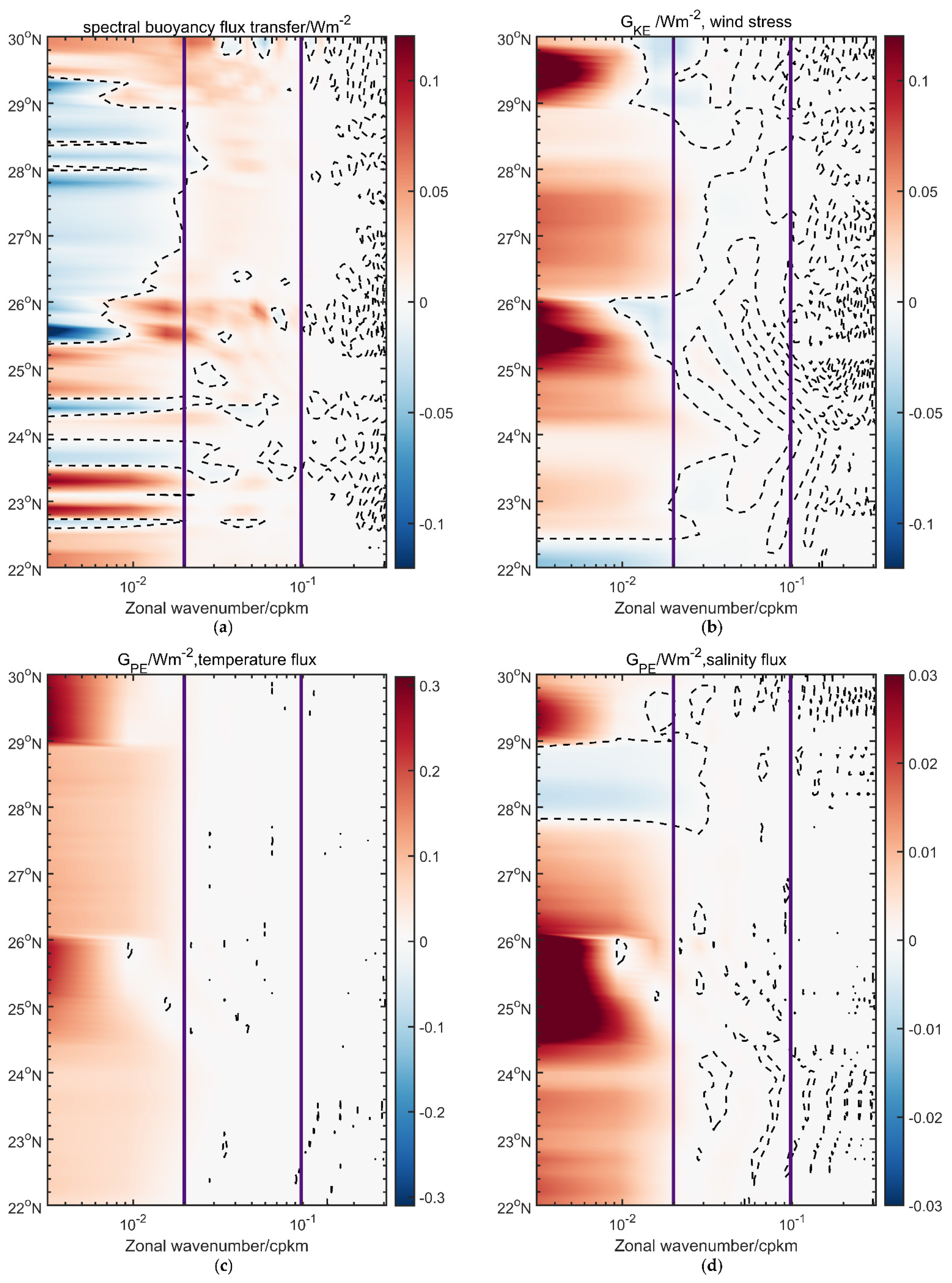
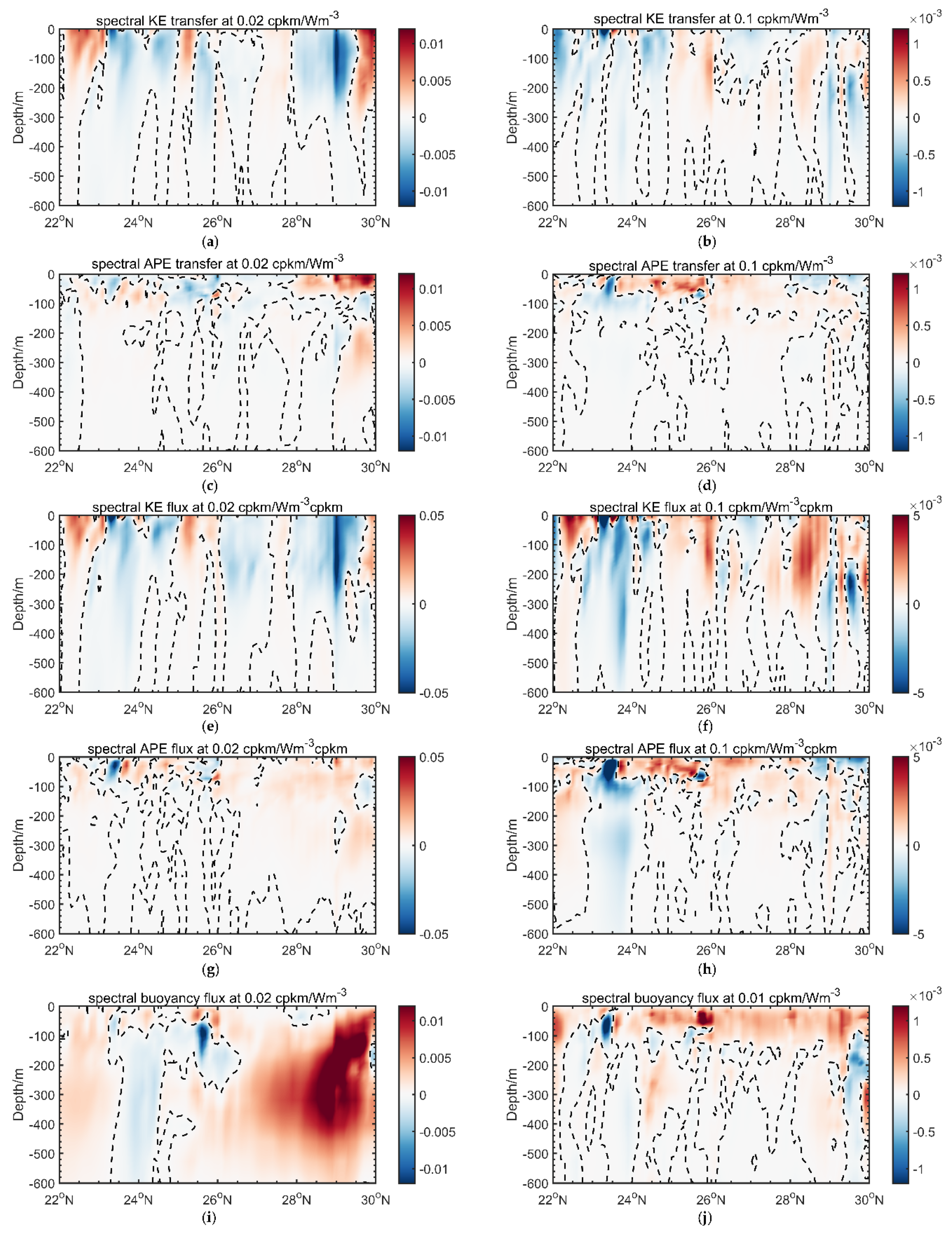
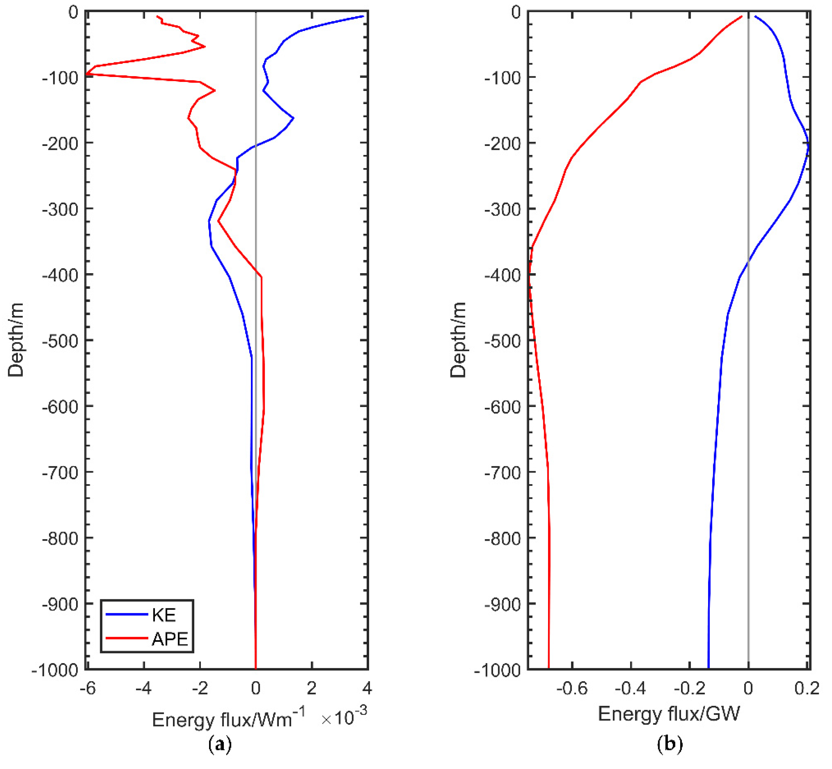
3.3. Generation of Energy Sources

First, we analyze the generation mechanism of sea surface energy sources. The spectral buoyancy flux, spectral KE generated by the wind stress and spectral APE generated by the temperature and salinity fluxes are calculated by using Equations (2), (3) and (7), respectively, to prove the above hypothesis, and their wavenumber–latitude distributions at the sea surface are shown in Figure 5. The spectral buoyancy flux at the sea surface integrated to 15 m depth, which is the density uniform layer depth (the distribution of temperature and salinity is basically uniform [34]), is presented in Figure 5a, in which positive values indicate an energy conversion from APE to KE. The main latitude ranges of the conversion from APE to KE are approximately 22°–23.6° N, 23.8°–24.2° N, 24.6°–25.4° N and 29.4°–30° N at the large scale and approximately 22°–30° N at the mesoscale. Combined with the positions of the KE sources in Figure 3a, the overlapping latitude ranges are mainly 23.2°–23.6° N and 23.8°–24.2° N for the large scale and 23.2°–25° N and 26°–30° N for the mesoscale. These overlapping regions indicate that the KE sources and the conversion from APE to KE caused by buoyancy flux exist simultaneously and account for most of the KE source locations, especially at the mesoscale. Therefore, buoyancy flux is a very important generation mechanism for KE sources, especially at the mesoscale. External forces such as wind stresses may also be important for KE source generation within latitude ranges without coincidence. Figure 5b shows that the spectral KE caused by wind stress takes a positive value at the locations of KE sources. The wind–generated power is passed to the ocean beneath via the shear-induced stress and via pressure [35], and part of the wind energy is converted to APE excited geostrophic eddies through baroclinic instability, which is converted to KE [36]. There is no doubt that wind stress is the main generation mechanism for KE sources at the sea surface, especially at a large scale. However, the spectral power input is almost negative in partial latitude ranges, meaning that the direction of the Kuroshio velocity component is opposite to that of the wind stress component; this is due to the East Asian monsoon, the path of which is oriented at an angle to the Kuroshio in the study region. As described in Wunsch [37], subtropical gyres are regions where the atmosphere operates similar to a brake on ocean circulation. However, at the mesoscale, it appears primarily as an energy sink because of a physical process called eddy killing (caused by a negative eddy wind work), which reduces the eddy–mean flow interaction (both forward and inverse cascade) [23]. Therefore, the KE cycle is a process in which the wind stress causes the generation of a KE source on one scale. To achieve a statistically stable state of spectral KE, KE will be redistributed to other scales, which nearly results in an inverse KE cascade. As discussed in Renault et al. [23], the role of fine–scale ocean–atmosphere coupling modifies the usual concept of wind-driven currents: wind is not simply a large–scale energy source that initiates a turbulent cascade; it also interacts at a fine scale and directly affects the entire oceanic spectrum.
A negative spectral buoyancy flux indicates energy conversion from KE to APE. Combined with the positions of the APE sources in Figure 4a, most latitude ranges are coincident at the large scale. This means that large-scale APE sources originate primarily from the conversion of KE to APE, whereas the APE sources in other locations are generated by external forces such as temperature and salinity fluxes. Temperature and salinity differences cause density differences, which arouse buoyancy contrasts that then cause the ocean to move, creating APE [15]. Figure 5c shows the spectral APE caused by the temperature flux; the temperature flux value is of the same order as the spectral buoyancy flux value, suggesting that the former plays an equally important role as the latter. The positive values over the whole latitude range indicate the generation of an APE source. We likewise conclude that the salinity flux shown in Figure 5d also plays a role in generating APE sources. Therefore, the APE cycle can be summarized as follows: the spectral buoyancy flux, temperature flux and salinity flux cause the generation of a large-scale APE source, and to make the spectral APE reach a steady state, an inverse or forward APE cascade will occur. At the mesoscale, the APE source will be generated by the temperature and salinity fluxes, eventually nearly resulting in an inverse APE cascade. In general, the APE source generation mechanism is mainly density differences at the sea surface.
Second, we analyze the generation mechanism of energy sources beneath the sea surface by discussing their vertical distribution. In the preceding section, 0.02 cpkm (a wavelength of approximately 314 km) and 0.1 cpkm (a wavelength of approximately 63 km) were taken as the boundary wavenumbers between the large scale and mesoscale and between the mesoscale and small scale, respectively. Therefore, we constructed vertical sections of the spectral energy transfer and spectral energy flux along these two wavenumbers, as shown in Figure 6a–h. Numerically, the spectral energy transfer is an order of magnitude higher at 0.02 cpkm than at approximately 0.1 cpkm. The transfer values gradually decrease with depth and approach zero. Figure 6a,b denote the spectral KE transfer at 0.02 cpkm and 0.1 cpkm, respectively. When the vertical section is along 0.02 cpkm, the extremum of spectral KE transfer is situated near 29° Nand can extend to 300 m. However, when the vertical section is along 0.1 cpkm, the extremum is near 23° N and extends to only 40 m. In addition, the higher absolute value of spectral KE transfer is located mainly above 400 m depth, and most of the values were originally negative. In other words, the KE sources exist mainly above a depth of 400 m. Combined with Figure 6e,f, the negative spectral KE transfer almost overlaps with the position of the negative spectral KE flux, indicating that the KE source corresponds to an inverse KE cascade beneath the sea surface. Figure 6c,d show that the extrema of the spectral APE transfer above a depth of 100 m are concentrated mainly within the range of 23°–26° N, whereas the negative spectral APE transfer (APE source) is distributed mainly above 200 m depth. In other words, the APE sources are distributed mainly within depths of 200 m, which is obviously shallower than the depth reached by the vertical distribution of KE sources, which may be related to the mixing layer. Combined with Figure 6g,h, the position of the negative spectral APE transfer is almost the same as that of the negative spectral flux. This means that the APE source also corresponds to the inverse APE cascade beneath the sea surface. Furthermore, the spectral APE transfer, which is partially positive, is located mainly above 400 m depth and is precisely opposite in phase to the distribution of spectral KE transfer. This may be caused by the spectral transfer properties of KE and APE, as shown in Figure 6i,j. The positive spectral buoyancy fluxes almost coincide with the positions of the KE sources, while the negative values almost coincide with the positions of the APE sources, suggesting that the buoyancy flux is the generation mechanism of energy sources beneath the sea surface.

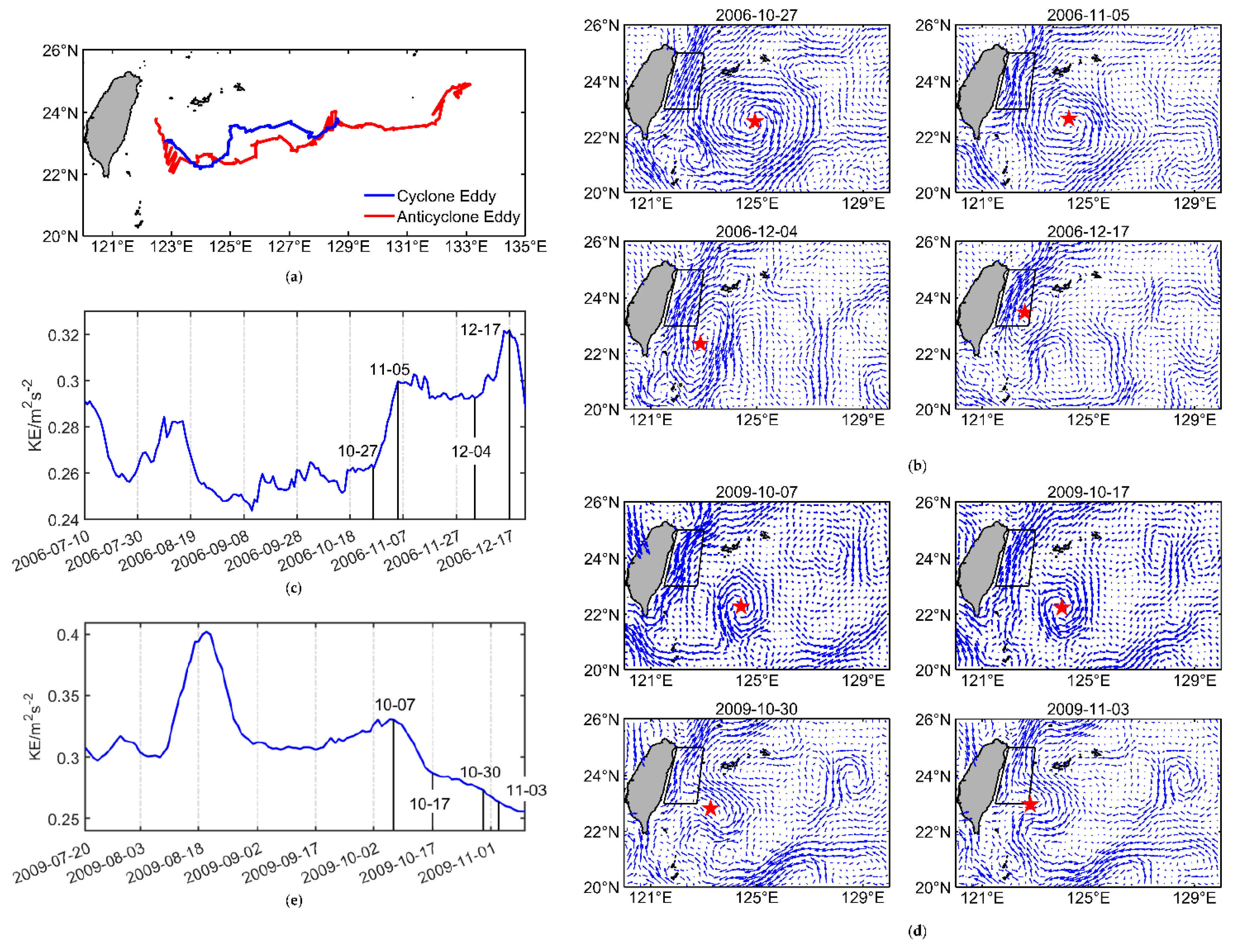
3.4. Marine Phenomena Associated with the Conversions of Energy

In this section, we take the energy conversion of the westward eddy on the east side of the Kuroshio east of Taiwan as an example to explain the generation of energy sources in the ocean, which also can be regarded as the phenomenon verification of LEC. Analysis by Qin et al. [30] led them to conclude that the increase in Kuroshio transport could enhance the instability of the flow by increasing shear strength to create more eddies, and the advection by the Kuroshio could produce more eddies than wind stress curl and topography; Liu et al. [9] found that eddies distributed across Kuroshio are generated by the horizontal velocity shear of the Kuroshio when it flows northeastward along the shelf break in East China Sea, and both the horizontal shear and vertical buoyancy flux are important energy sources for eddy generation. These processes involve the conversion of KE from large-scale to mesoscale, that is, the forward cascade of KE. In addition, the frontal eddy with the cold core as shown in Figure A1 around the shelf edge corresponded to the upwelling of cold slope water [38]. Gula et al. [39] used a very high–resolution model to simulate the Gulf Stream frontal eddy, and found that the sharp front between the frontal eddy and the stream is instantaneously composed of multiple sub–mesoscale fronts appearing as elongated vorticity filaments on the stream interior edge of the eddy. The same sub–mesoscale structure may exist in Kuroshio front vortexes, which requires further work. If true, the vigorous sub-mesoscale frontal instabilities can lead to secondary frontogenesis events, sub-mesoscale vortices and excitation of even smaller–scale flows, and the sub-mesoscale process efficiently releases APE to KE associated with baroclinic instability [40]. The above processes include the generation mechanism of KE sources.
Beyond that, there is also the energy transfer caused by the interaction of the Kuroshio and the westward moving eddies born in the north Pacific. The altimeter data were used to detect eddies in the north Pacific by using the Okubo–Weiss method [41,42]. The correlation distance was used to calculate the correlation of two different eddies [43] in order to track the eddy. Figure 7a shows the trajectories of an anticyclonic and a cyclonic eddy. The anticyclonic eddy was born in the north Pacific on 10 July 2006, and died in the Kuroshio east of Taiwan on 23 December 2006. The cyclonic eddy was born in the north Pacific on 20 July 2009, and died in the Kuroshio east of Taiwan on 10 November 2009. Figure 7b displays the last three months of the anticyclonic eddy’s life cycle. At this time, the eddy had moved to the Kuroshio region. We chose the region where the eddy finally disappeared as the study area and calculate the geographical average KE using AVISO data of this region. The time series of KE in the life cycle of the anticyclonic eddy is shown in Figure 7d. The KE was about 26.25 × 10⁻² m2s−2 on October 27, then suddenly increased to a maximum of about 29.98 × 10⁻² m2s−2 on November 5. The eddy had a circular shape and its edge entered the Kuroshio. It continued traveling west until November 5, when the eddy entered the Kuroshio region, causing an increase in KE over the study region. The KE fluctuated around this maximum, but on 4 December, it suddenly increased again and reached a maximum of 32.18 × 10⁻² m2s−2 on 17 December. On 4 December, the eddy’s shape changed into an ellipse with its long axis trending northeast and its short axis trending northwest. From 4 December to 17 December, the eddy core gradually approached the Kuroshio. As reported in Kuo and Chern [7], an anticyclonic eddy can obtain energy from the mean flow during the eddy–WBC interaction when one of the major axes trends NNE. The long axis of the eddy kept getting longer and the short axis kept getting shorter until 23 December, when it almost merged into the Kuroshio. This occurred because the eddy still decayed from losing its water and friction dissipation during the eddy–WBC interaction period [7]. The KE on 23 December was higher than on 27 October. In other words, the KE when the anticyclonic eddy died was higher than the KE when the eddy had just entered the Kuroshio. This shows that an anticyclonic eddy can enhance the Kuroshio.
Figure 7d shows the cyclonic eddy extinction process over Kuroshio. We chose the same region as that selected for the analysis of the anticyclonic eddy, and calculated the geographical average KE. The time series of KE in the anticyclonic eddy’s life cycle is shown in Figure 7e. The KE was about 33.04 × 10⁻² m2s−2 on 7 October and decreased to 28.68 × 10⁻² m2s−2 on 17 October, then the KE decreased at a slower rate. From Figure 7d, the cyclonic eddy has not reached the Kuroshio region during this period. The KE was about 27.30 × 10⁻² m2s−2 on 30 October, then it decreased at a faster rate and dropped to 26.37 × 10⁻² m2s−2 on 3 November. The cyclonic eddy entered the Kuroshio region on 30 October, and gradually became an ellipse with long axis trending northwest and short axis trending northeast. As per Kuo and Chern [7], during the eddy–WBC interaction, the major axis of a cyclonic eddy was aligning in a NW direction, and the cyclonic eddy can lose its energy to the mean flow. On 3 November, the long axis of the cyclonic eddy has shortened with its left velocity approaching zero. Then, the velocity on the right side of the cyclonic eddy gradually coincided with the Kuroshio. The KE on 10 November was lower than on 30 October. In other words, the KE when the cyclonic eddy died was lower than the KE when the eddy had just entered the Kuroshio. This shows that a cyclonic eddy can weaken the Kuroshio.

4. Discussion

Based on the above discussion, the accurate distribution of energy sources was obtained, and it was concluded that the wind stress and density differences contribute significantly to KE and APE source generation, respectively, at the sea surface, but undersurface, the density differences contribute significantly to energy source generation. To deepen the understanding of the energy source and sink, energy flux is introduced here. Traditionally, energy flux is defined as the rate of transfer of energy through a unit area. Here, we defined the energy flux as
ϕ = s v θ E d s
where v θ = v cos θ u sin θ is the velocity in the normal direction of the plane, θ is the inclination in the north–south direction and E is KE or APE. The negative flux indicates the outflow of energy, that is, the energy produced in the closed area is greater than the energy dissipated (energy source); the positive flux indicates the inflow of energy, that is, the energy produced in the closed area is less than the energy dissipated (energy sink).
The long-term mean energy fluxes in the large–scale energy source and sink regions are calculated as shown in Table 1. The KE flux integrated to 100 m depth in the source region is −4.57 GW and in the sink region is 4.70 GW, and in the total area (red box region in Figure 1) is 0.13 GW. The KE flux integrated to 600 m depth in the source region is −8.56 GW and in the sink region is 8.46 GW, and in the total area is −0.10 GW. The signs of the KE flux conform to the energy source and sink in Section 3. The sign of the KE flux over the total area changes from positive to negative, that is, the KE changes from inflow to outflow (sink to source). This may be because within 100 m to 600 m depth, the spectral buoyancy flux is positive (conversion from APE to KE) for large–scale, with KE generation greater than dissipation. The APE flux integrated to 100 m depth in the source region is −0.34 GW and in the sink region is −0.02 GW, and in the total area is −0.36 GW. The APE flux integrated to 600 m depth in the source region is −0.66 GW and in the sink region is −0.04 GW, and in the total area is −0.70 GW. The sign of APE over the sink region does not match because the regions are divided according to the large–scale source and sink, but the total velocity and density used to calculate the APE flux and the large–scale APE sink regions are represented as mesoscale APE sources. The total area showed an APE outflow, and the APE may be mainly generated from temperature and salinity fluxes, as shown in Figure 5c,d.
The curve of the energy flux with each layer is shown in Figure 8a. The KE flux is positive, but the APE flux is negative at the sea surface. The incoming KE has two directions: one is converted to APE outflow, and the other is converted to internal energy dissipation. The outflow of APE comes from two sources: air–sea interactions (temperature and salinity fluxes) and the conversion of KE to APE due to baroclinic instability. Above 100 m depth, the inflow KE decreased, and the outflow APE increased, indicating that the sea–air flux played an important role in APE generation in the closed area. Concluding from the Schematics of the energy budgets (see Figure 9, See Appendix B for explanation and calculation), the total APE generated by the sea–air flux is about 0.40 PW. At a depth of 100 m, the inflow of KE decreased and even flowed out gradually (about 200 m depth), while the outflow of APE decreased and even flowed in gradually (about 400 m depth), indicating that more APE was converted to KE due to buoyancy flux. Then, for the whole region, the energy flux of the integral curve is obtained by integrating each layer, as shown in Figure 8b. The KE flux is positive, and the APE is negative (KE inflow and APE outflow) down to 380 m depth. Then, the KE flux becomes negative (KE outflow), and the APE reaches a minimum at 400 m depth. Eventually, they leveled off (because of the terrain). Combining Figure 8a,b could be a process like this: first, the APE produced by temperature and salinity fluxes and converted by KE flowing in from outside flows out of the closed area. The APE outflow accumulates to its maximum when the depth reaches 400 m. Subsequently, the KE turns to outflow, the outflow of KE increases and APE decreases. As shown in Figure 9b, the whole area shows the conversion from KE to APE whose rate is about 1.16 PW. What causes enough KE to ensure the negative KE flux (the KE flow out of the closed area) and the conversion from KE to APE in the closed area, and makes KE reservoirs approximately 6.81 PJ at 400 m depth? That needs further proof.

5. Conclusions

In this paper, we found that in the wavenumber range of approximately 0.02 to 0.1 cpkm (wavelengths of approximately 314 to 63 km), the slope of the one–dimensional spectral energy density varies between −5/3 and −3. This illustrates that an inverse energy cascade occurs over the Kuroshio. In other words, energy is redistributed, which can be represented as a spectral energy transfer, and this spectral energy transfer reflects the power source and sink under steady-state conditions. Additionally, the source is defined as a forced term greater than the dissipative term, and the average Rhines scale in the study region is approximately 1217 km, which means that energy sources occur at scales smaller than this value. The wavenumber–latitude distribution of spectral energy transfer was used to determine the locations of energy sources at the sea surface. The KE sources are mainly within 23.2°–25.6° N and 28°–29° N at less than 0.02 cpkm and within 23.2°–25° N and 26°–30° N at 0.02–0.1 cpkm; the APE sources are mainly within 22°–28° N and 28.6°–30° N at less than 0.02 cpkm and within 22.6°–24.6° N, 25.4°–28° N and 29.2°–30° N at 0.02–0.1 cpkm. Some of the locations of the KE and APE sources overlap, especially at the large scales. This suggests that large-scale energy sources in overlapping regions are caused by external forces. Then, we integrated the spectral energy transfer to obtain the spectral energy flux. As a result, at the same location and scale, most of the energy sources correspond to a zonal inverse energy cascade, although some forward cascades occur at the large scale, especially for the APE sources.
Next, the generation mechanisms responsible for the energy sources were analyzed. From a mathematical perspective, the buoyancy flux and atmospheric forcing may influence the distribution of energy sources. Hence, we calculated the spectral buoyancy flux and the spectral energies caused by the wind stress, temperature flux and salinity flux at the sea surface. Wind stress and buoyant flux together are responsible for the KE sources; between them, wind stress plays a major role. The KE cycle is a process in which the wind stress causes the generation of a KE source on one scale. Hence, to achieve a statistically steady state of spectral KE, KE will be redistributed to other scales, nearly resulting in an inverse KE cascade. Temperature and salinity fluxes and buoyancy flux play almost equally important roles in the generation of APE sources. That is, the mechanism of APE production is mainly density differences. The APE cycle is a process in which density differences generate APE sources. To achieve steady-state APE, both inverse and forward large-scale APE cascades and an inverse mesoscale APE cascade will occur. Subsequently, we constructed vertical sections of the spectral energy transfer and spectral energy flux along 0.02 and 0.1 cpkm. Larger absolute values of spectral energy transfer are located mainly above 400 m depth. Furthermore, the spectral KE transfer distributed above 400 m depth is basically opposite in phase to the spectral APE transfer. Combined with the vertical profile of the spectral buoyancy flux, the generation mechanism of an energy source is the buoyancy flux, and the energy source corresponds to an inverse energy cascade beneath the sea surface. Hence, the energy cycle beneath the sea surface is a process in which the buoyancy flux generates the energy source. To achieve a statistically steady state of spectral energy, the energy is redistributed to other scales, nearly resulting in an inverse energy cascade. Oceanic phenomena such as generation of eddies, eddy–Kuroshio interaction and frontal eddies reflect the energy cascade and energy conversion.
Finally, we calculate the energy flux to prove the energy source and sink. The sign of the KE flux corresponds well to the KE source and sink. However, the sign of the APE flux cannot correspond to the APE sink, and the reason for this phenomenon needs further proof. Energy flux integral curves along depth are obtained, which may be a process. When the integrated depth is lower than 380 m, the KE inflow is converted to the APE flowing out of the closed area. The APE outflow accumulates to its maximum when the integrated depth reaches 400 m. In survey region, the KE changes from sink to source and APE is represented as source with the changes of depth.

Author Contributions

All the authors have made significant contributions to this study. Conceptualization, Y.H. and R.W.; methodology, R.W. and Z.L.; data analysis, R.W.; writing—original draft preparation, R.W.; writing—review and editing, R.W., Y.H. and Z.L.; supervision, Y.H.; funding acquisition, Y.H. and Z.L. All authors have read and agreed to the published version of the manuscript.

Funding

The research was funded by the National Natural Science Foundation of China (Grants 41630967 and 41776020).

Institutional Review Board Statement

Not applicable.

Informed Consent Statement

Not applicable.

Data Availability Statement

Data available in a publicly accessible repository that does not issue DOIs. The OFES data were obtained from the Asia-Pacific Data-Research Center (APDRC, http://apdrc.soest.hawaii.edu/data). The geographic velocity and sea level anomaly data were obtained from the Copernicus Marine Environment Monitoring Service (CMEMS, http://marine.copernicus.eu/). Copernicus Climate Change Service (C3S) (2017): ERA5: Fifth-generation ECMWF atmospheric reanalysis of the global climate. Copernicus Climate Change Service Climate Data Store (CDS), 22 September 2020. https://cds.climate.copernicus.eu/cdsapp#!/home.

Acknowledgments

The OFES data were obtained from the Asia-Pacific Data-Research Center (APDRC, http://apdrc.soest.hawaii.edu/data). The geographic velocity and sea level anomaly data were obtained from the Copernicus Marine Environment Monitoring Service (CMEMS, http://marine.copernicus.eu/). Copernicus Climate Change Service (C3S) (2017): ERA5: Fifth-generation ECMWF atmospheric reanalysis of the global climate. Copernicus Climate Change Service Climate Data Store (CDS), 22/09/2020. https://cds.climate.copernicus.eu/cdsapp#!/home. This research was supported by the National Natural Science Foundation of China (through the grants of No. 41630967 and No. 41776020). The M-Map toolbox [44] of MATLAB was used to create the graphics. The Gibbs Seawater (GSW) oceanographic toolbox [45] of MATLAB was used to calculate the density of seawater. The authors are grateful for the above data, financial and technical support.

Conflicts of Interest

The authors declare no conflict of interest.

Appendix A. Evolution Equation for Spectral Energy

The appendix shows the derivation of the evolution equation for spectral energy. Under static equilibrium and Boussinesq approximation, the N-S equation, transport equation and continuity equation of wind stress and sea–air flux are considered as
u t + u u x + v u y f v = 1 ρ 0 p x + 1 ρ 0 τ x z + F r x
v t + u v x + v v y + f u = 1 ρ 0 p y + 1 ρ 0 τ y z + F r y
ρ a t + u ρ a x + v ρ a y = ρ 0 N 2 g w + α 0 J z + β 0 G z
u x + v y + w z = 0
and   p z = ρ a g
where ρ 0 = 1025   kg   m 3 is the constant reference density; τ = ( τ x , τ y ) is the vertical flux of horizontal momentum vector [46]; the total density is given by ρ ( x , y , z , t ) = ρ r ( z ) + ρ a ( x , y , z , t ) and ρ r and ρ a are the reference and perturbation densities, respectively; N 2 = ( g / ρ 0 ) d ρ r / d z , where N is the buoyancy frequency; α 0 = ( ρ T ) p , S and β 0 = ( ρ S ) ρ , T denote the thermal expansion coefficient and saline contraction coefficient, respectively; J and G are the vertical eddy fluxes of temperature and salt due to air–sea exchange [46].
Frist, the Fourier transform of Equations (A1) and (A2) are multiplied by ρ 0 u ^ and ρ 0 v ^ and then added together as Qiu et al. [14] is done. The evolution equation for spectral KE is
K E t = ρ 0 [ u ^ ( u u x + v u y ) + v ^ ( u v x + v v y ) ] g ( w ^ ρ ^ a ) + ( u ^ τ x z + v ^ τ y z ) D K E
where the spectral KE is K E = ρ 0 ( u ^ u ^ + v ^ v ^ ) / 2 . Then, the Fourier transform of Equation (A3) is multiplied by g 2 ρ 0 N 2 ρ ^ a , the evolution equation for spectral APE is
A P E t = g 2 ρ 0 N 2 [ ρ ^ a ( u ρ a x + v ρ a y ) ] + g ( ρ ^ a w ^ ) + g 2 ρ 0 N 2 ( α 0 ρ ^ a J z + β 0 ρ ^ a G z ) D P E
The spectral APE is defined as A P E = g 2 2 ρ 0 N 2 ρ ^ a ρ ^ a , where the curly brackets with carets indicate the discrete Fourier transform, the asterisk indicates the complex conjugate, and takes the real part of an imaginary number. Some transfer terms, generate terms and friction terms have been obtained, which are the spectral KE transfer terms
T K E = ρ 0 [ u ^ ( u u x + v u y ) + v ^ ( u v x + v v y ) ]
the spectral density variance (APE) transfer term
T P E = g 2 ρ 0 N 2 [ ρ ^ a ( u ρ a x + v ρ a y ) ]
the spectral buoyancy flux
B = g ( w ^ ρ ^ a ) = g ( ρ ^ a w ^ )
the spectral KE generation term
G K E = ( u ^ τ x z + v ^ τ y z )
caused by wind stress, this term can be expressed as G K E , s = ( u ^ τ ^ x , s + v ^ τ ^ y , s ) on the sea surface; the spectral density variance (APE) generation term
G P E = g 2 ρ 0 N 2 ( α 0 ρ ^ a J z + β 0 ρ ^ a G z )
caused by the temperature and salinity fluxes, this term can be expressed as G P E , s = ( α 0 , s ρ ^ a J ^ s + β 0 , s ρ ^ a G ^ s ) on the sea surface. J s = H ρ S c p and G s = S ¯ ( E P ) are the temperature and salinity fluxes at the sea surface, respectively, where c p = 4000   J   kg - 1 K - 1 is the specific heat capacity of seawater, H is the total heat flux at the sea surface, S ¯ is the time-mean salinity in the uppermost model layer, and E and P are the evaporation and precipitation rates, respectively [15,46].

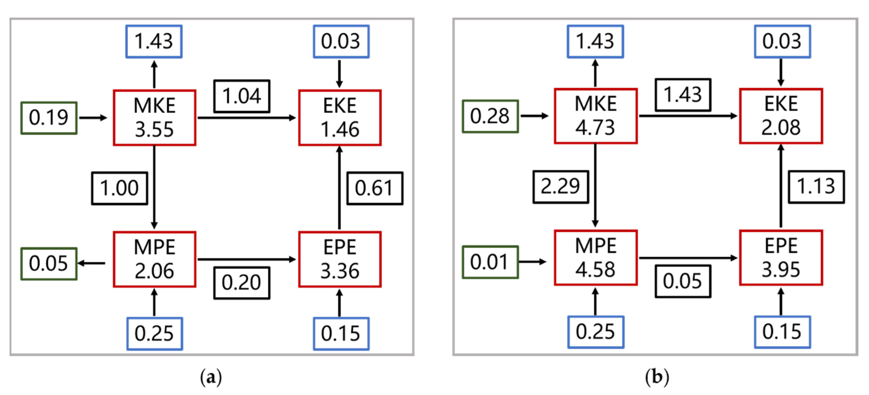
Appendix B. Lorentz Energy Cycle

The LEC describes the steady-state balance among the mean kinetic energy (MKE), eddy kinetic energy (EKE), mean available potential energy (MPE) and eddy available potential energy (EPE) [46]. These four energy reservoirs are obtained by using the Reynolds decomposition technique from the field of fluid dynamics. This method has been used in many other studies [11,18,46,47,48] to calculate the energy budgets of coupled eddy–mean flow systems. Then, the four energy reservoirs are defined as
M K E = ρ 0 ( u ¯ 2 + v ¯ 2 ) / 2
E K E = ρ 0 ( u 2 + v 2 ) ¯ / 2
M P E = g 2 ρ ¯ a 2 / 2 ρ 0 N 2
and   E P E = g 2 ρ a 2 ¯ / 2 ρ 0 N 2 .  
where the ρ a = ( ρ ρ r ) ( ρ ρ r ) ¯ = ρ ρ ¯ = ρ . Energy conversions are obtained from Equations (A1)–(A5) transformation. The barotropic MKE→EKE conversion through eddy momentum fluxes and Reynolds stresses between mean and perturbed flows is:
B T C = ρ 0 ( u u ¯ u ¯ + v u ¯ v ¯ )
where u = ( u , v ) is the velocity vector and the prime symbol denotes the deviation from the time mean. The equation for baroclinic MPE→EPE conversion through the horizontal eddy density flux is:
B C C = g 2 ρ 0 N 2 u ρ a ¯ ρ ¯ a
where positive (negative) values of the barotropic conversion (BTC) and baroclinic conversion (BCC) rate terms indicate mean-to-eddy (eddy-to-mean) energy conversion. The gain rate of KE from APE through the mean buoyancy flux is:
V M D F = g ρ ¯ a w ¯
The gain rate of KE from APE through the vertical eddy density flux is:
V E D F = g ρ a w ¯
Positive (negative) values of these terms indicate a PE to KE (KE to PE) conversion. The nonlocal EKE → MKE conversion is
N L K M = ρ 0 [ ( u u u ¯ ) ¯ + ( u v u ¯ ) ¯ ]
and the nonlocal EPE → MPE conversion is
N L P E = g 2 ρ 0 N 2 ( u ρ a ρ ¯ a ) ¯
At the sea surface, the rates of generation of MKE and EKE are:
G M K E = τ ¯ x , s u ¯ + τ ¯ y , s v ¯
and
G E K E = τ x , s u ¯ + τ y , s v ¯
which are related to wind stress. The rates of generation of MPE and EPE are:
G M P E = g 2 α 0 ρ 0 N 2 J ¯ s ρ ¯ a + g 2 β 0 ρ 0 N 2 G ¯ s ρ ¯ a
and
G E P E = g 2 α 0 ρ 0 N 2 J s ρ a ¯ + g 2 β 0 ρ 0 N 2 G s ρ a ¯
which are related to the temperature and salinity fluxes.

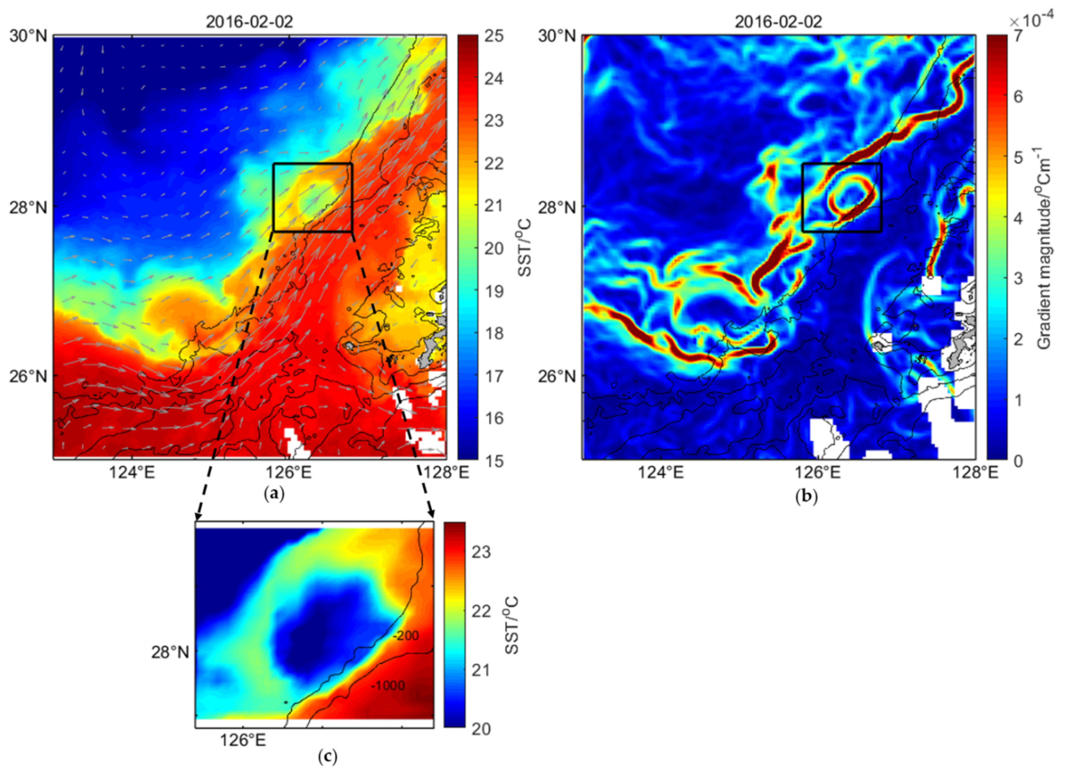
Appendix C. The Frontal Eddy

There are fronts and frontal eddies around Kuroshio, and the energy conversion caused by them is discussed with the example of 2 February 2016 in Figure A1. Figure A1a shows the distribution of SST provided by MODIS on 2 February 2016. Thermal fronts lay between Kuroshio and the East China Sea, and a distinct frontal eddy existed nearby 28 °N, 126 °N adjacent to the 200 m isobath. The thermal fronts create sharp horizontal gradients of SST, and we used gradient method for front detection. Median filter was applied to the SST image to suppress noise before front detection. The gradient vectors Gx and Gy are calculated by the Sobel operator consisting of two convolution masks: GX= [−1 0 +1; −2 0 +2; −1 0 +1]; GY= [+1 +2 +1; 0 0 0; −1 −2 −1]. If A is the original image, G x = G X A and G y = G Y A , where is the convolution sign [49]. The gradient magnitude G M = G x 2 + G y 2 is shown in Figure A1. The position of thermal fronts and the frontal eddy can be obtained obviously. The frontal eddy was on the Kuroshio side of the front. Figure A1 shows the detailed structure of the frontal eddy with an appropriate color bar.
Figure A1. Sea surface phenomenon over Kuroshio in the East China Sea on 2 February 2016. (a) Distribution of SST provided by MODIS data and velocity vector derived from AVISO data; (b) Distribution of SST gradient magnitude computed by Sobel operator; (c) Detail distribution of the frontal eddy. The gray arrows indicate the absolute geography velocity. The black boxes represent the frontal eddy. The black solid lines indicate the 200 m, 1000 m and 2000 m isobaths.
Jmse 09 00692 g0a1

References

  1. Hwang, C.; Wu, C.-R.; Kao, R. TOPEX/Poseidon observations of mesoscale eddies over the Subtropical Countercurrent: Kinematic characteristics of an anticyclonic eddy and a cyclonic eddy. J. Geophys. Res. Oceans 2004, 109, C08013. [Google Scholar] [CrossRef] [Green Version]
  2. Hsin, Y.C.; Wu, C.R.; Shaw, P.T. Spatial and temporal variations of the Kuroshio east of Taiwan, 1982–2005: A numerical study. J. Geophys. Res. Oceans 2008, 113, C04002. [Google Scholar] [CrossRef] [Green Version]
  3. Hsin, Y.C.; Qu, T.D.; Wu, C.R. Intra-seasonal variation of the Kuroshio southeast of Taiwan and its possible forcing mechanism. Ocean Dyn. 2010, 60, 1293–1306. [Google Scholar] [CrossRef]
  4. Hsin, Y.C.; Qiu, B.; Chiang, T.L.; Wu, C.R. Seasonal to interannual variations in the intensity and central position of the surface Kuroshio east of Taiwan. J. Geophys. Res. Oceans 2013, 118, 4305–4316. [Google Scholar] [CrossRef]
  5. Yin, Y.; Lin, X.; He, R.; Hou, Y. Impact of mesoscale eddies on Kuroshio intrusion variability northeast of Taiwan. J. Geophys. Res. Oceans 2017, 122, 3021–3040. [Google Scholar] [CrossRef]
  6. Ebuchi, N.; Hanawa, K. Trajectory of mesoscale eddies in the Kuroshio recirculation region. J. Oceanogr. 2001, 57, 471–480. [Google Scholar] [CrossRef]
  7. Kuo, Y.C.; Chern, C.S. Numerical study on the interactions between a mesoscale eddy and a western boundary current. J. Oceanogr. 2011, 67, 263–272. [Google Scholar] [CrossRef]
  8. Kamidaira, Y.; Uchiyama, Y.; Mitarai, S. Eddy-induced transport of the Kuroshio warm water around the Ryukyu Islands in the East China Sea. Cont. Shelf Res. 2017, 143, 206–218. [Google Scholar] [CrossRef]
  9. Liu, Y.; Dong, C.; Liu, X.; Dong, J. Antisymmetry of oceanic eddies across the Kuroshio over a shelfbreak. Sci. Rep. 2017, 7, 6761. [Google Scholar] [CrossRef] [PubMed] [Green Version]
  10. Yang, Y.; Liang, X.S. The intrinsic nonlinear multiscale interactions among the mean flow, low frequency variability and mesoscale eddies in the Kuroshio region. Sci. China Earth Sci. 2019, 62, 595–608. [Google Scholar] [CrossRef]
  11. Yan, X.; Kang, D.; Curchitser, E.N.; Pang, C. Energetics of Eddy–Mean Flow Interactions along the Western Boundary Currents in the North Pacific. J. Phys. Oceanogr. 2019, 49, 789–810. [Google Scholar] [CrossRef]
  12. Kraichnan, R.H. Inertial range in two-dimensional turbulence. Phys. Fluids 1967, 10, 1417–1423. [Google Scholar] [CrossRef] [Green Version]
  13. Scott, R.B.; Wang, F. Direct evidence of an oceanic inverse kinetic energy cascade from satellite altimetry. J. Phys. Oceanogr. 2005, 35, 1650–1666. [Google Scholar] [CrossRef]
  14. Qiu, B.; Scott, R.B.; Chen, S. Length Scales of Eddy Generation and Nonlinear Evolution of the Seasonally Modulated South Pacific Subtropical Countercurrent. J. Phys. Oceanogr. 2008, 38, 1515–1528. [Google Scholar] [CrossRef] [Green Version]
  15. Gill, A.E. Atmosphere-Ocean Dynamics; Academic Press: New York, NY, USA, 1982; p. 662. [Google Scholar]
  16. Ferrari, R.; Wunsch, C. Ocean Circulation Kinetic Energy: Reservoirs, Sources, and Sinks. Annu. Rev. Fluid Mech. 2009, 41, 253–282. [Google Scholar] [CrossRef] [Green Version]
  17. Wang, S.; Liu, Z.; Pang, C. Geographical distribution and anisotropy of the inverse kinetic energy cascade, and its role in the eddy equilibrium processes. J. Geophys. Res. Oceans 2015, 120, 4891–4906. [Google Scholar] [CrossRef]
  18. Kang, D.J.; Curchitser, E.N. Energetics of Eddy-Mean Flow Interactions in the Gulf Stream Region. J. Phys. Oceanogr. 2015, 45, 1103–1120. [Google Scholar] [CrossRef]
  19. Arbic, B.K.; Polzin, K.L.; Scott, R.B.; Richman, J.G.; Shriver, J.F. On Eddy Viscosity, Energy Cascades, and the Horizontal Resolution of Gridded Satellite Altimeter Products. J. Phys. Oceanogr. 2013, 43, 283–300. [Google Scholar] [CrossRef] [Green Version]
  20. Schlosser, F.; Eden, C. Diagnosing the energy cascade in a model of the North Atlantic. Geophys. Res. Lett. 2007, 34, L02604. [Google Scholar] [CrossRef] [Green Version]
  21. Scott, R.B.; Arbic, B.K. Spectral Energy Fluxes in Geostrophic Turbulence: Implications for Ocean Energetics. J. Phys. Oceanogr. 2007, 37, 673–688. [Google Scholar] [CrossRef]
  22. Capet, X.; Klein, P.; Hua, B.L.; Lapeyre, G.; Mcwilliams, J.C. Surface kinetic energy transfer in surface quasi-geostrophic flows. J. Fluid Mech. 2008, 604, 165–174. [Google Scholar] [CrossRef] [Green Version]
  23. Renault, L.; Marchesiello, P.; Masson, S.; McWilliams, J.C. Remarkable Control of Western Boundary Currents by Eddy Killing, a Mechanical Air-Sea Coupling Process. Geophys. Res. Lett. 2019, 46, 2743–2751. [Google Scholar] [CrossRef] [Green Version]
  24. Masumoto, Y.; Sasaki, H.; Kagimoto, T.; Komori, N.; Ishida, A.; Sasai, Y.; Miyama, T.; Motoi, T.; Mitsudera, H.; Takahashi, K. A fifty-year eddy-resolving simulation of the world ocean: Preliminary outcomes of OFES (OGCM for the Earth Simulator). J. Earth Simulator 2004, 1, 35–56. [Google Scholar]
  25. Sasaki, H.; Nonaka, M.; Masumoto, Y.; Sasai, Y.; Uehara, H.; Sakuma, H. An eddy-resolving hindcast simulation of the quasiglobal ocean from 1950 to 2003 on the Earth Simulator. In High Resolution Numerical Modelling of the Atmosphere and Ocean; Kevin, H., Wataru, O., Eds.; Springer: Berlin/Heidelberg, Germany, 2008; pp. 157–185. [Google Scholar] [CrossRef]
  26. Hersbach, H.; Bell, B.; Berrisford, P.; Hirahara, S.; Horányi, A.; Muñoz-Sabater, J.; Nicolas, J.; Peubey, C.; Radu, R.; Schepers, D.; et al. The ERA5 global reanalysis. Q. J. R. Meteorol. Soc. 2020, 146, 1999–2049. [Google Scholar] [CrossRef]
  27. Adrian, S.; Cornel, S.; Julien, N.; Bill, B.; Berrisford, P.; Rossana, D.; Johannes, F.; Leopold, H.; Sean, H.; Hans, H.; et al. Global Stratospheric Temperature Bias and Other Stratospheric Aspects of ERA5 and ERA5.1; European Centre for Medium Range Weather Forecasts: Reading, UK, 2020. [Google Scholar] [CrossRef]
  28. Large, W.G.; Pond, S. Open Ocean Momentum Flux Measurements in Moderate To Strong Winds. J. Phys. Oceanogr. 1981, 11, 324–336. [Google Scholar] [CrossRef] [Green Version]
  29. Trenberth, K.E.; Large, W.G.; Olson, J.G. The Mean Annual Cycle in Global Ocean Wind Stress. J. Phys. Oceanogr. 1990, 20, 1742–1760. [Google Scholar] [CrossRef] [Green Version]
  30. Qin, D.D.; Wang, J.H.; Liu, Y.; Dong, C.M. Eddy analysis in the Eastern China Sea using altimetry data. Front. Earth Sci. 2015, 9, 709–721. [Google Scholar] [CrossRef]
  31. Rhines, P.B. Waves and Turbulence on a Beta-Plane. J. Fluid Mech. 1975, 69, 417–443. [Google Scholar] [CrossRef] [Green Version]
  32. Sukoriansky, S.; Dikovskaya, N.; Galperin, B. On the Arrest of Inverse Energy Cascade and the Rhines Scale. J. Atmos. Sci. 2007, 64, 3312–3327. [Google Scholar] [CrossRef]
  33. Sérazin, G.; Penduff, T.; Barnier, B.; Molines, J.-M.; Arbic, B.K.; Müller, M.; Terray, L. Inverse Cascades of Kinetic Energy as a Source of Intrinsic Variability: A Global OGCM Study. J. Phys. Oceanogr. 2018, 48, 1385–1408. [Google Scholar] [CrossRef]
  34. An, Y.Z.; Zhang, R.; Wang, H.Z.; Chen, J.; Chen, Y.D. Study on calculation and spatio-temporal variations of global ocean mixed layer depth. Chin. J. Geophys. 2012, 55, 2249–2258. [Google Scholar]
  35. Von Storch, J.S.; Sasaki, H.; Marotzke, J. Wind-generated power input to the deep ocean: An estimate using a 1/10 degrees general circulation model. J. Phys. Oceanogr. 2007, 37, 657–672. [Google Scholar] [CrossRef]
  36. Cessi, P.; Young, W.R.; Polton, J.A. Control of large-scale heat transport by small-scale mixing. J. Phys. Oceanogr. 2006, 36, 1877–1894. [Google Scholar] [CrossRef] [Green Version]
  37. Wunsch, C. The work done by the wind on the oceanic general circulation. J. Phys. Oceanogr. 1998, 28, 2332–2340. [Google Scholar] [CrossRef]
  38. Yanagi, T.; Shimizu, T.; Lie, H.J. Detailed structure of the Kuroshio frontal eddy along the shelf edge of the East China Sea. Cont. Shelf. Res. 1998, 18, 1039–1056. [Google Scholar] [CrossRef]
  39. Gula, J.; Molemaker, M.J.; McWilliams, J.C. Submesoscale Dynamics of a Gulf Stream Frontal Eddy in the South Atlantic Bight. J. Phys. Oceanogr. 2016, 46, 305–325. [Google Scholar] [CrossRef]
  40. Capet, X.; Mcwilliams, J.C.; Molemaker, M.J.; Shchepetkin, A.F. Mesoscale to submesoscale transition in the California current system. Part II: Frontal processes. J. Phys. Oceanogr. 2008, 38, 44–64. [Google Scholar] [CrossRef] [Green Version]
  41. Okubo, A. Horizontal dispersion of floatable particles in the vicinity of velocity singularities such as convergences. Deep Sea Res. Oceanogr. Abstr. 1970, 17, 445–454. [Google Scholar] [CrossRef]
  42. Weiss, J. The dynamics of enstrophy transfer in two-dimensional hydrodynamics. Physica. D 1991, 48, 273–294. [Google Scholar] [CrossRef]
  43. Penven, P.; Echevin, V.; Pasapera, J.; Colas, F.; Tam, J. Average circulation, seasonal cycle, and mesoscale dynamics of the Peru Current System: A modeling approach. J. Geophys. Res. Oceans 2005, 110, C10021. [Google Scholar] [CrossRef]
  44. Pawlowicz, R. M_Map: A Mapping Package for MATLAB. 2018. Available online: www.eoas.ubc.ca/rich/map.html (accessed on 23 June 2021).
  45. McDougall, T.J.; Barker, P.M. Getting Started with TEOS-10 and the Gibbs Seawater (GSW) Oceanographic Toolbox. SCOR/IAPSO WG 2011, 127, 1–28. [Google Scholar]
  46. Von Storch, J.S.; Eden, C.; Fast, I.; Haak, H.; Hernandez-Deckers, D.; Maier-Reimer, E.; Marotzke, J.; Stammer, D. An Estimate of the Lorenz Energy Cycle for the World Ocean Based on the 1/10 degrees STORM/NCEP Simulation. J. Phys. Oceanogr. 2012, 42, 2185–2205. [Google Scholar] [CrossRef]
  47. Cronin, M.; Watts, D.R. Eddy–Mean Flow Interaction in the Gulf Stream at 68° W. Part I: Eddy Energetics. J. Phys. Oceanogr. 1996, 26, 2107–2131. [Google Scholar] [CrossRef] [Green Version]
  48. Chen, R.; Flierl, G.R.; Wunsch, C. A Description of Local and Nonlocal Eddy-Mean Flow Interaction in a Global Eddy-Permitting State Estimate. J. Phys. Oceanogr. 2014, 44, 2336–2352. [Google Scholar] [CrossRef] [Green Version]
  49. Belkin, I.M.; O’Reilly, J.E. An algorithm for oceanic front detection in chlorophyll and SST satellite imagery. J. Mar. Syst. 2009, 78, 319–326. [Google Scholar] [CrossRef]
Figure 1. Geographical distribution of the sea surface velocity based on the OFES data. The red box represents the Kuroshio of Taiwan Island and the East China Sea. The gray solid lines indicate the 200 m, 1000 m and 2000 m isobaths. The white solid lines represent a constant velocity of 0.25 m s−1.
Jmse 09 00692 g001
Figure 2. One–dimensional spectral energy density at the sea surface. (a) Spectral KE density calculated by the OFES data and AVISO data; (b) spectral APE density calculated by the OFES data. The blue and red lines represent OFES data and AVISO data. The shading represents the 95% confidence interval. The black dotted and solid lines correspond to slopes of −5/3 and −3, respectively. The gray lines correspond to wavenumbers of approximately 0.02 cpkm and 0.1 cpkm (wavelengths of approximately 314 km and 63 km, respectively). The abbreviation cpkm signifies cycles per kilometer.
Jmse 09 00692 g002
Figure 3. Wavenumber–latitude distribution of the sea surface spectral KE transfer and spectral KE flux diagnosed from Equations (1) and (5) over Kuroshio. (a) Spectral KE transfer; (b) spectral KE flux. The black dotted lines denote the spectral KE transfer and spectral KE flux equal to zero. The purple lines correspond to wavenumbers of approximately 0.02 cpkm and 0.1 cpkm (wavelengths of approximately 314 km and 63 km, respectively).
Jmse 09 00692 g003
Figure 4. Wavenumber–latitude distributions of the sea surface spectral APE transfer and spectral APE flux diagnosed from Equations (6) and (9), respectively, over the Kuroshio. (a) Spectral APE transfer; (b) spectral APE flux. The spectral density variance transfer and spectral density variance flux are zero along the black dotted lines. The purple lines correspond to wavenumbers of approximately 0.02 cpkm and 0.1 cpkm (wavelengths of approximately 314 km and 63 km, respectively).
Jmse 09 00692 g004
Figure 5. Generation of energy sources calculated by Equations (2), (3) and (7) at the sea surface. (a) Spectral buoyancy flux (integrated to 15 m depth); (b) spectral KE caused by wind stress; (c) spectral APE caused by the temperature flux; (d) spectral APE caused by salinity flux. The black dotted lines indicate that the terms are equal to zero. The purple lines correspond to wavenumbers of approximately 0.02 cpkm and 0.1 cpkm (wavelengths of approximately 314 km and 63 km, respectively).
Jmse 09 00692 g005
Figure 6. Vertical sections of the spectral energy transfer, spectral energy flux and spectral buoyancy flux. (a) Spectral KE transfer at 0.02 cpkm; (b) spectral KE transfer at 0.1 cpkm; (c) spectral APE transfer at 0.02 cpkm; (d) spectral APE transfer at 0.1 cpkm; (e) spectral KE flux at 0.02 cpkm; (f) spectral KE flux at 0.1 cpkm; (g) spectral APE flux at 0.02 cpkm; (h) spectral APE flux at 0.1 cpkm; (i) spectral buoyancy flux at 0.02 cpkm; (j) spectral buoyancy flux at 0.1 cpkm. The black dotted lines indicate that the terms are equal to zero.
Jmse 09 00692 g006
Figure 7. An anticyclonic and a cyclonic eddy: both were born in the north Pacific and died with Kuroshio in the east of Taiwan. (a) The trajectories of the anticyclonic eddy and the cyclonic eddy; (b) Distribution of absolute geostrophic velocity vector derived from AVISO data during anticyclonic eddy extinction; (c) Time series of KE of the selected region, from the time of the anticyclonic eddy generation to the time of the eddy death; (d) Distribution of absolute geostrophic velocity vector derived from AVISO data during cyclonic eddy extinction; (e) Time series of KE of the selected region, from the time of the cyclonic eddy generation to the time of the eddy death. The red star indicates the eddy core. The black solid rectangle box represents the selected area.
Jmse 09 00692 g007
Figure 8. The curve of the energy flux along the depth over the survey region. (a) The energy flux varies with depth; (b) the integral curve of the energy flux with depth. The blue line is the KE flux; the red line is the APE flux.
Jmse 09 00692 g008
Figure 9. Schematics of the energy budgets over the survey region. (a) The energy budgets integrated to 200 m depth; (b) the energy budgets integrated to 400 m depth. The red boxes are energy reservoirs (MKE: mean kinetic energy; EKE: eddy kinetic energy; MPE: mean available potential energy; EPE: eddy available potential energy) with units of PJ (PJ = 1015); the black boxes are energy conversions with units of GW; the blue boxes are energy generation from external force with units of GW; the green boxes are energy conversions from external ocean energy with units of GW.
Jmse 09 00692 g009
Table 1. Main latitude ranges and energy flux (integrated to 100 m depth and integrated to 600 m depth integral) of the large-scale energy source and sink (GW = 109 W).
KE SourceKE SinkAPE SourceAPE Sink
Latitude ranges23.2°–25.6° N
28°–29° N
22°–23.2° N
25.6°–28° N
29°–30° N
22°–28° N
28.6°–30° N
28°–28.6° N
Energy flux (integrated to 100 m depth)/GW−4.574.70−0.34−0.02
Energy flux (integrated to 600 m depth)/GW−8.568.46−0.66−0.04
Publisher’s Note: MDPI stays neutral with regard to jurisdictional claims in published maps and institutional affiliations.

