Variation and Episodes of Near-Inertial Internal Waves on the Continental Slope of the Southeastern East China Sea

Abstract

Based on in situ observations, six episodes of near-inertial internal waves (NIWs) were detected on the East China Sea (ECS) continental slope, and the mechanisms and characteristics of them were examined. The generation mechanisms of the observed NIWs included typhoon, wind burst, lateral propagation, and energy transfer from low-frequency flow. The depth-integrated near-inertial kinetic energy (NIKE) showed no significant seasonal variation, and the annual mean NIKE and near-inertial currents were 400 J/m² and 3.50 cm/s, respectively. Downward propagation of NIKE was evident in the small wavenumber band according to the rotary vertical wavenumber spectra. The NIKE was subsurface-intensified, and the near-inertial vertical shear reached 0.01 s⁻¹. The vertical phase speeds of the NIWs ranged from 5 to 19 m/h. The frequencies of the NIWs were mostly red-shifted, however, blue-shift also existed. One episode had both blue- and red-shifted frequencies vertically, and had both upward and downward propagating vertical phase speeds. The e-folding times of the observed NIWs ranged from 4 to 11 days, which were influenced by successive wind bursts and background vorticity. On the left-hand side of Kuroshio, the background vorticity is usually positive; however, the NIWs were almost red-shifted, which resulted from the Doppler shift of the Kuroshio.

1. Introduction

Internal waves around local inertial frequency (f) are significant components of oceanic waves, and are called near-inertial internal waves (NIWs) or near-inertial oscillations (NIOs). Wind forcing is the predominant generation mechanism of NIWs, and the global power input from wind to NIWs is estimated to be 0.3–1.5 TW [1,2,3,4], which is comparable to the converted energy from surface tide to internal tides [5] and the work done by wind on the general circulation [6]. The tidal forcing, loss of stability of large-scale circulation, and eddy-topography interactions are also potential forcing mechanics of NIWs [7,8,9]. NIWs appear as a prominent peak in an internal wave spectrum, leading to intense vertical shear, and are thought to be a potential energy source for oceanic internal mixing to maintain the abyssal stratification [2,3,4,7].

NIWs generated by wind are observed both in the open ocean [7,10] and in the marginal seas [11,12,13,14,15,16]. Most reported NIWs are induced by rapid changing wind, and decay within one week [17]. Globally distributed mooring observations suggest that near-inertial kinetic energy (NIKE) is surface-intensified and shows seasonal cycle [18]. In the western North Atlantic Ocean, the NIKE exhibits a strong seasonal variation with a wintertime maximum, and is dominated by downward energy propagation [19].

The East China Sea (ECS) is a marginal sea located between China, Korea, and Japan. It has a wide continental shelf in the northwestern side which connects to a deep trough in the southeastern side through a steep continental slope. The ECS has variable types of internal waves, and previous studies have revealed characteristics of internal solitary waves [20,21,22,23] and internal tides [20,24,25,26,27]. However, reports about near-inertial internal waves in ECS are few. Based on mooring observations, Park et al. (2011) reported wind-induced near-inertial waves with an upward-propagating phase speed of 112.32 m/day on the ECS shelf break [24]. However, their observations lasted no more than one month. The present study attempts at an investigation of seasonal variation and characteristics of the NIWs in the southeastern ECS based on mooring observations lasting for nearly one year.

The paper is organized as follows: Section 2 provides details of the in situ observations, typhoons, and the methodology; Section 3 focuses on the spectra, seasonal variation of NIWs, and characteristics of episodes of NIWs; discussion is presented in Section 4; and finally the conclusions are presented in Section 5.

2. Data and Methods

2.1. In Situ Observations and Typhoon

A mooring of Teledyne RD Instruments 75kHz Acoustic Doppler Current Profiler (ADCP) was deployed in the ECS on 23 May 2017. Then, the mooring was recovered, battery-updated, and redeployed on 19 September 2017. Finally, the mooring was recovered on 19 May 2018. The mooring was located at 122°35.6′ E, 25°30.5′ N with a local water depth of about 618 m (Figure 1). The local inertial frequency (f) and period were 0.8613 cycles per day (cpd) and 27.86 h. The ADCP was up-looking, and had temporal and spatial resolutions of 1 h and 8 m, respectively. The ADCP observed horizontal velocity from the sea surface to 480 m; however, the data near sea surface were contaminated by surface reflection and were discarded. The collected horizontal velocity lasted for nearly 1 year, that was, from 23 May 2017 to 18 May 2018.

During the observation period, there were two typhoons passing over the mooring station, Nesat and Talim (Figure 1). The typhoon data were derived from the Japanese Meteorological Agency (http://www.jma.go.jp/jma/index.html, accessed on 1 June 2021). Nesat formed on 25 July 2017 and was the 9th typhoon of the northwestern Pacific. Nesat passed over the mooring station on 29 July 2017 with a maximum wind speed of 40 m/s. Talim formed on 8 September 2017, and was the 18th typhoon of the northwestern Pacific. Talim passed over the mooring station on 14 September 2017 with a maximum wind speed of 50 m/s. The mooring station was located at the western rim of the Kuroshio, which is a strong, warm, and salty western boundary current of the northwestern Pacific.

The translation speeds of the typhoons Nesat and Talim when they got closest to the mooring station were 9.73 and 2.02 m/s, respectively. The horizontal phase speeds of the mode-1 internal gravity wave during the passage of Nesat and Talim were calculated using the vertical mode equation [11], and were 1.32 and 1.29 m/s, respectively. Consequently, the Mach numbers (the ratio between typhoon translation speed and internal gravity wave phase speed) of Nesat and Talim were 7.37 and 1.57, respectively. For typhoon Nesat, the Mach number was much bigger than unity, and near-inertial response of the upper ocean was expected.

2.2. Satellite and Reanalysis Data

Climatological geostrophic current and daily geostrophic current anomaly derived from satellite altimeter (https://www.aviso.altimetry.fr/en/home.html, accessed on 1 June 2021) were used to examine Kuroshio intrusion to the ECS, mesoscale eddies, and calculate geostrophic vorticity. The daily HYCOM+NCODA Global 1/12° Analysis dataset (https://www.hycom.org/dataserver, accessed on 1 June 2021) was an operational, data-assimilative product, and was used to substitute for hydrography that was not measured during the observation period. The ERA5 1-h and 10-m wind data distributed by the European Centre for Medium-Range Weather Forecasts (ECWMF) were used to calculate wind stress utilized in the damped slab model. The reanalysis wind dataset combines model data with observations from the world into a globally complete and consistent dataset using data assimilation.

2.3. Methods

The mooring occasionally had vertical displacements, and the effective observation range of the current was 40–480 m. Firstly, the observed currents were linearly interpolated to fixed depths and de-tided using tidal harmonic analysis method. Thereafter, a fifth-order Butterworth filter was applied to extract the near-inertial currents with a pass-band of 0.85–1.05f and a stop-band of 0.75–1.15f. The filter successfully separated the near-inertial and the diurnal signals apart despite that the local inertial frequency was close to the diurnal frequency. To eliminate phase distortion, the filter was employed twice in the forward and backward direction, respectively. The NIKE was calculated as follows:

$$\mathrm{NIKE}=\frac{1}{2}{\rho }_0\left(u_f^2+v_f^2\right)$$

(1)

where ρ₀ = 1024 kg/m³ is the reference water density, u_f and v_f are zonal and meridional near-inertial currents. The rotary vertical wavenumber spectra were estimated to examine vertical energy propagation of NIWs. Vertical distributions of horizontal velocity can be written as u(m) + iv(m) corresponding to vertical wavenumber m [28].

$$u\left(m\right)+iv\left(m\right)=\frac{1}{D}{\displaystyle {\int }_0^D\left[u\left(z\right)+iv\left(z\right)\right]e^{-imz}dz}$$

(2)

where D is water depth. It can be divided into two parts based on positive and negative wavenumbers:

$$u\left(m\right)+iv\left(m\right)=u_{+}\left(m\right)e^{imz}+u_{-}\left(m\right)e^{-imz}$$

(3)

where u₋ and u₊ are velocity components which rotate clockwise and anticlockwise with depth, respectively. The spectra of clockwise and anticlockwise rotating component are:

$$C_m=\frac{1}{2}〈u_{-}{u}_{-}^{*}〉$$

(4)

$$A_m=\frac{1}{2}〈u_{+}{u}_{+}^{*}〉$$

(5)

where C_m (A_m) is the clockwise (anticlockwise) rotary spectrum, the angled brackets denote that the parameters within them are averaged, and the stars (*) denote the complex conjugate. C_m (A_m) indicates downward (upward) propagation of energy, and the energy propagation direction is indicated by C_m − A_m. Positive (negative) C_m − A_m indicates downward (upward) energy propagation of NIWs. As a preprocessing step, vertical and temporal averages of the near-inertial currents were removed [19], and then the near-inertial currents were Wentzel–Kramers–Brillouin (WKB) scaled [29]. The velocity at each depth was normalized according to:

$$u_n=\frac{u\left(z\right)}{\sqrt{N/N_0}},v_n=\frac{v\left(z\right)}{\sqrt{N/N_0}}$$

(6)

where N and N₀ are buoyancy frequency and mean buoyancy frequency during the observed period. The buoyancy frequency was calculated from the HYCOM data. To extract the frequency and phase of NIWs, the plane wave fitting method was utilized [30]. To minimize the effects of stratification, the near-inertial currents were also WKB-scaled in advance. Then, the WKB-scaled near-inertial currents were fitted to the plane wave equation based on least square method

$$\Psi =\mathrm{Re}\left[{\Psi }_0{e}^{i\left({\omega }_{0}t-mz-\varphi \right)}\right]$$

(7)

where ${\Psi }_0$ is amplitude, ${\omega }_0$ is radius frequency, m is vertical wavenumber, and $\varphi$ is phase. The frequency shift of NIWs is known as blue-shift (red-shift) when the frequency of NIWs is higher (lower) than local inertial frequency. The damped slab model proposed by Pollard and Millard was adopted to calculate the oceanic near-inertial energy injected by atmospheric wind [31]. The model is governed by the following equations:

$$\frac{\partial u}{\partial t}-fv=\frac{{\tau }_x}{{\rho }_{0}H}-ru$$

(8)

$$\frac{\partial v}{\partial t}+fu=\frac{{\tau }_y}{{\rho }_{0}H}-rv$$

(9)

where u and v are zonal and meridional mixed layer currents, f is local inertial frequency, τ_x and τ_y are zonal and meridional wind stress, ρ₀ is reference water density, H is mixed layer depth, and r is an empirical damping coefficient. The results of the slab model include Ekman currents and near-inertial currents, and the results were band-pass filtered to obtain modeled near-inertial currents. The mixed layer depth was calculated based on HYCOM data, and the damping coefficient r was set to be 0.25f [7]. Wind stress $\overrightarrow{\tau }$ was evaluated according to:

$$\overrightarrow{\tau }={\rho }_a{C}_d{U}_{10}{\overrightarrow{u}}_{10}$$

(10)

where ρ_a = 1.29 kg/m³ is air density, C_d is the drag coefficient, and U₁₀ and ${\overrightarrow{u}}_{10}$ are the magnitude and vector of 10 m wind. The drag coefficient was calculated according to the formulation recommended by Oey et al. [32], which was applicable to both medium and strong winds.

Parametric subharmonic instability (PSI) is one kind of triad interaction that requires a constant phase difference between interacting waves. Bispectrum is a useful method to estimate the phase locking between waves with different frequencies, and the normalized bispectrum is called bicoherence. Bispectrum in frequency domain can be expressed as:

$$\begin{array}{ll}B\left({\omega }_1,{\omega }_2\right)& =E\left[X_{{\omega }_1},Y_{{\omega }_2},Z_{{\omega }_1+{\omega }_2}^{*}\right]\\ & =E\left[\left|X_{{\omega }_1}\right|\left|Y_{{\omega }_2}\right|\left|Z_{{\omega }_1+{\omega }_2}\right|e^{-i\left({\theta }_1+{\theta }_2+{\theta }_3\right)}\right]\end{array}$$

(11)

where $X_{\omega }$, $Y_{\omega }$, and $Z_{\omega }$ are the Fourier coefficients of variables x, y, and z in frequency space. The bispectrum depends on the magnitudes ($\left|X_{{\omega }_1}\right|$,$\left|Y_{{\omega }_2}\right|$,$\left|Z_{{\omega }_1+{\omega }_2}\right|$) and relative phase (${\theta }_1$, ${\theta }_2$, ${\theta }_3$) of the respective Fourier coefficients. The bicoherence can be expressed as:

$$b^2\left({\omega }_1,{\omega }_2\right)=\frac{{\left|B\left({\omega }_1,{\omega }_2\right)\right|}^2}{E\left[{\left|X_{{\omega }_1}\right|}^2\right]E\left[{\left|Y_{{\omega }_1}\right|}^2\right]E\left[{\left|Z_{{\omega }_1+{\omega }_2}\right|}^2\right]}$$

(12)

The influence of wave amplitude is eliminated in bicoherence, and consequently bicoherence measures the phase locking between the interacting triads.

3. Results

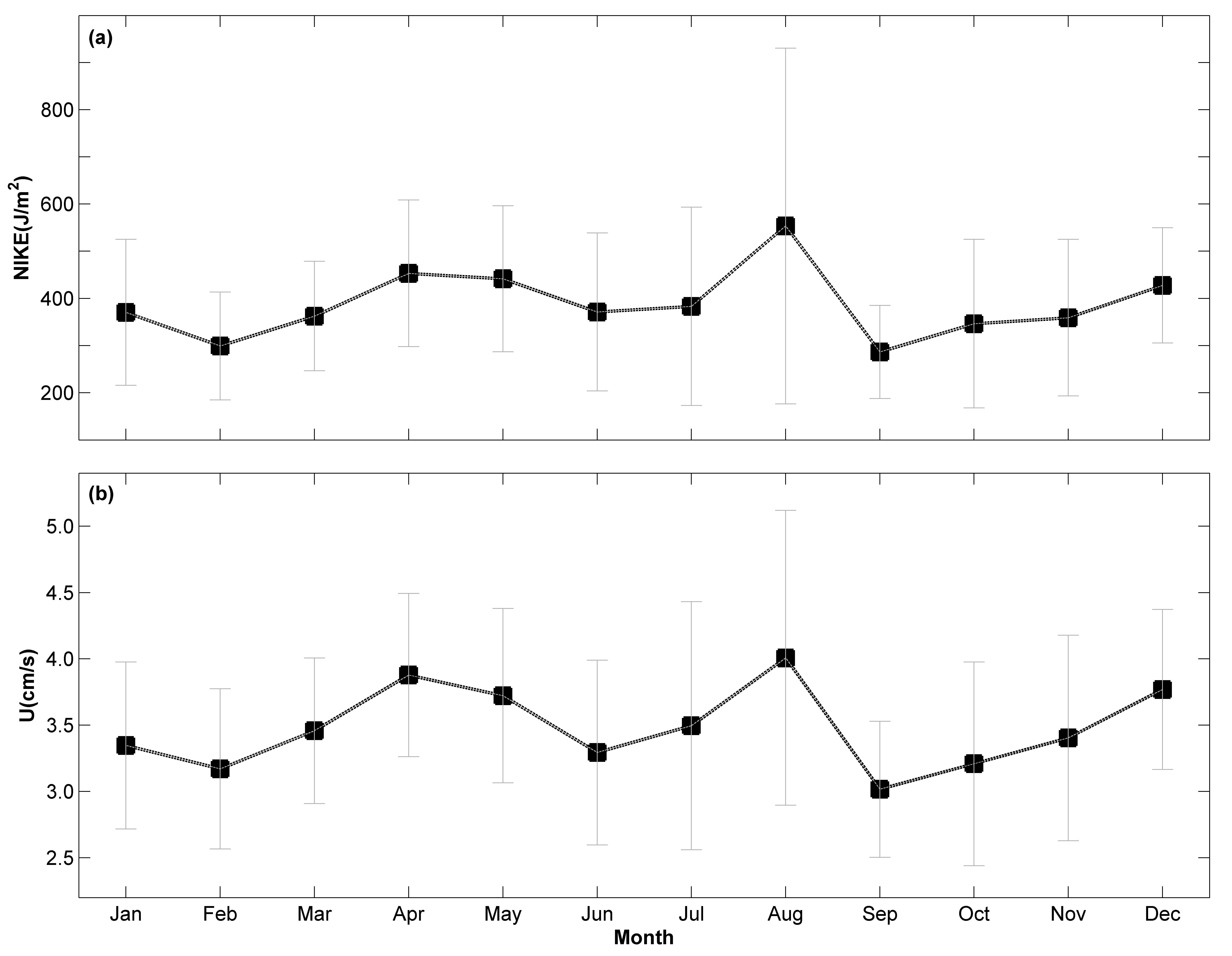
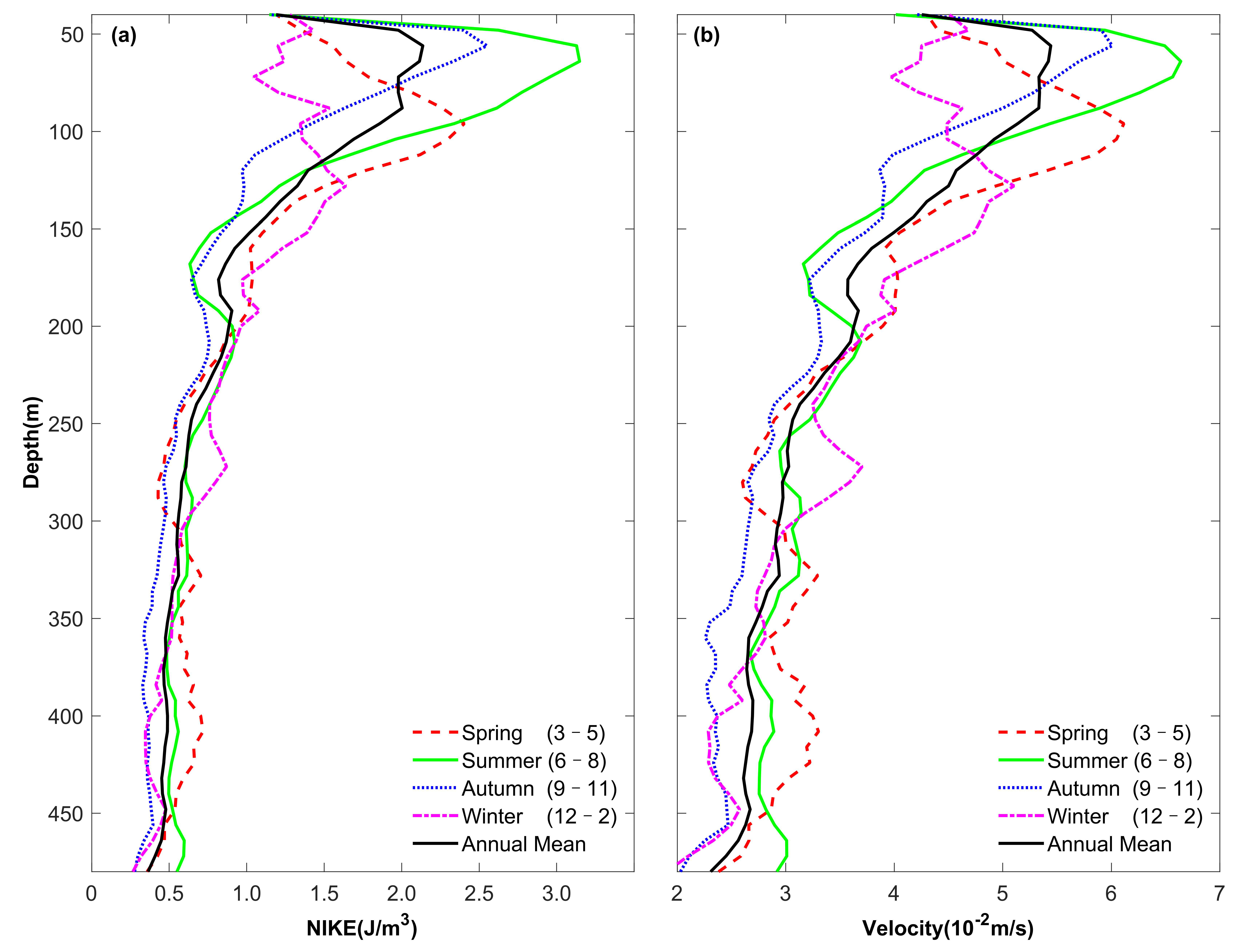
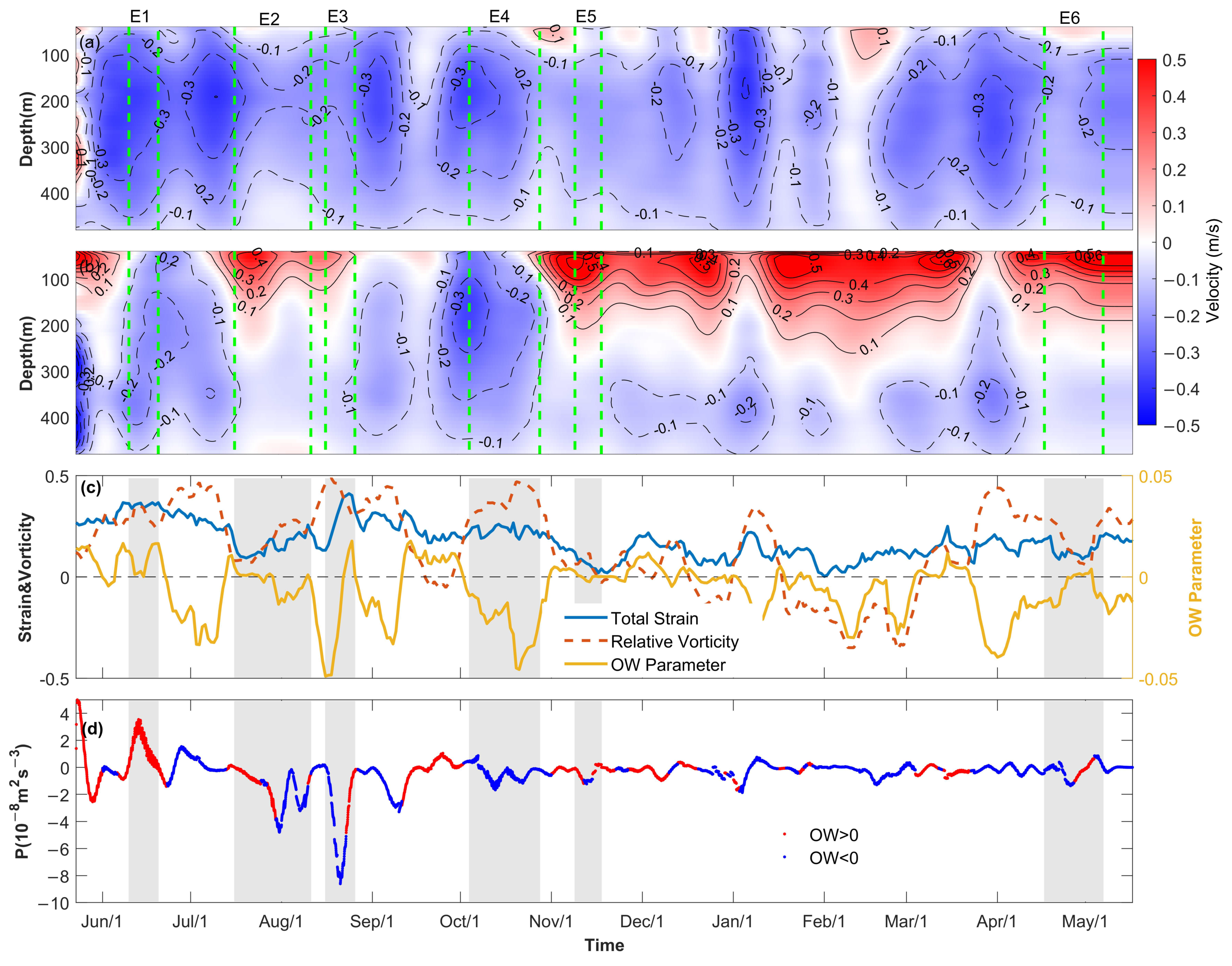
3.1. Seasonal Variation

The depth–time evolutions of NIKE are shown in Figure 2. The NIKE shows significant temporal intermittence, and notable high NIKE episodes mostly occur in the upper ocean, that is, above 150 m (Figure 2). The NIKE of most episodes exceeds 5.0 J/m³. There are several major large NIKE episodes, i.e., in mid-June of 2017, at the end of July 2017, in mid-October of 2017, and at the end of April, 2018. The time and depth ranges of six episodes of NIWs with depth-integrated NIKE exceeding one standard deviation are marked by the white rectangles. There are also NIWs episodes happening in the ocean interior, such as in December of 2017 and in January of 2018 (the dashed black rectangles in Figure 2). Large-amplitude NIKE events occurred in the upper 100 m during June to November, and they occurred below 100 m during December to May with tendencies that the magnitude and duration of each event decreased but the occurrence frequency increased.

There exists no significant seasonal variation of the depth-integrated (40–480 m) NIKE (Figure 3a). Higher NIKE appears in May and August, which is induced by energetic NIKE episodes. Wind-induced NIWs are caused primarily by the passage of storms. In the ECS, tropical cyclones mainly occur from May to September. Although the East Asia monsoon is strongest during winter, the NIKE is weaker due to the lack of rapid-changing tropical storm intensity winds. The annual mean depth-integrated NIKE is about 400 J/m². The depth mean amplitude of near-inertial velocities shows similar seasonal variation to the NIKE (Figure 3b). The annual mean near-inertial current amplitude from 40 to 480 m is about 3.50 cm/s. The most energetic NIKE and near-inertial velocity emerge in August with NIKE of 550 J/m² and near-inertial velocity amplitude of 4.00 cm/s.

Vertical propagation of NIKE is examined using rotary vertical wavenumber spectra (Figure 4). The NIWs are dominated by clockwise rotating with a depth component which suggests downward energy propagation. However, downward propagation of NIKE appears in different wavenumber bands for different seasons. In spring, downward propagation of NIKE occurs in 4 × 10⁻³ to 1 × 10⁻² cycles per stretched meter (cpsm) wavenumber band, and it is noteworthy that upward propagation of NIKE emerges in the (1−2) × 10⁻² cpsm wavenumber band. In summer, downward propagating NIKE occurs in a much wider wavenumber band, that is, less than 2 × 10⁻² cpsm. In autumn and winter, downward propagation of energy is concentrated in frequency bands of less than 1 × 10⁻² cpsm.

The seasonal mean NIKE and near-inertial currents show an evident subsurface intensified trend whose maximums range from 50 m to 100 m below the sea surface (Figure 5). Autumn has a maximum at a depth of 50 m, and in summer, the maximum deepens to 65 m. In spring, the NIKE maximum further deepens to about 100 m, and the NIKE maximum emerges at 130 m in winter. The NIKE and near-inertial currents below 200 m are almost unchanged, and resemble the trend of their annual mean. Summer has the most energetic NIWs, with NIKE of more than 3.00 J/m³, and near-inertial currents of 6.60 cm/s; spring and autumn have comparable maximum NIKE (2.50 J/m³) and near-inertial currents (6.00 cm/s). The near-inertial currents are relatively weaker in winter with maximum NIKE of 1.50 J/m³ and near-inertial currents of 5.00 cm/s.

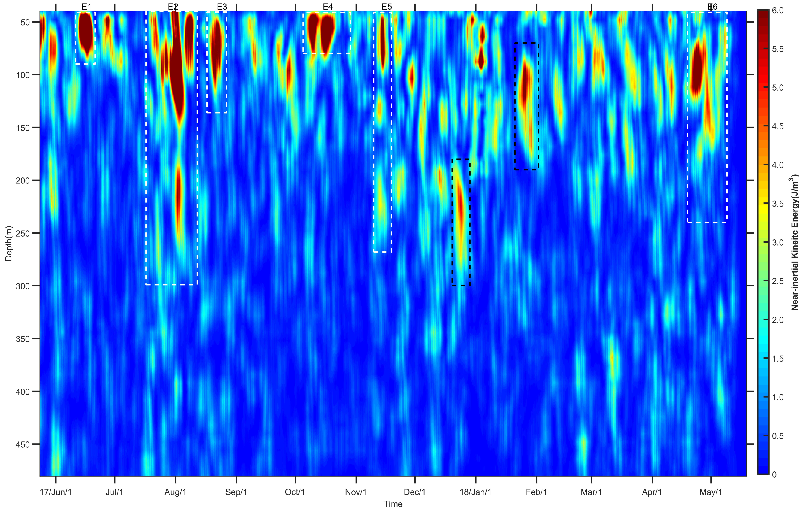
3.2. Episodes of NIWs

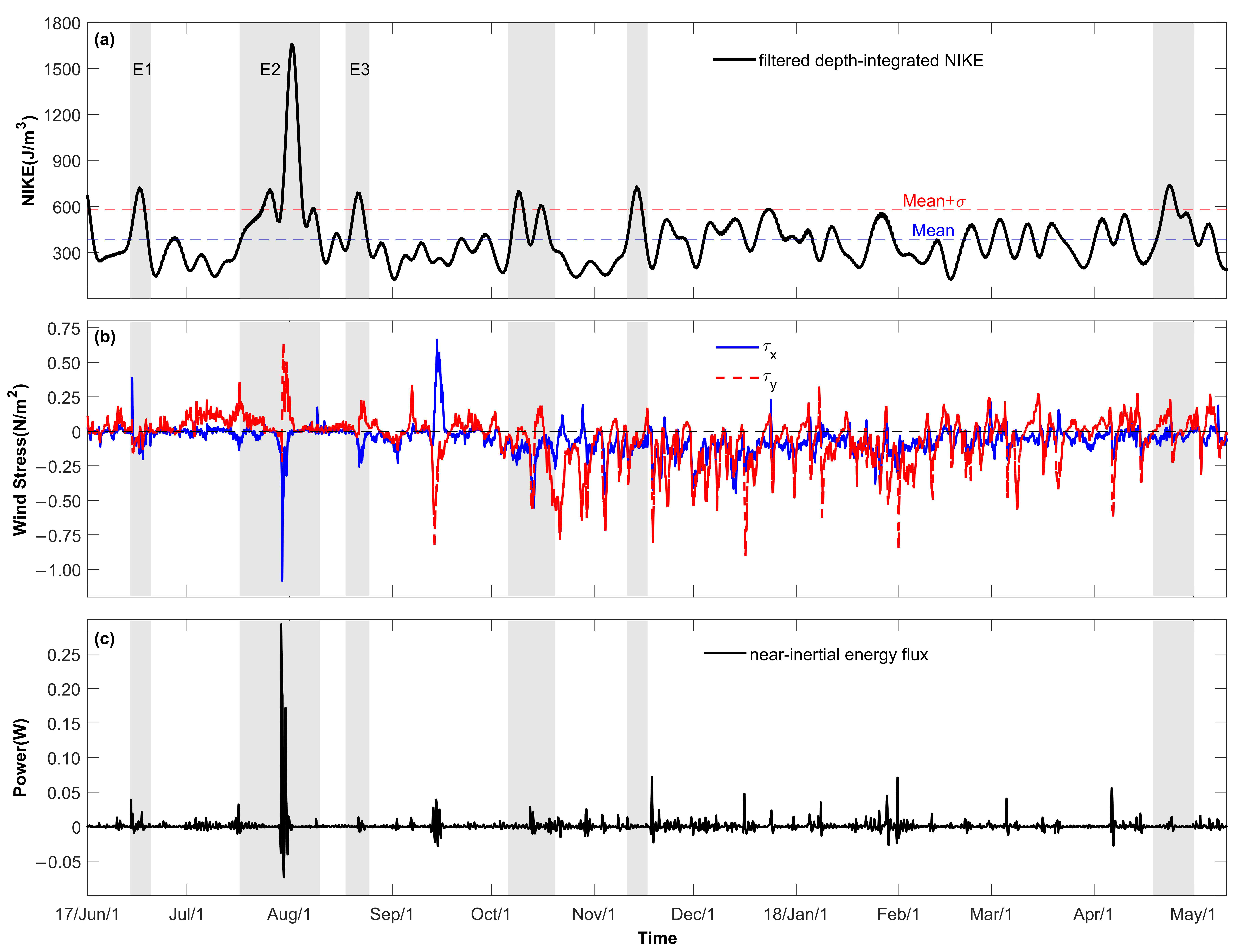
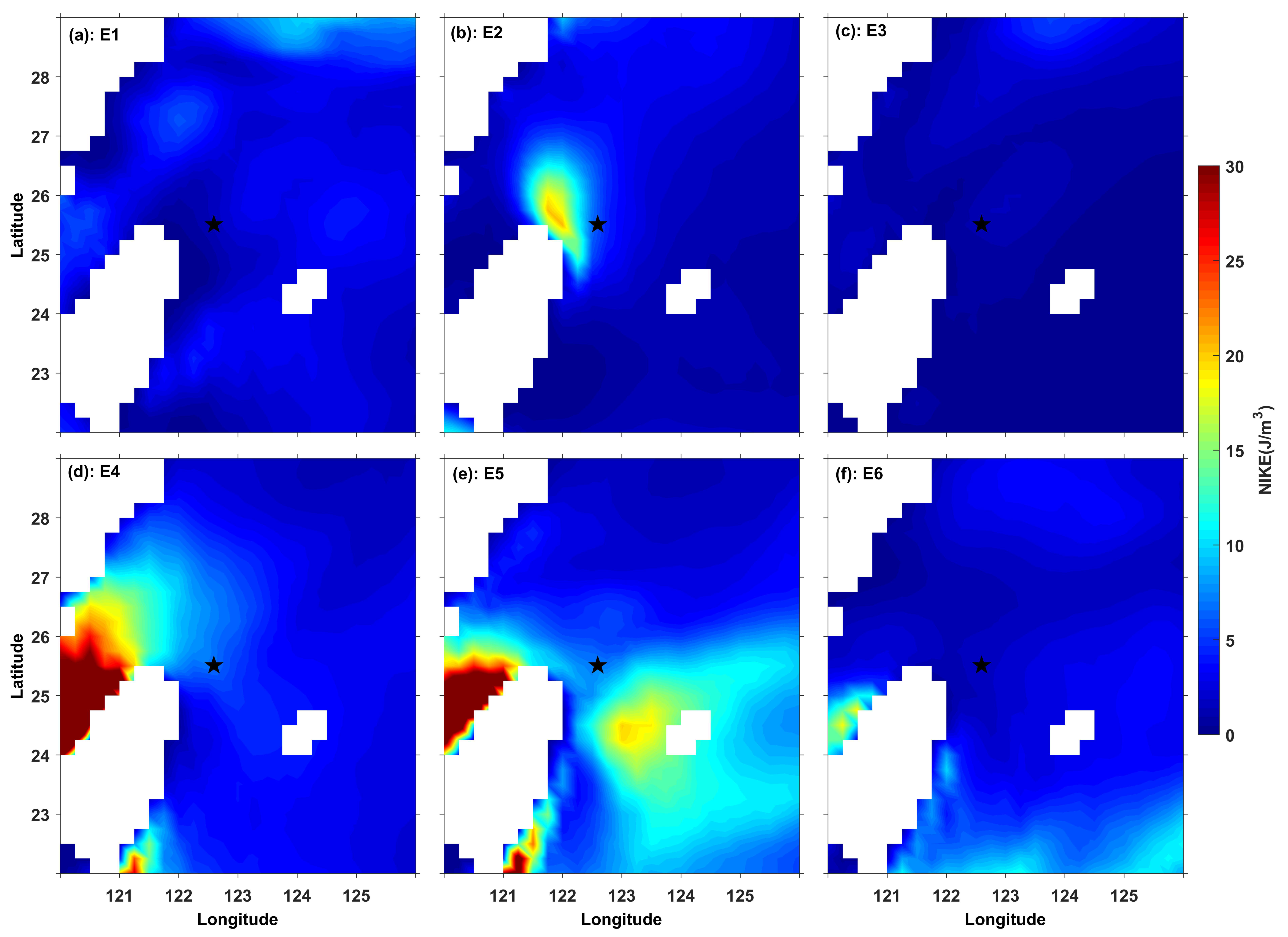
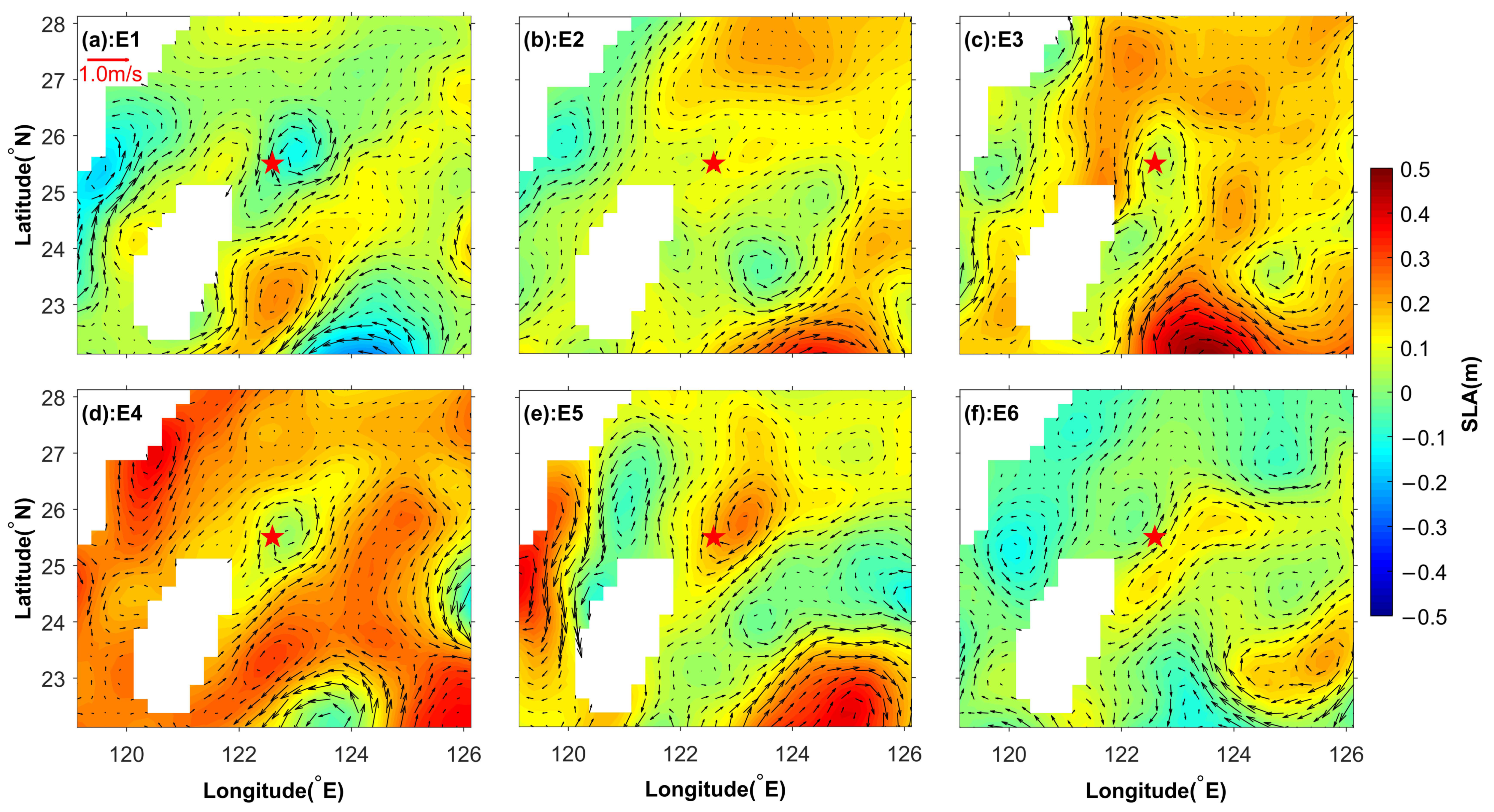
3.2.1. NIKE and Excitation Mechanism

The evolution of low-pass filtered NIKE, wind stress, and near-inertial energy flux from wind to the ocean is denoted in Figure 6. There are six episodes of NIWs with depth-integrated NIKE exceeding one standard deviation, which are coded E1 to E6 in chronological order (Figure 6). The occurrence of a large NIKE episode relates to the near-inertial variation of wind stress. The strongest episode, i.e., E2, occurring at the end of July and lasting to mid-August in 2017, was induced by typhoon Nesat. Besides the typhoon, a rapid enhancement of wind (in mid-June and mid-October) led to large NIKE episodes E1 and E4. However, there was no evident wind burst and near-inertial energy flux during episodes 3, 5, and 6. Episode 4 had two energy peaks, and the former one was not induced by wind; however, the latter one is related to wind.

Oceanic near-inertial responses to typhoons relate to oceanic initial states such as mixed layer depth, stratification, background currents, and characteristics of typhoons such as translation speed and the rotation of wind [12,33,34]. The wind field of typhoon Talim did not generate significant NIWs, which is distinctive from typhoon Nesat. The slow translation speed of Talim led to a smaller Mach number of 1.57, and the right-side track of Talim relative to the mooring station led to counterclockwise-rotating-dominated wind. Moreover, the mixed layer depth prior to the passage of Talim was 30 m, which was 10 m deeper than that of Nesat. The insignificant NIWs during Talim suggest that the right-side-passing and slow translating typhoon could not efficiently generate NIWs when coinciding with the deep mixed layer in the ECS.

Episodes 3 to 6 are not excited by the wind stress, and the probable reasons may be lateral propagation, parametric subharmonic instability, and loss of stability of large-scale circulation (herein the Kuroshio). Time-averaged mixed layer NIKE one day before each episode obtained from the slab model are presented in Figure 7. For episode 4, there is conspicuous NIKE west of the station with NIKE of about 15 J/m³ corresponding to near-inertial currents of 0.17 m/s. For episode 5, intensive NIKE emerges southeast of the mooring station, and the NIKE reaches 20 J/m³, corresponding to near-inertial currents of 0.20 m/s. The mode-1 internal waves near the station have a horizontal phase speed of about 1.30 m/s, which suggests that they can propagate more than 110 km within one day. Consequently, the occurrences of episodes 4 and 5 are resulted from lateral propagation of NIWs. However, before the occurrences of episode 3 and 6, there was no significant wind-induced mixed layer NIKE.

The parametric subharmonic instability (PSI) mechanism can also induce NIWs [35,36], and the latitude of the mooring station leads to a local inertial frequency close to the diurnal frequency. The bicoherence between the near-inertial (f) and D1 + f, D2 + f, D2-f zonal currents are shown in Figure 8. The bicoherence surpasses the 80% confidence level only for episode 1 around 130 m. However, episode 1 concentrated above 100 m (see Figure 9a), suggesting that PSI is not the stimulation mechanism of episode 1. The results suggest that the observed NIW episodes 3 and 6 are not induced by the PSI mechanism. The motivator of episodes 3 and 6 remains unknown. The Kuroshio intrudes on the mooring station during episode 6 according to AVISO sea level anomaly data. The loss balance of the Kuroshio and the related Kuroshio front are probable excitation mechanisms for episode 6 [37,38]. However, it is insufficient to testify concerning the mechanism of episode 6 with one site observation.

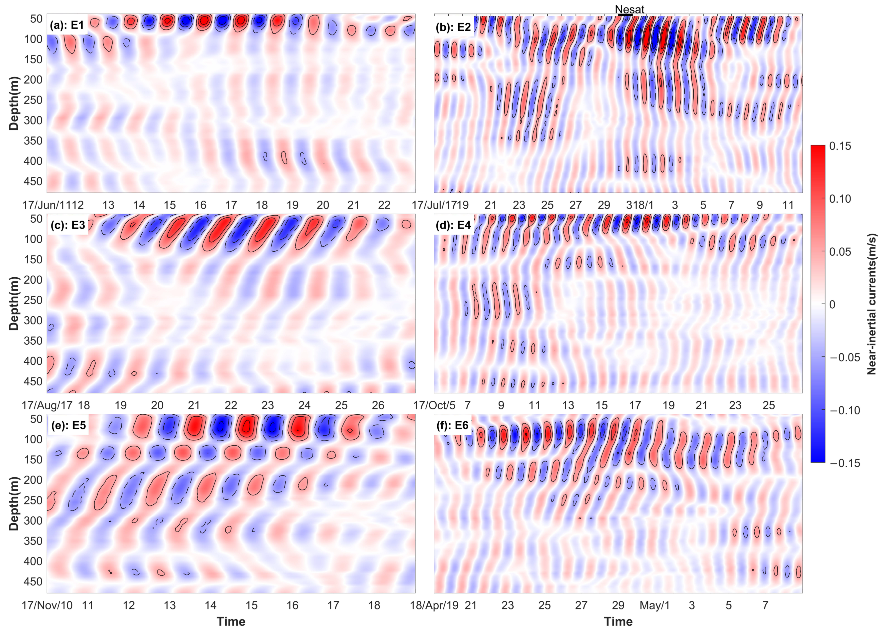
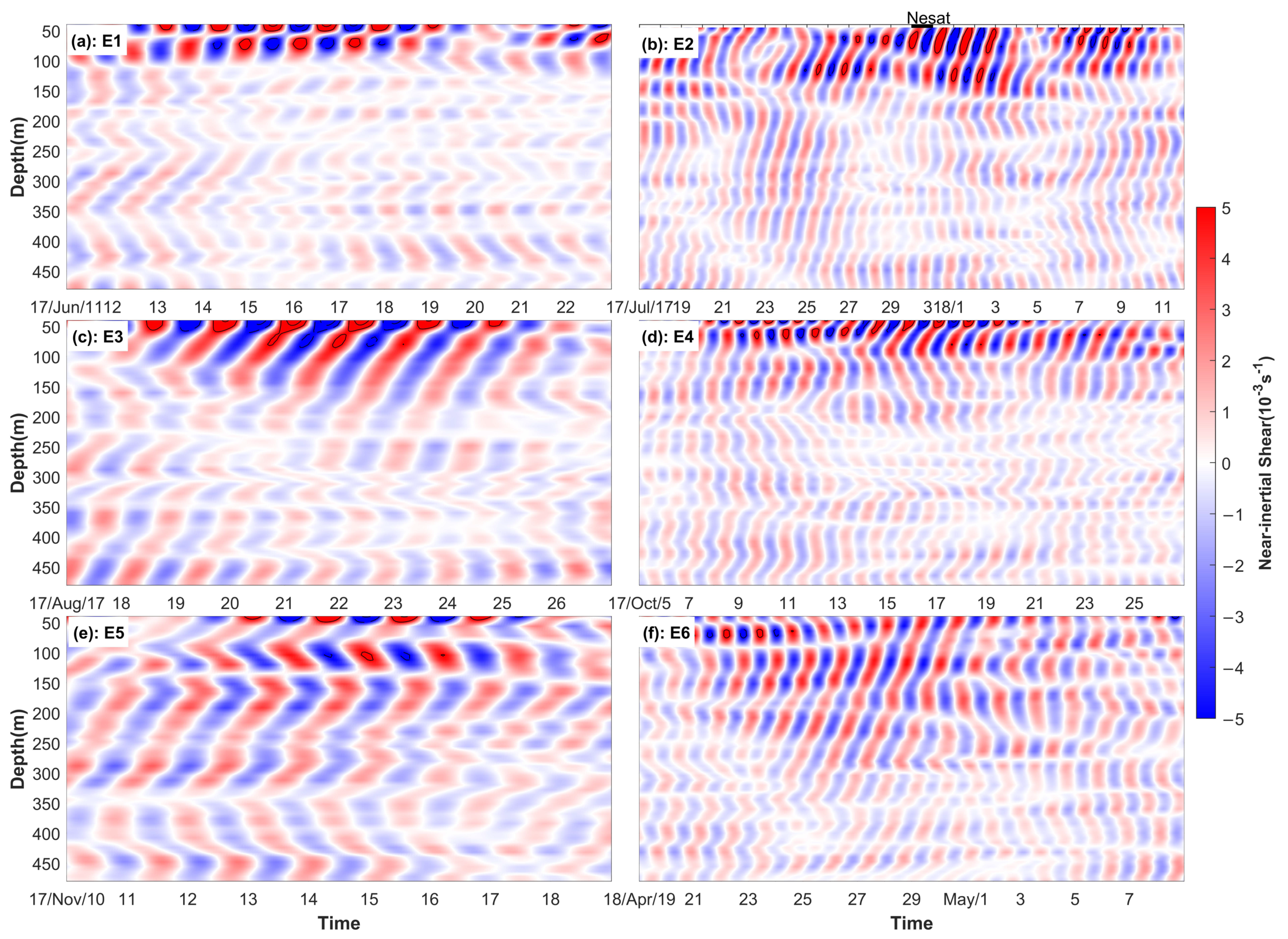
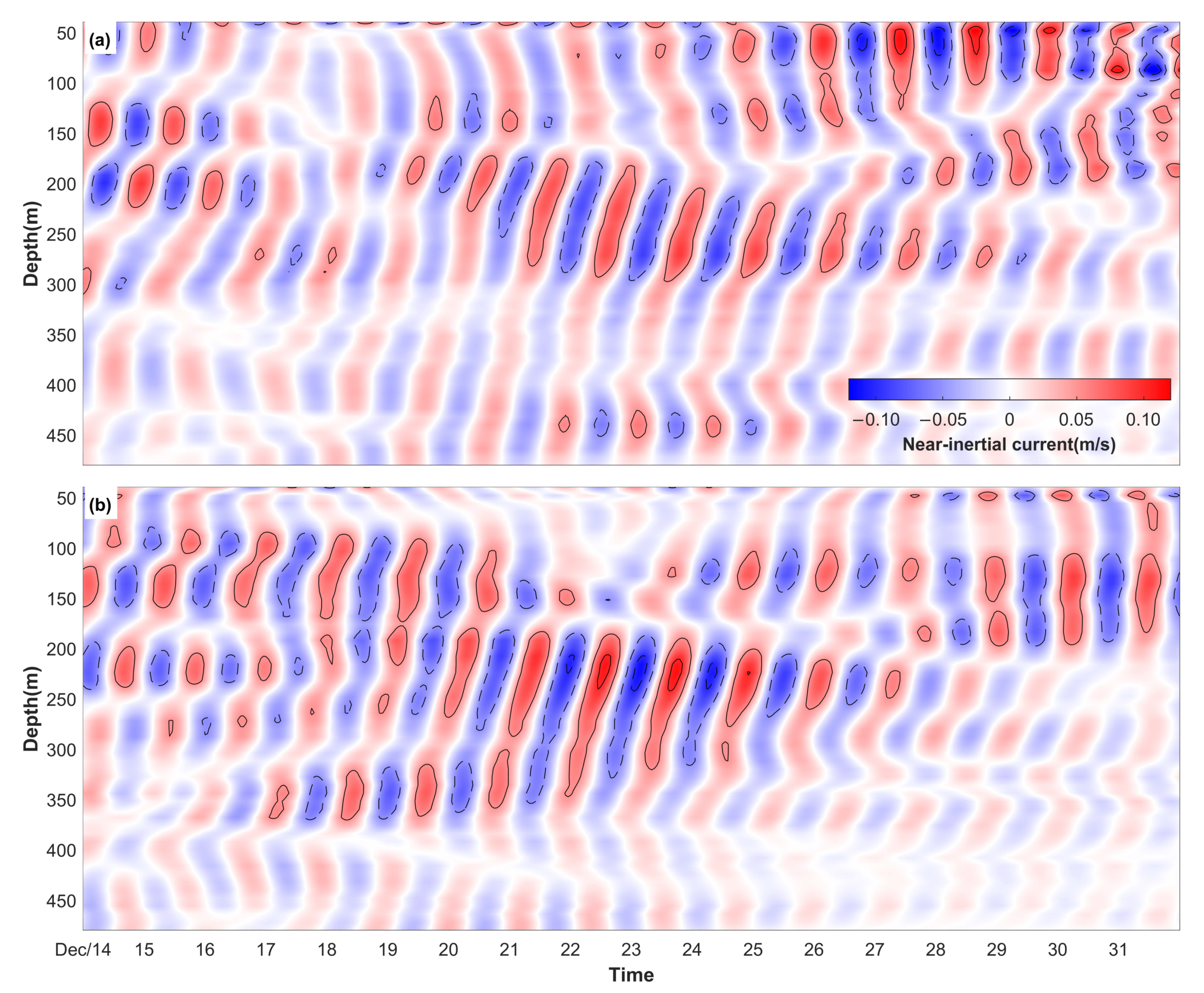
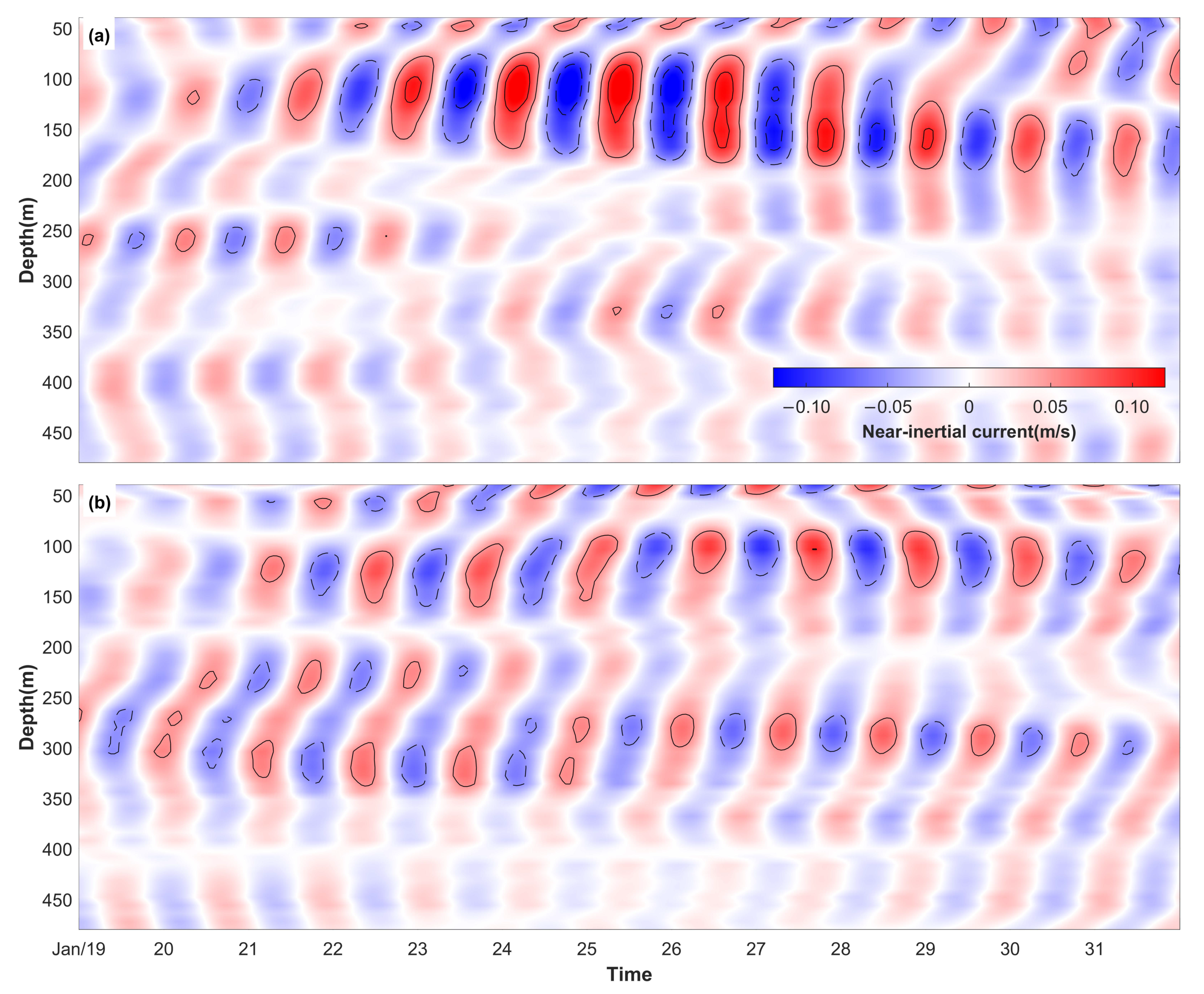
3.2.2. Near-Inertial Currents and Shear

The evolutions of near-inertial currents corresponding to each episode are shown in Figure 9. The near-inertial currents of episodes 1 to 6 show different temporal and spatial (vertical) patterns. Episodes 1 and 4 show subsurface intensified patterns with near-inertial currents reaching 0.15 m/s. Episodes 2, 3, 5, and 6 show baroclinic patterns with significant upward propagating vertical phase speed, i.e., downward propagating vertical group speed. The subsurface intensified near-inertial currents suggest an excitation source in the surface layer, which is consistent with the excitation mechanism of episodes 1 and 4. Moreover, episodes 5 and 6 show significant high mode patterns, that is, the near-inertial currents have frequent phase inversions in the vertical direction. Episodes 2, 5, and 6 cover rather extensive vertical ranges, and have near-inertial currents of 0.05 m/s at a depth of 300 m.

The vertical shear of near-inertial currents shows distinct patterns in comparison with the near-inertial currents (Figure 10). Strong vertical shear does not appear at the depth with the strongest near-inertial currents but appears where near-inertial currents are relatively small. The vertical shear of near-inertial currents reaches 0.005–0.010 s⁻¹. The high mode patterns of episodes 5 and 6 lead to prominent vertical shear. The patterns of near-inertial vertical shear verify the upward propagating vertical phase speed of NIWs, especially for episodes 2 to 6.

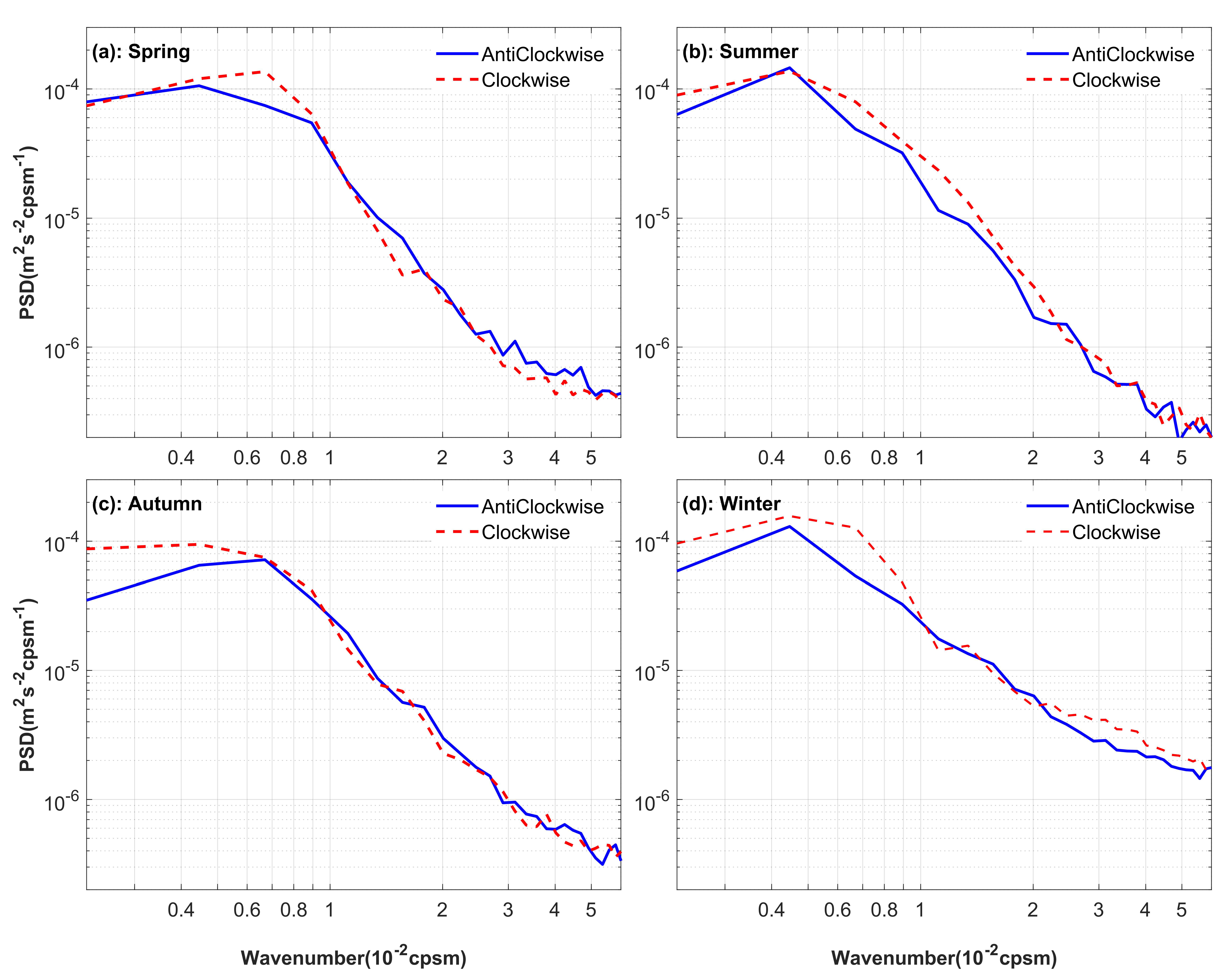
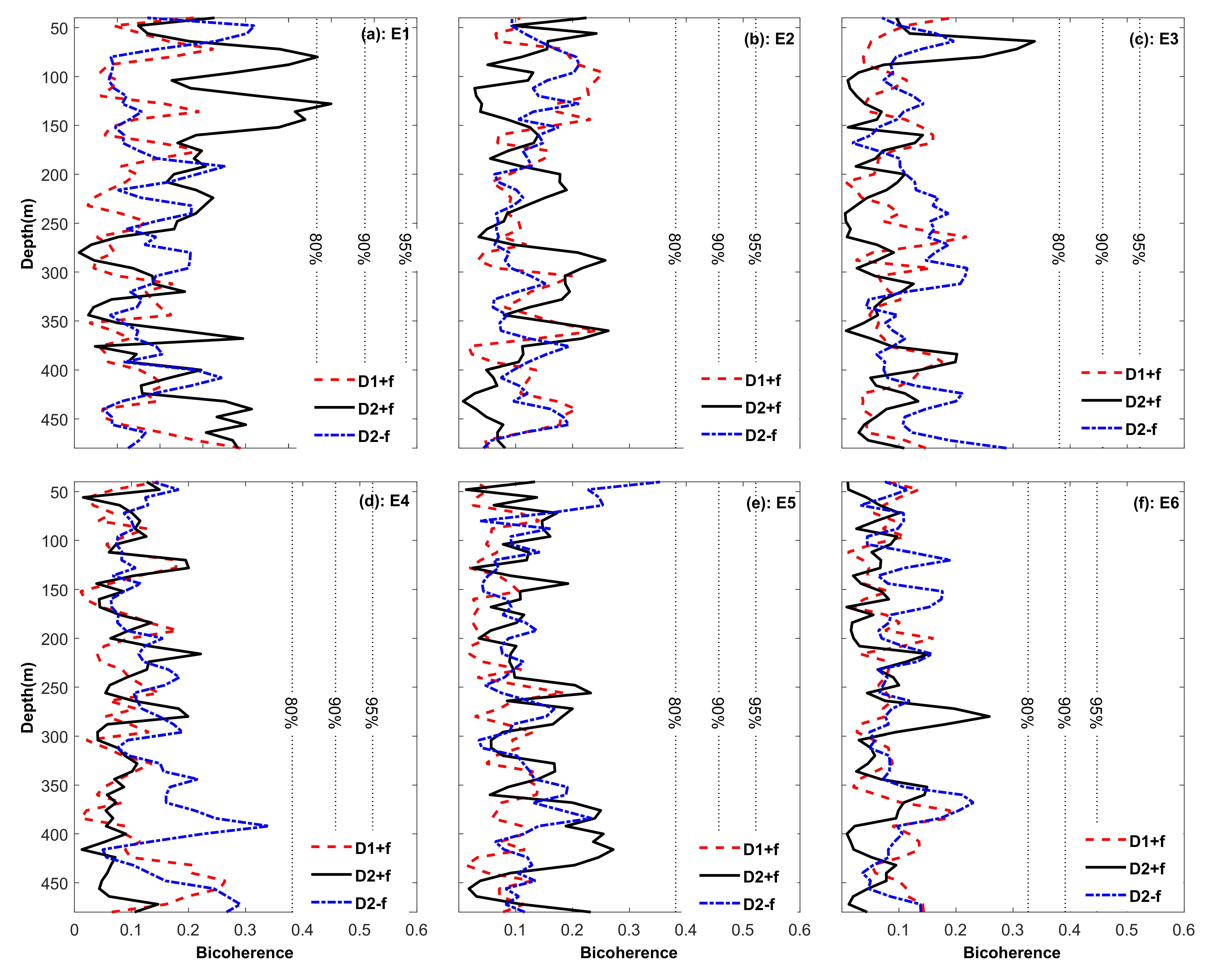
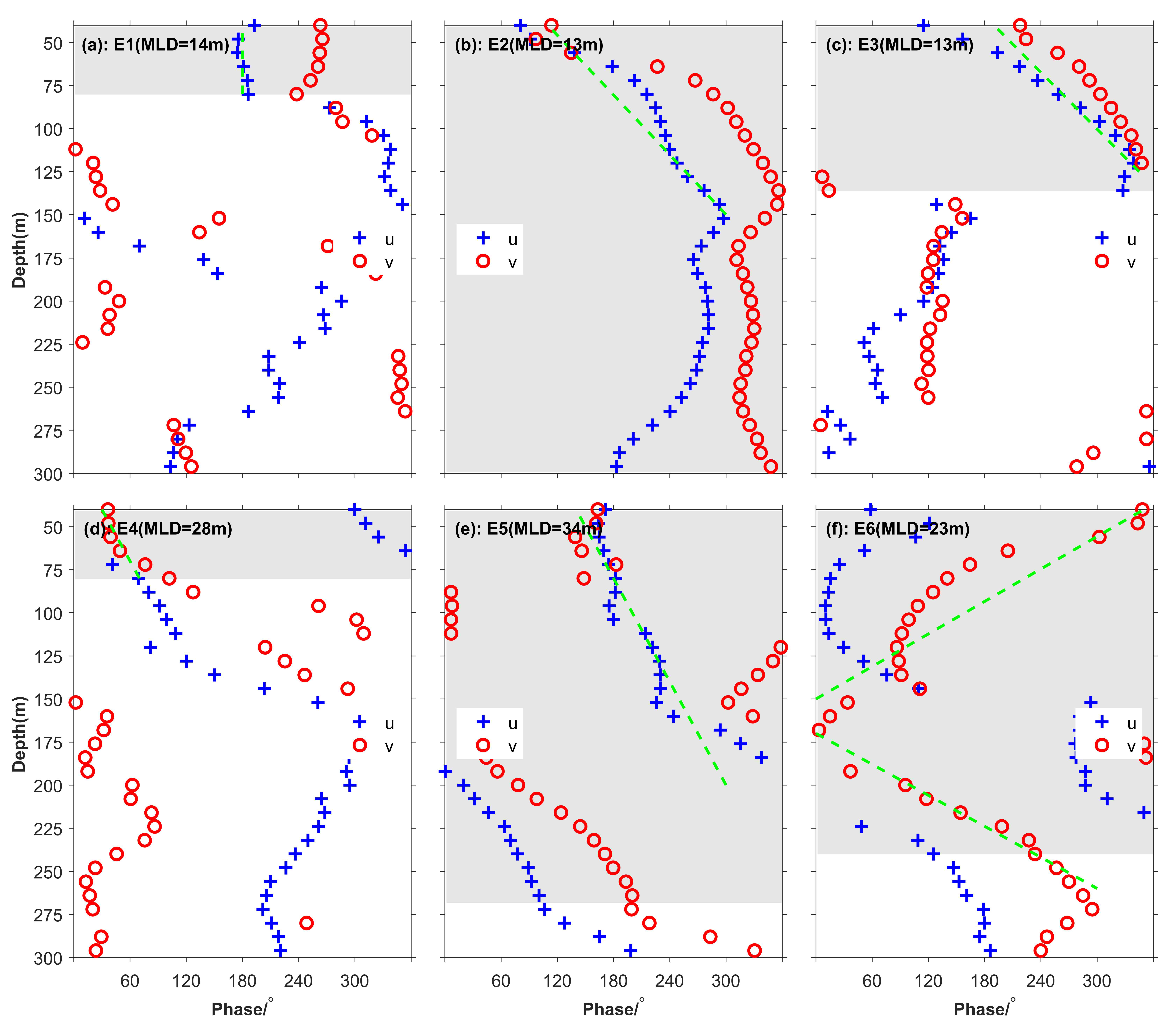
3.2.3. Frequency and Phase of NIWs

Vertical profiles of the NIWs’ frequency obtained through the plane wave fitting method are presented in Figure 11. The near-inertial currents are concentrated at certain depths, i.e., mostly the subsurface layer. In the following analysis, we focus on the depths with near-inertial currents stronger than 0.05 m/s. Episode 1 has a red-shifted frequency of 0.950f–0.975f, and has negligible vertical variation. Episode 2 also has a red-shifted frequency of 0.950f–0.975f, and the frequency varies slightly with depth. The frequency of episode 3 is also red-shifted, and has a vertical mean value of 0.970f. However, episode 4 has a blue-shifted frequency in the subsurface, and the frequency is about 1.035f. Episode 5 has a red-shifted frequency in most depths, which can reach 0.900f in the subsurface layer, and the vertical mean frequency is 0.950f. The frequency of episode 6 is red-shifted in the subsurface layer and below 150 m; however, it has a slight blue-shift between 75 m to 150 m.

Figure 12 shows vertical profiles of the phase of the observed near-inertial waves. The phase of episode 1 is approximately uniform in the subsurface layer, that is, from 40 m to 80 m, and there is a 90° phase difference between the zonal and the meridional near-inertial currents. The temporal-mean mixed layer depth during episode 1 is 14 m, suggesting that the phase of episode 1 in the thermocline hardly changes vertically, which is distinctive from most downward propagating NIWs. For episodes 2 to 4, the phases show a depth-leading trend, which corresponds to upward vertical phase speed and downward vertical group speed. The phase of episode 5 presents a uniform structure in the subsurface layer and a depth-leading trend in the ocean interior. The phase of episode 6 shows a subsurface-leading trend in the subsurface layer and a depth-leading trend in the ocean interior, suggesting that there are both upward and downward propagations of vertical group speed (energy). Based on the vertical profiles, the vertical phase speeds of episodes 2 to 5 are estimated to be 11.84 m/h, 6.10 m/h, 4.85 m/h, 8.62 m/h, respectively. The upward phase and downward vertical phase speeds of episode 6 are 4.49 m/h and 5.92 m/h, respectively.

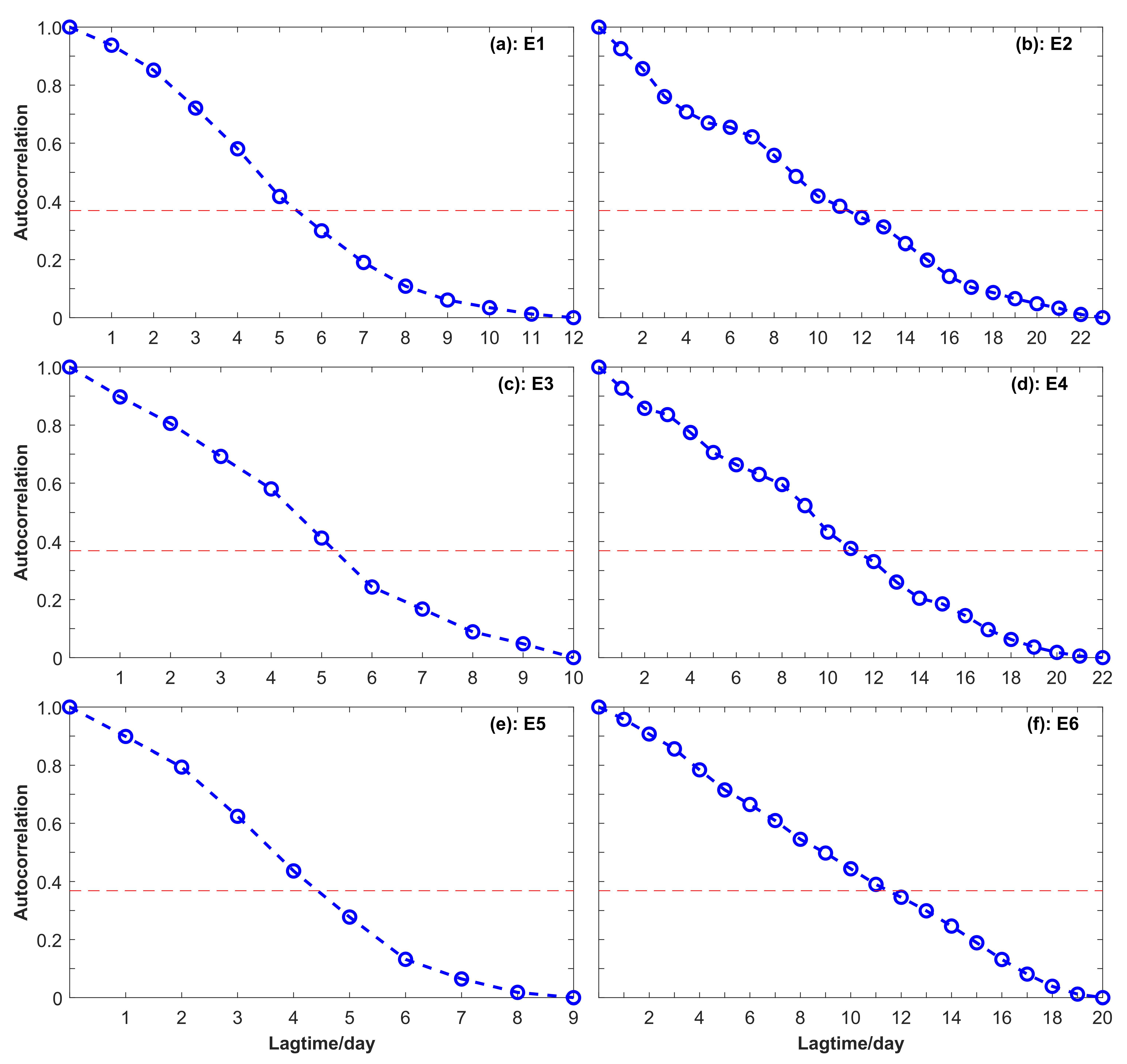
3.2.4. E-Folding Time of NIWs

Autocorrelations of the depth-integrated NIKE are shown in Figure 13. The e-folding time of each NIWs episodes are estimated through the autocorrelations, and the e-folding times of episodes 1 to 6 are 5 days, 11 days, 5 days, 11 days, 4 days, and 11 days, respectively. Episodes 2 and 4 have e-folding times of more than 10 days because they are induced by two consecutive wind bursts (Figure 6c). The persistent time of NIWs is related to background vorticity, especially the vorticity of mesoscale eddies. Mesoscale eddies around the mooring station are detected according to AVISO sea level anomaly data (Figure 14). The occurrences of episodes 1 and 3–6 are accompanied by mesoscale eddies. Episodes 1, 3, and 4 coincide with anticlockwise eddies (positive relative vorticity) which facilitate dispersion of NIWs. Consequently, episodes 1 and 3 have short e-folding times; however, episode 4 has an e-folding time of 11 days because it has two peaks that are induced by lateral propagation and wind burst. Episodes 5 and 6 coincide with clockwise eddies (negative relative vorticity), which lead to trapping of NIWs. Consequently, episode 6 has a long e-folding time of 11 days; however, episode 5 has an e-folding time of only 4 days which results from the high mode characteristics of episode 5 (see Figure 9e). The frequencies, vertical phase speed, and e-folding time of each episode are summarized in

Table 1. Depth-mean frequencies, vertical phase speed, and e-folding time of each episode.

Episode	Frequency (f)	Phase Speed (m/h)	E-Folding Time (Days)
1	0.960	NA 1	5
2	0.960	11.84	11
3	0.970	6.10	5
4	1.035	4.85	11
5	0.950	8.62	4
6	0.960	4.49 2/5.92 3	11

¹ NA denotes not applicable; ² upward propagating phase speed; ³ downward propagating phase speed.

.

4. Discussion

In the southeastern ECS, NIWs have annual mean and maximum horizontal velocities of 3.50 cm/s and 15 cm/s, respectively. They occur frequently and show significant temporal intermittence because NIWs are dominated by episodes. During the observation period, the NIKE shows no significant seasonal variation. Rapid-changing atmospheric wind and lateral propagation, respectively, drive two NIWs episodes, and excitation mechanisms of the remaining two episodes are unknown. According to satellite altimeter remote sensing geostrophic current data, the Kuroshio intruded on the ECS and influenced the background current of the station during the observation period. It is noteworthy that the right-side-passing and slow-moving typhoon Talim did not induce significant NIWs; however, the left-side-passing and rapid-moving typhoon Nesat induced energetic NIWs. The counterclockwise-rotating-dominated wind as Talim passed over from the right side of the mooring station, the slow-translating speed of typhoon Talim and the deeper mixed layer caused the ineffective excitation of near-inertial waves [33,34].

The observed NIWs episodes can be low mode NIWs and high mode NIWs. The vertical shear of near-inertial currents can reach 0.01 s⁻¹, especially for high mode NIWs. The frequency of NIWs can be modified by background vorticity and background current [39,40,41]. Background vorticity can modify the effective Coriolis frequency ($f_{eff}$) as:

$$f_{eff}=f+\frac{\zeta }{2},$$

(13)

where f is local inertial frequency, and $\zeta$ is the background vorticity. Kuroshio can enable poleward-propagating NIWs along the right-hand side of the Kuroshio path where Kuroshio has negative relative vorticity [42]. Our observations were located on the left-hand side of Kuroshio, and the relative vorticity was positive during all episodes (Figure 15c). However, all episodes except episode 4 have red-shifted frequencies, which is contrary to the positive background relative vorticity.

The Doppler shift induced by the background currents (herein the Kuroshio) is a probable mechanism for the red-shift. The Doppler shift can be estimated according to

$${\omega }_0=\mathsf{\omega }-\left(\overrightarrow{k}·\overrightarrow{V}\right)$$

(14)

where ${\omega }_0$ is the intrinsic frequency, and $\left(\overrightarrow{k}·\overrightarrow{V}\right)$ is the Doppler shift by background currents. The Kuroshio has a velocity of about 0.20–0.50 m/s during episodes 1–6 (Figure 15a,b), and considering typical near-inertial waves with wavenumber of 6.28 × 10⁻⁵ m⁻¹ (corresponding to a wave length of O (100 km)). Assuming the horizontal phase speed of NIWs parallels the Kuroshio flow, the corresponding Doppler shift is $\overrightarrow{k}·\overrightarrow{V}=-\left(0.20~0.50\right)f$, and the negative Doppler shift results from northward-dominated Kuroshio (dominated along the Kuroshio path flow, see Figure 15a,b) and southward propagating NIWs (lower inertial frequency at lower latitude allows southward free propagation of NIWs). The relative vorticity during episodes 1–6 varied from 0.10f to 0.50f, corresponding to an effective Coriolis frequency of (1.05–1.25)f. Consequently, the Doppler shift is capable of resulting in a red-shift to the observed NIWs.

Low-frequency flows can transfer energy to near-inertial waves when and where the strain of low-frequency flows dominates its relative vorticity [43,44,45]. Based on the AVISO dataset, strain and relative vorticity ($\zeta$) of geostrophic flows at the station are calculated according to:

$$\begin{array}{l}{S}_n=\frac{\partial U}{\partial x}-\frac{\partial V}{\partial y}\\ S_s=\frac{\partial V}{\partial x}+\frac{\partial U}{\partial y}\\ \zeta =\frac{\partial V}{\partial x}-\frac{\partial U}{\partial y}\end{array}$$

(15)

where S_n and S_s are normal and shear strain, U and V are zonal and meridional geostrophic currents from the AVISO dataset. The relative importance of total strain and relative vorticity is diagnosed with the Okubo–Weiss parameter, defined as:

$${\alpha }^2=\frac{1}{4}\left(S_n^2+S_s^2-{\zeta }^2\right)$$

(16)

The rate of energy transfer from the mesoscale field to NIWs is estimated following [44]:

$$P=-0.5\left(〈uu〉-〈vv〉\right)S_n-〈uv〉S_s$$

(17)

where the angle brackets represent the running mean over three inertial periods. During episode 1, the total strain exceeded relative vorticity, resulting in a positive Okubo–Weiss parameter and a positive rate of energy transfer of about 1.0 × 10⁻⁸ m²s⁻³ (Figure 15c,d). For episodes 2–6, there are no significant energy transfers from mesoscale field to NIWs.

There were interesting NIWs episodes that happened in the ocean interior, i.e., in December and January (see the black rectangles in Figure 2). We analyzed characteristics of the two NIKE events, and the near-inertial currents of the two events are shown in Figure 16 and Figure 17. The NIWs in December were concentrated from 150 m to 300 m and show an evident depth-leading vertical phase, which indicates downward propagation of energy. The depth mean frequency and vertical phase speed of NIWs in December are 0.975f and 10.08 m/h. However, the NIWs in January were concentrated from 80 m to 200 m, and the NIWs in January have a vertical mean frequency of 0.925f and a vertical phase speed of 19.12 m/h. The occurrences of NIWs events in December and January were accompanied by strong Kuroshio currents (see Figure 15a,b), and consequently the generation and frequency shift of them may relate to the Kuroshio [46].

5. Conclusions

Based on in-situ observations as well as reanalysis and satellite data, the mechanism and characteristics of NIWs on the continental slope of the southeast ECS were examined. The in-situ observations lasted for almost 1 year, and there were six detected energetic episodes of NIWs. Episode 1 was the most energetic one, which is induced by wind burst, and episode 2 was generated by the wind of typhoon Nesat. Episode 4 was excited by a combination of lateral propagation and wind burst, and episode 5 was generated by lateral propagation. The generation mechanisms of episodes 3 and 6 remain unknown. It is noteworthy that the right-side-passing (with counterclockwise-rotating-dominated wind) and slow-moving typhoon Talim with a Mach number of 1.57 does not induce significant NIWs in the ECS.

The depth-integrated NIKE does not show significant seasonal variation. The annual mean depth-integrated NIKE is 400 J/m², and the annual mean depth-integrated near-inertial current amplitude is 3.50 cm/s. According to the rotary vertical wavenumber spectra, downward propagation of NIKE is evident in a smaller wavenumber band (less than 2 × 10⁻² cpsm). Vertically, the NIKE is subsurface-intensified from 50 m to 100 m. The depth of maximum seasonal mean NIKE is largest in winter (130 m), and smallest in autumn (50 m). Based on vertical profiles of seasonal mean NIKE, summer has the most energetic NIWs with NIKE values of more than 3.00 J/m² and near-inertial current of 6.60 cm/s, and winter has the weakest NIWs with NIKE of 1.50 J/m² and near-inertial current of 5 cm/s.

Episode 1 shows a vertically uniform phase profile, and episodes 2 to 6 show evident baroclinic vertical patterns. Moreover, episodes 5 and 6 show high mode vertical patterns. The vertical shear of near-inertial currents can reach 0.01 s⁻¹. The frequencies of the observed NIWs are mostly red-shifted; however, episode 4 is blue-shifted and 6 has both blue-shift and red-shift. The background vorticity is positive during most episodes. The frequency shifts are related to the Doppler shift induced by the Kuroshio. The upward vertical phase speeds of episodes 2 to 5 are 11.81 m/h, 6.10 m/h, 4.85 m/h, and 8.62 m/h, respectively. Episode 6 shows downward vertical phase speed in the upper layer and upward vertical phase speed in the deep layer, and the phase speeds are 5.92 m/day and 4.49 m/h, respectively. The e-folding time of the observed NIWs is 4 to 11 days. Episodes 2 and 4 have e-folding times of 11 days because they were induced by two consecutive wind bursts, and 6 is influenced by a clockwise mesoscale eddy with negative vorticity. Episode 5 has an e-folding time of 4 days which results from its high mode feature.

The Kuroshio, a strong western boundary current, influences many oceanic processes of the ECS. The excitation mechanism of ECS NIWs can be a typhoon, wind burst, lateral propagation, and an energy transfer from low-frequency flows to NIWs also has a contribution. There exists a positive rate of energy transfer from low-frequency flows to NIWs when and where the total strain of Kuroshio exceeds its relative vorticity. On the left-hand side of Kuroshio, the background relative vorticity is always positive, however, the observed NIWs usually have red-shifted frequencies. The Doppler shift induced by Kuroshio is estimated to be sufficient to induce the red-shift of NIWs. Recent research reveals that NIWs around the Kuroshio can be induced by inertial instability and have a significant influence on oceanic turbulent layers and nutrient supply [46,47,48]. The Kuroshio mainstream meanders in the southeastern ECS and the modification of Kuroshio on the generation and propagation of NIWs in the ECS need further research.

References

1. Watanabe, M.; Hibiya, T. Global estimates of the wind-induced energy flux to inertial motions in the surface mixed layer. Geophys. Res. Lett. 2002, 29, 1239. [Google Scholar] [CrossRef]
2. Furuichi, N.; Hibiya, T.; Niwa, Y. Model-predicted distribution of wind-induced internal wave energy in the world’s oceans. J. Geophys. Res. Oceans 2008, 113, C09034. [Google Scholar] [CrossRef]
3. Simmons, H.L.; Alford, M.H. Simulating the long-range swell of internal waves generated by ocean storms. Oceanography 2012, 25, 30–41. [Google Scholar] [CrossRef]
4. Rimac, A.; von Storch, J.S.; Eden, C.; Haak, H. The influence of high-resolution wind stress field on the power input to near-inertial motions in the ocean. Geophys. Res. Lett. 2013, 40, 4882–4886. [Google Scholar] [CrossRef]
5. Egbert, G.D.; Ray, R.D. Significant dissipation of tidal energy in the deep ocean inferred from satellite altimeter data. Nature 2000, 405, 775–778. [Google Scholar] [CrossRef] [PubMed]
6. Wunsch, C. The work done by the wind on the oceanic general circulation. J. Phys. Oceanogr. 1998, 28, 2332–2340. [Google Scholar] [CrossRef]
7. Alford, M.H.; MacKinnon, J.A.; Simmons, H.L.; Nash, J.D. Near-inertial internal gravity waves in the ocean. Annu. Rev. Mar. Sci. 2016, 8, 95–123. [Google Scholar] [CrossRef] [Green Version]
8. Chen, Z.; Chen, S.; Liu, Z.; Xu, J.; Xie, J.; He, Y.; Cai, S. Can tidal forcing alone generate a GM-like internal wave spectrum. Geophys. Res. Lett. 2019, 46, 14644–14652. [Google Scholar] [CrossRef]
9. Hu, Q.; Huang, X.; Zhang, Z.; Zhang, X.; Xu, X.; Sun, H.; Zhou, C.; Zhao, W.; Tian, J.W. Cascade of internal wave energy catalyzed by eddy-topography interaction in the deep South China Sea. Geophys. Res. Lett. 2019, 47, e2019GL086510. [Google Scholar] [CrossRef]
10. Soares, S.M.; Natarov, A.; Richards, K.J. Internal swells in the tropics: Near-inertial waves energy fluxes and dissipation during CINDY. J. Geophys. Res. Oceans 2016, 121, 3297–3324. [Google Scholar] [CrossRef] [Green Version]
11. Chen, G.X.; Xue, H.J.; Wang, D.X.; Xie, Q. Observed near-inertial kinetic energy in the northwestern South China Sea. J. Geophys. Res. Oceans 2013, 118, 4965–4977. [Google Scholar] [CrossRef] [Green Version]
12. Yang, B.; Hou, Y.J.; Hu, P.; Liu, Z.; Liu, Y.H. Shallow Ocean response to tropical cyclones observed on the continental shelf of the northwestern South China Sea. J. Geophys. Res. Oceans 2015, 120, 3817–3836. [Google Scholar] [CrossRef]
13. Subeesh, M.P.; Unnikrishnan, A.S. Observed internal tides and near-inertial waves on the continental shelf and slope off Jaigarh, central west coast of India. J. Mar. Syst. 2016, 157, 1–19. [Google Scholar] [CrossRef]
14. Cao, A.; Guo, Z.; Song, J.; Lv, X.; He, H.; Fan, W. Near-inertial waves and their underlying mechanisms based on the South China Sea internal wave experiment (2010–2011). J. Geophys. Res. Oceans 2018, 123, 5026–5040. [Google Scholar] [CrossRef]
15. Jeon, C.; Park, J.H.; Park, Y.G. Temporal and spatial variability of near-inertial waves in the East/Japan Sea from a high-resolution wind-forced ocean model. J. Geophys. Res. Oceans 2019, 124, 6015–6029. [Google Scholar] [CrossRef]
16. Kawaguchi, Y.; Wagawa, T.; Igeta, Y. Near-inertial internal waves and multiple-inertial oscillations trapped by negative vorticity anomaly in the central Sea of Japan. Prog. Oceanogr. 2020, 181, 102240. [Google Scholar] [CrossRef]
17. Park, J.J.; Kim, K.; Schmitt, R.W. Global distribution of the decay timescale of mixed layer inertial motions observed by satellite-tracked drifters. J. Geophys. Res. Oceans 2009, 114, C11010. [Google Scholar] [CrossRef] [Green Version]
18. Alford, M.H.; Whitmont, M. Seasonal and spatial variability of near-inertial kinetic energy from historical moored velocity records. J. Phys. Oceanogr. 2007, 37, 2022–2037. [Google Scholar] [CrossRef]
19. Silverthorne, K.E.; Toole, J.M. Seasonal kinetic energy variability of near-inertial motions. J. Phys. Oceanogr. 2009, 39, 1035–1049. [Google Scholar] [CrossRef]
20. Yang, J.; Zhou, S.H.; Zhou, J.X.; Lynch, J.F. Internal wave characteristics at the ASIAEX site in the East China Sea. IEEE J. Ocean. Eng. 2004, 29, 1054–1060. [Google Scholar] [CrossRef]
21. Li, X.F.; Zhao, Z.X.; Han, Z.; Xu, L.X. Internal solitary waves in the East China Sea. Acta Oceanol. Sin. 2008, 27, 51–59. [Google Scholar]
22. Cho, C.; Nam, S.H.; Song, H. Seasonal variation of speed and width from kinematic parameters of mode-1 nonlinear internal waves in the northeastern East China Sea. J. Geophys. Res. Oceans 2016, 121, 5942–5958. [Google Scholar] [CrossRef]
23. Nam, S.; Kim, D.J.; Lee, S.W.; Kim, B.G.; Kang, K.M.; Cho, Y.K. Nonlinear internal wave spirals in the northern East China Sea. Sci. Rep. 2018, 8, 3473. [Google Scholar] [CrossRef]
24. Park, J.H.; Lie, H.J.; Guo, B.H. Observation of semi-diurnal internal tides and near-inertial waves at the shelf break of the East China Sea. Ocean. Polar Res. 2011, 33, 409–419. [Google Scholar] [CrossRef] [Green Version]
25. Noh, S.S.; Seung, Y.H.; Lim, E.; You, H. Characteristics of semi-diurnal and diurnal currents at a KOGA station over the East China Sea shelf. Ocean. Polar Res. 2014, 36, 49–57. [Google Scholar] [CrossRef] [Green Version]
26. Lozovatsky, I.; Jinadasa, P.; Lee, J.H.; Fernando, H.J. Internal waves in a summer pycnocline of the East China Sea. Ocean. Dyn. 2015, 65, 1051–1061. [Google Scholar] [CrossRef]
27. Yang, W.; Wei, H.; Zhao, L. Parametric subharmonic instability of the semidiurnal internal tides at the East China Sea shelf slope. J. Phys. Oceanogr. 2020, 50, 907–920. [Google Scholar] [CrossRef]
28. Leaman, K.D.; Sanford, T.B. Vertical energy propagation of inertial waves: A vector spectral analysis of velocity profiles. J. Geophys. Res. 1975, 80, 1975–1978. [Google Scholar] [CrossRef]
29. Alford, M.H.; Cronin, M.F.; Klymak, J.M. Annual cycle and depth penetration of wind-generated near-inertial internal waves at ocean station papa in the Northeast Pacific. J. Phys. Oceanogr. 2012, 42, 889–909. [Google Scholar] [CrossRef]
30. Alford, M.H.; Gregg, M.C. Near-inertial mixing: Modulation of shear, strain and microstructure at low latitude. J. Geophys. Res. Oceans 2001, 106, 16947–16968. [Google Scholar] [CrossRef]
31. Pollard, R.T.; Millard, R.C. Comparison between observed and simulated wind-generated inertial oscillations. Deep. Sea Res. Oceanogr. Abstr. 1970, 17, 813–821. [Google Scholar] [CrossRef]
32. Oey, L.Y.; Ezer, T.; Wang, D.; Fan, S.; Yin, X. Loop Current warming by Hurricane Wilma. Geophys. Res. Lett. 2006, 33, L08613. [Google Scholar] [CrossRef] [Green Version]
33. Geisler, J.E. Linear theory of the response of a two layer ocean to a moving hurricane. Geophys. Fluid Dyn. 1970, 1, 249–272. [Google Scholar] [CrossRef]
34. Shen, J.Q.; Qiu, Y.; Zhang, S.F.; Kuang, F.F. Observation of tropical cyclone-induced shallow water currents in Taiwan Strait. J. Geophys. Res. Oceans 2017, 122, 5005–5021. [Google Scholar] [CrossRef]
35. Xie, X.H.; Shang, X.D.; van Haren, H.; Chen, G.Y.; Zhang, Y.Z. Observations of parametric subharmonic instability-induced near-inertial waves equatorward of the critical diurnal latitude. Geophys. Res. Lett. 2011, 38, L05603. [Google Scholar] [CrossRef] [Green Version]
36. Onuki, Y.; Hibiya, T. Excitation mechanism of near-inertial waves in baroclinic tidal flow caused by parametric subharmonic instability. Ocean Dyn. 2015, 65, 107–113. [Google Scholar] [CrossRef]
37. Alford, M.H.; Shcherbina, A.Y.; Gregg, M.C. Observations of near-inertial internal gravity waves radiating from a frontal jet. J. Phys. Oceanogr. 2013, 43, 1225–1239. [Google Scholar] [CrossRef]
38. Nagai, T.; Tandon, A.; Kunze, E.; Mahadevan, A. Spontaneous generation of near-inertial waves by the Kuroshio front. J. Phys. Oceanogr. 2015, 45, 2381–2406. [Google Scholar] [CrossRef]
39. Perkins, H. Observed effect of an eddy on inertial oscillations. Deep. Sea Res. Oceanogr. Abstr. 1976, 23, 1037–1042. [Google Scholar] [CrossRef]
40. Kunze, E. Near-inertial wave propagation in geostrophic shear. J. Phys. Oceanogr. 1985, 15, 544–565. [Google Scholar] [CrossRef]
41. Sun, L.; Zheng, Q.; Wang, D.; Hu, J.; Tai, C.K.; Sun, Z. A case study of near-inertial oscillation in the South China Sea using mooring observations and satellite altimeter data. J. Oceanogr. 2011, 67, 677–687. [Google Scholar] [CrossRef]
42. Jeon, C.; Park, J.H.; Nakamura, H.; Nishina, A.; Zhu, X.H.; Kim, D.G.; Min, H.S.; Kang, S.K.; Na, H.; Hirose, N. Poleward-propagating near-inertial waves enabled by the western boundary current. Sci. Rep. 2019, 9, 9955. [Google Scholar] [CrossRef]
43. Jing, Z.; Wu, L.; Ma, X. Energy exchange between the mesoscale oceanic eddies and wind-forced near-inertial oscillations. J. Phys. Oceanogr. 2017, 47, 721–733. [Google Scholar] [CrossRef]
44. Jing, Z.; Chang, P.; Dimarco, S.F.; Wu, L. Observed energy exchange between low-frequency flows and internal waves in the Gulf of Mexico. J. Phys. Oceanogr. 2018, 48, 995–1008. [Google Scholar] [CrossRef]
45. Noh, S.S.; Nam, S. Observations of enhanced internal waves in an area of strong mesoscale variability in the southwestern East Sea (Japan Sea). Sci. Rep. 2020, 10, 9068. [Google Scholar] [CrossRef]
46. Nakamura, H.; Inoue, R.; Nishina, A.; Nakano, T. Seasonal variations in salinity of the North Pacific Intermediate Water and vertical mixing intensity over the Okinawa Trough. J. Oceanogr. 2021, 77, 199–213. [Google Scholar] [CrossRef]
47. Nagai, T.; Hasegawa, D.; Tanaka, T.; Nakamura, H.; Tsutsumi, E.; Inoue, R.; Yamashiro, T. First evidence of coherent bands of strong turbulent layers associated with high-wavenumber internal shear in the upstream Kuroshio. Sci. Rep. 2017, 7, 14555. [Google Scholar] [CrossRef] [Green Version]
48. Nagai, T.; Duran, G.S.; Otero, D.A.; Mori, Y.; Yoshie, N.; Ohgi, K.; Hasegawa, D.; Nishina, A.; Kobari, T. How the Kuroshio current delivers nutrients to sunlit layers on the continental shelves with aid of near-inertial waves and Turbulence. Geophys. Res. Lett. 2019, 46, 6276–6735. [Google Scholar] [CrossRef] [Green Version]
Figure 1. Location of the mooring station (the red star). The dashed black contours mark the 500 m and 1000 m isobaths. The red and black solid lines represent the track of typhoon Nesat and Talim according to typhoon information accessed from the Japan Meteorological Agency (JMA). The asterisks (tropical depression), diamonds (tropical storm), squares (severe tropical storm), and circles (typhoon) denote the six-hour position of the typhoons. The blue arrows show the mean geostrophic current according to the AVISO climatology dataset.
Jmse 09 00916 g001
Figure 2. Depth–time plot of the inertial period averaging near-inertial kinetic energy. The white rectangles denote the significant episodes with NIKE exceeding one standard deviation. The black rectangles represent the episodes of NIWs happening in the ocean interior.
Jmse 09 00916 g002
Figure 3. (a) Depth-integrated NIKE; (b) depth mean near-inertial velocity amplitude. The gray lines represent the upper and lower standard deviation.
Jmse 09 00916 g003
Figure 4. Rotary Vertical Wavenumber spectra of near-inertial currents for (a) spring, (b) summer, (c) autumn, and (d) winter. The blue and red lines represent the anticlockwise and clockwise rotating with a depth component. The unit of vertical wavenumber is cycles per stretched meter (cpsm).
Jmse 09 00916 g004
Figure 5. (a) Seasonal mean NIKE; (b) seasonal mean near-inertial currents.
Jmse 09 00916 g005
Figure 6. (a) Low-passed filtered depth-integrated NIKE; (b) zonal and meridional wind stress; (c) near-inertial energy flux from wind to ocean. In figure (a), the blue and red dashed horizontal lines represent the mean and upper one standard deviation of the depth-integrated NIKE, respectively. In figure (b), the blue and red lines represent the zonal and meridional wind stress. The six episodes with NIKE exceeding one standard deviation are gray-shaded.
Jmse 09 00916 g006
Figure 7. Time-averaged NIKE in the mixed layer one day before each NIWs episode obtained from the slab model with damping coefficient r = 0.25f and mixed layer depth calculated from the HYCOM data. Figures (af) correspond to episode 1 to 6, respectively.
Jmse 09 00916 g007
Figure 8. Bicoherence between near-inertial frequency (f) and D1 + f (red lines), D2 + f (black lines), and D2-f (blue lines) frequency detided zonal currents. Figures (af) correspond to episode 1 to 6, and the black vertical lines denote the 80%, 90%, and 95% confidence intervals, respectively. D1 and D2 represent the diurnal and semi-diurnal frequency, respectively.
Jmse 09 00916 g008
Figure 9. Zonal near-inertial currents of the six NIWs episodes. Figures (af) correspond to episodes 1 to 6. The contours start at ±0.05 m/s with intervals of 0.05 m/s. In Figure (b), the passaging time of typhoon Nesat is denoted by the black rectangle in the upside.
Jmse 09 00916 g009
Figure 10. Vertical shear of near-inertial currents. Figures (af) correspond to episodes 1 to 6. The contours start at ±0.005 s−1 with an interval of 0.005 s−1.
Jmse 09 00916 g010
Figure 11. Vertical profiles of frequencies of NIWs obtained by the plane wave fitting method. Figures (af) correspond to episode 1 to 6, and the blue plus signs and red circles represent the result of the zonal and meridional near-inertial currents. The shaded depth ranges highlight the area with energetic NIWs; and the vertical solid lines denote the frequency of 1.00f.
Jmse 09 00916 g011
Figure 12. Vertical profiles of phase of the NIWs obtained by the plane wave fitting method. Figures (af) correspond to episodes 1 to 6, and the blue plus signs and the red circles represent the phase of the zonal and meridional near-inertial currents. The dashed green lines denote the slope of the phase and are utilized to estimate the vertical phase speed. The temporal-mean mixed layer depth during episodes 1 to 6 are 14 m, 13 m, 13 m, 28 m, 34 m, and 23 m.
Jmse 09 00916 g012
Figure 13. Autocorrelations of the depth-integrated NIKE. Figures (af) correspond to episodes E1 to E6, and the horizontal red lines denote the value of 1/e.
Jmse 09 00916 g013
Figure 14. Sea level anomaly (color) and geostrophic current anomaly (arrow) during episodes 1 to 6 according to AVISO dataset.
Jmse 09 00916 g014
Figure 15. Time–depth plot of cross (a) and along the Kuroshio path (b) low frequency currents derived from a low-pass filter with pass frequency of 30 days. (c) Time series of total strain (blue line, left axis), relative vorticity (red line, left axis), and Okubo–Weiss parameter (yellow line, right axis). Total strain and vorticity are normalized by local inertial frequency and the Okubo–Weiss parameter is normalized by the square of the local inertial frequency (f2). (d) Time series of the rate of energy transfer from mesoscale fields to internal waves. Red (blue) color denotes positive (negative) Okubo–Weiss parameter. The periods of each episode are marked by green rectangles in (a,b), and are grey shaded in (c,d).
Jmse 09 00916 g015
Figure 16. Zonal (a) and meridional (b) near-inertial currents in December 2017. The contours start at ±0.05 m/s with a stride of 0.05 m/s.
Jmse 09 00916 g016
Figure 17. Zonal (a) and meridional (b) near-inertial currents in January 2018. The contours start at ±0.05 m/s with a stride of 0.05 m/s.
Jmse 09 00916 g017