Abstract
Landfalling tropical cyclones (TC) generate extreme waves, introducing significant property, personal, and financial risks and damage. Accurate simulations of the sea state during these storms are used to support risk and damage assessments and the design of coastal structures. However, the TCs generate a complex surface gravity wave field as a result of the inherently strong temporal and spatial gradients of the wind forcing. This complexity is a significant challenge to model. To advance our understanding of the performance of these models on the eastern seaboard of the United States, we conduct an assessment of four hindcast products, three based on WAVEWATCH-III and the other using the Wave Modeling project, for six major landfall TCs between 2011–2019. Unique to our assessment was a comprehensive analysis of these hindcast products against an array of fixed wave buoys that generate high quality data. The analysis reveals a general tendency for the wave models to underestimate significant wave height (Hs) around the peak of the TC. However, when viewed on an individual TC basis, distinct Hs error patterns are evident. Case studies of hurricanes Sandy and Florence illustrate complex Hs bias patterns, likely resulting from various mechanisms including insufficient resolution, improper wind input and source term parameterization (e.g., drag coefficient), and omission of wave–current interactions. Despite the added challenges of simulating complex wave fields in shallow coastal waters, the higher resolution Wave Information Study and National Centers for Environmental Prediction (ST4 parameterization only) hindcasts perform relatively well. Results from this study illustrate the challenge of simulating the spatial and temporal variability of TC generated wave fields and demonstrate the value of in-situ validation data such as the north Atlantic buoy array.
1. Introduction
The North Atlantic hurricane season generally extends from July through October generating storms that induce multiple hazards to the U.S. East Coast including extreme storm surges, winds, waves, and precipitation. Hurricanes, also known as typhoons (Western Pacific Basin) or more generally as tropical cyclones (TC) are the single largest source of property damage from natural hazards in the United States with losses estimated at $290 billion for the decade ending in 2012 [1,2,3,4]. It is generally accepted that inundation from large storms will increase over the next century along the U.S. Atlantic coast [5] with some Atlantic basin models predicting a doubling of the frequency of intense hurricanes [6]. Although there remains significant uncertainty about coastal impacts of future extreme events, growing evidence for the connection between TC activity and rising ocean temperatures [7] coupled with the potential sea level rise motivate further studies that will require accurate numerical models and in situ observations within the footprint of these extreme events.
TCs are localized, compact low-pressure systems that form over tropical oceans with winds that spiral into the center. In the storm frame of reference, the wind speeds are asymmetric: stronger in the direction of storm propagation and weaker in the opposing direction. The surface wave field reflects the asymmetry of the winds, with additional asymmetry due to the dynamic fetch phenomena-waves traveling with the storm receive increased duration of high winds. Satellite altimeter observations of TCs have confirmed wind and wave fields are asymmetric, with stronger winds/larger waves located on the right side of a hurricane’s center of circulation in the extended fetch region [8,9,10]. This region is located to the right of the TC eye and consists of waves that evolve under a running fetch condition where waves are influenced by strong winds for a longer duration due to similar wave propagation and TC track direction. Far from the center of the TC, the wave field is composed of locally generated wind seas (aligned with the local wind direction) and remotely generated waves (“swell”) that arise in the most intense wind regions of the storm, e.g., [9,11]. Closer to the center of a storm, there have been observations of both spectra with multiple peaks [12,13,14,15,16,17] and spectra that conform to unimodal fetch-limited forms [18,19,20,21,22]. The multi-modal spectra are due to the superposition and interaction of the swell in other regions of strong wave generation. As swell waves move away from the TC center, they typically propagate faster than the local wind speed or perpendicular to the local wind direction, namely they are not actively forced by the local wind. However, the swell waves and wind sea sometimes do not show up as separate peaks in the wave spectrum. Further work is needed to resolve this complex region and detail the source term balance of the hurricane wave field near the eye.
A comprehensive understanding of the extreme wave climate is essential not only operationally for predicting hazardous sea states (i.e., ship navigation), coastal hazard design/mitigation, but also scientifically for understanding wind–wave–ocean interaction physics [23,24,25,26]. Numerical simulations of TC generated wave fields have been studied for decades, e.g., [27,28,29,30], with significant improvements coinciding with the increased power and efficiency of computational resources, e.g., [31,32]. While surface wave models have proven reliable, their performance under extreme conditions remains limited and poorly understood [33,34]. The situation is exacerbated by a relatively small observational database of wave conditions under TC forcing due to the lack of quality in situ wind and wave data. Many model validation studies that have comparative wave height observations (e.g., satellite altimeter, buoy) show a tendency to underestimate the largest wave heights, and in particular the peaks, with increasing differences typical in heavy storm conditions [35]. The underlying physics of these episodic, extreme events are not well represented in wave models because model parameters are typically tuned to the bulk of the data. Additionally, model performance under TC conditions needs to consider the spectral domain due to quickly varying wave spectra in space and time. Modeling is further complicated nearshore by complex local bathymetry and coastal orientations that often require a nested approach to achieve high enough model resolutions to simulate shallow water physics. In these shallow coastal regions, prior to depth-limited wave breaking, spectral wave energy and radiation stresses are critical boundary conditions for modeling nearshore circulation, wave run-up, and sediment transport [36].
The general theme of the wave modeling literature is that in-situ observations are essential for advancement of wave models in extreme conditions. However, buoy observations are typically sparse within the TC footprint, limiting availability of observational data sets for model validation, e.g., [15,37,38]. In addition, the relatively small geographic size of TCs requires a dense network of observations for model validation efforts [18,33]. To address wave model limitations under extreme conditions, [33] states the case for a new observational network in the Southern Ocean that would provide comparative observations for model assessments of wave evolution, extreme fetches, and swell dynamics/forecasting, with specific attention to arrival time. Alternatively, there is a growing body of literature that utilizes historical observations from the relatively dense National Data Buoy Center (NDBC) buoy array in the Northern Atlantic Ocean (including the Gulf of Mexico) to assess wave models during extreme conditions generated by seasonal hurricanes, e.g., [39,40,41]. In this study, we build on these efforts by utilizing the unique set of data from existing historical buoy observations for model assessments in extreme conditions. We use observations from the U.S. East Coast buoy array, consisting of National Data Buoy Center (NDBC) and the Coastal Data Information Program (CDIP) buoys (Figure 1a), to assess the peak wave performance of several operational hindcast model products during six major hurricanes that impacted the U.S. East Coast over the last decade (Figure 1a).
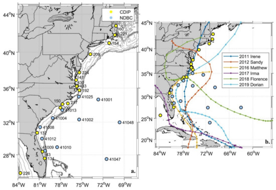
Figure 1.
(a) Map of the Northern Atlantic Ocean showing CDIP and NDBC locations used in the study and (b) buoy location map overlaid with hurricane tracks assessed in this study.
2. Materials and Methods
Hurricane track data were downloaded from the Atlantic hurricane database known as HURDAT2 (https://www.nhc.noaa.gov/data/ (accessed on 20 October 2020)). Track data from individual storms were parsed from the comma-delimited text format publicly available through the National Hurricane Center. The temporal resolution of the track data is six hours and includes location, maximum winds, pressure, and size associated with each storm. The maximum winds at each point were used to classify storm intensity using the Saffir-Simpson Hurricane Wind Scale.
Throughout this study, results are often presented in a storm-centered reference frame where geographic coordinates are transformed to a storm-centered reference frame using the orientation of the storm and the radius of maximum winds (Rm). We follow the work of [13], who proposed 3 azimuthal spatial divisions relative to the direction of the storm’s forward translation at 0°, a left sector (240–20°), a right sector (20–150°), and a back sector (50–240°). The authors separated the three sectors according to their typical wave-directional characteristics: Left: unimodal spectra with peak long-wavelength waves (~300–350 m) moving outward relative to the wind by 60–90°; Right: bimodal or trimodal spectra shifting to longer wavelengths (~200–300 m), outward relative to dominant waves moving outward by up to 45°, relative to the wind direction; Back: unimodal, short-wavelength (~150–200 m) waves moving with the wind. Distances from the storm center are normalized by Rm.
2.1. Buoy Arrays (CDIP/NDBC)
The CDIP at Scripps Institution of Oceanography operates a network of wave monitoring buoys that are composed of moored Datawell WaveriderTM directional wave buoys, positioned along the U.S. East Coast in water depths ranging from 10–30 m. CDIPs fleet of Datawell WaveriderTM buoys are fitted with the HIPPY-40 accelerometer/magnetometer system that measures the displacement path. Averaging intervals of 30 min are used to compute statistical wave parameters, wave energy spectra, and the first four coefficients of the directional spectrum. In-house quality control checks reject observational outliers caused by non-orbital applied accelerations, primarily breaking waves.
The NDBC operates the most extensive wave buoy network in the world with coverage offshore and along most of the U.S. coastline, including Alaska, Hawaii, and the Great Lakes [42]. For this work, we utilize the Atlantic Ocean network providing coverage for North American hurricanes. The NDBC buoy data typically includes hourly measurements of Hs, the 1D energy density spectrum and the cross-spectral moments a1, b1, a2, and b2. Observational buoy networks, such as the NDBC and the CDIP network, have been used for numerous studies, including the historical characterization of deep water and nearshore wave climates [43,44,45], observations within TCs [9,11,16], and prediction of rogue waves [46].
2.2. Numerical Models
Numerically simulating ocean waves during tropical events captures the physical processes of generation, propagation, and dissipation. Modern 3rd generation phase-average wave models (e.g., WAM, WW3, or SWAN) are based on the wave–action equation that balances sources and sinks of wave energy against numerical propagation. The source terms account for how waves grow on the ocean surface, based on surface wind field input (Sin), how energy is transferred from higher wind–wave frequencies to lower swell frequencies through weakly nonlinear wave–wave interactions (Snl), and how wave energy dissipates based on external forces (e.g., bottom friction (Sbot), whitecapping (Swc), depth limited breaking (Sb)). Wave propagation is based on the linear dispersion equation. Each model has its own numerical schemes and source terms to calculate wind–wave interactions and dissipations, but generally each uses the discrete interaction approximation (DIA) to compute wave–wave interaction terms. Each model can be set up with different options that can affect the estimates of wave height from TCs. Additionally, the method used to estimate the input wind speeds for the models can have O(1) effects on the wave estimates. To this end, we have collected four commonly used numerical models and meteorology setups (Table 1) to assess the accuracies and limitations in the prediction of wave energy during TCs. None of the models consider ocean currents.

Table 1.
Formation/dissipation dates, maximum winds and minimum pressures of the six hurricanes assessed in this study.
2.3. WW3 NCEP
The National Oceanic and Atmospheric Administration (NOAA) National Centers for Environmental Prediction (NCEP) WAVEWATCH III (WW3) production hindcast uses two different source term setups. From 2005 to 2015, the model uses the Tolman and Chalikov [47] (ST2) source term package, while from 2015 to 2019 the model uses the ST4 source term package [48]. ST2 and ST4 represent different physical parameterizations of the wind input and whitecapping. The model is set up with rectangular grids using nesting from global 30 arcmin resolution to 4 arcmin resolution at the U.S. East Coast with data outputted at 3-h intervals. The model uses meteorological forcing from the NOAA NCEP Global Forecast System (GFS), which has a native resolution of 30 arcmin and does not include wave–current interactions. Directional wave spectra are outputted at specific buoy locations and were retrieved as monthly ascii spectral bulletins from a public FTP server (https://data.nodc.noaa.gov/thredds/catalog/ncep/nww3/catalog.html (accessed on 25 February 2020)). This hindcast is currently available from Feb 2005 to May 2019. Due to the lag in posting of hindcast results, the operational version of the NCEP WW3 Production Multigrid nowcast model was used for analysis after 2019 August.
2.4. ECMWF ERA5
The European Center for Medium-Range Weather Forecasts (ECMWF) ERA5 hindcast differs from the other models tested because it is a fully coupled climate hindcast [49]. The system passes information from atmospheric models to wave models and gets data back as it marches forward in time. The atmospheric model is also coupled to a data assimilation scheme to improve estimates based on in-situ and remote observations. The wave model used in the ERA5 system is an ECMWF improved version of the WAM model. More specifically, the wave model has updates to the whitecapping, swell dissipation, and wind–wave growth terms based on [50]. The wave model runs on a global 0.36 degree resolution grid. However, access to the directional wave spectra was limited to 0.5 degree output. Gridded bulk wave parameters and spectra were accessed as GRIB files from the Copernicus Climate Data website product: ERA5 hourly data on single levels from 1979 to present [51]. Model parameter values were interpolated at discrete buoy locations from the geographic field grid using a weighted average of nearest output points.
2.5. WW3 IFREMER
The French Research Institute for the Exploitation of the Sea (IFREMER) runs a global hindcast from 1990 to 2019 using WW3 with the ST4 source term. The model uses a nested 10 arcmin grid along the U.S. East Coast within a global 30 arcmin global grid. Meteorological forcing for the model is provided by the ERA5 hindcast product from ECMWF. The wave model is temporally optimized to account for the non-stationarity in the estimation of wind speeds from atmospheric models. We use the 10 arcmin point spectral output product with a 3-h temporal resolution. Data at individual buoy locations were accessed as monthly NetCDF files via the IFREMER FTP server (ftp://ftp.ifremer.fr/ifremer/ww3/HINDCAST/ (accessed on 25 February 2020)).
2.6. USACE WIS
The U.S. Army Corps of Engineers (USACE) Engineer Research and Development Centers (ERDC) Coastal and Hydraulics Laboratory (CHL) produces the Wave Information Study (WIS) hindcast. WIS has been ongoing since the 1970s, providing crucial wave climate information along all the U.S. coast, Great Lakes, and island territories. The WIS East Coast wave hindcast uses the WW3 model with ST4 source term. The model has nested grids from a 0.5-degree grid covering the full Atlantic Ocean down to 5 arcmin for the U.S. East Coast with wind fields produced by Oceanweather Inc (OWI). The background NCEP/NCAR reanalysis [52] wind fields are improved using a combination of statistical downscaling, assimilation of in situ and satellite observations, and dedicated analysis of select tropical and extratropical systems.
A summary of the wave model setups is provided in Table 2. The NCEP, IFREMER, and ECMWF models had a temporal resolution of 3 h. The 0.5 h resolution Hs buoy observations and the 1 h WIS Hs outputs were interpolated to match the 3 h resolution of the other wave models. If wave model point outputs at discrete buoy locations were unavailable, a weighted average of the nearest outputs from the modeled 2D geographic grid was used.
Table 2.
Summary of numerical wave model setups used for this study.
3. Buoy-Model Comparisons
As part of the hindcast performance assessments, significant wave heights (Hs) were computed from the zero-order moment of the one-dimensional (1D) wave energy spectrum (E(f)),
where and f is frequency. Model and buoy Hs was used to compute Hs bias (i.e., mean percent error):
where n is the total number of model output—buoy observation pairs. In addition, standard error statistics of root-mean-square-error (rmse) and correlation coefficient (cc) were computed. For this assessment, we defined a hurricane signature as a substantial deviation from ambient wave conditions with a minimum Hs criterion of 3 m.
3.1. Buoy-Model Hs Bias
A comparison of all hurricane signatures from the six hurricanes assessed in this study to co-located model outputs showed a consistent negative model bias (i.e., Hs underestimation) across the array of operational buoys. Buoy-model Hs scatter plots indicated the bulk of the model outputs compared well to observations, but as wave heights increase, so did model differences as evident by the larger spread around the 1:1 line, with an overall negative bias of −7.1%, −6.7%, −2.7%, and −2.3% for the NCEP, IFREMER, ECMWF, and WIS models, respectively (Figure 2).
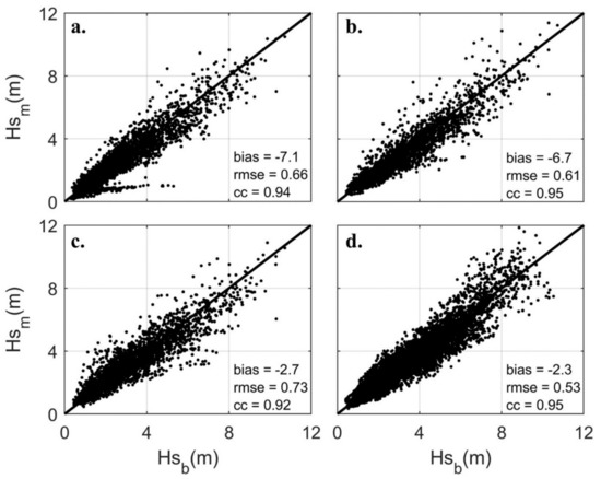
Figure 2.
Buoy-model Hs comparison plots for (a) NCEP, (b) IFREMER, (c) ECMWF and (d) WIS wave models for all six hurricanes at all buoy locations. (a–c) Wave models have a 3-h temporal resolution; (d) 1-h temporal resolution. Error statistics for each model is provided in each figure.
3.2. Buoy-Model Wind Comparisons
More accurate representations of the surface wind field have been a key element in the improvement of model wave results. However, the common assumption that wind field inaccuracies are the primary source of wave modeling errors during TCs is being disproved due to recent advancements in meteorological modeling, driven by increased computing power and a growing database of satellite data [35]. NDBC buoy-model wind comparisons were used to determine if systematic trends persist that may explain the general pattern of model Hs underestimation evident in Figure 2. The minimum wind velocity for classification of a gale force wind of 14 m/s, as defined by the Beaufort scale, was used as a minimum threshold for the comparisons. The results showed modeled winds tended to overestimate observed NDBC winds during the six hurricanes (Figure 3), except for the ECMWF ERA5 wind field. NCEP, IFREMER, and WIS comparisons had overall positive biases of 5.4%, 3.9%, and 6.3% respectively. The results suggested wind input was not the primary source of model Hs underestimation errors, in agreement with previous studies [35].
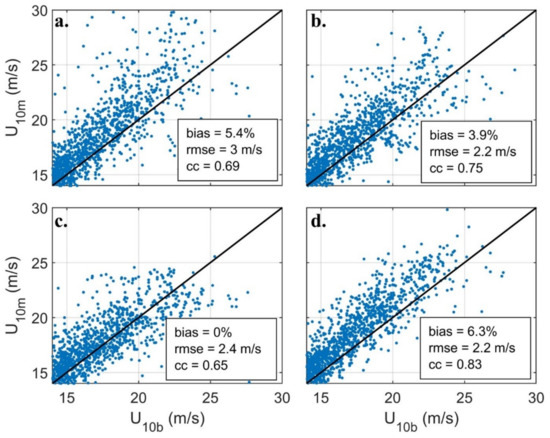
Figure 3.
Buoy (U10b)-model (U10m) wind comparison plots for (a) NCEP, (b) IFREMER, (c) ECMWF and (d) WIS wave models for all six hurricanes. Error statistics for each model is provided in each figure.
3.3. Hs Bias Depth Dependency
The observed dominant periods of the storms assessed in this study ranged from around 13–16 s (s), corresponding to an approximate wavelength range of 264–400 m. Linear wave theory estimates the longest period waves (16 s) will begin to feel the bottom at a depth approximately one-half the wavelength (~200 m), resulting in swell that was impacted by intermediate water physics (e.g., bottom friction, refraction, shoaling) across the continental shelf of the U.S. East Coast (Figure 1a). The transition from an intermediate wave region over the shelf to a shallow water wave region occurs at approximately 1/20 of the wavelength or 20 m for a 16 s swell.
Buoy-model wave comparisons are expected to degrade towards the coast where topographic effects and shallow water physics become increasingly important. Additionally, modeled bathymetry is often too coarse to resolve features that influence wave transformation. As a result, these regions are more difficult to simulate or in some cases are not represented in the model (e.g., diffraction) [53]. To assess the bias variability in extreme wave heights (Hs > 3 m) as a function of depth, cumulative buoy error statistics were computed for binned depth ranges beginning at the shallowest buoy depth and extending to a depth of 50 m (Figure 4). The results showed a generally decreasing performance of models with shallowing depth, with substantial degradation of correlation near 20 m depth where the largest swell transitions to shallow water waves. The wave models have a cc around 0.9 at the 23.5 m depth bin that degrades to a range of 0.3–0.57 at the shallowest bin. Therefore, we used the 20 m depth as a demarcation of “shallow” and “deep” buoys. This threshold provided approximately 60 (shallow) and 150 (deep) total comparison buoys for the six hurricanes assessed in this study (Figure 4d).
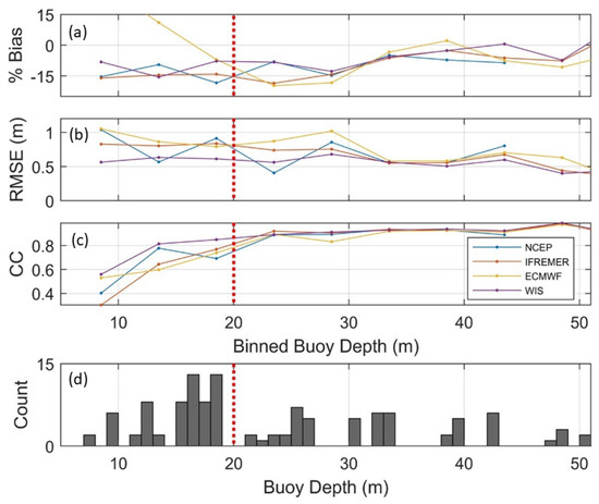
Figure 4.
Buoy-model (a) percent bias, (b) rmse, and (c) cc error statistics for observed Hs > 3 m for all six hurricanes computed at 5 m depth increments using all buoy-model comparisons within each bin. (d) Histogram of buoy depths. The dotted red line denotes demarcation between “shallow” and “deep” buoy depths chosen for this study.
Scatter plots of Hs bias at deep locations showed a relatively well-behaved relationship around the 1:1 line that increased in variability for larger wave heights, with a tendency for model Hs to slightly underestimate observed Hs. Conversely, substantial variability was evident between comparisons at shallow buoy locations that resulted in larger Hs differences. These large error discrepancies between deep and shallow model performance are illustrated for the NCEP comparisons (Figure 5a,b). The buoy to NCEP model comparisons revealed a few times when the NCEP model failed to simulate the hurricane energy at shallower depths. This was evident during periods when simulated Hs remained small and relatively constant compared to increasing Hs observations that resulted in outliers extending from the 1:1 line (Figure 5b).
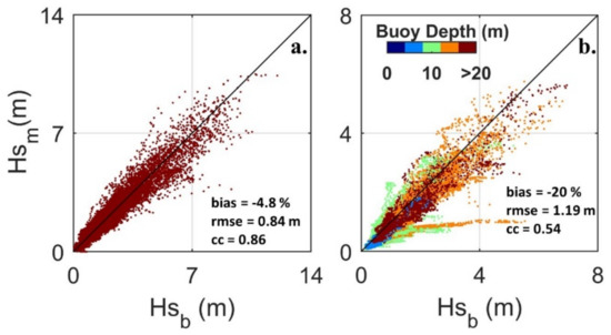
Figure 5.
Comparison plots of buoy significant wave height (Hsb) to NCEP simulated significant wave heights (Hsm) for (a) buoy depths greater than 20 m and (b) less than 20 m. Error metrics were provided for each plot for Hs > 3 m.
The initial bias comparisons for all six hurricanes indicated wave models generally underestimated hurricane generated waves. Increased discrepancies in shallow water were evident where shoaling, refraction and dissipation become important mechanisms in wave transformation across the shelf. In deeper waters, buoy-model Hs comparisons yielded similar overall statistics for the NCEP, IFREMER, ECMWF, and WIS hindcasts, with underestimation in simulated Hs typically in the −5% to −9% range. However, substantial variability in the error statistics was apparent across all models for shallow buoys locations (Table 3). The NCEP and WIS models had the highest coastal grid resolutions of 4 arcmin and 5 arcmin respectively of the four models. Yet, the NCEP model performance was worse than the other models while the WIS model performed well, with lower rmse and higher cc than the other wave models. The 10 arcmin IFREMER product performed slightly better than NCEP with improved rmse, cc, and a bias of −16.1% compared to the NCEP bias of −20%. The lowest coastal resolution (21 arcmin) ECMWF product exhibited the lowest cc (0.49) suggesting insufficient model resolution to properly simulate the coastal wave field during TCs. Additionally, the temporal resolution of the wind fields (3 h) may not have captured the local temporal variability in coastal regions.
Table 3.
Summary of error statistics for deep (>20 m) and shallow (<20m) buoy locations for four hindcast wave models. Statistics were computed from all observed extreme wave events (Hs > 3 m) generated from the six hurricanes.
4. Case Studies
Cumulative statistics for the six hurricanes assessed in this study showed wave models generally underestimated extreme waves generated by TCs with larger errors observed at shallower depths (Table 3). However, aggregating data masks error patterns unique to each model and storm suggesting analysis on a per storm basis is the preferred approach for a limited number of TCs. Therefore, detailed buoy-model assessments were made for Sandy and Florence, two storms that had notable differences in size, intensity, storm track, and speed.
While translating northeast (NE) along the U.S. East Coast, Hurricane Sandy became the largest Atlantic hurricane on record (spatially). At its maximum size, its tropical-storm-force winds spanned approximately 1850 km with Rm over 200 km. As a result, the TC impacted the entire U.S. East Coast buoy array with observed waves approaching 12 m at several NDBC buoy locations (Figure 6a). Conversely, Florence was a powerful, compact TC, with a unique east to west approach to the U.S. East Coast (Figure 6b). Sandy rapidly intensified to a category 4 near buoy 41049 with a small, but intense Rm around 30 km. The storm sustained its energy until passing buoy 41048 where it began to slowly weaken as it approached land. The NDBC/CDIP buoy array was well positioned to assess hindcast wave model performance during these two distinct extreme events.
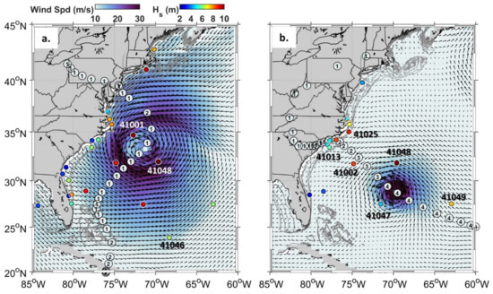
Figure 6.
Map of NCEP 30 arcmin global wind product for Hurricanes (a) Sandy at 20:30 UTC on 2012 October 28 and (b) Florence at 09:00 UTC on 2018 September 12. Each figure was overlaid with the modeled wind vectors (black arrows) for each storm. The blue-white color scale represents the intensity of the wind. The color scale provided at each buoy location denotes the maximum observed Hs during the storm at that buoy location. TC track bubbles contain storm category (Saffir-Simpson scale) at that location.
4.1. Case Study: Hurricane Sandy
The large Rm during Sandy resulted in extreme waves across most of the U.S. East Coast buoy array that allowed bias patterns to be assessed in the TCs wave field (Figure 6a and Figure 7). A limitation of previous comparisons was the lack of spatial and temporal information about model biases with respect to a TCs position. To assess spatial variability in model error, buoy and model geographic coordinates were transformed to a storm-centric frame of reference separated into three sectors, left, right, and back. Similar to previous studies [18,19], wave assessments for this work were primarily limited to the region less than eight times the radius of maximum winds (Rm) (Figure 7, dotted circle), where wave development is typically fetch-limited and the spectra typically unimodal. A summary of all hurricane Hs observations from this study relative to storm position showed the expected trend of increasing Hs nearer the hurricane eye. The largest waves occurred in the right sector where waves were forced under extended fetch conditions. (see Supplementary Figure S1).
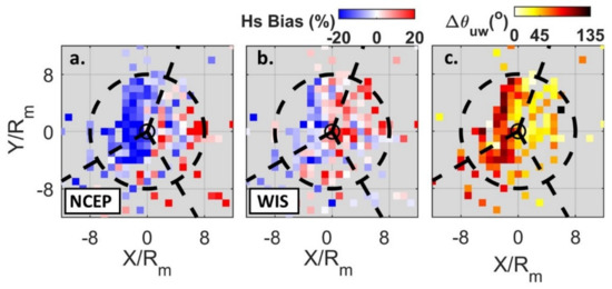
Figure 7.
Hs bias at all buoy locations during Hurricane Sandy for (a) NCEP and (b) WIS in a storm-centric frame of reference with distance from the eye normalized by the radius of maximum winds (Rm). (c) Difference between dominant wave direction and wind direction (). Observations were binned into 1 Rm × 1 Rm bins. The inner circle denotes 1 Rm and outer dotted circle denotes 8 Rm. Direction of storm motion is up the page.
The most prominent pattern from these assessments was evident for the NCEP and WIS models that consistently overestimated Hs in the right sector and underestimated Hs in the left and back sectors (Figure 7a,b). NCEP comparisons exhibited larger underestimation in the left sector while more prominent overestimates were observed for WIS comparisons in the right sector. Specifically, the NCEP model had biases of −16.8%/4% (left/right sectors), compared to −3.8%/6.2% for the WIS model. The IFREMER results were similar, but the model overestimates in the right sector were confined to the upper right region of the storm (Figure S2). In comparison to the variability in Hs biases found in WW3 models, the WAM ECMWF model exhibited consistent underestimation of Hs in all sectors.
The pattern seen in NCEP and WIS, underestimates/overestimates on the left/right side of hurricane Sandy, contrasted what was found during Hurricane Ivan [15]. The authors found WW3 models tended to overestimate the wave energy on the left side of the storm where winds were generally oblique with respect to the wave propagation direction. To look for correlation between Hs bias patterns and wind–wave alignment, we defined the angle between wind direction and the peak wave direction as . Following [14,15,54], we separated observed wave conditions as wind sea or following swell (WS/FS) when ≤ 45°, cross swell (CS) when 45° < ≤ 135° and opposing swell (OS) when > 135°. In the near-field (near 1 Rm) waves were typically dominated by cross-swell (CS) in the left sector, following-swell (FS) in the right sector, and opposing-swell (OS) in the back sector. Plotting in a storm-centric frame of reference revealed the expected near-field patterns extended away from the center of the storm in both the left and right sectors, possibly due to Hurricane Sandy’s size (Figure 7c). WS/FS or wind–wave directions approaching WS/FS were primarily observed on the right side of the storm where overestimates in modeled wave energy occurred for the NCEP and WIS outputs. CS conditions were prevalent on the left side of the storm. The observations from the shallower NDBC buoys 41012 and 41013 (Figure 6a) exhibited the largest wind–wave direction differences due to waves refracting to angles approximately parallel to bathymetry contours. WIS compared relatively well in this region with a slight negative bias in contrast to the substantial underestimates that were evident for NCEP, IFREMER, and ECMWF comparisons (Figure 7a,b and Supplementary Figure S2).
Observations from three NDBC buoys (41046, 41047, 41048) accounted for all deep-water Hs bias comparisons in the right sector of Hurricane Sandy. Buoys 41046 and 41048 were used to assess NCEP/WIS overestimation errors on the right side of the storm with respect to the TCs characteristics (e.g., size, Rm, location, storm track).
Buoy 41046 was located approximately 700 km to the northeast of the storm track when Sandy transitioned to a northwesterly (NW) direction on 25 October 2012 with a small Rm around 35 km. Along this track, the Rm grew to 110 km on 27 October prior to another shift in direction to the NE (parallel to the coast). The building seas during this period were well captured by the WIS wave model yet missed by the NCEP and ECMWF outputs (Figure 8a and Figure 9a). The differences appeared to result largely from overestimated wind input during a period that would have otherwise caused little wave growth to be simulated at 41046 (Figure 8b). The growing Rm and the storm’s interaction with land during this timeframe suggest topographic effects likely influenced NCEP and ECMWF simulations. The resulting buoy–model (NCEP/WIS) Hs bias spatial patterns were illustrated in Figure 10a,b. NCEP winds during this time showed similar tendencies as Hs, with large overestimates in comparison to observed winds at 41046 (Figure 8b). As the storm track changed to the NE, the initial sea state generated by the previous NW track waned and was overestimated by both the NCEP and WIS models (Figure 8a), resulting in regions of large positive biases directly east of the hurricanes center at a distance around 7 to 8 Rm (Figure 10a,b). As the storm propagated up the coast, the Rm expanded to a peak size of ~ 220 km on 29 October before shifting again to the NW for its final landward approach. The increasing size of the hurricane resulted in observations at buoy 41046 that remained within 8 Rm even though the buoy was over 1000 km away from the storms center. The change in direction and subsequent move parallel to the coast over the course of around 2 days resulted in a secondary hurricane signature at 41046 (primarily located in the back sector) that was well captured by the WIS model except for underestimation of the observed dual Hs peaks (Figure 8a). The NCEP underestimated the second wave field, similar to IFREMER and ECMWF comparisons (Figure 8a). None of the four models replicated the low frequency bi-modal wave spectra observed at t2 (Figure 9b).
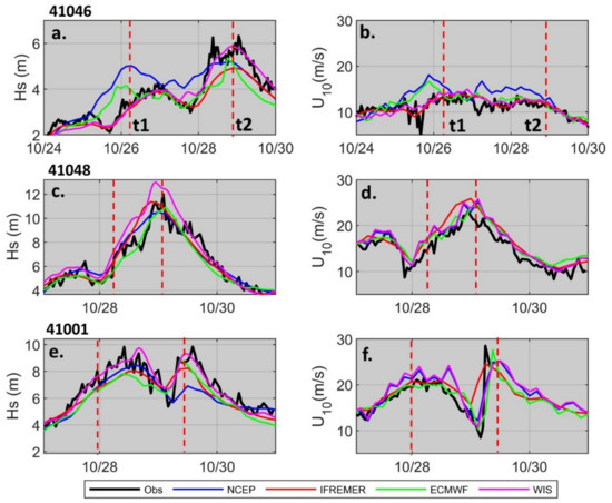
Figure 8.
Buoy-model time-series comparisons of (a,c,e) Hs and (b,d,f) model wind input for buoys (a,b) 41046, (c,d) 41048, (e,f) 41001 during Hurricane Sandy. Red dotted vertical lines denote the times used to assess the 1D wave spectra in Figure 9 (t1, t2).
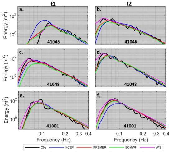
Figure 9.
Buoy-model 1D wave spectra comparisons at (a,c,e) t1 and (b,d,f) t2 (see Figure 8) for buoys (a,b) 41046, (c,d) 41048, (e,f) 41001 during Hurricane Sandy.
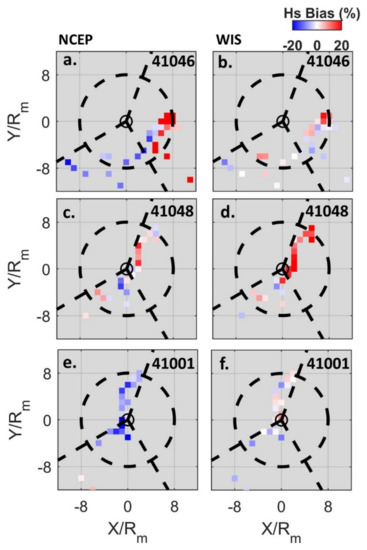
Figure 10.
(a,c,e) NCEP and (b,d,f) WIS Hs biases at buoys (a,b) 41046, (c,d) 41048, (e,f) 41001 during Hurricane Sandy. Plots are in a storm-centric frame of reference with distance from the eye normalized by the radius of maximum winds (Rm). Observations were binned into 1 Rm × 1 Rm bins. The inner circle denotes 1 Rm and outer dotted circle denotes 8 Rm. Direction of storm motion is up the page.
During the time between the two hurricane signatures at 41046, wave energy decreased due to a storm track shift to the NW. Large Hs overestimates in NCEP (Figure 8a) were evident during this period, but do not correlate with biases in wind inputs from buoys along the hurricane track (e.g., 41010). Similarly, a large NCEP Hs bias at 41001, after the hurricane track shifted to its final landward trajectory, did not appear to be caused by inadequate wind forcing. The model underestimation of the second Hs peak (Figure 8e) was larger for the NCEP model than the other wave models despite having similar winds (Figure 8f), thus suggesting a different source of error.
The Rm of Hurricane Sandy as it approached NDBC buoy 41048 was 220 km, approximately the same distance of the buoy to the TCs center at its closest. The exposure to extended fetch and maximum winds in its right front quadrant location resulted in the largest Hs (~12 m) observed across the buoy array (Figure 6a and Figure 8c). Buoy-model winds at 41048 compared relatively well, with overestimates observed near the Hs peak for NCEP, IFREMER, and WIS hindcasts (Figure 8d). The wave field at 41048 began to build after Sandy’s track shifted to the NE at a distance of ~8 Rm (Figure 10c). NCEP showed patterns of increasing overestimation in Hs as the storm approached the buoy, transitioning to underestimation at the observed Hs peak. The underestimation persisted as the storm shifted to its final NW trajectory. The WIS comparisons showed more overestimates in the right sector (i.e., preceding and during peak Hs) before better performance was evident in the back sector as the TC approached the coast (Figure 10d). The evolving 1D spectra at 41048 was highly variable. This resulted in irregular buoy-model differences as the storm approached. At t1, was approximately 70°, resulting in a bi-modal 1D spectra that was not simulated well by the wave models (Figure 9c). The observed peak period of 14 s was underestimated by NCEP simulations (~12 s). Starting around six hours after t1, models consistently overestimated Hs prior to peak Hs values. The higher resolution WIS outputs consistently overestimated energy in the low frequency region prior to the spectral peak (Figure 9c,d), contributing to consistent overestimation of Hs in the right sector of Hurricane Sandy (Figure 8c and Figure 10d). The IFREMER Hs bias pattern was similar to the NCEP model. Conversely, ECMWF Hs compared well in the right sector with larger underestimation evident in the back sector (Figure 8c and Supplementary Figure S2).
Comparisons at 41046 and 41048 provided examples of model Hs overestimation errors in the right sector of Hurricane Sandy. The NDBC buoy 41001 was used to provide a contrasting example of typical underestimation patterns observed at buoys located on the left side of the TC. It was a similar distance from the eye of Hurricane Sandy as 41048, but on the weaker left side of the storm (Figure 6a). WIS Hs outputs at 41001 compared well to observed wave heights (Figure 8e and Figure 10f). Conversely, NCEP outputs revealed a tendency of Hs underestimation, with a large underestimation of the wave energy after the storm track changed to its final NW direction generating a second Hs peak (Figure 8e, Figure 9f and Figure 10e). The NCEP Hs underestimation pattern observed in the left sector for 41001 was in contrast to an overestimation pattern evident at 41048, located in the right sector of the storm. Both IFREMER and ECMWF models also tended to underestimate both Hs peaks (Figure S3).
4.2. Case Study: Hurricane Florence
In addition to a unique perpendicular shoreline approach, Hurricane Florence had the smallest Rm of the storms assessed in this study, generating a compact, spatially and temporally variable wave field. The small size of the storm resulted in a limited spatial distribution of observations from buoys along Florence’s storm track (Figure 11). A pattern of Hs overestimation on the left side and underestimation on the right side of the storm was observed across the four wave models with substantial model underestimates near the eye from direct or near-direct hits on the shallower buoys as Florence made landfall (Figure 11a,b). The overestimation pattern in the CS region (left side) and underestimation in the WS/FS region (Figure 11c) of the storm was in contrast to the results found for Hurricane Sandy. An exception to this pattern was buoy 41025 located on the right side of the storm that showed a consistent positive Hs bias as the storm passed (Figure 11a,b). While the general Hs bias patterns for each wave model was similar, the high spatial and temporal variability of the compact storm resulted in varying responses between the different models.
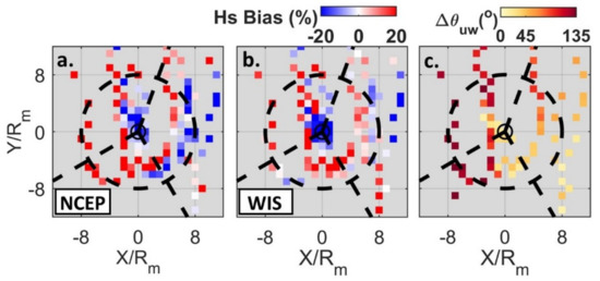
Figure 11.
Hs bias at all buoy locations during Hurricane Florence for (a) NCEP and (b) WIS in a storm-centric frame of reference with distance from the eye normalized by the radius of maximum winds (Rm). (c) Difference between dominant wave direction and wind direction (). Observations were binned into 1 Rm × 1 Rm bins. The inner circle denotes 1 Rm and outer dotted circle denotes 8 Rm. Direction of storm motion is up the page.
To further assess wave model performance during Hurricane Florence, Hs, wind speed, and 1D spectra comparisons were made to several buoy observations located on either side of the storm track (left: 41049, 41048, 41025; right: 41047, 41002, 41013) (Figure 6b). Hurricane Florence underwent rapid intensification (RI) to a Category 4 storm as it approached buoy 41049, reaching its peak intensity around 1800 UTC 11 September, approximately 9 h after transiting past the buoy. At its closest, the TC was 170 km from the buoy with a small Rm of 27 km that resulted in a large gradient in wind speeds from the eye to the buoy that was not well captured by the wind inputs for the NCEP, IFREMER, and ECMWF wave models (Figure 12a). Regardless of overestimated winds, only the NCEP wave field showed consistent overestimation in Hs while WIS (best wind comparison) underestimated Hs as the storm passed (Figure 13a). The TC next passed nearly equidistant between buoys 41047 (left) and 41048 (right), where large modeled Hs overestimation and underestimation was evident, respectively. The modeled winds at 41047 compared well to the observed smaller winds, but a large underestimation of peak winds was evident at 41048 (Figure 12c). Hs comparisons at these two locations resulted in the largest differences in bias out of six buoys assessed. Hs overestimates were evident of ~20% to 30% (except for ECMWF) at 41047 and underestimates of 3 to 4 m (~27% to 36%) for all models at 41048 (Figure 13b,c). The underestimation of Hs at 41048 began prior to the underestimation of wind, suggesting wind alone was not the primary mechanism affecting model performance. Conversely, improper wind input was a primary mechanism for large buoy-model Hs errors at 41002. The buoys distance to the storm (~2.5 Rm) subjected it to the higher gradient winds nearer the center of the TC that were not well represented in the hindcast models, likely contributing to the large buoy-model Hs errors (Figure 12d and Figure 13d).
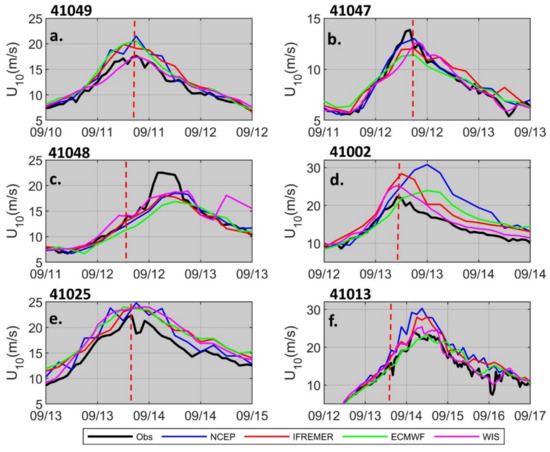
Figure 12.
Buoy-model time-series comparisons of model wind input for buoys (a) 41049, (b) 41047, (c) 41048, (d) 41002, (e) 41025 and (f) 41013 during Hurricane Florence. The red dotted vertical line denotes the time used to assess the 1D wave spectra in Figure 14.
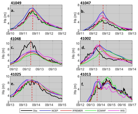
Figure 13.
Buoy-model time-series comparisons of Hs for buoys (a) 41049, (b) 41047, (c) 41048, (d) 41002, (e) 41025 and (f) 41013 during Hurricane Florence. The red dotted vertical line denotes the time used to assess the 1D wave spectra in Figure 14.
Two additional buoys impacted by the TC were 41025/41013, located on the right/left side of the TC, and at depths of 60 m and 33 m respectively. At both locations, model wind inputs were overestimated with increasing differences near the peak, except for the ECMWF winds at 41025 (Figure 12e,f). While buoy-model Hs compared relatively well at 41025, more variability was observed between the models at 41013. The Hs comparisons were unique due to an easterly shift in storm track and a decrease of the TCs translation velocity to ~2.5 m/s as it approached the coast, as evident by the extended time span of high waves (Figure 13f). The initial wave field was overestimated by NCEP and WIS models while IFREMER performed better. The ECMWF model lagged the observed peak and also overestimated peak Hs. The subsequent wave field generated after the change in track direction and slowing of the storm was well captured by the IFREMER model, with Hs overestimates and underestimates evident around the Hs peak for the ECMWF and NCEP models, respectively. The WIS model underestimated the wave energy at this location as the storm approached the coast (Figure 13f).
Separating buoy-model comparisons by location based on Hurricane Florence’s storm track (i.e., left/right) revealed several general patterns. Comparisons showed model resolutions were not able to replicate the higher frequency fluctuations in the Hs observations. As the buoy approached the coast, three distinct Hs peaks were evident (each with decreasing peak period) in each of the buoy wave records located on the right side of the storm, (Figure 13a,c,e). At 41048, the peak period decreased from 15.4 s for the first peak to 13.8 s, and 12.1 s for the two subsequent peaks, with peak directions increasing from 134°, to 149°, and 159° respectively. Peak 1 in the Hs wave record were the fastest waves (15.4 s), followed around 6 h later by a wave field with peak periods of 13.8 s, followed around 3 h later by the slower 12.1 s waves, all coming from increasingly larger angles. This was consistent with the dispersion of different swell waves generated along the right side of the storm toward buoy 41048 as the hurricane passed [9,11]. These complex variabilities in the wave fields were not resolved by the 3-h temporal resolution of the NCEP, IFREMER, and ECMWF models. The higher resolution WIS (1-h) model also did not resolve these features (Figure 13a,c,e), suggesting there were other processes modulating the Hs time series, e.g., water-level and wave–current interaction.
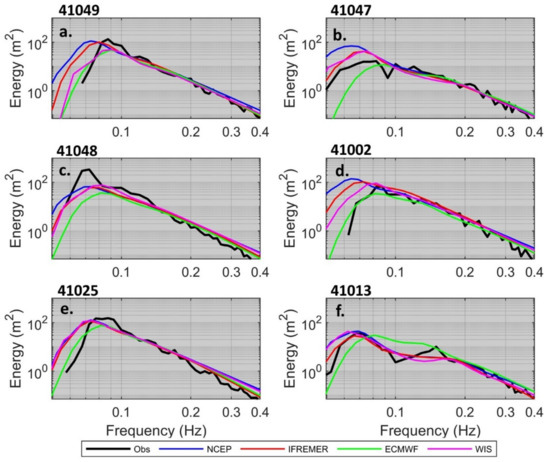
The 1D wave spectra comparisons (red dotted lines in Figure 13) illustrated common mismatches in the wave energy–frequency space for wave fields generated by Hurricane Florence. In the RI region observed at 41049, the NCEP and IFREMER wave energy outputs missed the frequency of the observed peak resulting in overestimates in wave energy at low frequencies (Figure 14a). A higher peak frequency at 41049 (0.09 Hz) was evident in comparison to an observed peak frequency of 0.07 Hz at 41048, consistent with a region undergoing RI that continues to strengthen into the wave fields observed at 41048. The 1D wave spectra comparisons suggest the NCEP and IFREMER models were not accurately simulating the wave growth at 41049 (Figure 14a). Similar low frequency errors were evident in the 1D wave spectra comparisons at 41002 (Figure 14d). where temporal differences exist between observed and modeled Hs peaks (Figure 13d). At 41048, the peak wave energy at low frequencies was missed by each wave model, while on the opposite side of the storm at 41047, the low frequency peak energy was substantially less and overestimated by all models except the ECMWF (Figure 14b). The two shallower buoys (41025 and 41013) observed wave fields generated while the TC was weakening and slowing down. The 1D spectra at 41025 showed higher frequency (i.e., lower swell period) swell energy (Figure 14e) than what was observed at 41048 (Figure 14c). In addition to the strength and speed of the storm, the energy at 41025 was also likely being dissipated as it increasingly felt the bottom across the continental shelf. The models consistently had peak swell energy at lower frequencies than observed, resulting in Hs overestimates. The high frequency tail of the spectra at 41025 was also generally overestimated by the models and could have contributed to the observed Hs overestimation (Figure 14e). The final wave spectra example taken at the Hs peak prior to Florence’s direction change and slow, landward approach, illustrated a bi-modal spectra that was overestimated at low frequencies and underestimated at the higher wind wave frequency (Figure 14f). The ECMWF model performed worst, likely due to its lower resolution in comparison to other wave models assessed in this study. In the CS region of the hurricane, bi-modal peaks were common during building seas (i.e., preceding Hs peak region) and exhibited similar patterns with models typically missing the secondary wind peak.
4.3. Mechanisms of Buoy-Model Differences
Our analysis of all six hurricanes showed an overall Hs underestimation pattern that was exacerbated by shallow water. However, this broad-stroke approach masks error patterns unique to each storm as shown for two case studies, hurricanes Sandy and Florence. The results suggested there were likely multiple sources of wave model errors that vary dependent on model used and hurricane attributes (e.g., size, speed, intensity, geographic location). The complex confluence of multiple error sources, especially in shallow water, made it difficult to tell a simple story about why models were in error. However, we can highlight common errors observed and speculate on possible causes based on our results and previous literature.
A major difference between NCEP and the other hindcast models for Hurricane Sandy was NCEP used the ST2 source term package instead of ST4 used by the other models. A review of the literature showed varying performance results for ST2 under strong storm conditions. Studies by [55,56] showed that the ST2 physics was the best option during TCs over other source term packages in the Indian Seas and in shallower waters (<100 m) around Zhoushan Islands in the South China Sea. Conversely, [15] found ST2 parameterization to be the least accurate (in comparison to ST3, ST4, and ST6) with a systematic underestimation of waves larger than 6 m during Hurricane Ivan. They concluded that the ST2 cap of the drag coefficient (Cd) that becomes active well below hurricane wind forcing likely explained underestimation of high waves. Our results show larger underestimates of Hs along the left side of Sandy (when compared to other WW3 models) with more occurrences of Hs overestimates in the right sector as discussed previously (Figure 7a). If indeed the upper limit cutoff of Cd was contributing to NCEP Hs underestimations, the examples of overestimation hint at additional issues during the wind–wave growth phase after a TC makes a substantial course change. However, the TC climatological study by [57] compared IFREMER hindcasts (1990–2016) to altimeter observations and found overestimation on the right side of TCs. This suggests the WW3 Hs overestimation observed on the right side of Hurricane Sandy could be a more systematic wave-growth issue instead of outliers due to Sandy’s course changes.
The discrete interactive approximation (DIA) approach used by operational wave models to compute the nonlinear four-wave interactions have known issues under TC conditions. [32] found large Hs overestimates (up to ~20%) in all sectors of an idealized hurricane with Rm of 50 km. Yet, a trend of Hs overestimate/underestimate in the left/right side of the hurricane was evident for default DIA-WW3 runs, opposite of that seen for Hurricane Sandy [58]. Another limitation of the DIA method is that it is known to produce an overly broad frequency spectra [15,59] that would smooth bi-modal features observed in our assessment (e.g., Figure 9e and Figure 14f).
Another limitation of operational wave models is that they do not include wave–current interactions. It is well established that large horizontal gradients of ocean currents may significantly affect the surface wave properties [47,60]. Since TC forcing results in strong surface currents with large horizontal gradients, wave–current interactions can be important processes during TCs. Following currents can lead to lengthening of surface waves while opposing currents steepen waves, enhance breaking, and increase dissipation. Ref. [60] used a coupled wind-current-wave model under idealized TC conditions to assess the effects of TC generated currents on the wave field. They found the wave field was significantly affected by the wind–wave current interactions in the region where currents were roughly aligned with the wave propagation direction (e.g., right front sector). The advection effects of currents can introduce Hs overestimates of around 20% and also shift peak frequency to a higher frequency. Similarly, [61] found substantial differences in the Hs wave field dependent on TC translation speeds and the inclusion of wave–current interactions. Therefore, the lack of wave–current interactions could partly explain the overestimation Hs bias pattern seen for NCEP, IFREMER, and WIS results. In particular, IFREMER showed an Hs overestimation pattern that was limited to the upper right sector of Hurricane Sandy (Supplementary Figure S2). However, a more recent study by [62] suggested the modulation of the TC wave field is dominated by background currents in the far-field, not TC induced surface currents. This is particularly true if the TC generated wave-field interacts with strong current regimes such as the Gulf Stream [63,64]. It is likely both TC induced, and background surface currents are important mechanisms modulating the wave field. We see evidence of the former as Hurricane Sandy approached the coastline on the 29 October 2012 generating observed coastal surface currents over 2 m/s offshore of New Jersey to North Carolina [65]. The absence of wave–current interactions likely contributed to some of the largest Hs bias observed during this study at CDIP buoys 147 and 430 with underestimates in Hs ranging from 33% to 45% for all wave models.
Model resolution was also a likely problem area, particularly for the high gradient regions generated by Hurricane Florence. For example, the wave models did not properly reproduce the wave spectra during periods of RI, with consistent overestimates of the low frequency portion of the spectra for NCEP and IFREMER models and underestimates of the spectral peak by ECMWF and WIS models (Figure 14a). The variability in error across the models show properly simulating wave growth during RI remains a challenge. In addition, the tendency of the models to underestimate/overestimate wave regimes on the right/left sides of Florence was similar to error patterns discussed by [32] generated from DIA parameterization errors. However, given the location of 41047 in the CS and near OS region of the hurricane (left, back sectors), another potential source of Hs model error was the wind-induced swell decay (negative wind input), which has been found to be too weak resulting in overestimation errors as discussed by [15]. Ref. [15] showed that enhancing the negative wind input properly can effectively improve model skill in these cases. The low frequency energy in the 1D wave spectra at 41047 contains less energy and looked flat compared to other buoys, consistent with the occurrence of higher swell decay that was not be simulated by the wave models (Figure 14b).
Model Hs errors evident at 41048 and 41002 hints at another issue in simulating small TCs. The companion paper to this work [57] used 26 years of IFREMER output and altimeter data to build composite maps of Hs bias around TCs. The study found that wave model hindcasts consistently underestimated the eye region of TCs, and this underestimation increased in magnitude with small TCs. For some storms, the Rm was smaller than the grid resolution, and errors were clearly related to not capturing the spatial gradients. Similarly, during Florence, the Rm was ~30 km when the hurricane passed 41048 and 41002. Thus, a 30 arcmin model grid resolution (approximately 55.5 km × 55.5 km) would not adequately capture the strong storm gradients. At 41048, the peak winds were not simulated well by the wave models (Figure 12c) contributing to the observed large Hs underestimation up to 3 m at the peak (Figure 13c).
Another interesting error pattern was observed at buoy 41025 that was located in the Outer Banks region in the vicinity of the Gulf Stream (Figure 6a). The models compared better than comparisons at 41048, possibly due to the TCs slowing translation speed and weakening from a category 4 to a category 2 hurricane as it approached the coast. However, the better comparisons could also in part result from the omission of wave–current interactions in operational hindcast wave models. [66] found that the current-induced wave refraction due to strong current shear from the Gulf Stream could induce considerable variation in wave heights. At 41025, peak wave directions varied from 140° to 170°, interacting at an angle with the NW propagating Gulf Stream that would elongate the waves and reduce observed wave heights, thus causing better model comparisons at 41025 than 41048. In addition, a shift to a higher frequency peak (~0.09 Hz) was evident (compared to 0.07 Hz at 41048), also suggesting that wave–current interactions affected the spectral shape of the wave field [60].
As hurricane-induced waves propagate into progressively shallower water, the wave fields become more complex as waves refract, shoal, and dissipate due to coastal topography and bathymetry. Compared to our deep-water assessments, accuracy of wave hindcast models diminish in shallow waters. Wave model assessments for all six hurricanes revealed more variability and decreasing performance in the 20–30-m depth range (Figure 3). Ref. [67] found that longer wavelength, hurricane-induced waves largely dissipate through shoaling-related breaking in this region they termed the “shelf shoulder.” Therefore, it was unsurprising that wave models performed poorer in shallow waters given the additional processes that become important and were not well captured by hindcast setups. Yet, a surprising result of our study was the relatively good performance of the WIS model in simulating Hs in shallow water under TC conditions. With a bias of 12.4%, a rmse of 0.83 m, and a cc of 0.77, the WIS model hindcasts substantially outperforms the other wave models in shallow waters. It was evident from our analysis that the lower coastal resolutions of 10 arcmin and 21 arcmin for IFREMER and ECMWF models, respectively, are not ideal for extreme coastal wave assessments. The NCEP model has a slightly higher coastal resolution (4 arcmin) than WIS (5 arcmin) yet performed poorly in shallow waters in comparison to all other wave models. However, a large portion of the error was from hurricanes Irene (2011) and Sandy (2014) when available NCEP hindcasts used the ST2 parameterization. There was notable improvement in the error metrics for the four storms after the ST4 implementation with a bias of −13.3%, rmse of 0.84 m, and cc of 0.68. These results are more comparable to the WIS performance and suggest both models could be used for TC coastal studies dependent on accuracy requirements.
5. Conclusions
The spatiotemporal variability of intense wind fields from TCs generate complex wave fields that remain difficult to simulate (forecast/hindcast). We find this to be true of the operational hindcast products analyzed here. We compared hurricane signatures (time series at a single location), as observed in the Hs historical records, across the North Atlantic NDBC/CDIP buoy array for six recent hurricanes (2011–2019). These storms were chosen because they were landfalling TCs that impacted the U.S. East Coast. Like previous studies, the numerical hindcast wave models used in this assessment showed a general tendency to underestimate peak significant wave heights, but generally performed well in deep waters. However, a composite analysis of relatively few TCs masks complex Hs bias patterns unique to each storm. Two hurricanes, Sandy and Florence, with notable differences in size, intensity, and track were used to illustrate error patterns distinct to each storm in a storm-centric frame of reference. Contrasting Hs bias patterns were observed between Sandy and Florence with WW3 models exhibiting a tendency to underestimate/overestimate Hs on the left/right side of Sandy in comparison to overestimate/underestimate patterns on the left/right side of Hurricane Florence. The error patterns were likely caused by various mechanisms, including insufficient resolution, wind input, improper source term parameterization (e.g., drag coefficient), and omission of wave–current interactions. In shallow waters, the wave field becomes more complex as evident in increased Hs bias errors for all wave models. We found the higher spatial and temporal resolution WIS (5 arcmin coastal grid) model performed best in the shallow water environment, with similar performance by the NCEP model (4 arcmin coastal grid) when the ST4 parameterization was used (i.e., TCs after 2014).
A recent study by [68] did not find a single source term configuration that performed best for simulating 17 TCs over the northwest shelf region of Australia. The challenge of consistently simulating complex variability between TCs is generally why previous studies often focus on a limited number of events, and in many cases only one, e.g., [14,28,41,64,65]. We build on previous efforts by showing that there is typically not one systematic source of error in operational wave hindcast models during TCs, but instead multiple sources that may be distinct to each storm. The long-term, continuous observations from the NDBC/CDIP buoy array provides a unique opportunity to assess these model deficiencies in historical and future extreme events that will be essential for improvements in the performance of numerical wave models under TC conditions. The data sets will also be key to long-term climatological studies similar to [57], to assess consistent error trends based on individual storm characteristics (e.g., size, speed, storm track).
Supplementary Materials
The following are available online at https://www.mdpi.com/article/10.3390/jmse9070690/s1, Figure S1: Summary of all TC generated Hs observations (greater than 3 m) in a storm-centric frame of reference with X and Y distances normalized by the radius of maximum winds (Rm). Color scale indicates average wave height observed in 1 Rm × 1 Rm bins. The dashed circle is Rm = 8 with the small inner circle Rm = 1. The up arrow denotes the direction of the TCs forward translation, Figure S2: Hs bias at all buoy locations during Hurricane Sandy for (a) IFREMER and (b) ECMWF in a storm-centric frame of reference with distance from the eye normalized by the radius of maximum winds (Rm). Observations are binned into 1 Rm × 1 Rm bins. The inner circle denotes 1 Rm and outer dotted circle denotes 8 Rm. Direction of storm motion is up the page, Figure S3: (a, c, e) NCEP and (b, d, f) WIS Hs biases at buoys (a, b) 41046, (c, d) 41048, (e, f) 41002 during Hurricane Sandy. Plots are in a storm-centric frame of reference with distance from the eye normalized by the radius of maximum winds (Rm). Observations are binned into 1 Rm × 1 Rm bins. The inner circle denotes 1 Rm and outer dotted circle denotes 8 Rm. Direction of storm motion is up the page.
Author Contributions
Conceptualization, P.R., S.M., C.C., E.T. and T.H.; methodology, P.R. and S.M.; formal analysis, P.R. and S.M.; writing—original draft preparation, P.R.; writing—review and editing, visualization, P.R., S.M, C.C., T.H., A.H., R.B., J.B. and E.T. All authors have read and agreed to the published version of the manuscript.
Funding
This research was funded by the U.S. Army Corps of Engineers’ Coastal and Ocean Data System (CODS)—Coastal Information Program (CDIP). Funding for maintaining CDIP stations are primarily by USACE, with additional support from the U.S. Navy and other federal agencies; some were operated in partnerships with research labs funded by NOAA’s Integrated Ocean Observing System. C.C. and T.H. were supported by USACE CODS program.
Data Availability Statement
Data used in this study are freely available from the various publicly available sources. Data and code for reproducing plots can be obtained by contacting P.R.
Acknowledgments
We thank the USACE for support of this effort. We recognize the work of CDIP staff for maintaining the CDIP buoy array including Corey Olfe for development of data visualizations and quality controls used in this study. We also thank Fabrice Ardhuin and Mickael Accensi of IFREMER for providing updated ATNW model outputs used in this work.
Conflicts of Interest
The authors declare no conflict of interest.
References
- Blake, E.S.; Landsea, C.W.; Gibney, E.J. The deadliest, costliest, and most intense tropical cyclones from 1851 to 2010 (and other frequently requested hurricane facts); NOAA Technical Memorandum NWS NHC-6; National Weather Service: Miami, FL, USA, 2011. Available online: www.nhc.noaa.gov/pdf/nws-nhc-6.pdf (accessed on 10 March 2020).
- Blake, E.S.; Kimberlain, T.B.; Berg, R.J.; Cangialosi, J.P.; Beven, J.L., II. Tropical cyclone report: Hurricane Sandy (AL182012). NOAA Rep. 2013, 157. Available online: www.nhc.noaa.gov/data/tcr/AL182012_Sandy.pdf (accessed on 10 March 2020).
- Pielke, R.A.; Gratz, J.; Landsea, C.W.; Collins, D.; Saunders, M.A.; Musulin, R. Normalized hurricane damage in the United States: 1900–2005. Nat. Hazards Rev. 2008, 9, 29–42. [Google Scholar] [CrossRef]
- Pielke, R.A., Jr. Normalized Hurricane Damage 1900–2012. Available online: http://rogerpielkejr.blogspot.com/2012/12/updated-normalized-hurricane-losses.html (accessed on 20 March 2020).
- Woodruff, J.D.; Irish, J.L.; Camargo, S.J. Coastal flooding by tropical cyclones and sea-level rise. Nature 2013, 504, 44–52. [Google Scholar] [CrossRef] [PubMed] [Green Version]
- Bender, M.A.; Knutson, T.R.; Tuleya, R.E.; Sirutis, J.J.; Vecchi, G.A.; Garner, S.T.; Held, I.M. Modeled impact of anthropogenic warming of the frequency of intense Atlantic hurricanes. Science 2010, 327, 454–458. [Google Scholar] [CrossRef] [PubMed] [Green Version]
- Emanuel, K. Increasing destructiveness of tropical cyclones over the past 30 years. Nature 2005, 436, 686–688. [Google Scholar] [CrossRef] [PubMed]
- Ponce de León, S.; Bettencourt, J.H. Composite analysis of North Atlantic extra-tropical cyclone waves from satellite altimetry observations. Adv. Space Res. 25 Years Prog. Radar Altimetry 2021, 68, 762–772. [Google Scholar] [CrossRef]
- Tamizi, A.; Young, I. The spatial distribution of ocean waves in tropical cyclones. J. Phys. Oceanogr. 2020, 50, 2123–2139. [Google Scholar] [CrossRef]
- Abdalla, S.; Kolahchi, A.A.; Ablain, M.; Adusumilli, S.; Bhowmick, S.A.; Alou-Font, E.; Amarouche, L.; Andersen, O.B.; Antich, H.; Aouf, L.; et al. Altimetry for the future: Building on 25 years of progress. Adv. Space Res. 25 Years Prog. Radar Altimetry 2021, 68, 319–363. [Google Scholar] [CrossRef]
- Hu, K.; Chen, Q. Directional spectra of hurricane-generated waves in the Gulf of Mexico. Geophys. Res. Lett. 2011, 38, L19608. [Google Scholar] [CrossRef]
- Wright, C.W.; Walsh, E.J.; Vandemark, D.; Krabill, W.B.; Garcia, A.W.; Houston, S.H.; Powell, M.D.; Black, P.G.; Marks, F.D. Hurricane directional wave spectrum spatial variation in the open ocean. J. Phys. Oceanogr. 2001, 31, 2472–2488. [Google Scholar] [CrossRef]
- Black, P.G.; D’Asaro, E.A.; Sanford, T.B.; Drennan, W.M.; Zhang, J.A.; French, J.R.; Niiler, P.P.; Terrill, E.J.; Walsh, E.J. Air-Sea exchange in hurricanes: Synthesis of observations from the coupled boundary layer air-sea transfer experiment. Bull. Am. Meteorol. Soc. 2007, 88, 357–374. [Google Scholar] [CrossRef] [Green Version]
- Holthuijsen, L.H.; Powell, M.D.; Pietrzak, J.D. Wind and waves in extreme hurricanes. J. Geophys. Res. Atmos. 2012, 117, 1–15. [Google Scholar] [CrossRef] [Green Version]
- Liu, Q.; Babanin, A.V.; Fan, Y.; Zieger, S.; Guan, C.; Moon, I. Numerical simulations of ocean surface waves under hurricane conditions: Assessment of existing model performance. Ocean Model. 2017, 118, 73–93. [Google Scholar] [CrossRef]
- Esquivel-Trava, B.; Ocampo-Torres, F.J.; Osuna, P. Spatial structure of directional wave spectra in hurricanes. Ocean Dyn. 2015, 65, 65–76. [Google Scholar] [CrossRef]
- Collins, C.O., III; Potter, H.; Lund, B.; Tamura, H.; Graber, H.C. Directional wave spectra observed during intense tropical cyclones. J. Geophys. Res. Ocean. 2018, 123, 773–793. [Google Scholar] [CrossRef]
- Young, I.R. Observations of the spectra of hurricane generated waves. Ocean. Eng. 1998, 25, 261–276. [Google Scholar] [CrossRef]
- Young, I.R. A review of the sea state generated by hurricanes. Mar. Struct. 2003, 16, 201–218. [Google Scholar] [CrossRef]
- Young, I.R. Directional spectra of hurricane wind waves. J. Geophys. Res. 2006, 111, C08020. [Google Scholar] [CrossRef]
- Young, I.R.; Vinoth, J. An “extended fetch” model for the spatial distribution of tropical cyclone wind–waves as observed by altimeter. Ocean. Eng. 2013, 70, 14–24. [Google Scholar] [CrossRef]
- Young, I.R.; van Vledder, G.P. A review of the central role of nonlinear interactions in wind-wave evolution. Philos. Trans. R. Soc. Lond. 1993, 342A, 505–524. [Google Scholar] [CrossRef]
- Ruggiero, P.; Komar, P.D.; McDougal, W.G.; Marra, J.J.; Beach, R.A. Wave runup, extreme water levels and the erosion of properties backing beaches. J. Coast. Res. 2001, 17, 407–419. [Google Scholar]
- Sallenger, A.H. Storm impact scale for barrier islands. J. Coast. Res. 2000, 16, 890–895. [Google Scholar]
- Stockdon, H.F.; Sallenger, A.H., Jr.; Holman, R.A.; Howd, P.A. A simple model for the spatially-variable response to hurricanes. Mar. Geol. 2007, 238, 1–20. [Google Scholar] [CrossRef]
- Fan, Y.; Hwang, P.; Yu, J. Surface Gravity Wave Modeling in Tropical Cyclones. In Geophysics and Ocean Waves Studies; IntechOpen: London, UK, 2020. [Google Scholar] [CrossRef]
- The WAMDI Group. The WAM model—A third generation ocean wave prediction model. J. Phys. Oceanogr. 1988, 18, 1775–1810. [Google Scholar] [CrossRef] [Green Version]
- Cardone, V.J.; Jensen, R.E.; Resio, D.T.; Swail, V.R.; Cox, A.T. Evaluation of contemporary ocean wave models in rare extreme events: The “Halloween storm” of October 1991 and the “Storm of the Century” of March 1993. J. Atmos. Ocean. Technol. 1996, 13, 198–230. [Google Scholar] [CrossRef] [Green Version]
- Moon, I.; Ginis, I.; Hara, T. Numerical simulation of sea surface directional wave spectra under typhoon wind forcing. J. Phys. Oceanogr. 2003, 33, 1680–1706. [Google Scholar] [CrossRef] [Green Version]
- Babanin, A.V.; Hsu, T.W.; Roland, A.; Ou, S.H.; Doong, D.J.; Kao, C.C. Spectral wave modelling of typhoon Krosa. Nat. Hazards Earth Syst. Sci. 2011, 11, 501–511. [Google Scholar] [CrossRef]
- Cavaleri, L.; Alves, J.H.G.M.; Ardhuin, F.; Babanin, A.V.; Banner, M.; Belibassakis, K.; Benoit, M.; Donelan, M.; Groeneweg, J.; Herbers, T.H.C.; et al. Wave modelling—The state of the art. Prog. Oceanogr. 2007, 75, 603–674. [Google Scholar] [CrossRef] [Green Version]
- Tolman, H.L.; Grumbine, R.W. Holistic genetic optimization of a generalized multiple discrete interaction approximation for wind waves. Ocean Model. 2013, 70, 25–37. [Google Scholar] [CrossRef]
- Babanin, A.V.; Rogers, W.R.; de Camargo, R.; Doble, M.; Durrant, T.; Filchuk, K.; Ewans, K.; Hemer, M.; Janssen, T.; Kelly-Gerreyn, B.; et al. Waves and Swells in High Wind and Extreme Fetches, Measurements in the Southern Ocean. Front. Mar. Sci. 2019, 6, 361. [Google Scholar] [CrossRef] [Green Version]
- Takbash, A.; Young, I.; Breivik, O. Global wind speed and wave height extremes derived from satellite records. J. Clim. 2018, 32, 109–126. [Google Scholar] [CrossRef]
- Cavaleri, L. Wave modeling—Missing the peaks. J. Phys. Oceanogr. 2009, 39, 2757–2778. [Google Scholar] [CrossRef]
- O’Reilly, W.; Olfe, C.B.; Thomas, J.; Seymour, R.; Guza, R. The California coastal wave monitoring and prediction system. Coast. Eng. 2016, 116, 118–132. [Google Scholar] [CrossRef] [Green Version]
- De León, S.P.; Soares, C.G. Hindcast of extreme sea states in North Atlantic extratropical storms. Ocean Dyn. 2015, 65, 241–254. [Google Scholar] [CrossRef]
- De León, S.P.; Soares, C.G. Hindcast of the Hercules winter storm in the North Atlantic. Nat. Hazards 2015, 78, 1883–1897. [Google Scholar] [CrossRef]
- Chao, Y.Y.; Tolman, H.L. Performance of NCEP regional wave models in predicting peak sea states during the 2005 North Atlantic hurricane season. Weather. Forecast. 2010, 25, 1543–1567. [Google Scholar] [CrossRef]
- Guo, L.; Sheng, J. Statistical estimation of extreme ocean waves over the eastern Canadian shelf from 30-year numerical wave simulation. Ocean Dyn. 2015, 65, 1489–1507. [Google Scholar] [CrossRef]
- Chen, S.S.; Curcic, M. Ocean surface waves in Hurricane Ike (2008) and Superstorm Sandy (2012): Coupled model predictions and observations. Ocean Model. Waves Coast. Reg. Glob. Process. 2016, 103, 161–176. [Google Scholar] [CrossRef] [Green Version]
- Evans, D.; Conrad, C.L.; Paul, F.M. Handbook of automated data quality control checks and procedures. Tech. Doc. 2003, 26, 44. [Google Scholar]
- Adams, P.N.; Inman, D.L.; Graham, N.E. Southern California deep-water wave climate: Characterization and application to coastal processes. J. Coast. Res. 2008, 24, 1022–1035. [Google Scholar] [CrossRef]
- Barnard, P.L.; van Ormondt, M.; Erikson, L.H.; Eshleman, J.; Hapke, C.; Ruggiero, P.; Adams, P.N.; Foxgrover, A.C. Development of the coastal storm modeling system (CoSMoS) for predicting the impact of storms on high-energy, active-margin coasts. Nat. Hazards 2014, 74, 1095–1125. [Google Scholar] [CrossRef]
- Lionello, P.; Sanna, A. Mediterranean wave climate variability and its links with NAO and Indian monsoon. Clim. Dyn. 2005, 24, 611–623. [Google Scholar] [CrossRef]
- Cattrell, A.D.; Srokosz, M.; Moat, B.I.; Marsh, R. Can rogue waves be predicted using characteristic wave parameters? J. Geophys. Res. Ocean 2018, 123, 5624–5636. [Google Scholar] [CrossRef] [Green Version]
- Tolman, H.L.; Chalikov, D. Source terms in a third-generation wind wave model. J. Phys. Oceanogr. 1996, 26, 2497–2518. [Google Scholar] [CrossRef] [Green Version]
- Ardhuin, F.; Rogers, E.; Babanin, A.; Filipot, J.-F.; Magne, R.; Roland, A.; van der Westhuysen, A.; Queffeulou, P.; Lefevre, J.-M.; Aouf, L.; et al. Semi-empirical dissipation source functions for ocean waves: Part I, definition, calibration and validation. J. Phys. Oceanogr. 2010, 40, 1917–1941. [Google Scholar] [CrossRef] [Green Version]
- Janssen, P.; Bidlot, J.R. IFS Documentation-Cy46r1. Operational Implementation, 6 June 2019. Part VII: ECMWF Wave Model; European Centre for Medium-Range Weather Forecasts: Reading, UK, 2019; 99p. [Google Scholar]
- Bidlot, J.R. Present Status of Wave Forecasting at ECMWF, Paper Presented at Workshop on Ocean Waves, 25–27 June 2012; ECMWF: Reading, UK, 2012; Available online: http://www.ecmwf.int/publications/ (accessed on 1 March 2020).
- Hersbach, H.; Bell, B.; Berrisford, P.; Biavati, G.; Horányi, A.; Sabater, J.M.; Nicolas, J.; Peubey, C.; Radu, R.; Rozum, I.; et al. ERA5 Hourly Data on Single Levels from 1979 to Present. Copernicus Climate Change Service (C3S) Climate Data Store (CDS). 2018. Available online: https://cds.climate.copernicus.eu/cdsapp#!/dataset/reanalysis-era5-single-levels?tab=overview (accessed on 7 November 2020). [CrossRef]
- Kalnay, E.; Kanamitsu, M.; Kistler, R.; Collins, W.; Deaven, D.; Gandin, L.; Iredell, M.; Saha, S.; White, G.; Woollen, J.; et al. The NCEP/NCAR 40- Year Reanalysis Project. Bull. Am. Meteorol. Soc. 1996, 77, 437–471. [Google Scholar] [CrossRef] [Green Version]
- Cavaleri, L.; Abdalla, S.; Benetazzo, A.; Bertotti, L.; Bidlot, J.-R.; Breivik, Ø.; Carniel, S.; Jensen, R.E.; Portilla-Yandun, J.; Rogers, W.E.; et al. Wave modelling in coastal and inner seas. Prog. Oceanogr. 2018, 167, 164–233. [Google Scholar] [CrossRef]
- Donelan, M.A.; Drennan, W.M.; Katsaros, K.B. The Air–Sea Momentum Flux in Conditions of Wind Sea and Swell. J. Phys. Oceanogr. 1997, 27, 2087–2099. [Google Scholar] [CrossRef]
- Umesh, P.A.; Behera, M. Performance evaluation of input-dissipation parameterizations in WAVEWATCH III and comparison of wave hindcast with nested WAVEWATCH III-SWAN in the Indian Seas. Ocean Eng. 2020, 202, 106959. [Google Scholar] [CrossRef]
- Sheng, Y.; Shao, W.; Li, S.; Zhang, Y.; Yang, H.; Zuo, J. Evaluation of Typhoon Waves Simulated by WaveWatch-III Model in Shallow Waters around Zhoushan Islands. J. Ocean Univ. China 2019, 18, 365–375. [Google Scholar] [CrossRef]
- Collins, C.; Hesser, T.; Rogowski, P.; Merrifield, S. Altimeter Observations of Tropical Cyclone-generated Sea States: Spatial Analysis and Operational Hindcast Evaluation. J. Mar. Sci. Eng. 2021, 9, 216. [Google Scholar] [CrossRef]
- Tolman, H.L. Optimum discrete interaction approximations for wind waves. Part 4: Parameter optimization. Tech. Rep. 2010, 288. [Google Scholar]
- Zieger, S.; Babanin, A.V.; Rogers, W.E.; Young, I.R. Observation-based source terms in the third-generation wave model WAVEWATCH. Ocean Model. Waves Coast. Reg. Glob. Process. 2015, 96, 2–25. [Google Scholar] [CrossRef] [Green Version]
- Fan, Y.; Ginis, I.; Hara, T. The Effect of Wind-Wave-Current Interaction on Air-Sea Momentum Fluxes and Ocean Response in Tropical Cyclones. J. Phys. Oceanogr. 2009, 39, 1019–1034. [Google Scholar] [CrossRef] [Green Version]
- Wang, P.; Sheng, J. A comparative study of wave-current interactions over the eastern Canadian shelf under severe weather conditions using a coupled wave-circulation model. J. Geophys. Res. Ocean. 2016, 121, 5252–5281. [Google Scholar] [CrossRef]
- Sun, R.; Bôas, A.; Subramanian, A.; Cornuelle, B.; Mazloff, M.; Miller, A.; Langodan, S.; Hoteit, I. Amplification of Tropical Cyclone Generated Waves by Ocean Current Refraction; American Geophysical Union: Washington, DC, USA, 2021. [Google Scholar] [CrossRef]
- Ardhuin, F.; Gille, S.T.; Menemenlis, D.; Rocha, C.B.; Rascle, N.; Chapron, B.; Gula, J.; Molemaker, J. Small-scale open ocean currents have large effects on wind wave heights. J. Geophys. Res. Ocean. 2017, 122, 4500–4517. [Google Scholar] [CrossRef] [Green Version]
- Hegermiller, C.A.; Warner, J.C.; Olabarrieta, M.; Sherwood, C.R. Wave–Current Interaction between Hurricane Matthew Wave Fields and the Gulf Stream. J. Phys. Oceanogr. 2019, 49, 2883–2900. [Google Scholar] [CrossRef]
- Warner, J.C.; Schwab, W.C.; List, J.H.; Safak, I.; Liste, M.; Baldwin, W.E. Inner-shelf ocean dynamics and seafloor morphologic changes during Hurricane Sandy. Cont. Shelf Res. 2017, 138, 1–18. [Google Scholar] [CrossRef] [Green Version]
- Holthuijsen, L.H.; Tolman, H.L. Effects of the Gulf Stream on ocean waves. J. Geophys. Res. Ocean. 1991, 96, 12755–12771. [Google Scholar] [CrossRef]
- Huang, Y.; Weisberg, R.H.; Zheng, L.; Zijlema, M. Gulf of Mexico hurricane wave simulations using SWAN: Bulk formula-based drag coefficient sensitivity for Hurricane Ike. J. Geophys. Res. Ocean. 2013, 118, 3916–3938. [Google Scholar] [CrossRef] [Green Version]
- Zieger, S.; Greenslade, D.J.M.; Aijaz, S.; Kepert, J.D.; Burton, A. Hindcasting of tropical cyclone winds and waves. Ocean Dyn. 2021, 71, 559–588. [Google Scholar] [CrossRef]
Publisher’s Note: MDPI stays neutral with regard to jurisdictional claims in published maps and institutional affiliations. |
© 2021 by the authors. Licensee MDPI, Basel, Switzerland. This article is an open access article distributed under the terms and conditions of the Creative Commons Attribution (CC BY) license (https://creativecommons.org/licenses/by/4.0/).