Wave Height Distributions and Rogue Waves in the Eastern Mediterranean

Abstract

There is a lack of scientific knowledge about the physical sea characteristics of the eastern part of the Mediterranean Sea. The current work offers a comprehensive view of wave fields in southern Israel waters covering a period between January 2017 and June 2018. The analyzed data were collected by a meteorological buoy providing wind and wave parameters. As expected for this area, the strongest storm events occurred throughout October–April. In this paper, we analyze the buoy data following two main objectives—identifying the most appropriate statistical distribution model and examining wave data in search of rogue wave presence. The objectives were accomplished by comparing a number of models suitable for deep seawater waves. The Tayfun-Fedele third-order model showed the best agreement with the tail of the empirical wave height distribution. The examination of different statistical thresholds for the identification of rogue waves resulted in the detection of 109 unique waves, all of relatively low height. The characteristics of the detected rogue waves were examined, revealing that the majority of them presented crest-to-trough symmetry. This finding calls for a reevaluation of the crest amplitude being equal to or above 1.25, the significant wave height threshold which assumes rogue waves carry most of their energy in the crest.

1. Introduction

There is a lack of physical insights into the Mediterranean Sea and especially its eastern part. Wind, currents, and wavefield measurement tools are absent or are not capable of accumulating detailed time-series data. As a result, the behavior of important physical phenomena and their related parameters are not well known in this region. Evidence of extreme events occurrence and assessment of their possible intensity and evaluation of the threat they pose to maritime transportation and stationary engineering facilities are missing. In recent years, a growing interest in the exploration of natural resources such as gas and oil, along with sincere motivation to minimize harmful influences on the marine and atmospheric environment, has resulted in investments in local oceanographic research infrastructure. One of such investments was the deployment of an AXYS Technologies^® metrological platform buoy. The “3 Meter” buoy model, is moored at a depth of 260 m and provides measurements of multiple sea and atmosphere atmospheric parameters, such as temperature, humidity, winds, and waves at this deep-water area of the southern coast of Israel. Waves’ data include both non-directional and directional spectra, and the buoy’s heave motion provides instantaneous surface elevation records. Wind data include magnitude and direction, as well as records of wind gusts.

Wind and water waves are a coupled phenomenon, resulting in a complex wavefield structure, consisting of waves of various periods, lengths, heights, and energy propagation direction spread. The complexity of the wavefield can be described by statistical tools such as an energy density spectrum and wave height probability distributions. In this paper, we analyze the buoy data mainly in terms of wave height distribution during high sea storm events, pursuing two main objectives:

• The identification of the most suitable statistical distribution model for describing the measured deep seawater waves data during storms [1]. Suitability of several deep-water waves heights distribution models, such as the Rayleigh model [2], the Forristall model [3], the Naess model [4], and the Tayfun –Fedele 3rd order model [5], were considered and their ability to fit the empirical data was compared.
• To examine the empirical wave-field data during storms searching for the appearance of extreme events, particularly the identification of rogue waves [6]. Here we examined the application of different statistical thresholds and analyzed the identified rogue waves in view of the wind force and the instantaneous wave geometry.

The results are of great importance for the general research of ocean waves, but also make a significant impact on the environmental protection and ocean engineering aspects in the rapidly developing Eastern Mediterranean basin. Finding the best fit statistical model and in-depth analysis of extreme events will assist in future modeling of this area’s wave field for forecast, shore and off-shore construction and operations, mitigation of environmental risks, and for both smart and efficient planning of coastal protection.

Extreme events have a significant impact on the environmental protection and ocean engineering aspects. Tsunamis and rogue waves (also known as freak waves or abnormal waves) are responsible for loss of human life, damage to offshore and onshore structures, and great financial losses. While the impact of tsunamis has a long and deadly history and are reasonably well investigated, rogue wave discussion is relatively new.

One of the most famous rogue wave incidents is the Draupner Wave, also known as the “New Year Wave”, occurring at the Draupner S natural gas exploration platform located in the North Sea, on 1 January 1995. This wave reached a height of 26 m, while the mean third of the highest waves were 12 m [7,8]. In the Pacific Ocean, Akmaliyah (2013) [9] analyzed data from 16 different Datawell Directional Waverider buoys located in the deep, shallow, and coastal ocean regions, between 1993 to 2010. Over 7157 waves considered as rogue waves were reported, with the highest reaching 18.95 m high. Liu et al. (2004) [10] examined data recorded by Marex Radar Wave Monitor installed on a gas drilling FA Platform standing at 100 m depth in the Indian Ocean. Based on a statistical threshold, 1563 waves were identified as rogue waves over a period of 6 years, where few of them exceeded 20 m height. Rosenthal (2005) [11] reported detection of rogue waves up to 28 m height in the South Atlantic Ocean, identified in satellite radar data.

Rogue waves may occur not only in open and vast oceans with a very long fetch available for waves field evolution but also can be found in smaller heights magnitude in close basins like the Black, Baltic, and the Mediterranean Seas. Pelinovsky et al. (2001) [12] reported on a 10.32 m high rogue wave measured by a Datawell Directional Waverider buoy moored at 85 m at the Black Sea. Sulisz et al. (2016) [13] analyzed data recorded by Datawell Directional Waverider buoy, moored at 20.5 m depth in the southern part of the Baltic Sea. During the 1996–2002 period they have found numerous waves answering rogue wave statistical thresholds, most reaching up to 6.2 m height, and the highest detected extreme waves of up to 12 m.

A small number of rogue wave sightings and reports were informed in the Mediterranean Sea over the years. In February 2005, near Sardinia, a cruise ship named “Voyager” experienced 14 m high waves causing damage to the upper decks as reported by the crew. This report has triggered a discussion of a possible rogue waves encounter. Cavaleri and Bertotti (2007) [14] argued against such a conclusion based on a hindcast of the specific storm. Estimating the mean third of the highest waves to be about 8–9 m, they concluded the reported waves did not correspond to any rogue wave statistical threshold. Another cruise ship, the “Louis Majesty”, encountered a highly energetic sea in March 2010, 38 km off the Spanish coastline. The encounter resulted in two people killed and several other injured. The mean third of highest waves at the time of the incident was about 4 m (5 m measured by the nearest buoy, 25 km away), while eyewitnesses reported three waves above 8 m high impacting the ship. This accident laid foundations for several papers involving hindcast modeling by [15] and [16]. The first pointed the possibility of rogue waves due to the coexistence of two meteorological systems traveling at 40–60 degrees angle to one another and having similar peak frequency. Cavaleri et al. (2021) [17] reported on an exceptionally high wave recorded on 15 of December 2009 by a web camera located on an oceanographic tower 15 km off Venice, Italy. The estimated crest amplitude was between 5.1–6.4 m, satisfying the rogue wave statistical threshold.

To this day, the sole observational study of rogue waves near the coast of Israel has been reported by [18], indicating a possible occurrence of a rogue wave during a large storm of January 2018 by analyzing waves data provided by a nearshore deployed buoy. They have examined a buoy ${\mathrm{H}}_{\mathrm{s}}$ time series by using the Peaks Over Thresholds (POT) method [19] looking for values exceeding $7\mathrm{m}$, which indicated an event return period of 10 years while assuming the occurrences of the rogue wave only in extremely high sea events. Another indication for rogue waves used in their work was the abnormal buoy displacement movements simultaneously with rapidly changing wind behavior. Their analysis indicated a possible occurrence of one rogue wave on 19 January 2018, while no certain identification could be made due to the reported malfunctioning of the buoy accelerometer.

Reports on abnormally large waves delivered during the last two centuries are mounting up all over the globe. Such extreme carry a significant influence on waves modeling for forecast, planning, and the general research of wind forced water waves [6]. For a compressive review of the rogue waves phenomena and its consequences, we recommend exploring [20,21,22].

The mechanism of rogue wave generation is still largely unknown, their appearance is attributed to numerous factors such as wave-wave and/or wave-current interactions, and wave-bathymetry interaction. In view of the general sparsity of open sea data, analysis of extreme events is of special interest. Rogue waves are statistical rarities, appearing at the tail of normalized waves height distribution, and as such, the empirical evidence of their existence in open seas is limited [23,24,25]. Identification of these rare events is made by applying a threshold on wave heights distribution. Numerous threshold types have been suggested over the years. The standard threshold for identifying a rogue wave is a wave with a height larger than twice the significant height [6,26,27,28] or wave height larger than eight times the standard deviation (STD) of the instantaneous elevation fluctuation ${\mathsf{\sigma }}_{\mathsf{\eta }}$ [29]. Another threshold that we examined was a wave crest amplitude larger than 1.25 times the significant height, which assumes that the main energy of the rogue wave is carried by the crest [23,26]. It is important to stress, that depending on the applied threshold, the highest wave in the ensemble would not necessarily be considered as a rogue, while some waves of smaller heights can pass the threshold based on crest height. Alternatively, not only the maximal wave height in the ensemble will be identified as a rogue wave but also a few smaller waves that still answer the rogue wave threshold definition. With all the above said, classification of an exceptionally high wave identified in an ensemble, one that satisfies one or several of the above-listed threshold, as a rogue is still open for discussion. Very large waves showing crest-trough symmetry do not necessarily constitute an abnormal event, but most probably are just very high waves that did not break [30]. While the very large waves are mostly unaffected by second-order non-linearities because both crests and troughs are displaced upward by the same amount exactly and that happens in a manner consistent with the vertical skewness of nonlinear waves [31,32]. To make a definite claim an ensemble of analyzed waves must be large, preferably an order of 105–106 individual waves, which is only rarely achievable with the open sea/ocean measurements due to instrument limitations and variability of the weather conditions.

The current report is a combined effort of the Technion Sea Atmosphere Interactions Laboratory (T-SAIL) and the Coastal and Marine Engineering Research Institute (CAMERI), both located in Haifa, Israel. First, we examined the meteorological data for the period for which the buoy data was analyzed, next we elaborated on the main methods for data processing and the identification of extreme events. Finally, the statistical models’ performance was examined and discussed, followed by a detailed report on the identification of rogue waves and the analysis of their characteristics.

2. Meteorological and Waves Data

An AXYS Technologies metrological platform, the “3 Meter” buoy, is deployed at the eastern part of Mediterranean Sea, at 31°45′41 ″ Lat. and 34°20′30 ″ Long. We analyzed data provided by this buoy during the period between 1 January 2017 and 1 June 2018. The wave and wind datasets are 20 min long, measured at the beginning of every hour, and those are representing hourly data. Examination of buoy data is paralleled with meteorological observations at the Israel Meteorological Service (IMS) station located at the Ashkelon Port, some 21 km to the southeast of the buoy’s location. The IMS station uses an RM Young 3D sonic anemometer elevated 15 m above sea level (at 10 m above the ground), providing 3-hourly mean wind speed and gusts measurements. The recorded wave data from the buoy contains a total of 1.8 million individual waves as detected by zero-crossing analysis. Figure 1 and Figure 2 present the overview of the sea and wind conditions during the considered period. The significant wave height was calculated using two methods; using spectral moments of the energy density spectrum and as H_1/3 which is the mean of the third-highest waves in each ensemble. Both methods provided almost identical values, which are presented in panes A and C of Figure 1 alongside H_m—the ensemble average wave height. In panes B and D the mean wind speed U_m and wind gusts U_g measured by the buoy are plotted alongside U₁₀ wind speed at 10 m height which was recorded at the Ashkelon meteorological station.

Comparison of the buoy-provided wind parameters with those from the IMS station shows well-matched behavior, indicating the quality of the buoy-gathered data. The wind and wave graphs show a significant increase in sea state energy during storms. The occurrence of the storms is in accordance with the expected seasonal weather variations in this area, the strongest storms occur during Oct.–Apr., with January and February being the most active months.

Figure 2 presents a polar half-yearly wind magnitude and wind direction variations as recorded by both the buoy and the IMS coastal station. Data for wind speeds below 5 m/s were excluded as the Ashkelon IMS station wind direction measurements for low wind speeds are inaccurate and noisy. Both the buoy and the IMS data confirm that westerly winds are responsible for the most significant wave events.

3. Methods

As mentioned earlier, wavefield complexity can be described and analyzed using statistical tools. One commonly used tool is the spectral analysis of the water surface elevation fluctuations, which provides a time-space averaged description of the wavefield in frequency and/or wavenumber domain. The buoy output includes a wave energy density directional spectrum S(f,θ) with an angular resolution of three degrees, which provides a description of the main direction and the spread of the waves‘ energy propagation. Another buoy output is the non-directional frequency spectrum S(f), which is the sum of the directional one. For narrow banded spectra, important statistical properties of the wavefield can be obtained directly from spectra by using spectral moments. Defining m_i, the i-th moment, as

$$m_i={\displaystyle {\int }_{{\omega }_{\min }}^{{\omega }_{\max }}{\omega }^{i}S(\omega )d\omega ,}$$

(1)

where ω = 2πf is the angular frequency, the significant wave height and the water surface elevation fluctuations STD ${\mathsf{\sigma }}_{\mathsf{\eta }}$ are

$$H_s=4{\sigma }_{\eta }$$

(2)

A positive zero-crossing analysis was applied to obtain the wave heights H and wave crests amplitude ${\mathsf{\eta }}_{\mathrm{c}}$ ensembles directly from the water surface elevation fluctuations time series provided by the buoy. Considering wave heights as a random variable ensemble, an assumption of the central limit theorem can be used, allowing a description of the wavefield records by the means of distribution models. For a random ensemble of surface waves distributed over a narrow frequency band, the waves’ heights Exceedance Probability Function (EDF) can be described by the Rayleigh distribution [2]

$$p_R\left(H\right)=\exp \left(-\frac{H^2}{8{\sigma }_{\eta }^2}\right).$$

(3)

A popular statistical distribution model for realistic ocean wave heights is the Forristall distribution [3], which can be applied to deep and intermediate water wave scenarios. It is based on the Weibull distribution, calibrated by using the empirical data collected by [33]. Hence, the physics of breaking waves are inherently incorporated in this model. The EDF of the Forristall model is described by

$$p_F(H)=exp\left(-\frac{1}{\beta }{\left(\frac{H}{{\sigma }_{\eta }}\right)}^{\alpha }\right),$$

(4)

where $\mathsf{\alpha }=2.126$ and $\mathsf{\beta }=8.42$ are the scaling parameters.

Moving forward in time, Naess (1985) [4] suggested a deep-water distribution model fit for a narrow-banded sea state. Naess’s distribution model is a modification of the Rayleigh distribution, incorporating finite spectral bandwidth effects and defining the normalized autocorrelation function $\mathrm{r}\left(\mathsf{\tau }\right)$ of the water surface elevation fluctuations as

$$r(\tau )=\frac{R(\tau )}{{\sigma }_H^2}=\frac{{\displaystyle {\int }_0^{\infty }{S}_{\eta \eta }(\omega )\cos (\omega \tau )d\omega }}{{\sigma }_H^2}.$$

(5)

When its EDF is described by

$$p_N(H)=exp\left(-\frac{1}{4(1-r(T/2))}{\left(\frac{H}{{\sigma }_H}\right)}^2\right),$$

(6)

with $\frac{\mathrm{T}}{2}={\mathrm{T}}^{*}$ being the abscissa of the first minimum of the normalized autocorrelation function [5], $\mathrm{R}\left(\mathsf{\tau }\right)$ is defined as the autocorrelation function, the wave height STD denoted by ${\mathsf{\sigma }}_{\mathrm{H}}$, and the normalized time vector denoted by $\mathsf{\tau }$.

Boccotti (1989) [34] proposed a deep-water waves model that provides for the distribution of large wave heights and incorporates the effects of a finite spectral bandwidth. Its development follows from the asymptotic behavior of Gaussian white noise, and its EDF is described as

$$p_B(H)=\frac{1+\ddot{r}(T^{*})}{\sqrt{2\ddot{r}(T^{*})(1-r(T^{*}))}}exp\left(-\frac{1}{4(1-r(T^{*}))}{\left(\frac{H}{{\sigma }_{\eta }}\right)}^2\right).$$

(7)

Here $\ddot{\mathrm{r}}\left({\mathrm{T}}^{*}\right)$ is the second time derivative of the normalized autocorrelation function. It should be emphasized that this distribution is not expected to offer a good estimation for the smallest waves and the integral of its PDF does not equal unity.

Tayfun and Fedele (2007) [5] distribution was derived as a deep-water model accounting for the 3rd order non-linearities occurring in the wave heights ensemble. Its EDF is defined by

$$p_{TF}(H)=exp\left(-\frac{{\left(H/{\sigma }_{\eta }\right)}^2}{8}\right)\left(1+\frac{A{\left(H/{\sigma }_{\eta }\right)}^2}{1024}\left({\left(H/{\sigma }_{\eta }\right)}^2-16\right)\right),$$

(8)

parameter $\mathrm{A}$ depends on time series surface elevation and its corresponding Hilbert transform.

A statistical definition of a rogue wave is a wave or waves of height values that are found at the tail of normalized heights distribution and are greater than a specific threshold. Rogue waves are statistically rare events considered to be in some cases a hazard for offshore structures and maritime vessels. While the term rogue may sound threatening, giving the connotation of monstrous high waves, they are not necessarily that. Rogue waves are, by definition, a statistical ratio that applies to all wave sizes. The classic ratio for rogue wave definition is formulated as

$$H\ge 2H_s,$$

(9)

e.g., [27,28]. Another statistical definition of a rogue wave is derived from the latter, applicable to a narrow bandwidth spectrum condition when the significant wave height is four times the ${\mathsf{\sigma }}_{\mathsf{\eta }}$ [29]

$$H\ge 8{\sigma }_{\eta }.$$

(10)

An additional relative term describing rogue waves originates from the assumption that most of the rogue wave energy is found above the mean water level at the crest ${\mathsf{\eta }}_{\mathrm{c}}$ [6,28]

$${\eta }_c\ge 1.25H_s.$$

(11)

In this paper, we apply all three of the above-listed definitions to identify rogue waves in the recorded data and compare the results.

The analysis routine of the buoy data was as follows. Each 20 min long dataset recorded at the top of every hour by the buoy during the selected high sea events was processed individually. This due to variations in waves field statistical properties as a result of rapidly changing weather conditions during the analyzed significant weather events. All wave heights H and crests amplitudes ${\mathsf{\eta }}_{\mathrm{c}}$ were obtained by applying a positive zero-crossing analysis on each 20 min long ensemble, defining the wave height as the crest to trough distance found between two consequent positive zero-crossings. Both the statistical models and the identification of possible rogue waves were then performed on each ensemble of wave heights and crests using the above-mentioned models and thresholds.

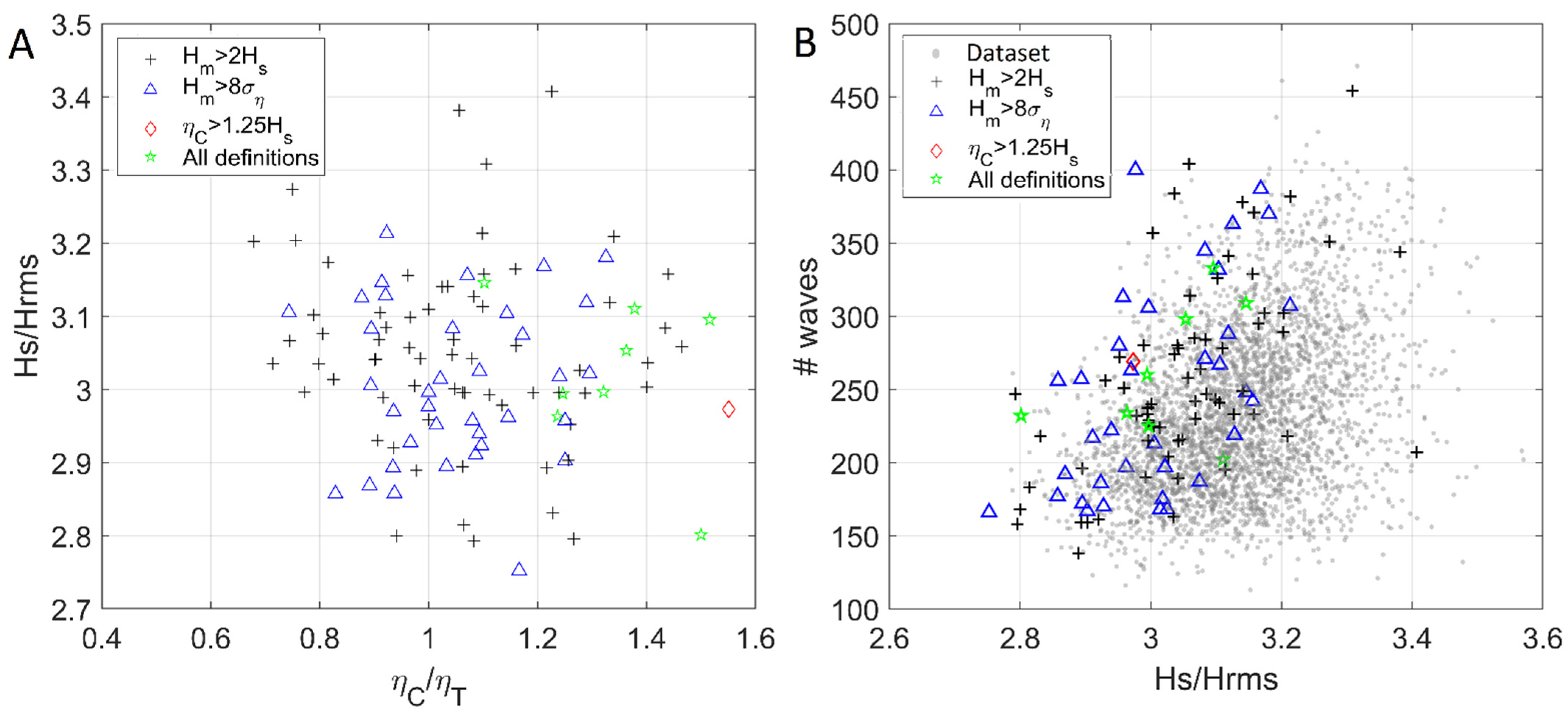
As discussed previously, large ensembles of waves are essential for the identification of rogue waves. It is intended for mainly finding deviations from the almost linear behavior of the waves found in the distribution tail, specifically interesting for our work of those crossing the adopted rogue wave thresholds. Crest-trough symmetry of the analyzed waves is examined in Figure 3; on the left H_s to H_rms ratio is plotted against waves crest to trough ratio of waves that passed the rogue wave threshold, both relating to the same dataset. Only a small number of waves present significant asymmetry, while the most are within the 0.6–1.4 range of the crest to trough ratio. On the right, the ensemble size (number of waves) of each data set is plotted against the H_s/H_rms ratio. The 20 min long ensemble sizes are of 100 to 500 waves, indicating a relatively low statistics population. Additionally, a large scatter of the H_s/H_rms is observed, all in the range between 2.7 and 3.5, indicating transient sea state conditions with amplified nonlinear interactions.

An attempt to increase ensemble size was made by identifying neighboring datasets with similar enough statistical parameters that will justify aggregation into larger ensembles. Figure 4 allows a qualitative inspection of T_m, H_m, H_rms, and H_s (the mean time period, the mean wave height, the root mean square of the waves’ height, and the significant wave height, respectively) variations during the analyzed periods. All parameters are normalized to their respective maximum of each event. The examined parameters show a highly transient behavior for all the events and a persistent lag in the mean time period variations relative to the wave height parameters. These are expected for short-lived stormy events which characterize the weather regime in that area of the Eastern Mediterranean (Figure 1). Based on these findings no ensemble aggregation could be made, and each dataset taken at the hour top was analyzed individually as detailed above.

4. Results

It was concluded from past works and observations that rogue waves are more likely to occur when the sea is high and wave–wave interactions are most dominant [28], under the assumption that wave-wave interactions are one of the main mechanisms responsible for rogue wave occurrences. All high sea event periods are on the order of few days, starting and ending when the sea is considered low as shown in Figure 5.

Table 1. All selected high sea events and their main parameters.

Event Dates	Max. Hs (m)	Max. H (m)	Max. Wind Magnitude (m/s)	Max. Wind Gusts (m/s)	Mean Wind Direction (Deg)	Total Number of Rogue Waves Detected by Threshold H ≥ 2Hs	Total Number of Rogue Waves Detected by Threshold H ≥ 8ση	Total Number of Rogue Waves Detected by Threshold ηc ≥ 1.25Hs
6–10 January 2017	4.31	7.85	15.7	20.3	230	-	2	-
25 January–2 February 2017	6.10	10.01	18.2	23.6	280	3	1	-
15–18 February 2017	2.36	4.00	13.4	16	300	6	-	1
16–22 March 2017	2.38	4.12	13.4	16.3	350	-	1	1
22–28 April 2017	3.32	6.86	10.7	13.2	0	5	3	-
18–27 May 2017	2.51	4.45	9.4	11.7	280	3	3	-
4–12 July 2017	1.84	3.19	7	8.1	300	2	2	2
5–9 September 2017	1.89	3.84	8	9.4	350	2	2	-
21–26 September 2017	1.88	3.13	6	7.3	330	3	2	-
1–20 October 2017	1.87	3.7	8.9	10.4	350	6	6	1
25–31 October 2017	2.00	3.56	10.3	12.5	0	3	-	-
19–26 November 2017	3.89	7.18	10.8	14.9	230	-	-	-
4–9 December 2017	4.03	7.76	12.8	17.8	290	4	2	1
22–28 December 2017	3.71	6.88	13.5	17.3	270	9	-	-
1–8 January 2018	5.04	8.35	17.7	22.3	235	2	-	1
16–29 January 2018	6.62	10.99	15.9	22.1	230	4	3	-
10–22 February 2018	3.03	4.77	15.4	19.4	265	6	2	1
28–31 March 2018	3.36	5.63	14.6	18.9	0	-	1	-
2–8 April 2018	2.02	3.53	10	11.9	95	3	1	-
4–18 May 2018	1.82	3.37	9.7	11.8	10	4	4	1
	Total count					65	35	9

lists the details of the 20 selected events, their main sea and wind parameters, and the count of rogue waves as detected by each threshold.

In Figure 5 variations of the relevant parameters during the selected 20 high sea events are presented on a timeline. The blue and red dots represent the significant wave height H_s and the maximal wave height H_max, respectively. The black dots represent the ratio between the latter and the former. Rogue waves, as detected by the three thresholds, are also marked.

Next, we examined, in detail, the three representative ensembles in which rogue waves were detected (Figure 6), each selected from a different high sea event. The left pane (A, B, C) presents a short period of the water surface elevation fluctuations around the time the detected rogue wave occurs. Each event time series ranked wave height EDF are plotted in the middle panes, compared with the Naess, Tayfun—Fedele 3rd order, Forristall and Rayleigh models EDFs. In the lower panes, the same EDFs are plotted as ln(-ln(p_i)), rendering the distribution linear on the semi-log plot. Such presentation simplifies the examination of the distribution, while the most extreme waves are found in the tail. The vertical line separates the detected rogue waves by 2 times H_s threshold. On the EDF plots, the Boccotti model is excluded as it showed a very large scatter and error due to the variability of sea conditions in each 20 min long ensemble dataset of this high sea event.

In Figure 6 pane A, a relatively low sea condition is observed, characterized by H_s = 1.11 m, and a small rogue wave of H = 2.55 m was detected on 6 July 2017 at about 11:00 a.m. This wave answers all three rogue wave threshold definitions. In Figure 6 pane B, a higher sea condition is observed, characterized by H_s = 2.56 m, and a rogue wave of H = 5.67 m was detected on 23 April 2017 at about 2:00 p.m. This wave answers both (9) and (10) thresholds. In Figure 6 pane C, on 6 December 2017, at about 20:00 a.m., the event was characterized by H_s = 3.63 m and the highest of all detected rogue waves was of height H = 7.76 m.

For these three representative events, four of the models fitted well the empirical data distribution for H/H_s <1.2. In the range 1.2<H/H_s <1.8, the Rayleigh model provided the best fit of the empirical data. While, in the range of the most extreme events, the Tayfun—Fedele 3rd order model performed the best.

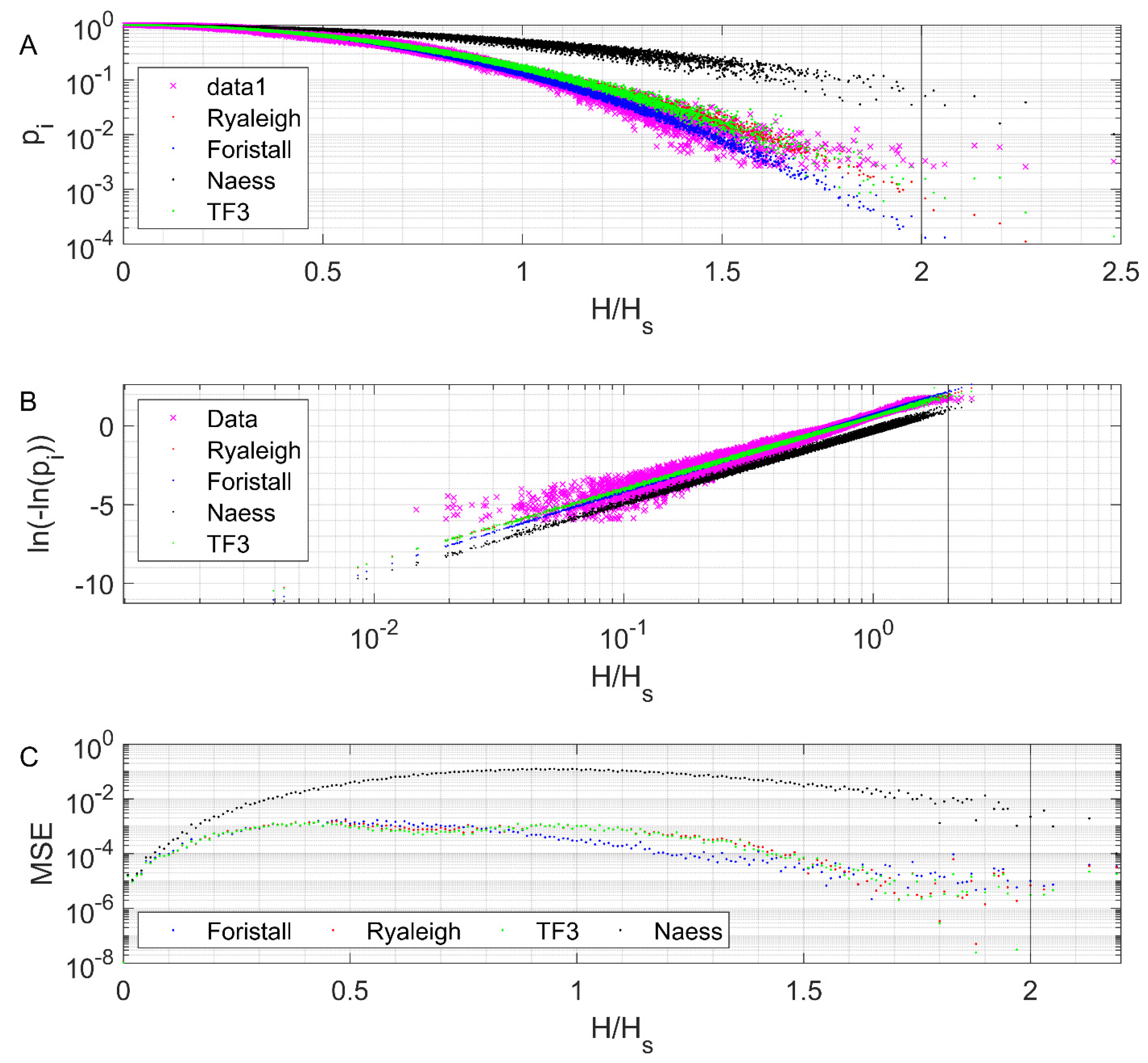
To further examine the performance of each distribution model, we fit all the empirical wave height distribution data during the high sea period with the highest detected rogue wave, the 4–9 December 2017 event. The models were used to fit all the wave height empirical distributions from this storm, and Figure 7 presents the cumulative results. Again, we notice that the Tayfun-Fedele third-order model performance showed the best fit at the tail of wave heights distributions, followed by the Rayleigh and Foristall models. To quantify the selected models’ performance, a mean square error (MSE) of the fits was calculated as:

$$MSE=\frac{1}{n}{\displaystyle \sum {(P_i-P_d)}^2,}$$

(12)

where $P_d$ is the EDF of the empirical data, and all models’ MSE are presented in Figure 7, panel C as average errors over all datasets of this high sea event. MSE values summarizing the models’ performance over the full 18-month period of measurements are presented in Figure 8, also as averages over all available 20 min long ensembles. The Naess model showed errors larger by a few orders of magnitude and therefore was excluded.

In both the December 2017 first event and cumulative MSE of all events in our data, a similar trend was observed. The Tayfun-Fedele third-order and the Rayleigh models demonstrated the smallest MSE in the range of $\mathrm{H}/{\mathrm{H}}_{\mathrm{s}}\le 0.8$, while the Forristall model provided a much better fit for the range of $0.8\le \mathrm{H}/{\mathrm{H}}_{\mathrm{s}}\le 1.5$. Above the ratio of 1.5 and in the distribution tail, the Tayfun-Fedele third-order model performed the best for our data.

Our results suggest that for the examined area of the Eastern Mediterranean during typical winter storms, which result in the most energetic sea state for this area, the Tayfun—Fedele 3rd order is the most suitable parametric model for fitting the empirical data. Showing the best performance for the high waves tail and the lowest waves in the distribution, and comparable performance to that of the Rayleigh model for the middle part of the distribution, the Tayfun—Fedele 3rd order can be recommended for scientific research purposes and engineering modeling of water waves regimes during storms of the coast of Israel.

Finally, we re-examined the crest height-based threshold for the identification of rogue waves. As noted earlier, the threshold ${\mathsf{\eta }}_{\mathrm{c}}\ge 1.25{\mathrm{H}}_{\mathrm{s}}$ assumes that most of a rogue wave water mass is contained above the mean water level, or in other words, most of its energy is carried by the crest. On the right pane of Figure 9, a distribution of all detected rogue wave crest vs. trough heights is plotted. Most of the rogue waves are tightly distributed along the one-to-one line. On the left pane of Figure 9, the ratio ${\mathsf{\eta }}_{\mathrm{c}}/\mathrm{H}$ of all detected rogue waves is presented. The waves are marked in accordance with the threshold to which they correspond, and a 50% ratio signifying equal height crest and trough is marked by a horizontal dashed line. Here, we can note that the majority of the detected rogue waves are distributed within a 40–60% range. Both plots show that among the vast majority of the detected rogue waves there is no preference to crest or trough height.

The crest-to-trough symmetry found in almost all waves identified as rogue by the several commonly used thresholds is not a trivial finding. While comparison with previous reports from the area of the Eastern Mediterranean is currently impossible due to the lack of such reports, which was one of the motivations of this study, our findings are in clear contradiction with the available reports on rogue wave characteristics available from other parts of the world [7,8,9,10,11,12,13,14,15,16,17,18,19,20,21,22]. The rogue waves are commonly reported as having a high crest-to-trough amplitude ratio, indicating strong nonlinearity. Being a statistical rarity, the identification and analysis of rogue waves naturally require large ensembles of waves, hard to achieve in open sea conditions. The here reported results are based on rather small ensembles of 100 to 500 waves (Figure 3). However, the absence of a clear trend or correlation between the ensemble size and the identification of rogue waves, and the lack of observable dependence of the calculated statistical parameters of wave height distribution on ensembles size reassure us that the findings are statistically trustworthy. The disagreement with previous reports cannot be attributed to insufficient ensemble size and different reasoning must be considered.

One such reasoning is the relatively low energetic state of the sea during the here analyzed storms in the East Mediterranean, an area not known for extreme storms. Detected by statistical thresholds, the rogue waves are hence of small height, generally posing no threat to the local maritime transport and rigs. Close examination of Figure 9B shows a slowly increasing trend in rogue wave asymmetry as the wave height increases. As in most cases, a very energetic sea state is chosen in works seeking evidence of rogue wave occurrences; our results call for analyzing existing low sea state data and the deliberate acquisition of new data at similar conditions. Accumulating enough evidence supported by properly quantified statistical parameters will potentially prove further understanding of the trends between sea state and the apparent asymmetry of the rogue waves.

Another reasoning can be found in the discussion regarding the definition of what a rogue wave is. As the name suggests, these waves are also called Freak waves. These are not simply very high waves in the tail end of wave height distribution, but are waves whose characteristics differ significantly from those of the rest of the ensemble. Hence, a somewhat simplistic approach widely adopted for the identification of such unusual waves—a statistical threshold—may not be appropriate to ensure the identified wave is indeed a rogue wave. As mentioned in the Introduction section, very large waves are mostly unaffected by second-order nonlinearities, and hence symmetrical waves at the tail end of wave height distribution will appear symmetric. The empirical evidence analyzed in this study therefore should trigger a reevaluation of the adopted methodology for the identification of rogue waves, to include not only a statistical threshold but also evidence of the wave’s strong asymmetry. However more similar data are needed to initiate the process of reevaluation.

5. Conclusions

Motivated by the lack of sufficient insight and driven by the need for an estimation of possible risks posed by extreme events, the current work provides an overview of the Eastern Mediterranean Sea water wavefield behavior over a period of a year and a half, starting in January 2017. We examined the data provided by a moored buoy, located off the southern coast of Israel. Only the high sea events were analyzed in our search for the best-performing wave height distribution models and to identify and analyze possible rogue wave occurrences. The high sea events were encountered during the winter months, created by the west–southwest storms, as expected in this region.

The performance of five different wave height distribution models in stormy conditions was assessed, comparing their fits to the empirical data. The available data sets were organized in 20 min long ensembles recoded at the top of each hour. The Naess and the Boccotti models showed a large scatter, attributed to the high variability of the sea conditions between the ensembles within each high sea event spanning several days. The Tayfun-Fedele 3rd order model provided the best agreement with the tail of wave heights distribution, while the Rayleigh and the Forristall models showed lesser performances in this range. Following these findings the Tayfun-Fedele 3rd order model is recommended for modeling the local waves field during storms.

This is the first known evidence for the possible occurrence of rogue waves in deep water in this area. The findings indicate that rogue waves may occur during storms in the winter months; however, most of them are of relatively low heights, posing no special concern from the engineering point of view. Even the strongest storm of January 2018, identified by the authors of [18] as a once in 10 years storm, produced waves of below 11 m height and no significant rogue waves. Further work is recommended in the future for a full scope of rogue wave occurrences in the Eastern Mediterranean Sea.

Three commonly accepted statistical thresholds were applied to identify rogue waves. A total of 109 unique rogue waves, (9), were identified. All identified rogue waves were of relatively low height, not exceeding 6 m, while the ratio H_s/H_rms of the ensembles varied between 2.5 and 3.7. The highest wave identified, H = 7.76 m, was a rogue wave detected during a powerful December 2017 storm during which the wave field’s significant height was more than 4 m. A detailed analysis of all identified rogue waves in terms of the crest-to-trough energy distribution revealed that the vast majority of potentially rogue waves exhibited a high level of crest-to-trough symmetry. These findings are in clear disagreement with the widely assumed characteristic of rogue waves as waves with a high crest-to-trough ratio. Moreover, a large number of symmetric, crest-to-trough, waves that crossed the rogue wave threshold at least calls for a reevaluation of the wave crest amplitude-based threshold (11) validity. A slight but steady increase in wave asymmetry at higher sea states stresses the need to conduct a data investigation of low energetic state seas in search of similar evidence. The findings also call for a reevaluation of the commonly accepted rogue wave identification criteria to include not only a simple statistical threshold but also a characterization of wave asymmetry.