Article

Prediction of Water Saturation from Well Log Data by Machine Learning Algorithms: Boosting and Super Learner

by
Fahimeh Hadavimoghaddam
1,
Mehdi Ostadhassan
2,3,*,
Mohammad Ali Sadri
4,
Tatiana Bondarenko
5,
Igor Chebyshev
6 and
Amir Semnani
7
1
Department of Oil Field Development and Operation, Gubkin National University of Oil and Gas, 119991 Moscow, Russia
2
Key Laboratory of Continental Shale Hydrocarbon Accumulation and Efficient Development, Ministry of Education, Northeast Petroleum University, Daqing 163318, China
3
Department of Petroleum Engineering, Amirkabir University of Technology, Tehran 1591634311, Iran
4
Skolkovo Institute of Science and Technology (Skoltech), 121205 Moscow, Russia
5
PetroGuide LLC, 143005 Moscow, Russia
6
Gazpromneft Science & Technology Centre, 190000 Saint-Petersburg, Russia
7
School of Geoscience and Technology, Southwest Petroleum University, Chengdu 610500, China
*
Author to whom correspondence should be addressed.
J. Mar. Sci. Eng. 2021, 9(6), 666; https://doi.org/10.3390/jmse9060666
Submission received: 26 May 2021 / Revised: 9 June 2021 / Accepted: 11 June 2021 / Published: 16 June 2021

Abstract

:
Intelligent predictive methods have the power to reliably estimate water saturation (Sw) compared to conventional experimental methods commonly performed by petrphysicists. However, due to nonlinearity and uncertainty in the data set, the prediction might not be accurate. There exist new machine learning (ML) algorithms such as gradient boosting techniques that have shown significant success in other disciplines yet have not been examined for Sw prediction or other reservoir or rock properties in the petroleum industry. To bridge the literature gap, in this study, for the first time, a total of five ML code programs that belong to the family of Super Learner along with boosting algorithms: XGBoost, LightGBM, CatBoost, AdaBoost, are developed to predict water saturation without relying on the resistivity log data. This is important since conventional methods of water saturation prediction that rely on resistivity log can become problematic in particular formations such as shale or tight carbonates. Thus, to do so, two datasets were constructed by collecting several types of well logs (Gamma, density, neutron, sonic, PEF, and without PEF) to evaluate the robustness and accuracy of the models by comparing the results with laboratory-measured data. It was found that Super Learner and XGBoost produced the highest accurate output (R2: 0.999 and 0.993, respectively), and with considerable distance, Catboost and LightGBM were ranked third and fourth, respectively. Ultimately, both XGBoost and Super Learner produced negligible errors but the latest is considered as the best amongst all.

1. Introduction

Fluid saturation, in particular, water saturation, is a critical parameter for formation evaluation, reserve estimation, and future field planning. The estimated values of water saturation are fed into both reservoir static and dynamic models that are used to estimate original oil/gas in place (OOIP, OGIP) and consequently form the basis for future production forecasts and the determination of the economic viability of the discovered reservoir. Owing to its great significance, water saturation determination has always been an active area of research in petrophysics, and because of that, a variety of methods have been developed through the past decades and are still ongoing. We categorized all these methods into two main categories: (1) direct methods and (2) indirect methods.
Direct water saturation methods are mainly designed and implemented to produce water saturation data. In this regard, (a) laboratory analysis of rock samples and (b) empirical estimation using resistivity log data are the most typical forms. Laboratory-based methods such as Retort method and Dean–Stark and Soxhlet extraction are assumed to be accurate, however, these methods consider the rock sample has representative fluid saturation, which practically is not possible except for very expensive uncommon sampling methods such as sponge core barrel or pressure core barrel [1,2]. In addition, they are exhaustive, time-consuming, and provide discrete data points. For example, the Retort method is a technique of heating crushed core samples up to 650 °C and measuring water and oil volumes driven off. Moreover, Dean–Stark extraction is a technique for measurement of water and oil saturation by distillation extraction when the water in the core is vaporized by boiling solvent, then condensed and collected in a calibrated trap [1]. It can be seen that such methods are destructive, and considering the importance of the samples, they cannot be used in other experiments. Other laboratory approaches such as using rock centrifuge, displacing fluid, and mercury-air capillary pressure curve for a water-air system are expensive, time-consuming, and non-destructive.
Despite the accuracy, laboratory measurements are usually not available for all wells, while log data are commonly acquired in the majority of the wells; furthermore, continuous information across the well is gathered. Determination of fluids saturation is one of the main objectives of well logging, while resistivity is a key to water saturation. In order to utilize resistivity log data for water saturation determination, empirical relations are applied. The most universally practical way is the equation developed by Archie (Archie, 1942) [3,4,5,6], which employs log-driven resistivity and porosity values to compute water saturation. However, this equation was later modified to include tortuosity factor to account for the pore throats in the reservoir, which was shown to be a function of porosity to determine the resistivity factor, given by Equation (1), [1,2,3,4,5]:
S w n = a R w φ m × R t
where a is the tortuosity factor, m cementation factor, n saturation exponent, φ m matrix porosity, R w resistivity and R t is observed bulk resistivity.
What is more, the data represents only the initial state and cannot be used for saturation forecasts. It means that numerical model prediction might be a promising tool for optimization of expenses and filling the gaps in well log data. The exact computation of water saturation using Archie’s formula is based on determination of accurate values of Archie’s parameters a, m, and n. These parameters are ideally assessed from laboratory data. However, these parameters are usually taken as constant values for clean, clastic quartz reservoirs [1], which is not the case that can be found commonly in practice.
Well logging, although very common, could be expensive, thus we may skip running specific tools in a well. There exist cases when a resistivity log is not available due to the tool size limitation. Apart from that, the data obtained from the resistivity log might be unreliable in view of unfavorable geology. In recent years, due to its huge potential, application of machine learning (ML) in geosciences has generated considerable research interest. ML techniques can help to improve petrophysical properties prediction, log interpretation, to optimize core analysis planning and logging service, and to reduce the cost of laboratory measurements. As a result, there has been extensive research regarding the application of artificial intelligence (AI) techniques in well log interpretation [7], shear sonic log prediction [8], and prediction of various reservoir properties such as porosity, permeability, water saturation, lithofacies, and wellbore stability [9,10,11,12,13,14,15].
Numerous studies have shown an accurate prediction of petrophysical parameters from well log data in uncored wells. For example, total organic carbon (TOC) prediction in an unconventional well and permeability estimation in a conventional well were conducted by utilizing support-vector regression (SVR) [16]. Different combinations of gamma ray, formation resistivity, neutron porosity, and bulk density logs underwent training to predict core measurements. Results revealed SVR method accuracy and reliability in TOC and permeability estimation from well-log data. Another ML technique, artificial neural network (ANN), was successfully utilized for permeability prediction from log data in uncored wells [17] and water saturation prediction from wireline logs in sandstone formations [18,19].
Some models revealed a capability in fluids saturation forecasts, cutting expenses on well logging. For example, an unsupervised class-based ML algorithm was utilized to classify the input petrophysical data, such as gamma ray (GR), total porosity (PHIT), effective porosity (PHIE), formation sigma (SIGM), and open hole oil saturation [20]. In this study, seven classes were selected following time series modeling with multiple time-lapse runs on each of the seven selected classes. Next, analyses were conducted using Facebook’s open-source forecasting tool Prophet. Results showed a good validation of oil saturation measurements during a natural depletion period [20].
Some studies proved that there is no need to calculate complex coefficients from Archie’s equation, presenting a good estimation of the water saturation. Authors of the study [21] demonstrated a new approach based on radial basis function neural (RBFNN) for equations of water saturation from four conventional logs, including sonic (DT), deep resistivity (LLD), density (RHOB), and neutron porosity (NPHI) in a carbonate reservoir. It was concluded that the performance of the proposed model is considerably superior to the empirical models, which was also repeated in a similar study [21]. In addition, it was showed by L. Aliouane et al. [22] that the RBF neural network architecture is able to predict formation permeability, porosity, and water saturation using laboratory measurements of the cores and well-log data.
In order to predict water saturation, various machine learning algorithms are utilized. For example, clustering algorithms were proposed and tested on resistivity well-logs in work of [23], namely: fuzzy C-means clustering, Gustafson–Kessel algorithm, and Gath–Geva clustering. The authors chose unsupervised methods because they do not require real labeled data. Study [24] presented an application of the local linear neuro-fuzzy (LLNF) model in estimating reservoir water saturation from well logs. This was followed by [25] aiming to evaluate fluid saturation in oil sands by means of ensemble tree-based algorithms. Later on [26], support vector machine, decision tree forest, and tree boost methods were employed to predict water saturation of Mesaverde Tight Gas Sandstones located in Uinta Basin. In paper [27], the multilayer perception (MLP-) and kernel function-based least-squares support vector machine (LS-SVM) techniques were utilized to develop predictive models for water saturation. Furthermore, an intelligent structure named robust committee machine (RCM) for water saturation prediction was introduced [28].
Various well log data and petrophysical properties measured in the lab are used as input parameters in different algorithms to predict water saturation in sandstone and carbonate reservoirs. For example, a water saturation model was constructed based on the lithofacies identified in different wells [29], or ANN was developed to predict a water saturation, while porosity, permeability, and height above free water level were used as the input data [30].
Among the machine learning methods used in practice, gradient tree boosting [31] is a technique that stands out in many applications. This method is also known as gradient boosting machine (GBM), or gradient boosted regression tree (GBRT). In the last two decades, boosting algorithms have been the most widely used ones in data science to achieve state-of-the-art results [32,33,34]. Boosting is a meta-algorithm based on an idea of gradually aggregating numbers of simple algorithms, called weak learners, to obtain a final strong learner. More specifically, each weak learner is optimized to minimize the error on the training data using the sum of the previous weak learners’ predictions as an additional input [35,36]. This is conducted by dividing the training data and using each part to train different models or one model with a different setting and then using a majority vote, the results are combined together. The Adaboost was the first successful method of boosting discovered [37,38] for binary classification. Based on the work of Friedman [31], who introduced gradient boosting of decision trees, several implementations have been recently developed. Three effective methods of gradient boosting based on decision trees have been proposed, namely: XGBoost [39], CatBoost [40], and LightGBM [41].
Following what was said above, AdaBoost can be useful for comparatively small datasets, while scalable algorithms are required for much larger datasets. To resolve this requirement, XGBoost, LightGBM, and CatBoost are intended to be employed. XGBoost is a parallel tree boosting system, which is designed to be more flexible and portable and efficient. XGBoost applies the loss feature to a regularization term that helps construct more generalizable versions. In return, XGBoost is the most recently used algorithm from a design viewpoint to model proxy reservoir simulations. Many researchers recently declared the successful implementation of boosting algorithms applications in petrophysics and reservoir characterization as the proof of reliability to be applied for water saturation prediction [42,43,44,45,46]. Another powerful and flexible implementation of tree-based gradient boosting is LightGBM, such as XGBoost. To maximize concurrent learning, it leverages network connectivity algorithms. To speed up the training process and decrease memory usage, it utilizes a histogram-based algorithm. Additionally, instead of level-wise, LightGBM grows trees leaf-wise. In ensemble learning, the tree growth technique is usually level-wise, which can be an inefficient method. Although XGBoost and LightGBM provide several benefits, CatBoost may provide a more effective approach while remaining scalable when a large number of categorical features are present in the dataset [41].
The new approaches were successfully employed in business, academia, and competitive machine learning [47]. While built on structurally similar ideas, these libraries slightly differ on how decision trees are grown or how categorical variables data are handled, and only investigation can validate which performs best. Ensemble modeling is a robust method to enhance the model’s performance. Super Learner [48,49] is known as stacking ensembles. Van der Laan et al. [48] was the first who proposed this algorithm in biostatistics, while Polley and van der Laan [49] developed the detailed algorithm.
In the petroleum industry, there could be a significant prediction error in a single machine learning model while another could perform well. Authors believe Super Learners can further enhance predictive ability by stacking prediction results from algorithms that learn from the base algorithm. Therefore, although huge research has been carried out in recent years, the accuracy of prediction should be improved by testing more machine learning techniques and their combinations, e.g., in petrophysics. Hence, the purpose of this study is to describe and examine boosting methods for water saturation prediction compared with the Super Learner that has never been examined before, to the best of our knowledge, due to its newness. Moreover, we aimed to remove the dependency of such predictions on resistivity logs, which are necessary for water saturation determination. Finding an accurate prediction model will reduce the cost of core-based measurements and well-logging services. Ultimately, it will increase the accuracy of well log interpretation, where a certain type of data could be missing.

2. Methodology

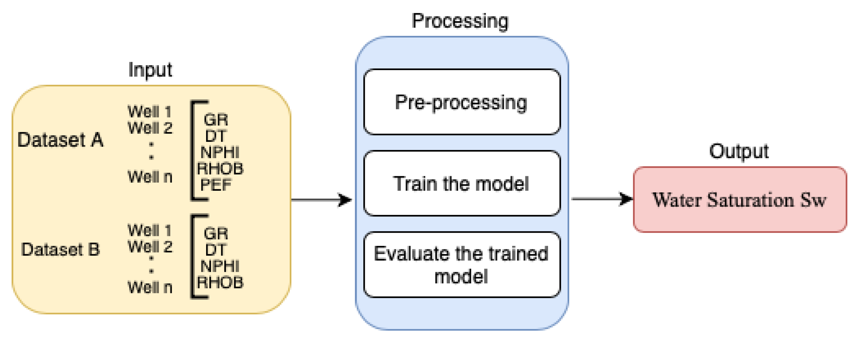
2.1. Dataset Preparation

Well log data (Gamma, density, neutron, sonic, PEF) from 11 wells drilled in a sandstone reservoir in the Russian Federation were used for this study and considered as a feature (including the entire log dataset) to develop the model, while 7 wells out of 11, were used for training the model and the rest for final validation.
On the input dataset, we used a 4-fold cross-validation scheme. To begin, each dataset was divided equally into 4 folds at random, and the distribution of each fold was tested to ensure there were no substantial variations in the distribution of the entire dataset. One-fold of samples was used as test or evaluation data for each iteration, while the remaining 3 folds of samples were used as training to match the model. On validation data, the fitted model was then used to predict water saturation. The iteration process proceeded until all sample folds were expected. In this case, all samples in the dataset were predicted using the model fitted without being used as training data themselves. This method of cross-validation scheme eliminated the possibility of overfitting to a fixed train dataset while simultaneously ensuring that all datasets were used to their full capacity. For better representation, a schematic of K-fold cross-validation is shown in Figure 1.
Two separate approaches, one by including and the second one by excluding the PEF log, along with their corresponding datasets, were created and labeled, A and B, respectively. This was conducted to examine if tested ML methods can produce results with the least dependency on input data, especially those that might not always be available in petroleum industry more frequently, here PEF (photoelectric factor). To create the datasets, 5 readily available different well logs including: GR, sonic (DT), neutron-porosity (NPHI), formation density (RHOB), and photoelectric factor (PEF) were used for input into the algorithms. Two different approaches, as stated earlier, were carried out, which involved developing different ML techniques using data sets A and B, respectively. While both datasets benefitted from having 7 training wells and 4 blind tests, where the input features for dataset A were GR, DT, NPHI, RHOB, and PEF and for the dataset B, only GR, DT, NPHI, and RHOB. This was conducted based on the fact that first, we would like to examine the hypotheses of removing the dependency of our prediction on the resistivity log although it was available in all wells and was the basis for water saturation estimation, and second, if some lesser common logs, here PEF, can also be ignored too. In Figure 2, the process of constructing the ML models is illustrated.

2.2. Calculating Water Saturation
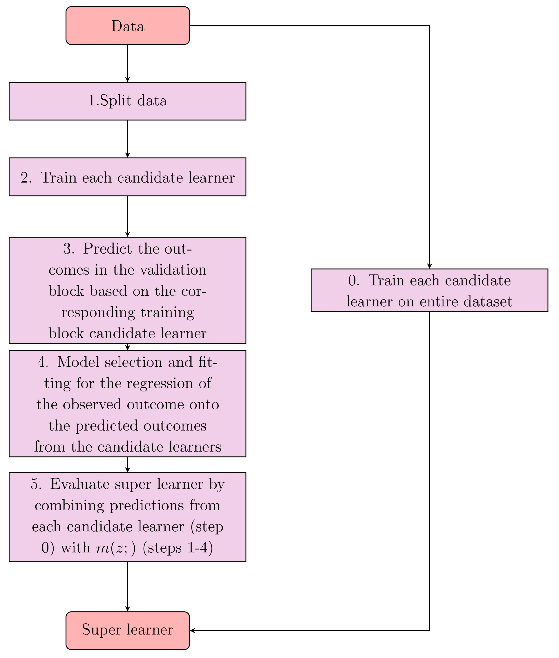
The Archie equation was used to calculate the water saturation through Dean–Stark data that was available for the formation understudy in 2 wells. The Archie estimated value of water saturation that was obtained in the lab was set as the target value, while the resistivity calculated water saturation was also calculated. It was observed in Figure 3 that the interval was clean with low GR readings reflecting a sandstone formation. Hence, the Archie equation should work well without any need to use complex empirical relationships for the estimation of water saturation. Furthermore, water saturation was also measured in 2 of these wells from plugs that were preserved and tested in the lab. As we can see in Figure 3 there was a good match between the experimental value of Sw and predictions by Archie equation, shown on the fourth track. In this track, blue dots represent experimental data and the red curve was calculated water saturation through Archie’s equation with m = 1.49 (cementation factor), n = 1.82 (saturation exponent); a = 1.532 (tortuosity factor) and Rw = 0.35 (formation water resistivity). These parameters for accurate utilization of the Archie equation were based on knowing/measuring them and were found in laboratory studies for the formation understudy. Determination of Rw in the application of Archie’s method is the main problem when there are not enough production tests and sample water, which fortunately was not the case here. The other disadvantage of Archie’s method was that when the rock matrix type is unknown, it can impose significant error into the results. This issue can be addressed by having the PEF log, which provides us with direct knowledge about the lithology (dominant lithology) of the formation. Additionally, since there is an inherent uncertainty in estimations of m, a, and n values, extensive experimental analyses are required. Ultimately, in the case when these parameters specific to the formation are not available, assumptions can be made, which will introduce errors to the final water saturation calculated results. Please note, in order to avoid a lengthy manuscript and deviate from the main idea in the study, we decided not to include steps that were taken to estimate Sw by the conventional Archie’s equation since this is a routine process that can easily be found in all petrophysics and reservoir engineering books [50].

2.3. Methods

Boosting is extremely an effective machine learning technique in its dependency on input data, using them and generating final outputs [42]. In this paper, we developed code programs based on 4 boosting methods: XGboost, LightGBM, Catboost, and Adaboost, in addition to the Super Learner, a total of 5 different algorithms to compare the accuracy of water saturation predictions across the board. All calculations were carried out using Python programming language where respective Python packages and their versions are listed in Table 1 (developed python code programs can be provided upon request). The Super Learner is distinct from other machine learning algorithms since it is simply a base learners combination algorithm. In this context, any other machine learning algorithm such as XGboost, LightGBM, Adaboost, and Catboost can be a base learner of a Super Learner algorithm. In our study, 2 machine learning algorithms, including: XGboost and LightGBM, were utilized as input parameters in the Super Learner ensemble.

2.3.1. Models

Boosting, like bagging, is a common method for regression or grouping that can be extended to a large number of base learners. In boosting, base learners (in our case, trees) are given training iteratively to increase focus on findings that the current aggregation of base learners fails to model well. Similar boosting algorithms calculate misclassification differently and choose various settings for the next iteration. The primary goal of boosting is to minimize bias. Because of the increased emphasis on misclassified cases, the bias part of the mistake was minimized. AdaBoost is the most widely used boosting process [51,52], which trains models in such a way that misclassified examples were found at the end of each iteration, and their importance was increased in a new training set. This set is then fed directly into the next iteration’s beginning.
The gradient Boosting method, unlike AdaBoost, fit the base-learner to the negative gradient of the loss function measured in the previous iteration rather than re-weighted cases. Although AdaBoost and GBMs are effective for small datasets, scalable algorithms are needed for far larger datasets. This condition is addressed by XGBoost, LightGBM, and CatBoost.
The main steps of Adaboost methods is represented below:
  • Defining Weights: w j = 1 n ,   j = 1 , 2 , , n ;
  • For each i, define the training data to a weak learner Wl i x using weights and determine the weighted error
  • Err i = j = 1 n w i I t j wl i x j = 1 n w j , I x = { 0   if   x = false   1   if   x = true
  • For each i, estimate weights for predictors as: β i = log 1 Err i Err i
  • Updated data wights for each i to N (N is the number of learner);
  • Adjust weak learner for data test (x) as output.
XGBoost is a parallel tree boosting framework that is available in large, distributed environments such as Hadoop and is designed to be highly powerful, scalable, and portable. Thanks to improvements over GBMs, such as the introduction of split finding algorithms for sparse data with nodes’ default directions and fast enumeration of all feasible splits to maximize the splitting threshold, it can solve problems with billions of instances. XGBoost also has a regularization concept in the loss feature, which aids in the development of more generalizable models. In terms of architecture, XGBoost has recently been used to simulate steel fatigue resistance and surrogate reservoir simulation [53]. To model the performance y for a given dataset, an ensemble of n tresses should be trained according to the following expression, depicted in Figure 4:
y ^ i = k = 1 N f k X i ,   f k f .
With f X = ω q x ,   q :   m T ,   ω     T , where example x is represented by the decision rule q(x) to the binary leaf index and f declares the space of regression trees; ω the weight of the leaf; fk the kth independent tree; and T is the number of leaves on the tree.
LightGBM, such as XGBoost, is an effective and scalable tree-based gradient boosting implementation. It optimizes parallel learning by using network connectivity algorithms. It uses a histogram-based algorithm to reduce memory usage and speed up the training process. Furthermore, LightGBM grows trees leaf-by-leaf rather than level-by-level. In most cases, the tree growth technique used in ensemble learning is level-wise, which is inefficient [54].
While XGBoost and LightGBM have several advantages, when a dataset contains a large number of categorical attributes, CatBoost could be a more effective and scalable solution. CatBoost employs oblivious decision trees, a form of level-wise expansion. It implements a vectorized representation of the tree in this extension, which can be tested quickly. CatBoost also improves algorithmic performance by using ordered boosting, a permutation-driven alternative to the standard boosting algorithm, and a variety of target statistics for categorical function processing.
Polley and van der Laan [49] created the Super Learner algorithm. A diagram of the Super Learner algorithm is shown in Figure 5 below to make the algorithm simpler. Since it is a hybrid algorithm with base learners, Super Learner is unlike any other machine learning algorithm. Any machine learning algorithm, such as XGBoost or LightGBM, may be used as the base learners of a Super Learner algorithm. After that, the base learners are selected and configured separately using train data.

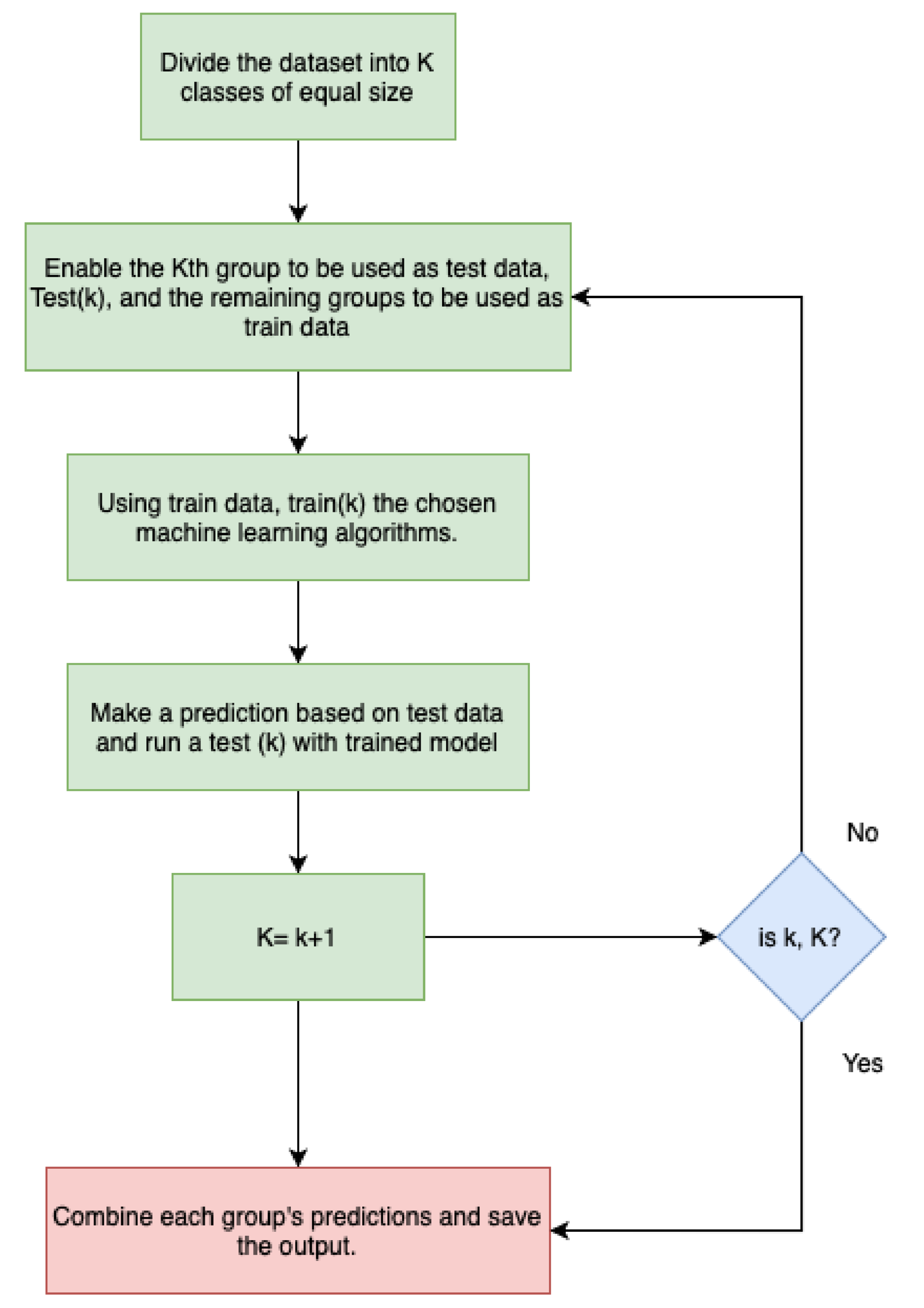
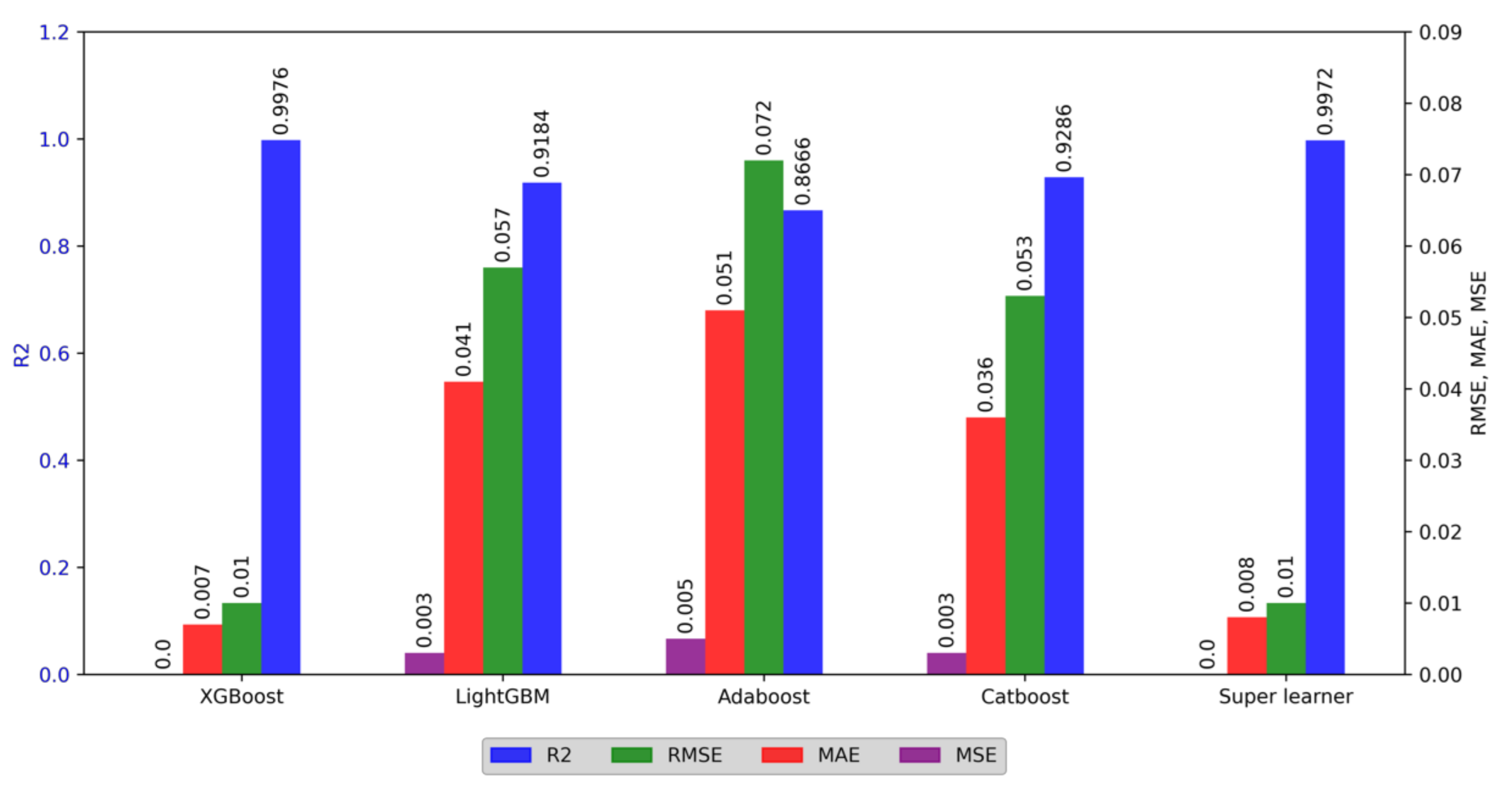
2.3.2. Model Evaluation

In Table 2, min-samples-split, n-estimators, max-depth, min-samples-leaf, learning rate, colsample-bytree, subsample, num-leaves, depth, and iterations are the minimum number of samples required to split an internal node, number of trees, maximum tree depth, minimum number of samples needed at a leaf node, learning rate, column subsample ratio when building a tree, fraction of observation ratio when building a tree.
The prediction performances of AI models highly depend on the quality of the input data. Before feeding any data to the AI system, data analysis and pre-processing steps were performed. Data pre-processing step involved statistical ways to remove outliers and unrealistic values that are highly recommended in ML methods and taking advantage of AI techniques [55,56]. To estimate the accuracy of the model, 4-fold cross-validation was performed. In this study, the robustness and accuracy of the models have been evaluated using different popular evaluation metrics: the coefficient of determination (R2), mean squared error (MSE), mean absolute error (MAE), and root mean squared error (RMSE) [56,57,58], each defined by the following equations:
Root mean squared error (RMSE) metric is given by Equation (2):
RMSE = i = 1 N Actual i   Predicted i 2 N
where, N is total number of observations. Mean squared error (MSE) metric is given by Equation (3):
MSE = i = 1 N Actual i   Predicted i 2 N
Mean absolute error (MAE) metric is given by Equation (4):
MAE = i = 1 N Actual i   Predicted i N
Considering these error numbers, the lower the value of RMSE, MSE, and MAE metrics, the better the model would be. Finally, the coefficient of determination (R2) metric is given by Equation (5):
R 2 = 1 Actual i   Predicted i 2 Actual i mean   of   the   observed   data 2
Best possible R2 score is 1.0. A constant model that always predicts the expected value, disregarding the input data, would reach a score of 0.0.

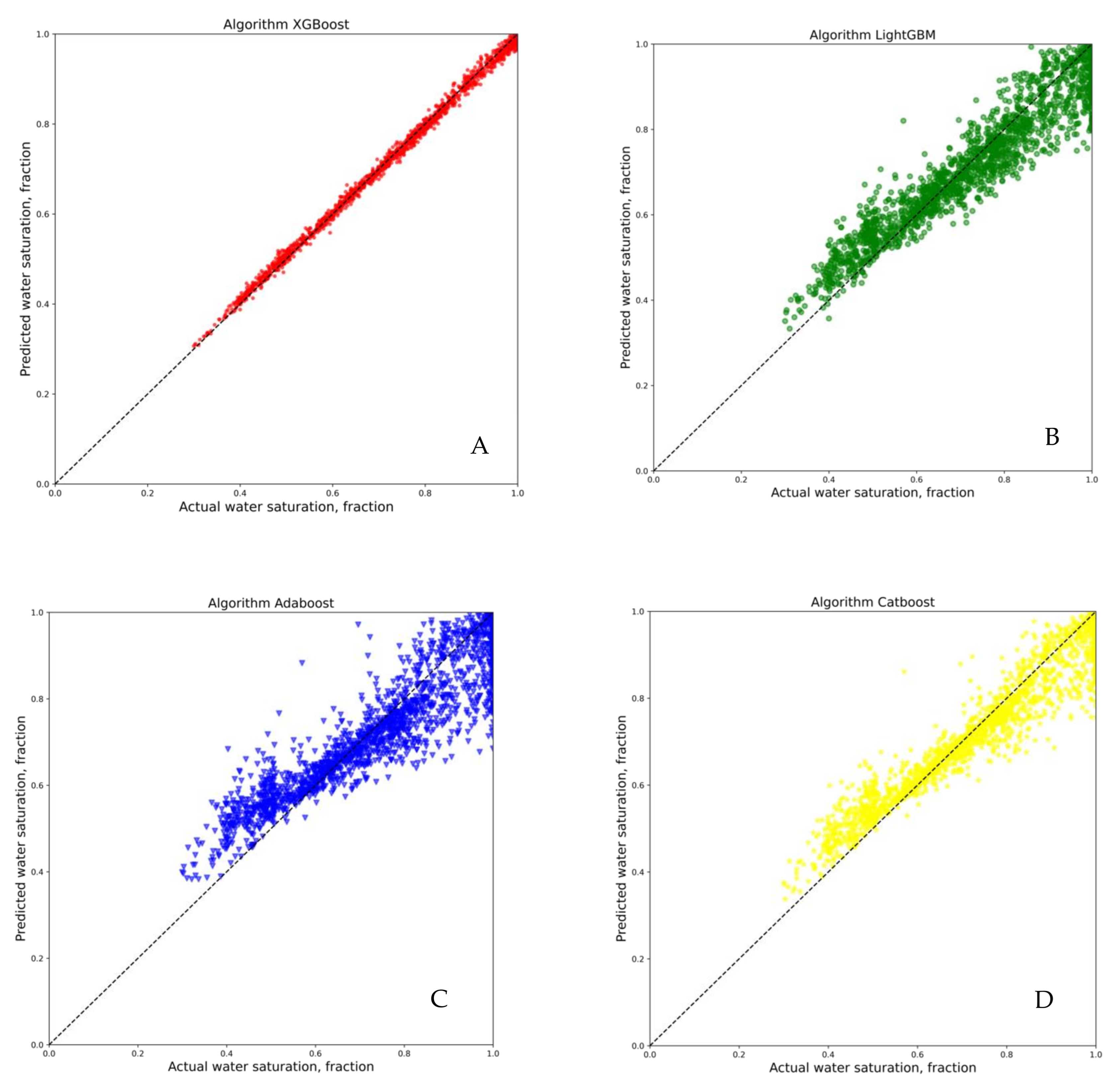
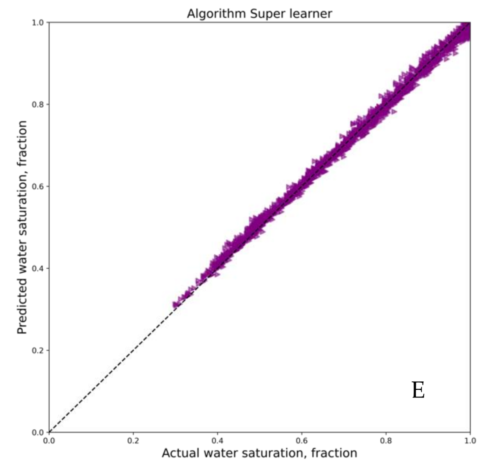
3. Results and Discussion

To evaluate the performance of each ML method, the metric evaluation was applied. Table 3 summarizes the evaluation metrics summary. As can be seen from these values, the Super Learner algorithm prediction was the most accurate one, while Adaboost showed the least favorable results. Figure 6 is the cross-plot of actual water saturation measurements vs. the predictions for various algorithms used here, while Figure 7 provides the bar plots of evaluation metrics for better visualization. We can see that Super Learner and XGBoost have the lowest error values, while Adaboost has the highest error. Based on the obtained results, it is apparent that there is no need to calculate complex coefficients such as cementation factor, tortuosity factor, saturation exponent that are required when using Archie’s equation for estimating water saturation.
Collectively, comparing the data, it can be seen that XGboost and Super Learner could be promising tools in water saturation prediction from the well log data. The performances of the ML techniques for the prediction of water saturation (dataset A) are summarized in Table 3, and it can be noticed that most leading techniques in each category can be used with confidence. It should be noted that in the following figures, Archie calculated water saturation based on parameters that were measured in the lab and verified when experimental data are plotted vs. AI estimated values.
Based on Figure 6, which is the cross-plot of target values vs. prediction outcomes, it is observed that there is an excellent correlation between these two values by Super Learner method. The metric evaluation of using different machine learning algorithms is also shown in Figure 7. Additionally, Figure 8 explains that Super Learner is the best choice for estimation of water saturation without resistivity logs being used as an input parameter as well as the XGboost with comparable performance. Although the discrepancy between various metric values of the algorithms that were utilized are not significant, Super Learner still performs better than the rest of the algorithms. On the contrary, Adaboost and Catboost exhibited the highest estimated errors. As shown in Figure 6, Figure 7 and Figure 8, based on the results, Super Learner ranked the first in all performance judging criteria and XGboost ranked the second. Again, it should be reminded that the performance is the level of matching results in experimentally obtained water saturation values vs. the predictions. Please note the results containing all test wells through cross plotting predictions vs. measurement of water saturation are depicted in the Appendix A for dataset A for Well 1 to 3.
In dataset B, the PEF log is kept out of being input in predictions. It should be noted that the PEF log is not as common as other well logs used here while it provides us with direct clues about the formation lithology. Knowing formation lithology is vital for estimating porosity based on the rock physics models from neutron and density logs. The performances of the ML techniques for the prediction of water saturation (dataset B) are summarized in Table 4 where the most leading techniques in each category are revealed based on the error values they generated.
In dataset B, as it was mentioned, four well log suites were used as input features for estimation of water saturation. In dataset B, it was decided to leave the PEF log out of the input features. This was decided based on the fact that the PEF log might not be available and is not as commonly acquired in wells as the rest. The results illustrate that if input features from five well log suites are reduced to four well logs, the overall performance of ML techniques will not be affected notably across the board. Hence, water saturation can still be predicted with high accuracy. Based on metric analysis (Figure 9) and cross-validation (Figure 10), Super Learner and XGboost have the lowest error and the highest accuracy among all algorithms. Moreover, Figure 11 represents the results for five algorithms presented as a well log format (continuous estimation of water saturation) for the entire interval. Please note the results containing all test wells through cross plotting predictions vs. measurement of water saturation is depicted in the Appendix B for dataset B for Well 1 to 3.
With a more detailed analysis of these graphs (Figure 9, Figure 10 and Figure 11), we can conclude the reliability and precision of these predicative models collectively. Various statistical parameters, including correlation coefficient and relative errors, are used as a comparison basis to make judgments to see if predictions and experimentally measured values would match. The predictive model for dataset B in the absence of PEF log variable leads to high performance since the PEF log has a lower impact than other variables. Its lowest impact, although its importance was found in the results but also confirmed through sensitivity analysis as well. Consequently, it might be unnecessary to include an additional correlating parameter as an input feature for the prediction of water saturation. According to the statistical analysis of feature importance shown in Figure 12, conducted for the Super Learner approach, the decreasing order of importance of input variables for predicting water saturation would be as follows: gamma ray, sonic log, porosity, and bulk density, and photoelectric factor log while the latest one was found optional.
Iteratively, boosting approaches train a series of weak learners, where the weight of the records is modified according to the regression effects of the previous learners’ loss function. In terms of CPU runtime and precision, we compared three state-of-the-art gradient boosting methods in this study. Using the same hyper-parameter optimization time budget, XGboost is more accurate in predicting water saturation for the studied dataset, and LightGBM appears to be considerably faster than the other gradient boosting strategies (Table 5). Super Learner was designed for this study with two base learners, such as XGBoost and lightgbm. The idea of a Super Learner is appealing, making it possible to train and test a multitude of machine learning models on a single collection of data and thereby allowing the model to optimally integrate any of the individual models to produce better overall predictions. In this article was investigated small aspects of the protentional of combining ML algorithms.
The XGBoost technique also leads to almost the same findings and highly comparable to Super Learner based on the overall error analysis and matching the predictions with true values. In the literature, it is claimed that resistivity (RT) and porosity logs (neutron or density) are essential to determine water saturation using petrophysical models. According to the current study, the minimum log variables were used for the estimation of water saturation, which was not attempted previously. The engineers and/or operators in the oil and gas industry can utilize the developed deterministic approaches using the data from the most contributing and available common well logs as listed here for prediction of water saturation to save the exploration expenses and time in an effective manner.

4. Conclusions

This article demonstrates the idea of the application of machine learning algorithms, such as XGBoost, LightGBM, AdaBoost, CatBoost, and Super Learner, to predict water saturation from well-logging data. The study revealed that XGboost and Super Learner might be promising tools in water saturation prediction from well log data collected by the authors without relying on a resistivity log. These methods can be applied to reduce the cost of core measurements and well-logging services. In all combinations of predictors considered, Super Learner is proved to be useful to combine the merits of base machine learning algorithms and enhance predictive robustness on water saturation.
In addition, it has the potential to increase the accuracy of well logs interpretation in wells, where some data are not available. Two different datasets were used in this study to observe the effect of diverse variables. The additional correlating parameter (PEF log) has not convincingly improved the performances of ML techniques for the prediction. The main advantage of using machine learning and intelligent methods in estimation water saturation is that with knowing examples of previous patterns, they can be easily trained and put to effectively solve unknown or untrained instances of the problem. In addition, there is no need to calculate the complex coefficients such as cementation factor, tortuosity factor, saturation exponent, etc. The results confirm the performance of the proposed ML models in estimation water saturation, particularly never applied super leaner. In addition, in this study, estimated water saturation was achieved without relying on resistivity log, which could be challenging to certain geological structures. The proposed model can be employed in several applications of static reservoir modeling, such as porosity and permeability prediction in the future.

Author Contributions

Conceptualization, F.H. and M.O.; methodology, F.H., M.A.S. and T.B.; software, M.A.S. and I.C.; validation, T.B., F.H. and A.S.; formal analysis, F.H., A.S. and T.B.; investigation, F.H.; resources, I.C. and M.O.; data curation, M.A.S. and F.H.; writing— original draft preparation, F.H. and M.O.; writing—review and editing, M.O.; visualization, F.H.; supervision, M.O.; project administration, M.O.; funding acquisition, M.O. All authors have read and agreed to the published version of the manuscript.

Funding

This research received no external funding.

Data Availability Statement

Data can be provided upon request to corresponding author.

Acknowledgments

Authors would like to sincerely thank Gazporomneft for providing us with the data and allowing us to publish them. Furthermore, we appreciate input by anonymous reviewers and respected editor for constructive comments that significantly improved this manuscript.

Conflicts of Interest

Authors declare no competing interest.

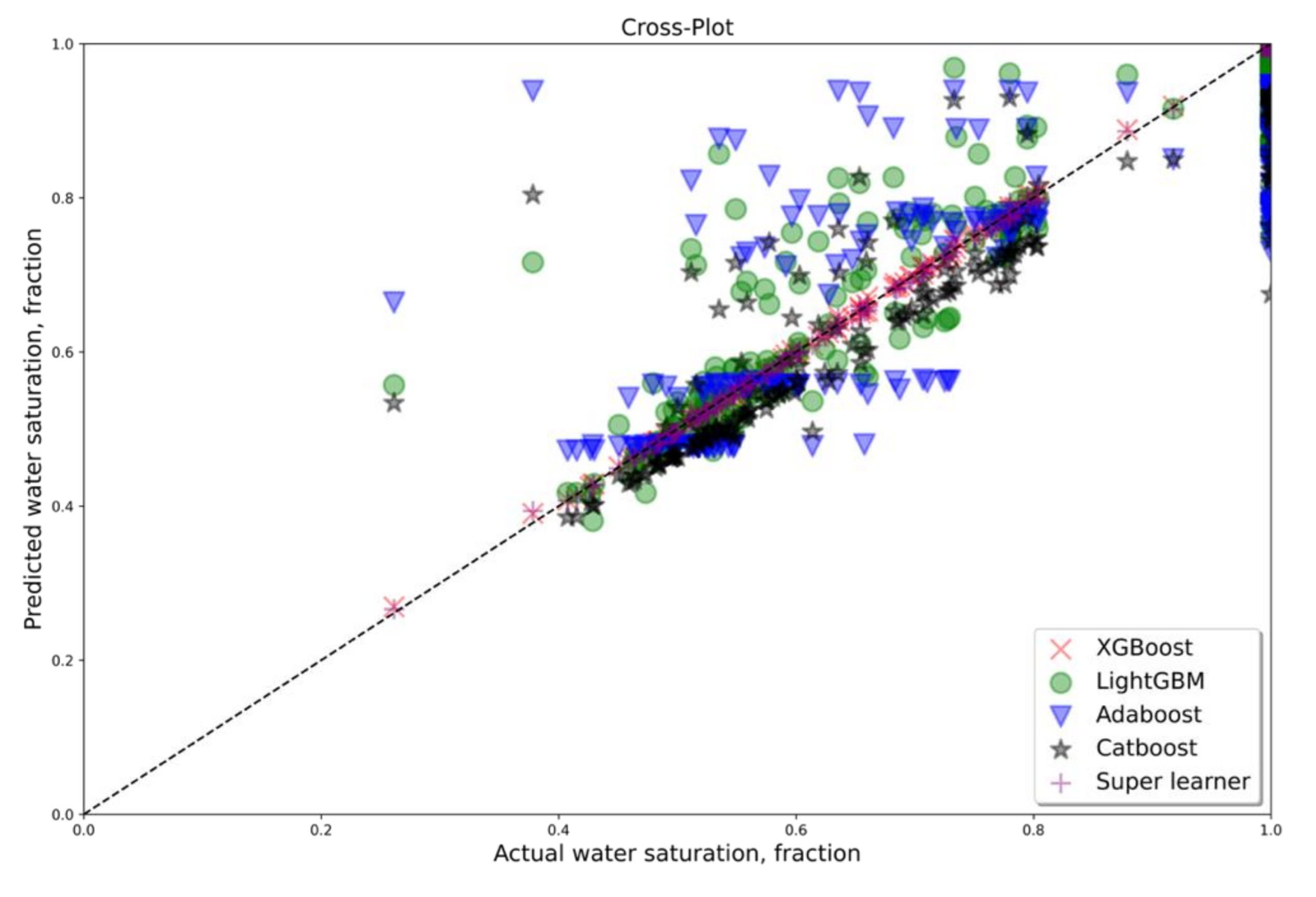
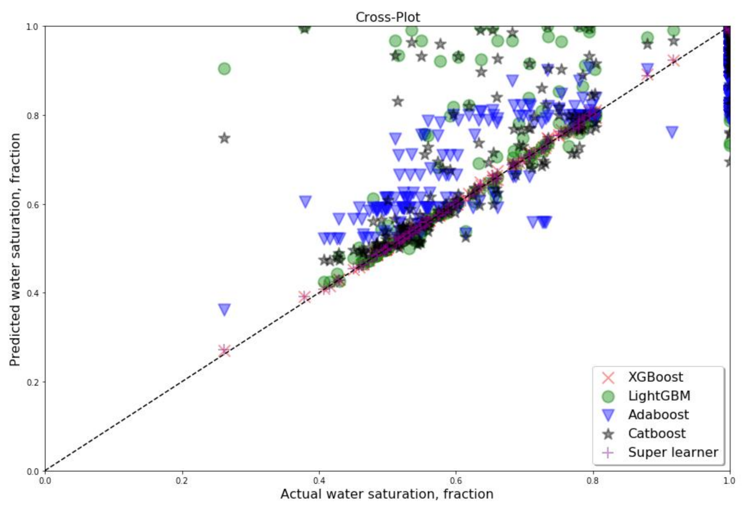
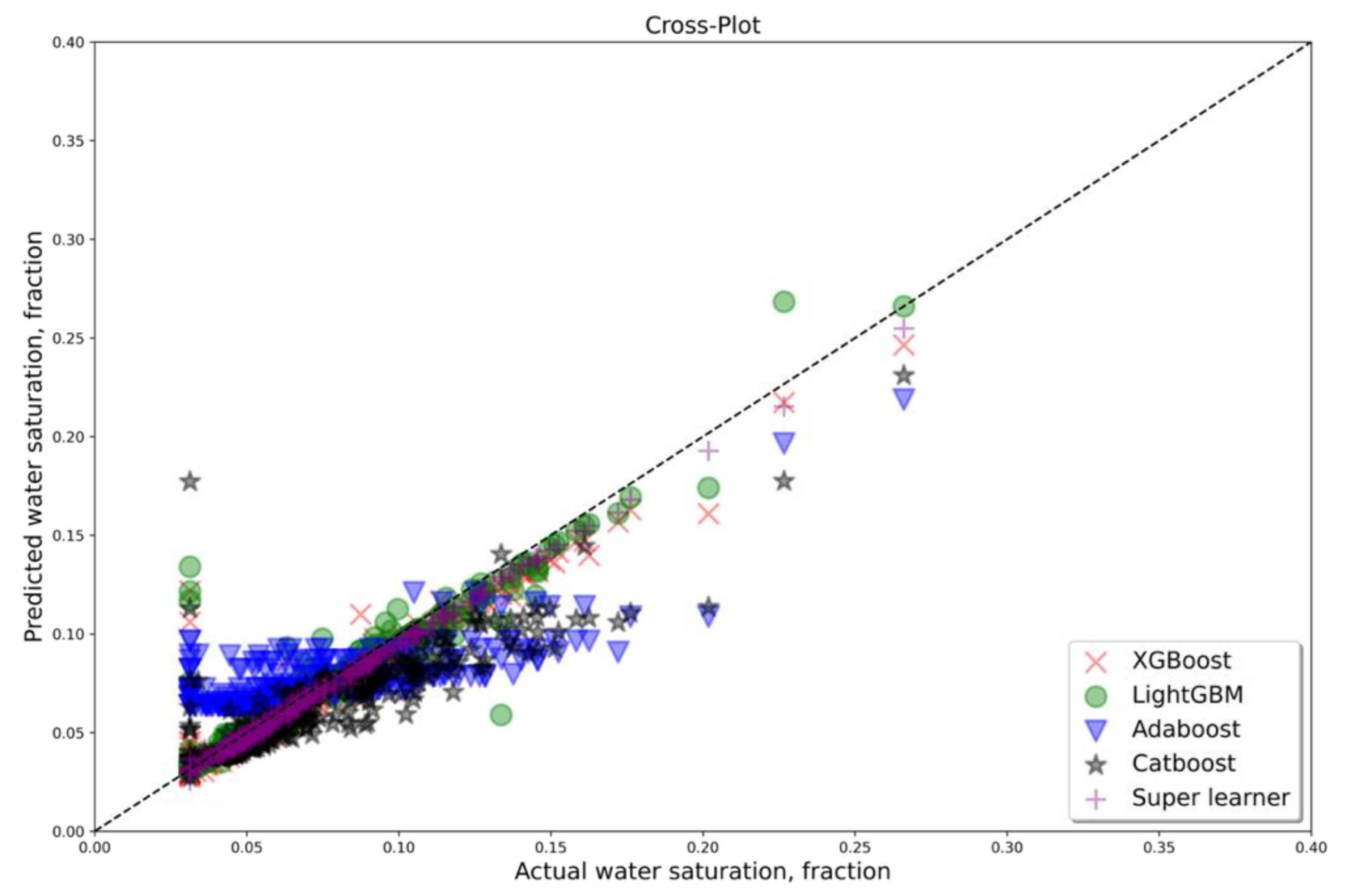
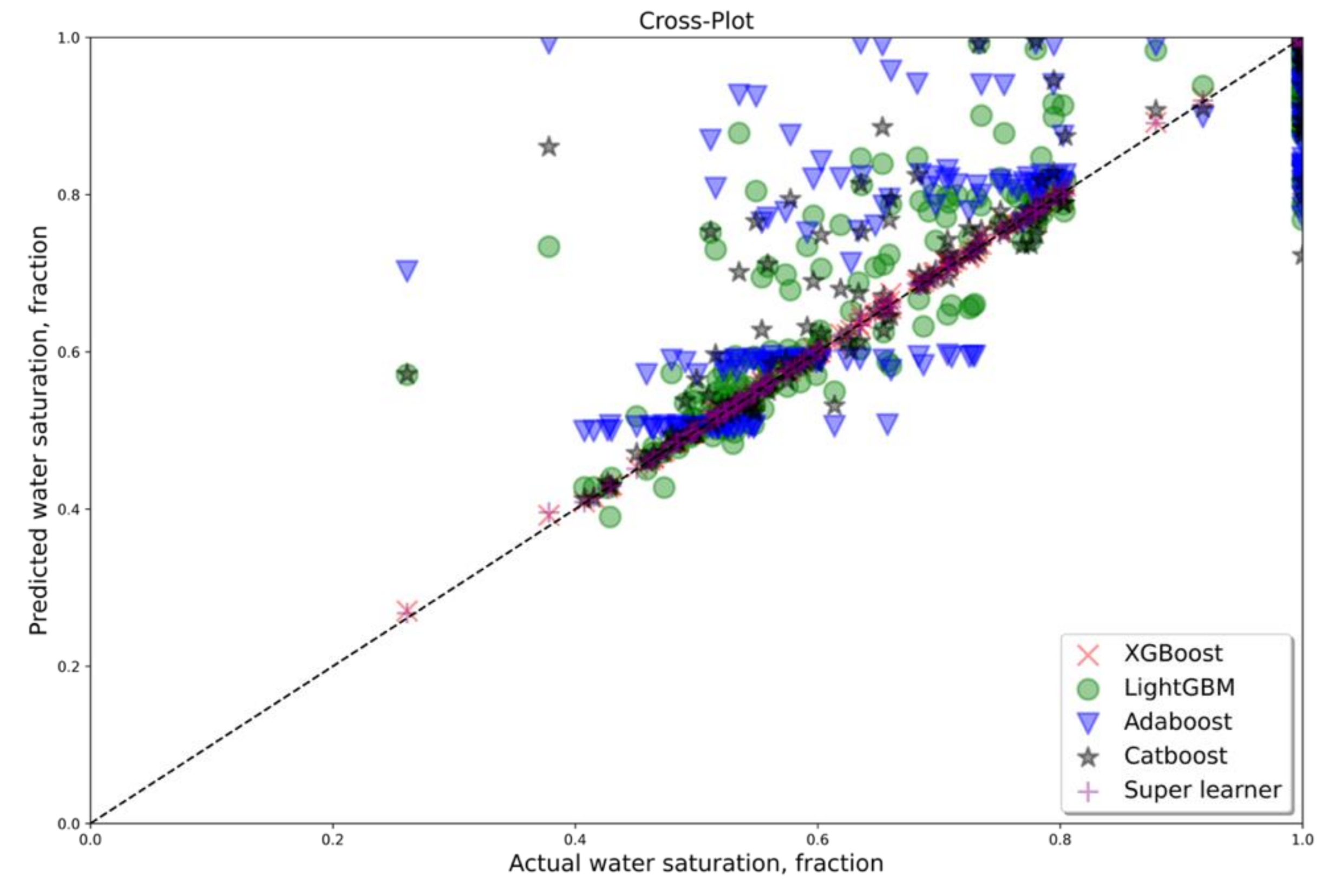
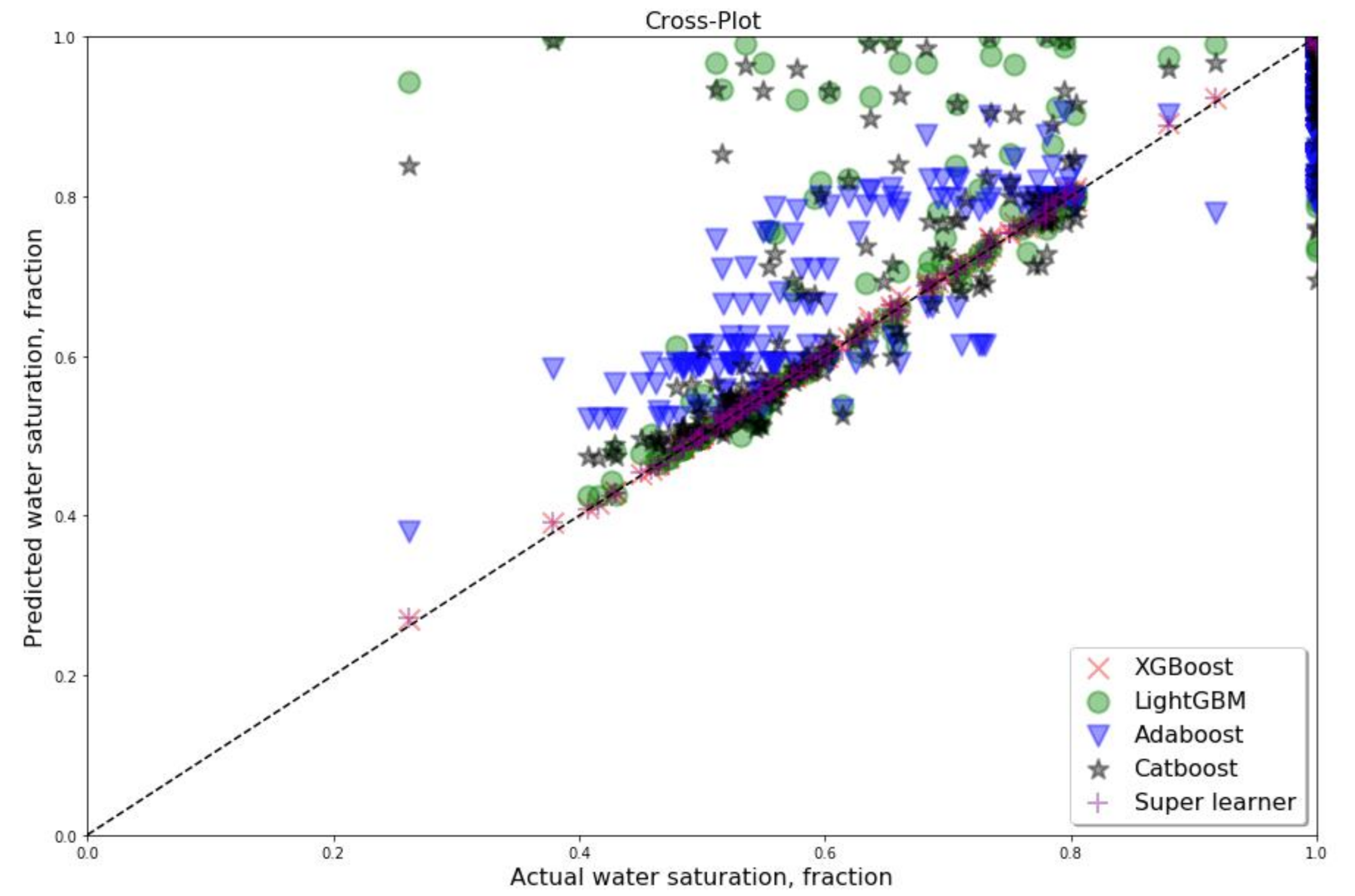
Appendix A. Cross Plots for All Well, Which Were Considered as Testing for Dataset A with Five Features (PEF Included)

Figure A1. Cross plot for water saturation prediction results by different algorithms (Well 1).
Jmse 09 00666 g0a1
Figure A2. Cross plot for water saturation prediction results by different algorithms (Well 2).
Jmse 09 00666 g0a2
Figure A3. Cross plot for water saturation prediction results by different algorithms (Well 3).
Jmse 09 00666 g0a3

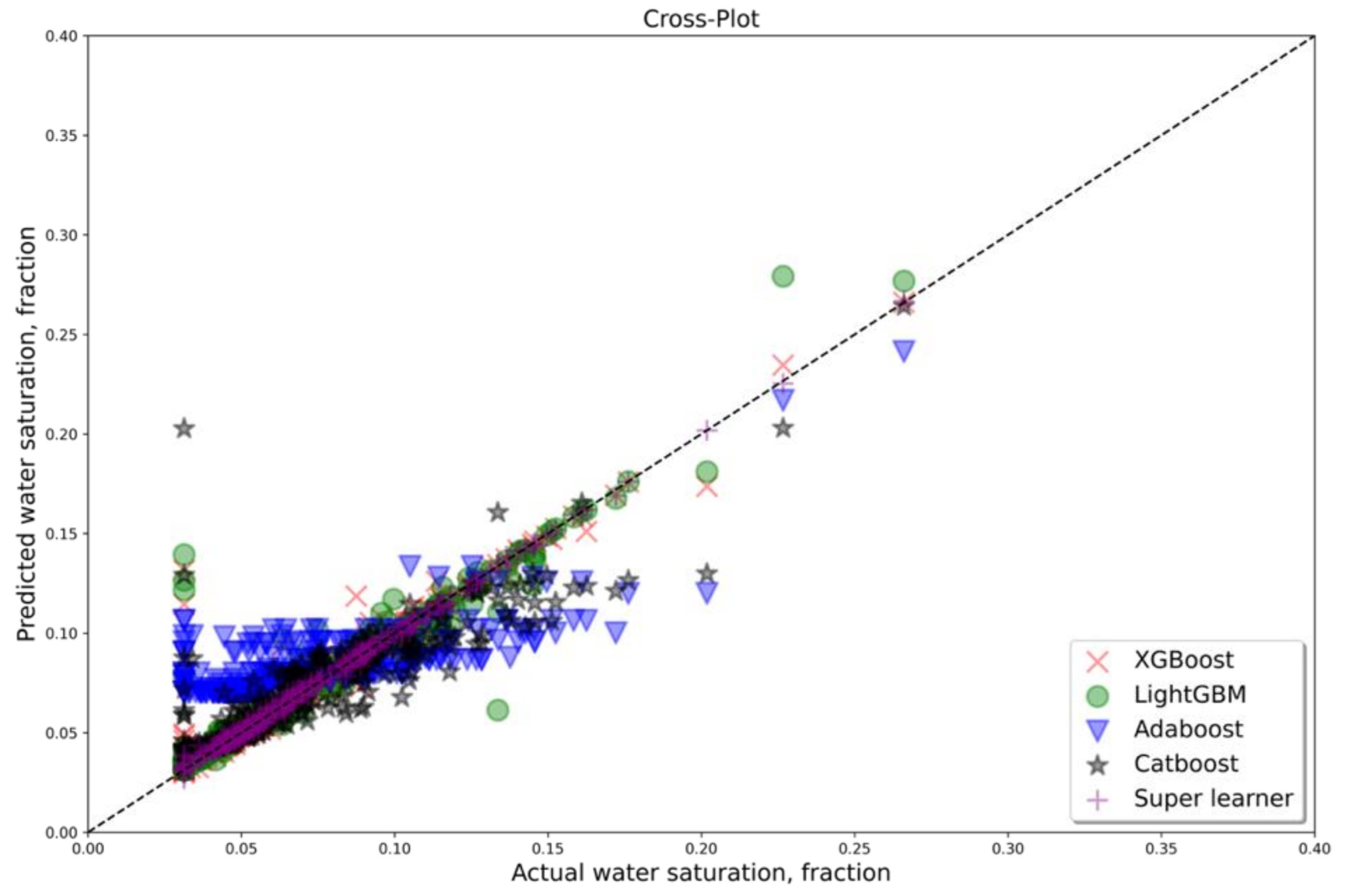
Appendix B. Cross Plots for All Wells, Which Were Considered as Testing for Dataset B with Four Features (PEF Excluded)

Figure A4. Cross plot for water saturation prediction results by different algorithms (Well 1).
Jmse 09 00666 g0a4
Figure A5. Cross plot for water saturation prediction results by different algorithms (Well 2).
Jmse 09 00666 g0a5
Figure A6. Cross plot for water saturation prediction results by different algorithms (Well 3).
Jmse 09 00666 g0a6

References

  1. Moradzadeh, A.; Bakhtiari, M.R. Methods of water saturation estimation: Historical perspective. J. Pet. Gas Eng. 2011, 3, 45–53. [Google Scholar]
  2. Awolayo, A.; Ashqar, A.; Uchida, M.; Salahuddin, A.A.; Olayiwola, S.O. A cohesive approach at estimating water saturation in a low-resistivity pay carbonate reservoir and its validation. J. Pet. Explor. Prod. Technol. 2017, 7, 637–657. [Google Scholar] [CrossRef] [Green Version]
  3. Archie, G.E. The Electrical Resistivity Log as an Aid in Determining Some Reservoir Characteristics. Trans. AIME 1942, 146, 54–62. [Google Scholar] [CrossRef]
  4. Archie, G.E. Electrical Resistivity an Aid in Core-Analysis Interpretation. AAPG Bull. 1947, 31, 350–366. [Google Scholar] [CrossRef]
  5. Archie, G.E. Introduction to Petrophysics of Reservoir Rocks. AAPG Bull. 1950, 34, 943–961. [Google Scholar] [CrossRef]
  6. Archie, G.E. Classification of carbonate reservoir rocks and petrophysical considerations. Aapg Bull. 1952, 36, 278–298. [Google Scholar]
  7. Shao, W.; Chen, S.; Eid, M.; Hursan, G. Carbonate log interpretation models based on machine learning techniques. In Proceedings of the SPWLA 60th Annual Logging Symposium, The Woodlands, TX, USA, 15–19 June 2019. [Google Scholar] [CrossRef]
  8. Bukar, I.; Adamu, M.B.; Hassan, U. A machine learning approach to shear sonic log prediction. In Proceedings of the SPE Nigeria Annual International Conference and Exhibition, Lagos, Nigeria, 5 August 2019. [Google Scholar]
  9. Anifowose, F.; Ewenla, A.O.; Eludiora, S.I. Prediction of Oil and Gas Reservoir Properties using Support Vector Machines. In Proceedings of the IPTC 2012: International Petroleum Technology Conference, Bangkok, Thailand, 7–9 February 2012; p. cp-280. [Google Scholar]
  10. Fattahi, H.; Karimpouli, S. Prediction of porosity and water saturation using pre-stack seismic attributes: A comparison of Bayesian inversion and computational intelligence methods. Comput. Geosci. 2016, 20, 1075–1094. [Google Scholar] [CrossRef]
  11. Mardi, M.; Ghasemalaskari, M.K. Application of Artificial Neural Networks in Water Saturation Prediction in from Iranian Oil Field. In Proceedings of the GeoBaikal 2010—First International Scientific and Practical Conference, Irkutsk, Russia, 15–20 August 2010; p. cp-248. [Google Scholar]
  12. Hamada, G.M.; Elshafei, M.A.; Adernian, A.M. Functional Network Softsensor for Determination of Porosity and Water Saturation in Sandstone Reservoirs. In Proceedings of the 72nd EAGE Conference and Exhibition incorporating SPE EUROPEC 2010, Barcelona, Spain, 14–17 June 2010; p. cp-161. [Google Scholar]
  13. Movahhed, A.; Bidhendi, M.N.; Masihi, M.; Emamzadeh, A. Introducing a method for calculating water saturation in a carbonate gas reservoir. J. Nat. Gas Sci. Eng. 2019, 70, 102942. [Google Scholar] [CrossRef]
  14. Mohammadi, A. Determination of Stone Groups of Asmari Formation Reservoir Based on Petrophysical Logs Using Fuzzy Logic Method. Master’s Thesis, University Tehran, Tehran, Iran, 2004. [Google Scholar]
  15. Sheremetov, L.; Martinez-Munoz, J.; Chi-Chim, M. Soft-computing method-ology for prediction of water saturation in fractured carbonate reservoirs. In Proceedings of the 80th EAGE Conference and Exhibition 2018, Copenhagen, Denmark, 11–14 June 2018; pp. 1–5. [Google Scholar]
  16. Negara, A.; Jin, G.; Agrawal, G. Enhancing rock property prediction from conventional well logs using machine learning technique-case studies of conventional and unconventional reservoirs. In Proceedings of the Abu Dhabi International Petroleum Exhibition & Conference, Abu Dhabi, United Arab Emirates, 7–10 November 2016. [Google Scholar]
  17. Eriavbe, F.E.; Okene, U.O. Machine learning application to permeability prediction using log & core measurements: A realistic work ow application for reservoir characterization. In Proceedings of the SPE Nigeria Annual International Conference and Exhibition, Lagos, Nigeria, 5–7 August 2019. [Google Scholar]
  18. Al-Bulushi, N.; King, P.; Blunt, M.; Kraaijveld, M. Development of artificial neural network models for predicting water saturation and fluid distribution. J. Pet. Sci. Eng. 2009, 68, 197–208. [Google Scholar] [CrossRef]
  19. Saumya, S.; Naqeeb, I.; Vij, J.; Khambra, I.; Kumar, A. Saturation Forecast Using Machine Learning: Enabling Smarter Decision-Making Capabilities. In Proceedings of the Abu Dhabi International Petroleum Exhibition & Conference, Society of Petroleum Engineers, Abu Dhabi, United Arab Emirates, 12 November 2019. [Google Scholar]
  20. Mollajan, A.; Memarian, H. Estimation of water saturation from petrophysical logs using radial basis function neural network. J. Tethys 2013, 1, 156–163. [Google Scholar]
  21. Gholanlo, H.H.; Amirpour, M.; Ahmadi, S. Estimation of water saturation by using radial based function artificial neural network in carbonate reservoir: A case study in Sarvak formation. Petroleum 2016, 2, 166–170. [Google Scholar] [CrossRef] [Green Version]
  22. Aliouane, L.; Ouadfeul, S.-A.; Djarfour, N.; Boudella, A. Petrophysical parameters estimation from well-logs data using multi-layer perceptron and radial basis function neural networks. In Proceedings of the International Conference on Neural Information Processing, Doha, Qatar, 12–15 November 2012; Springer: Berlin/Heidelberg, Germany, 2012; pp. 730–736. [Google Scholar]
  23. Masoudi, P.; Araabi, B.; Fa, T.A.; Memarian, H. Clustering as an efficient tool for assessing fluid content and movability by re-sistivity logs. In Proceedings of the Fourth International Mine and Mining Industries Congress & the Sixth Iranian Mining Engineering Conference, Tehran, Iran, October 2016. [Google Scholar]
  24. Mollajan, A. Application of local linear neuro-fuzzy model in estimating reservoir water saturation from well logs. Arab. J. Geosci. 2015, 8, 4863–4872. [Google Scholar] [CrossRef]
  25. Kapoor, G. Estimating Pore Fluid Saturation in an Oil Sands Reservoir Using Ensemble Tree Machine Learning Algorithms. Bachelor’s Thesis, Saint Mary’s University, Halifax, NS, Canada, 2017. [Google Scholar]
  26. Baziar, S.; Shahripour, H.B.; Tadayoni, M.; Nabi-Bidhendi, M. Prediction of water saturation in a tight gas sandstone reservoir by using four intelligent methods: A comparative study. Neural Comput. Appl. 2016, 30, 1171–1185. [Google Scholar] [CrossRef]
  27. Miah, M.I.; Zendehboudi, S.; Ahmed, S. Log data-driven model and feature ranking for water saturation prediction using machine learning approach. J. Pet. Sci. Eng. 2020, 194, 107291. [Google Scholar] [CrossRef]
  28. Kenari, S.A.J.; Mashohor, S. Robust committee machine for water saturation prediction. J. Pet. Sci. Eng. 2013, 104, 1–10. [Google Scholar] [CrossRef]
  29. Al-Amri, M.; Mahmoud, M.; Elkatatny, S.; Al-Yousef, H.; Al-Ghamdi, T. Integrated petrophysical and reservoir characterization work ow to enhance permeability and water saturation prediction. J. Afr. Earth Sci. 2017, 131, 105–116. [Google Scholar] [CrossRef] [Green Version]
  30. Kamalyar, K. Using Artificial Neural Network for Predicting Water Saturation in an Iranian Oil Reservoir. In Proceedings of the 10th EAGE International Conference on Geoinformatics-Theoretical and Applied Aspects, Kyiv, Ukraine, 10–14 May 2011; p. cp-240. [Google Scholar] [CrossRef]
  31. Friedman, J.H. Greedy function approximation: A gradient boosting ma-chine. Ann. Stat. 2001, 29, 1189–1232. [Google Scholar] [CrossRef]
  32. Ganatra, A.P.; Kosta, Y.P. Comprehensive Evolution and Evaluation of Boosting. Int. J. Comput. Theory Eng. 2010, 2, 931–936. [Google Scholar] [CrossRef]
  33. Snieder, E.; Khan, U.T. A comprehensive evaluation of boosting algorithms for artificial neural network-based ow forecasting models. In Proceedings of the AGU Fall Meeting 2019, San Francisco, CA, USA, 9–13 December 2019. [Google Scholar]
  34. Gonzalez-Recio, O.; Jiménez-Montero, J.; Alenda, R. The gradient boosting algorithm and random boosting for genome-assisted evaluation in large data sets. J. Dairy Sci. 2013, 96, 614–624. [Google Scholar] [CrossRef] [Green Version]
  35. Deconinck, E.; Zhang, M.H.; Coomans, D.; Heyden, Y.V. Evaluation of boosted regression trees (brts) and two-step brt pro-cedures to model and predict blood-brain barrier passage. J. Chemom. 2007, 21, 280–291. [Google Scholar] [CrossRef]
  36. Ray, S. Quick Introduction to Boosting Algorithms in Machine Learning. Available online: https://www.analyticsvidhya.com/blog/2015/11/quick-introduction-boosting-algorithms-machine-learning/ (accessed on 1 January 2019).
  37. Freung, Y.; Shapire, R. A decision-theoretic generalization of on-line learning and an application to boosting. J. Comput. Syst. Sci. 1997, 55, 119–139. [Google Scholar] [CrossRef] [Green Version]
  38. Freund, Y.; Schapire, R.; Abe, N. A short introduction to boosting. J. Jpn. Soc. Artif. Intell. 1999, 14, 1612. [Google Scholar]
  39. Chen, T.; Guestrin, C. XGboost: A scalable tree boosting system. In Proceedings of the 22nd ACM Sigkdd International Conference on Knowledge Discovery and Data Mining, San Francisco, CA, USA, 13–17 August 2016; pp. 785–794. [Google Scholar]
  40. Prokhorenkova, L.; Gusev, G.; Vorobev, A.; Dorogush, A.V.; Gulin, A. Cat-Boost: Unbiased Boosting with Categorical Features. In Proceedings of the Advances in Neural Information Processing Systems, Montreal, QC, Canada, 3–8 December 2018; pp. 663–6648. [Google Scholar]
  41. Prokhorenkova, L.; Gusev, G.; Vorobev, A.; Dorogush, A.V.; Gulin, A. CatBoost: Unbiased boosting with categorical features. arXiv 2017, preprint. arXiv:1706.09516. [Google Scholar]
  42. Al-Mudhafar, W.J. Integrating machine learning and data analytics for geostatistical characterization of clastic reservoirs. J. Pet. Sci. Eng. 2020, 195, 107837. [Google Scholar] [CrossRef]
  43. Subasi, A.; El-Amin, M.F.; Darwich, T.; Dossary, M. Permeability prediction of petroleum reservoirs using stochastic gradient boosting regression. J. Ambient. Intell. Humaniz. Comput. 2020, 1–10. [Google Scholar] [CrossRef]
  44. Erofeev, A.; Orlov, D.; Ryzhov, A.; Koroteev, D. Prediction of Porosity and Permeability Alteration Based on Machine Learning Algorithms. Transp. Porous Media 2019, 128, 677–700. [Google Scholar] [CrossRef] [Green Version]
  45. Zhang, L.; Zhan, C. Machine Learning in Rock Facies Classification: An Application of XGBoost. In Proceedings of the SEG Global Meeting Abstracts, Al Ain, United Arab Emirates, 9–12 October 2017; pp. 1371–1374. [Google Scholar] [CrossRef]
  46. Al-Mudhafar, W.; Jaber, A.K.; Al-Mudhafar, A. Integrating Probabilistic Neural Networks and Generalized Boosted Regression Modeling for Lithofacies Classification and Formation Permeability Estimation. In Proceedings of the OTC-27067-MS, the Offshore Technology Conference, Houston, TX, USA, 2–5 May 2016. [Google Scholar]
  47. Nielsen, D. Tree Boosting with Xgboost-Why Does Xgboost win “every” Machine Learning Competition? Master’s Thesis, NTNU, Trondheim, Norway, 2016. [Google Scholar]
  48. Van der Laan, M.J.; Polley, E.C.; Hubbard, A.E. Super Learner. U.C. Berkeley Division of Biostatistics Working Paper Series. 2014. Available online: Bepress.com/ucbbiostat/paper222 (accessed on 1 November 2007).
  49. Polley, E.C.; van der Laan, M.J. “Super Learner In Prediction”. U.C. Berkeley Division of Biostatistics Working Paper Series. Working Paper 266. 2010. Available online: https://biostats.bepress.com/ucbbiostat/paper266 (accessed on 1 January 2019).
  50. Amyx, J.; Bass, D.; Whiting, R.L. Petroleum Reservoir Engineering Physical Properties; McGraw-Hill: New York, NY, USA, 1960. [Google Scholar]
  51. Rokach, L. Decision forest: Twenty years of research. Inf. Fusion 2016, 27, 111–125. [Google Scholar] [CrossRef]
  52. Hastie, T.; Rosset, S.; Zhu, J.; Zou, H. Multi-class AdaBoost. Stat. Its Interface 2009, 2, 349–360. [Google Scholar] [CrossRef] [Green Version]
  53. Tahmasebi, P.; Kamrava, S.; Bai, T.; Sahimi, M. Machine learning in geo-and environmental sciences: From small to large scale. Adv. Water Resour. 2020, 103619. [Google Scholar]
  54. Ke, G.; Meng, Q.; Finley, T.; Wang, T.; Chen, W.; Ma, W.; Ye, Q.; Liu, T. LightGBM: A Highly Efficient Gradient Boosting Decision Tree. Advances in Neural Information Processing Systems 30 (NIPS 2017). Available online: https://papers.nips.cc/paper/2017 (accessed on 1 January 2019).
  55. Gibert, K.; Sànchez-Marrè, M.; Izquierdo, J. A survey on pre-processing techniques: Relevant issues in the context of environmental data mining. AI Commun. 2016, 29, 627–663. [Google Scholar] [CrossRef] [Green Version]
  56. Sen, M. Srivastava, Regression Analysis: Theory, Methods, and Applications; Springer Science & Business Media: Berlin/Heidelberg, Germany, 2012. [Google Scholar]
  57. Layton, R. Learning Data Mining with Python; Packt Publishing Ltd.: Birmingham, UK, 2015. [Google Scholar]
  58. Massaron, L.; Boschetti, A. Regression Analysis with Python; Packt Publishing Ltd.: Birmingham, UK, 2016. [Google Scholar]
Figure 1. Schematic of K-fold cross-validation.
Jmse 09 00666 g001
Figure 2. The schematic flowchart for building the ML models.
Jmse 09 00666 g002
Figure 3. Petrophysical well log data from a representative well in the study area. From left to right, track 1 represents gamma ray, track 2 represents bulk density log in red, neutron density in blue, sonic log in black and photoelectronic log in purple. Track 3 represents deep and shallow, resistivity logs in red and blue, respectively. These logs are the input for the proposed models to predict water saturation as shown in Track 4 through the following parameters for the Archie equation: m = 1.49; n = 1.82; a = 1.532; Rw = 0.35. blue dots in Track 4, are experimentally measured water saturation in the lab and red line is predicted water saturation by Archie’s equation.
Jmse 09 00666 g003
Figure 4. XGboost level-wise tree growth representation.
Jmse 09 00666 g004
Figure 5. Superlearner flowchart.
Jmse 09 00666 g005
Figure 6. Cross-plot of water saturation prediction results by different algorithms for dataset A, which depicts well log data-lab verified values vs. algorithm based ones, (A) XGBoost, (B) LightGBM, (C) Adaboost, (D) Catboost and (E) Super lerner.
Jmse 09 00666 g006aJmse 09 00666 g006b
Figure 7. Evaluation metrics for dataset A comparing among various methods. It is observed that Super Learner performs the best.
Jmse 09 00666 g007
Figure 8. Water saturation well log prediction results by different algorithms for one representative well from dataset A. In this figure, the red curve represents predicted values, and the black line is target values. It is seen that a perfect match is obtained via Super Learner method.
Jmse 09 00666 g008
Figure 9. Evaluation metrics for dataset B where PEF log has not been used for analysis in the algorithms where it’s found that Super Learner is generating best results compared to other methods.
Jmse 09 00666 g009
Figure 10. Cross plot for water saturation prediction results by different algorithms for dataset B. Cross-plots are representing target values vs. the predicted values. Here, PEF log has not been used as an input parameter and it is observed that super leaner still is generating the best results, (A) XGBoost, (B) LightGBM, (C) Adaboost, (D) Catboost and (E) Superlerner.
Jmse 09 00666 g010aJmse 09 00666 g010b
Figure 11. Water saturation prediction results by different algorithms for one well from dataset B where PEF log is kept out, and a perfect match between predictions and Archie-based calculated values are obtained via Super Learner method. In this image, the red line represents predicted values, and the black line is Archie measured ones but verified by experimental tests.
Jmse 09 00666 g011
Figure 12. The estimated score for potential input parameters. It can be seen that PEF has the lowest importance compared to all other well logs.
Jmse 09 00666 g012
Table 1. Machine learning Algorithms and their packages.
Algorithms Python PackagePackage VersionWebsite of the Package
XGBoostxgboost0.9.0https://xgboost.readthedocs.io/en/latest/index.html
Lightgbmlightgbm2.3.2https://lightgbm.readthedocs.io/en/
AdaboostAdaboost0.23.1https://scikit-learn.org
CatboostCatboost0.4https://catboost.ai
Random Forestscikit-learn0.22.2https://scikit-learn.org/dev/index.html
Super learnermlens0.1http://ml-ensemble.com
date accessed: January 2019–June 2020.
Table 2. Lists the boosting algorithms applied in our work, the tuned hyperparameter search interval, and the optimal hyperparameter values. For typical hyperparameters, we have used a common search interval that can lead to meaningful insights by comparison.
AlgorithmsHyperparameters TunedSearch IntervalOptimal Values
XGBoostLearning_rate
Subsample
Colsample_bytree
max_depth
n_estimators
0.01–0.5
0.5–1
0.5–1
1–14
1000–4000
0.1
0.8
0.8
9
3000
LightGBMlearning_rate
num_leaves
max_depth
n_estimators
0.01–0.5
3–95
1–14
1000–3000
0.1
70
7
2000
AdaboostLearning_rate
n_estimators
0.01–0.2
1500–3000
0.05
1600
CatboostLearning_rate
depth
iterations
0.01–0.4
1–14
1500–3000
0.1
7
1800
Table 3. Evaluation metrics summary for dataset A.
AlgorithmR2RMSEMAEMSE
TrainingTestingTrainingTestingTrainingTestingTrainingTesting
XGBoost0.9975790.993250.0097500.0099340.0071790.00783570.0000950.000102
LightGBM0.9248100.9189420.0329300.0359760.0109990.0113050.0010840.001294
Adaboost0.8866840.8666330.0624330.0519070.0403700.0508340.0038970.005236
Catboost0.9577580.9413680.0264220.0529270.0043810.0359120.0006980.002801
Super learner0.9988280.9972450.0095910.0104000.0015670.0076860.0000920.000108
Table 4. Evaluation metrics summary for dataset B where PEF log is kept out of the analysis/predictions.
AlgorithmR2RMSEMAEMSE
TrainingTestingTrainingTestingTrainingTestingTrainingTesting
XGBoost0.994810.9934820.0081640.0085400.0029210.0032030.0000660.000073
LightGBM0.983910.9829040.0130470.0138320.0039130.0047550.0001720.000191
Adaboost0.942610.9329930.0269520.0273840.0198230.0229120.0007260.000750
Catboost0.939120.9319260.0270910.0276010.0118920.0122720.0007330.000762
Super Learner0.999890.9997270.0017110.0017480.0011970.0012300.00000290.000003
Table 5. The computational cost for the algorithms used in this study.
AlgorithmsXGboostAdaboostSuperlearner CatboostLightgbm
Run Time (s)530.462322.011466.198630.198301.622
Publisher’s Note: MDPI stays neutral with regard to jurisdictional claims in published maps and institutional affiliations.

