Fault Detection Based on Fully Convolutional Networks (FCN)

Abstract

It is of great significance to detect faults correctly in continental sandstone reservoirs in the east of China to understand the distribution of remaining structural reservoirs for more efficient development operation. However, the majority of the faults is characterized by small displacements and unclear components, which makes it hard to recognize them in seismic data via traditional methods. We consider fault detection as an end-to-end binary image-segmentation problem of labeling a 3D seismic image with ones as faults and zeros elsewhere. Thus, we developed a fully convolutional network (FCN) based method to fault segmentation and used the synthetic seismic data to generate an accurate and sufficient training data set. The architecture of FCN is a modified version of the VGGNet (A convolutional neural network was named by Visual Geometry Group). Transforming fully connected layers into convolution layers enables a classification net to create a heatmap. Adding the deconvolution layers produces an efficient network for end-to-end dense learning. Herein, we took advantage of the fact that a fault binary image is highly biased with mostly zeros but only very limited ones on the faults. A balanced crossentropy loss function was defined to adjust the imbalance for optimizing the parameters of our FCN model. Ultimately, the FCN model was applied on real field data to propose that our FCN model can outperform conventional methods in fault predictions from seismic images in a more accurate and efficient manner.

1. Introduction

In both unconventional and conventional reservoirs in eastern China, faults play a major role in lateral sealing of thin reservoirs and controlling the accumulation of the remaining oil [1,2,3]. Almost all of the developed oil and gas fields in eastern China are distributed in rift basins which are rich in oil and gas resources with highly developed and very complex fault systems [4,5,6]. Based on current theories and techniques, significant difficulties still exist in the accurate identification and characterization of faults. This is because a variety of faults can be developed in rift basins, such as normal faults, normal oblique-slip faults, oblique faults, and strike-slip faults, with different combinations of planes and sections, most of which are broom shaped, comb shaped, goose row shaped, and parallel interlaced in planes. In this regard, most of them are Y-shaped and negative flower shaped in sections [7,8]. In a rift basin, the filling of sediments, the development and distribution of sedimentary sequences, the formation, distribution, and evolution of oil and gas pools (including the formation and effectiveness of traps, hydrocarbon migration, and accumulation) are closely related to the distribution and activities of faults [9,10]. Therefore, fine detection and characterization of faults in rift basins in eastern China has become a key basic geological problem for oil and gas exploration and development efforts and has become the key topic of basin tectonic research.

The basic fault detection attempt is done by manually interpreting 3D seismic data and picking horizons. This method relies heavily on the experience and regional geology knowledge of the interpreter, which is not efficient and has proven to be erroneous. With the rapid development of seismic attributes, a number of fault detection methods have emerged at home and abroad, such as semblance [11], coherency [12,13,14], variance [15,16], and gradient magnitude [17]. These methods recognize faults as lateral reflection discontinuities in a 3D seismic image. These seismic attributes, however, can be sensitive to noise and stratigraphic features, which also correspond to discontinuities in the reflector in a seismic profile. This means that measuring seismic reflection continuity or discontinuity alone is insufficient to detect faults [18]. In recent years, a growing number of scholars are adopting deep learning in seismic interpretation and fault recognition in the realm of artificial intelligence (AI). In order to perform fault detection, several convolutional-neural-network (CNN) methods have been introduced that are based on pixel-wise fault classification (fault or nonfault) with multiple seismic attributes [19,20,21,22,23,24,25,26,27]. Training and validation of a CNN model often requires a large number of seismic images and corresponding labels. Although there is applicability, manually labeling or interpreting faults in a 3D seismic image could be extremely time consuming and highly subjective. In addition, inaccurate manual interpretation, including mislabeled and unlabeled faults, may mislead the learning process [28].

In this paper, we consider the fault detection process as a more efficient end-to-end binary image-segmentation problem by using a new network. Image segmentation has been well studied in computer science, and multiple powerful CNN architectures [29,30,31,32,33,34] have been proposed to obtain superior segmentation results. Unlike traditional CNN with input layer, convolution layer, pooling layer, fully connected layer, output layer and other auxiliary layers, as main constituent components, the fully convolutional networks (FCN) does not have any fully connected layer, with a convolutional layer, pooling layer, and deconvolutional layer as its core [35]. FCN can achieve pixel-wise classification by semantic segmentation of the entire data in the image, which significantly improves the computational efficiency and precision of the algorithm.

In this study, we developed a FCN-based method to automatically detect faults. The architecture of FCN is a modified version of the VGGNet (A convolutional neural network was developed by the University of Oxford's Visual Geometry Group and Google DeepMind in 2014) whereby the fully connected layers has been replaced by the fully convolutional layers with the addition of deconvolutional layers. Considering that a fault binary image is highly biased with mostly zeros and very limited ones on the faults, we utilized a balanced crossentropy loss function to optimize the parameters of our FCN model. To train and validate our FCN model, we propose an effective and efficient way to automatically generate synthetic seismic images and corresponding fault labels. Moreover, we trained and validated the neural network using 300 and 30 pairs of synthetic seismic and fault images, respectively. By using a NVIDIA’s TITAN Xp graphics processing unit (GPU), our FCN model takes about 35 min to predict faults in a large field data volume with 500 × 550 × 2000 samples.

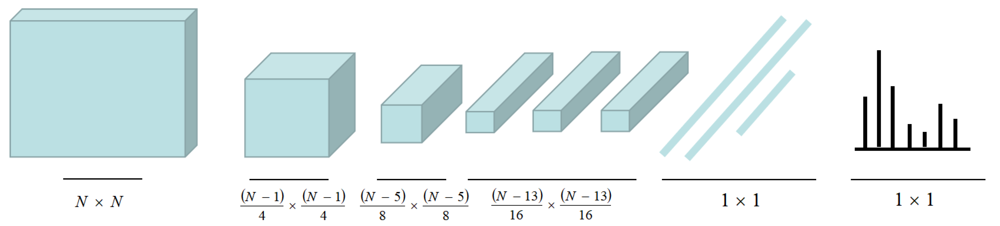
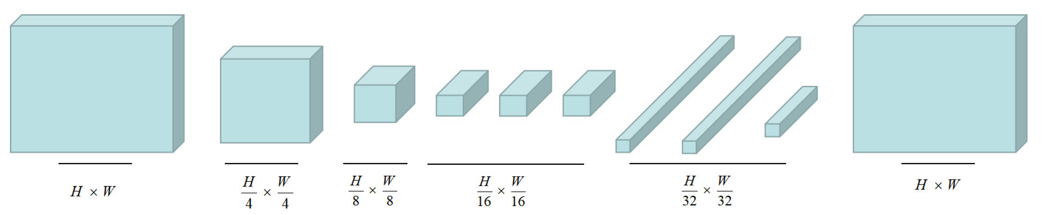
2. Illustration of FCN

CNN has achieved great success in the field of image classification, and several network models such as VGGNet and AlexNet [36] have emerged as a result. Due to its multi-layer structure, it can learn features automatically, with multiple levels of features. For example, the shallow convolution layer has a small perception domain, and it can learn some local features, whereas the deeper convolution layer has a larger perception domain and it can learn more abstract features. Because these abstract features are less sensitive to the size, position, and direction of the object, CNN cannot precisely recognize the outlines of an object and its corresponding pixels, though they are highly capable of improving the classification performance and can distinguish the types of objects in an image. Far from image classification, FCN is proposed for image segmentation, which has become the basic framework of semantic segmentation [2,35,37,38,39]. For conventional CNN, as shown in Figure 1, some fully connected layers will be added at the end of the network to obtain 1D category probability information. This probability information can only identify the category of the whole image, not the category of each pixel. In FCN, transforming fully connected layers into convolution layers enables a classification net to output a heatmap. As shown in Figure 2, FCN is an end-to-end, pixel-to-pixel network.

The typical architecture of the FCN is shown in Figure 3. The core component of FCN is the convolutional layer, which is mainly responsible for feature learning. It contains several feature maps processed by the convolution kernels. Each convolution kernel processes data solely for its receptive field with the same shared weights, thus reducing the number of free parameters and allowing FCN to be deeper with fewer parameters. The formula for calculating the convolutional layers is as follows:

$$conv(i,j)=R\left({\displaystyle \sum _{u=0}^{M-1}{\displaystyle \sum _{v=0}^{M-1}{w}_{u,v}{x}_{i+u,j+v}+b}}\right)$$

(1)

where $conv(i,j)$ is the convolution result, also known as the feature map; M indicates the size of the convolution kernel (M × M); $w_{u,v}$ is the weight of the convolution kernel in line $u$ and column $v$; $x_{i+u,j+v}$ is the input; $b$ is the bias; and $R$ is the activation function, which brings a nonlinear factor that allows FCN to approximate any nonlinear function.

The rectified linear unit (ReLU) function [40] is used as the activation function in most neural networks. The ReLU function can be expressed as R(x) = max(0, x), which helps save computational cost, reduce the vanishing gradient problem, and alleviate overfitting.

The pooling layer follows the convolutional layers, which is used for nonlinear down-sampling. The pooling layer can reduce the number of dimensions and parameters by combining the outputs of the neuron clusters into a single neuron. The pooling layer can be performed in two separate approaches: average pooling and max pooling. Average pooling uses the average value from the feature maps at the prior layer, whereas the max pooling takes advantage of the maximum value. In modern networks, max pooling has often been used [41] and can be expressed as

$$R_{u,v}=\underset{i\in D_{u,v}}{\max }(x_i)$$

(2)

where $x_i$ is the value of each neuron in the region $D_{u,v}$ and $R_{u,v}$ is the value after max pooling.

In CNN, the convolution layer is closely followed by the FC layers. The FC layers connect every neuron to all former layers, and the flattened matrix goes through the FC layer to get a dense prediction, which is used to classify the images. However, FCN replaces these FC layers with fully convolutional layers.

Through previous multiple convolution operations, we obtained the final feature map. On this basis, multiple up-sampling operations are carried out to make the output result consistent with the input size, thus obtaining the pixel-level prediction result. We often use deconvolution to up-sample. On the contrary, deconvolution is the inverse process of convolution, which is also called transposed convolution. In the convolution process, the pooling layers make the feature map smaller and smaller, and a lot of useful information will be lost. If we perform up-sampling directly with deconvolution, the prediction results will be very rough. Therefore, we build a novel skip architecture and crop useful feature information to refine prediction [35]. Through the skip architecture, the detailed features of the lower layers can be fused with those of the deep layers. Combining fine layers and coarse layers allows the model to make local predictions that at the same time will respect the global structure.

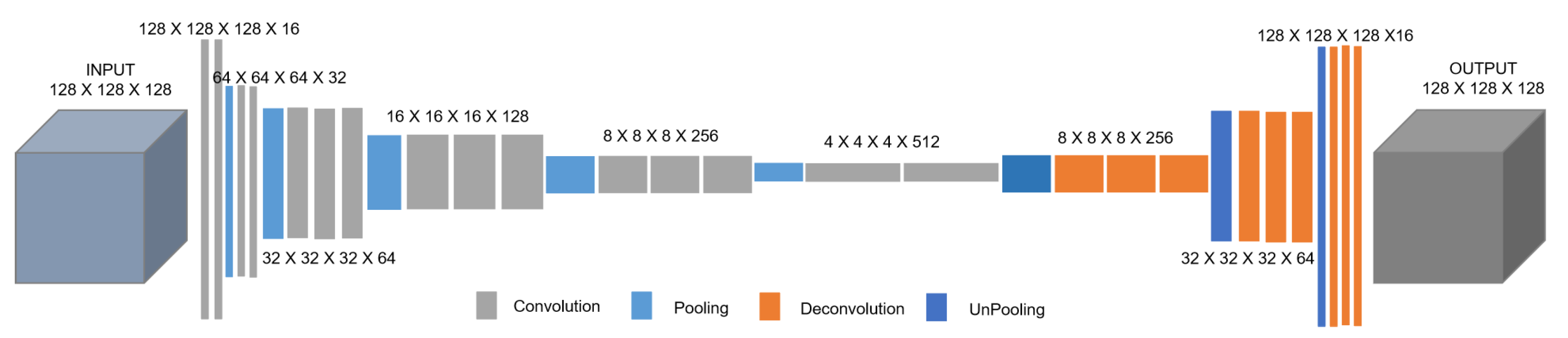
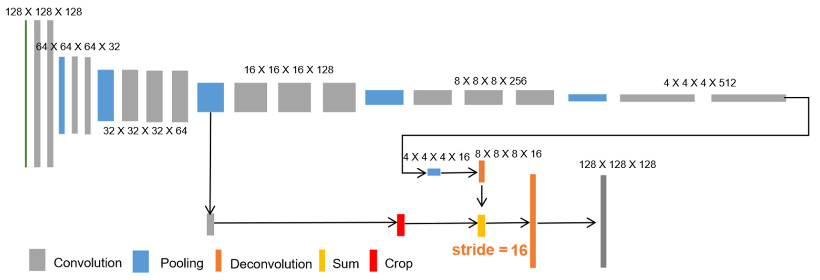
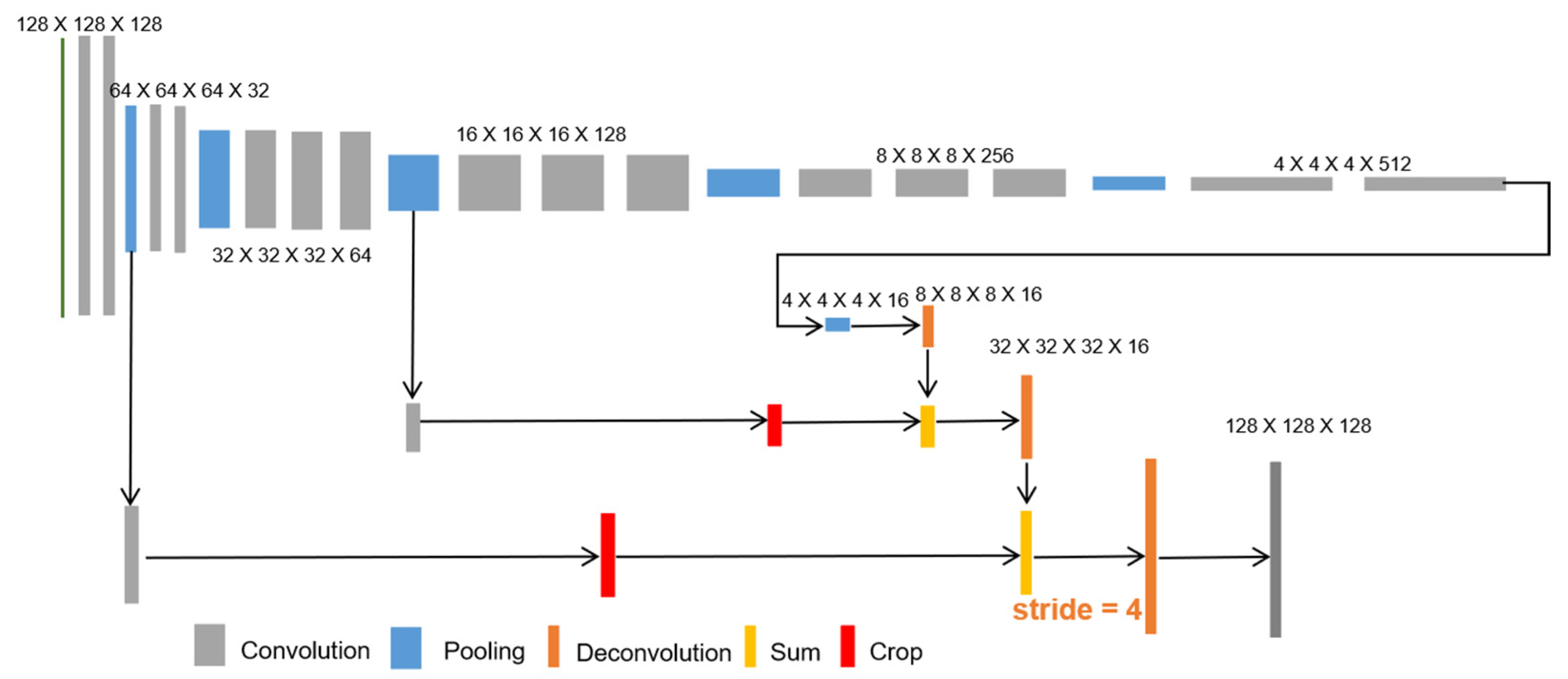
3. Architecture of Our FCN

The proposed FCN is established by modifying the VGGNet, which is one of the CNN networks. The training time required for the VGGNet is significantly less than required for AlexNet [40]. A variety of architectures of the VGGNet exist because of different number of layers. Figure 4 shows the commonly used architecture VGG16.

We take the VGG16 as the foundation for our network. Figure 5 displays the architecture of our FCN. First, we changed the input dimensions to 128 × 128 × 128, which is the size of the 3D seismic image. Moreover, we replace FC layers with fully convolutional layers and add deconvolution layers behind it. In the convolution part, each step contains some 3 × 3 × 3 convolutional layers followed by a ReLU activation and a 2 × 2 × 2 max pooling operation with stride 2 for down-sampling. In the deconvolution part, every step contains three 3 × 3 × 3 deconvolutional layers and a 2 × 2 × 2 max unpooling layer.

The output of our FCN is the fault probability body, where 1 represents fault and 0 represents nonfault. Because the initial value of the weight in the convolution layer is random, there will be a deviation between the prediction and the actual in the early stage of neural network training; therefore, it is necessary to use the random gradient descent algorithm to continuously update the value of the network parameters and reduce the value of the loss function. This should be done until the prediction and the actual response gradually converge. Because most of prediction results are nonfault, almost 90% of them are 0 values. We used the following balanced crossentropy loss function as discussed in [32] to achieve this goal:

$$L=-\beta {\displaystyle \sum _{i=0}^{i=N}{y}_i\log (p_i)-(1-\beta )}{\displaystyle \sum _{i=0}^{i=N}(1-y_i)\log (1-p_i)}$$

(3)

where $\beta =\frac{{\displaystyle {\sum }_{i=0}^{i=N}(1-y_i)}}{N}$ represents the ratio between nonfault pixels and the total image pixels, whereas $1-\beta$ denotes the ratio of fault pixels in the 3D seismic image. $p_i$ represents the probability of a fault, and $y_i$ is the label value.

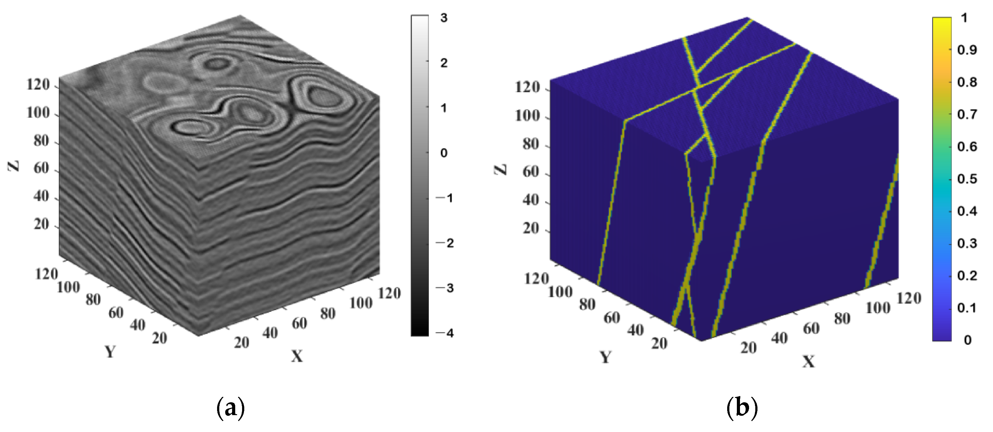
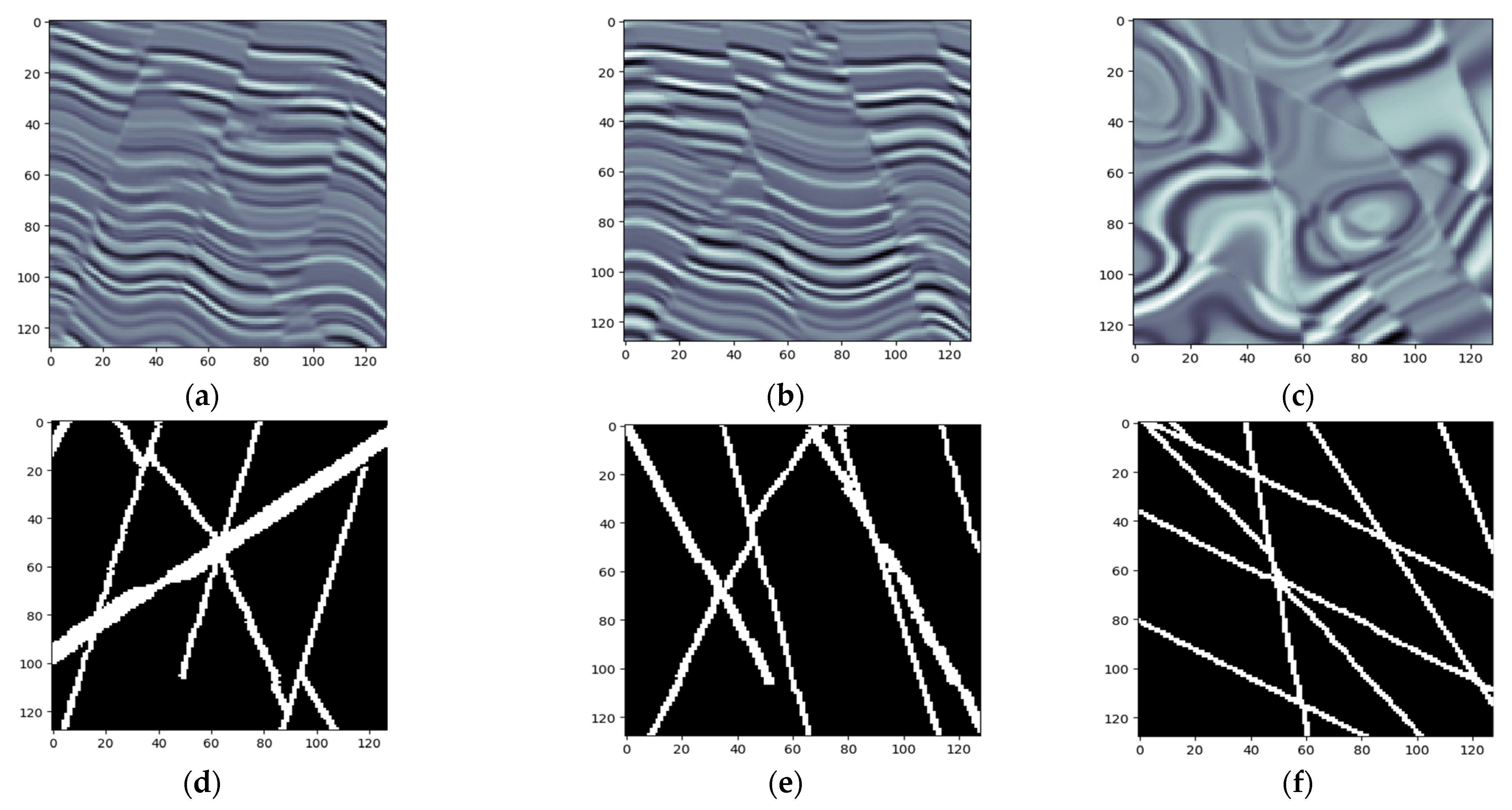
4. Synthesizing Seismic Data Sets

It is important to synthesize seismic data sets before training the neural network, which can provide sufficient training and validation data sets for our network. The synthetic seismic data sets are from open-source data sets [28], which are all automatically generated by randomly adding folding, faulting, and noise in the volumes. The simplified workflow to synthesize seismic data sets is performed as follows:

1)

The horizontal reflectivity model is designed as $h(x,y,z)$ with a sequence of random values that are in the range of [−1,1].

2)

Use Equation (4) to generate a fold structure.

$$f_1(x,y,z)=m_0-\frac{2.1z}{z_{\max }}{\displaystyle \underset{1}{\overset{n}{\mathrm{\int }}}{n}_k{e}^{\frac{{(x-l_k)}^2+{(y-p_k)}^2}{2{\sigma }_k^2}}}$$

(4)

which combines with multiple 2D Gaussian functions and a linear-scale function $2.1z/z_{\max }$. The combination of 2D Gaussian functions creates laterally varying folding structures, whereas the linear-scale function dampens the folding vertically from bottom to top. In this equation, each combination of the parameters $m_0,n_k,l_k,p_k,{\sigma }_k$ generates some specific spatially varying folding str uctures in the model. By randomly choosing each of the parameters from predefined ranges, we are able to create numerous models with unique structures.

3)

Substituting $f_1(x,y,z)$ into $h(x,y,z)$ leads to $h(x,y,z+f_1(x,y,z))$.

4)

Planar shearing of $h(x,y,z+f_1(x,y,z))$ through $f_2(x,y,z)=t_0+ix+jy$ leads to $h(x,y,z+f_1+f_2)$. In the model $h(x,y,z+f_1+f_2)$, the parameters $t_0,i,j$ are randomly chosen from some predefined ranges.

5)

Use Equation (5) to add planar faulting in the model $h(x,y,z+f_1+f_2)$ and create a reflectivity model containing folds and faults.

$$h_1(x,y,z)=h(x,y,z+f_1+f_2)e^{-\frac{1}{2}{z}^T{R}^T{S}^{T}Rz}$$

(5)

where

$$R=\left[\begin{array}{c}uf\\ vf\\ wf\end{array}\right],S=\left[\begin{array}{ccc}\frac{1}{{\sigma }_{uf}^2}& 0& 0\\ 0& \frac{1}{{\sigma }_{vf}^2}& 0\\ 0& 0& \frac{1}{{\sigma }_{wf}^2}\end{array}\right]$$

(6)

where $uf$ is the vector representing the dip angle of the fault, $vf$ is the vector representing the strike of the fault, and $wf$ is the vector representing the normal direction perpendicular to the strike of the fault. ${\sigma }_{uf}$, ${\sigma }_{vf}$, and ${\sigma }_{wf}$ respectively represent the distribution range of the fault in the direction of $uf$, $vf$, and $wf$.

6)

Convoluting the reflectivity model with a Ricker wavelet to obtain a 3D seismic image.

In order to construct a more realistic synthetic seismic image, some random noise is added. From this noisy image, we crop a final training seismic data set (Figure 6a) with the size of 128 × 128 × 128 to avoid the artifacts near the boundaries. Figure 6b illustrates the corresponding binary fault labeling data set, and Figure 7 depicts the faults on the synthetic training data set. Randomly selected vertical sections and time slices are inline 65, crossline 50, and time slice at 80 ms, respectively.

To generate sufficient training data to optimally train the neural network for fault segmentation, we randomly chose parameters of faulting, folding, wavelet peak frequency, and noise to obtain 300 pairs of 3D unique seismic images and corresponding fault labeling images by using this workflow. Using the same workflow, we also automatically generated 30 pairs of seismic and fault labeling images for the validation. To increase the diversity of the data sets and to prevent our FCN model from learning irrelevant patterns, we applied simple data augmentations including vertical flip and rotation around the vertical time or depth axis. When rotating the seismic and fault labeling volumes, we have six options of 45°, 90°, 135°, 180°, 225°, and 270°.

5. Training and Validation

We trained our FCN model by using 300 pairs of synthetic 3D seismic and fault images that are automatically created shown in Figure 6 and Figure 7. The validation data set contains another 30 pairs of such synthetic seismic and fault images, which are not used in the training data set. Prior to training, each image is subtracted by its mean value and divided by its standard deviation. This normalization is necessary because the amplitude values of different real seismic images can differ from one another. The training data sets are used to train a given model and optimize the parameters, whereas the validation data sets are used to evaluate a given model during the training process and prevent overfitting of the model. We fed the 3D seismic images to the FCN model in batches. Each batch contains seven images, which consist of an original image and its rotation around the vertical time/depth axis by 45°, 90°, 135°, 180°, 225°, and 270°. If adequate GPU memory is available, a larger batch size can be tried. We train the network with 30 epochs, and all the 300 training images are processed at each epoch.

To make up-sampling more detailed, we divide the training process into three stages where the deconvolution stride gets smaller at each stage. In the first stage, as shown in Figure 8, the deconvolution stride is 32. In the second stage, we carry out the training with stride 16, as presented in Figure 9. During this process, there are two deconvolution operations. Before the second deconvolution, we crop the prediction results of the third pooling layer. Next, deconvolution is applied to obtain the predicted results of 128 × 128 × 128 by using the skip architecture to sum the first deconvolution result and the cropped result. In the last stage, we perform the training with stride 4 with three deconvolution operations. Before the third deconvolution, the prediction results of the first pooling layer are cropped. Then, deconvolution with stride 4 is performed by employing the skip architecture to sum the second deconvolution result and the cropped result as shown in Figure 10. Considering Figure 11, the training and validation accuracies gradually increase to 95%, whereas the training and validation loss converges to 0.01 after 30 epochs.

6. Application

The trained FCN model is applied to automatic fault interpretation of a real field seismic data. The study area is located in an oil field in eastern China, where complicated faults are widely present in the target formation [42,43,44]. Above 1700 ms, faults appear, and most of them are Y-shaped in profiles. The fault features are more complex below 1700 ms, however, due to the extensive existence of igneous rocks in the Dongying Formation, the quality of seismic data is seriously deteriorated, and the accuracy of fault picking becomes poor and challenging. In the plane, the fault is affected by tensile and strike-slip stress regimes, and the fault strike is mainly NE and NW. This data set consists of 500 (lines) × 550 (CDPs) with a line spacing of 25 m and a CDP spacing of 25 m. The data are sampled at 1 ms with a length of 2 s. The inline number and xline number are in the range of [2400,2900] and [3600,4150], respectively. By using one NVIDIA’s TITAN Xp GPU, computing the FCN fault probability volume takes about 35 min. We compare our fault prediction results with the fault likelihood, which is somehow a reliable attribute for fault detection. A randomly selected vertical section and time slice are inline 2530 and time slice at 1500 ms, respectively. The results of the fault detection are displayed in Figure 12 and Figure 13.

Figure 12b presents the fault image predicted via the trained FCN model and Figure 12c, the fault-likelihood attribute. The fault likelihood (Figure 12c) is reliable enough to delineate the faults within this seismic image. However, the presence of other features (noise) is observed in the fault-likelihood image compared to the one predicted by the FCN (Figure 12b). In addition, the fault likelihood has picked an abundance of horizontal fault features (Figure 12c), which are geologically unrealistic. Figure 13b,c illustrates the fault detection results at different slices. We observed that most faults are clearly detected under the trained FCN model, and multiple sets of faults striking in different directions are distinguished on the horizontal slice. Figure 13c is the fault likelihood at the same slice, which were able to detect most of the faults, but the features are much noisier than the FCN fault slice.

In summary, the field data example demonstrates that the proposed FCN-based method has superior performance in detecting faults and provides relatively higher sensitivity and continuity with less noise. In addition, fault prediction using the trained FCN model is highly efficient compared to seismic attributes to detect faults for the same volume, when common normal workstations are being used.

7. Conclusions

We developed a FCN-based method to automatically detect faults in the continental sandstone reservoirs in the east of China. The architecture of FCN is a modified version of the VGGNet. We trained our FCN model by using only 300 pairs of 3D synthetic seismic and fault volumes, which were all automatically generated. Because the distribution of fault and non-fault samples was heavily biased, a balanced loss function to optimize the FCN model parameters was defined. In the network training process, we employed a skip architecture and a crop operation several times to improve the accuracy of prediction results. The practical application results confirmed that FCN outperforms automatic and common fault detection methods (attributes) and is highly noise proof for providing a sharp image of the faults even in a complex structure.

References

1. Liu, B.; Yan, D.; Fu, X.; Lü, Y.; Gong, L.; Wang, S. Investigation of geochemical characteristics of hydrocarbon gas and its implications for Late Miocene transpressional strength—A study in the Fangzheng Basin, Northeast China. Interpretation 2018, 6, T83–T96. [Google Scholar] [CrossRef] [Green Version]
2. Liu, B.; Zhao, X.; Fu, X.; Yuan, B.; Bai, L.; Zhang, Y.; Ostadhassan, M. Petrophysical characteristics and log identification of lacustrine shale lithofacies: A case study of the first member of Qingshankou Formation in the Songliao Basin, Northeast China. Interpretation 2020, 8, SL45–SL57. [Google Scholar] [CrossRef]
3. Liu, B.; Sun, J.; Zhang, Y.; He, J.; Fu, X.; Yang, L.; Xing, J.; Zhao, X. Reservoir space and enrichment model of shale oil in the first member of Cretaceous Qingshankou Formation in the Changling sag, southern Songliao Basin, NE China. Pet. Explor. Dev. 2021, 48, 1–16. [Google Scholar]
4. Xu, J. Similarities between Cenozoic basins of different magnitudes in East Asia continental margin. Pet. Geol. Exp. 1997, 19, 297–304. [Google Scholar]
5. Xu, J.; Zhang, L. Genesis of Cenozoic basins in Northwest Pacific Ocean margin(1): Comments on basin-forming mechanism. Oil Gas Geol. 2000, 21, 93–98. [Google Scholar]
6. Chen, W.-C.; Yan, J.-J. On the Evolutional Characteristics of Cenozoic Episodic rifting of Nanpu Sag. J. Jining Norm. Coll. 2020, 3, 115–119. [Google Scholar]
7. Peacock, D.C.P.; Sanderson, D.J.; Rotevatn, A. Relationships between fractures. J. Struct. Geol. 2018, 106, 41–53. [Google Scholar] [CrossRef]
8. Peacock, D.C.P.; Nixon, C.W.; Sanderson, A.R.D.J.; Zuluaga, L.F. Interacting faults. J. Struct. Geol. 2017, 97, 1–22. [Google Scholar] [CrossRef]
9. Tong, H.M.; Meng, L.J.; Cai, D.S.; Wu, Y.P.; Li, X.S.; Liu, M.Q. Fault formation and evolution in rift basins-sandbox modeling and cognition. Acta Geol. Sin. 2009, 83, 759–774. [Google Scholar]
10. Tong, H.; Zhao, B.; Cao, Z.; Liu, G.; Dun, X.M.; Zhao, D. Structural analysis of faulting system origin in the Nanpu sag, Bohai Bay basin. Acta Geol. Sin. 2013, 87, 1647–1661. [Google Scholar]
11. Marfurt, K.J.; Kirlin, R.L.; Farmer, S.L.; Bahorich, M.S. 3-D seismic attributes using a semblance-based coherency algorithm. Geophysics 1998, 63, 1150–1165. [Google Scholar] [CrossRef] [Green Version]
12. Marfurt, K.J.; Sudhaker, V.; Gersztenkorn, A.; Crawford, K.D.; Nissen, S.E. Coherency calculations in the presence of structural dip. Geophysics 1999, 64, 104–111. [Google Scholar] [CrossRef]
13. Li, F.; Lu, W. Coherence attribute at different spectral scales. Interpretation 2014, 2, SA99–SA106. [Google Scholar] [CrossRef] [Green Version]
14. Wu, X. Directional structure-tensor based coherence to detect seismic faults and channels. Geophysics 2017, 82, A13–A17. [Google Scholar] [CrossRef] [Green Version]
15. Van Bemmel, P.P.; Pepper, R.E. Seismic Signal Processing Method and Apparatus for Generating a Cube of Variance Values. U.S. Patent 6,151,555, 21 November 2000. [Google Scholar]
16. Randen, T.; Pedersen, S.I.; Sønneland, L. Automatic extraction of fault surfaces from three-dimensional seismic data. In Proceedings of the SEG Expanded Abstracts on 81st Annual International Meeting, Pau, France, 30 April–3 May 2001; pp. 551–554. [Google Scholar]
17. Aqrawi, A.A.; Boe, T.H. Improved fault segmentation using a dip guided and modified 3D Sobel filter. In Proceedings of the SEG Expanded Abstracts on 81st Annual International Meeting, San Antonio, TX, USA, 18–23 September 2011; pp. 999–1003. [Google Scholar]
18. Hale, D. Methods to compute fault images, extract fault surfaces, and estimate fault throws from 3D seismic images. Geophysics 2013, 78, 33–431. [Google Scholar] [CrossRef]
19. Zheng, Z.H.; Kavousi, P.; Di, H.B. Multi-Attributes and Neural Network-Based Fault Detection in 3D Seismic Interpretation. Adv. Mater. Res. 2014, 838, 1497–1502. [Google Scholar] [CrossRef]
20. Araya-Polo, M.; Dahlke, T.; Frogner, C.; Zhang, C.; Poggio, T.; Hohl, D. Automated fault detection without seismic processing. Lead. Edge 2017, 36, 208–214. [Google Scholar] [CrossRef]
21. Huang, L.; Dong, X.; Clee, T.E. A scalable deep learning platform for identifying geologic features from seismic attributes. Lead. Edge 2017, 36, 249–256. [Google Scholar] [CrossRef]
22. Di, H.; Shafiq, M.; AlRegib, G. Patch-level MLP classification for improved fault detection. In Proceedings of the SEG Expanded Abstracts on 88th Annual International Meeting, Anaheim, CA, USA, 14–19 October 2018; pp. 2211–2215. [Google Scholar]
23. Guitton, A.; Wang, H.; Trainor-Guitton, W. Statistical imaging of faults in 3D seismic volumes using a machine learning approach. In Proceedings of the SEG Technical Program Expanded Abstracts, Beijing, China, 20–22 November 2017; pp. 2045–2049. [Google Scholar]
24. Guo, B.; Li, L.; Luo, Y. A new method for automatic seismic fault detection using convolutional neural network. In Proceedings of the SEG Expanded Abstracts on 88th Annual International Meeting, Anaheim, CA, USA, 14–19 October 2018; pp. 1951–1955. [Google Scholar]
25. Wu, X.; Hale, D. 3D seismic image processing for faults. Geophysics 2016, 81, IM1–IM11. [Google Scholar] [CrossRef] [Green Version]
26. Xiong, W.; Ji, X.; Ma, Y.; Wang, Y.; AlBinHassan, N.M.; Ali, M.N.; Luo, Y. Seismic fault detection with convolutional neural network. Geophysics 2018, 83, 97–103. [Google Scholar] [CrossRef]
27. Zhao, T.; Mukhopadhyay, P. A fault-detection workflow using deep learning and image processing. In Proceedings of the SEG Expanded Abstracts on 88th Annual International Meeting, Anaheim, CA, USA, 14–19 October 2018. [Google Scholar]
28. Wu, X.; Liang, L.; Shi, Y.; Fomel, S. FaultSeg3D: Using synthetic data sets to train an end-to-end convolutional neural network for 3D seismic fault segmentation. Geophysics 2019, 84, 35–45. [Google Scholar] [CrossRef]
29. Girshick, R.; Donahue, J.; Darrell, T.; Malik, J. Rich feature hierarchies for accurate object detection and semantic segmentation. In Proceedings of the IEEE Conference on Computer Vision and Pattern Recognition, Columbus, OH, USA, 23–28 June 2014; pp. 580–587. [Google Scholar]
30. Ren, S.; He, K.; Girshick, R.; Sun, J. Faster R-CNN: Towards realtime object detection with region proposal networks. arXiv 2015, arXiv:1506.01497. [Google Scholar] [CrossRef] [PubMed] [Green Version]
31. Ronneberger, O.; Fischer, P.; Brox, T. U-Net: Convolutional networks for biomedical image segmentation. In Proceedings of the International Conference on Medical Image Computing and Computer-Assisted Intervention, Munich, Germany, 5–9 October 2015; pp. 234–241. [Google Scholar]
32. Xie, S.; Tu, Z. Holistically-nested edge detection. In Proceedings of the IEEE International Conference on Computer Vision, Santiago, Chile, 7–13 December 2015; pp. 1395–1403. [Google Scholar]
33. Badrinarayanan, V.; Kendall, A.; Cipolla, R. Segnet: A deep convolutional encoder-decoder architecture for image segmentation. IEEE Trans. Pattern Anal. Mach. Intell. 2017, 39, 2481–2495. [Google Scholar] [CrossRef] [PubMed]
34. He, K.; Gkioxari, G.; Dollár, P.; Girshick, R. Mask R-CNN. In Proceedings of the IEEE International Conference on Computer Vision, Venice, Italy, 22–29 October 2017; pp. 2980–2988. [Google Scholar]
35. Long, J.; Shelhamer, E.; Darrell, T. Fully convolutional networks for semantic segmentation. In Proceedings of the IEEE Conference on Computer Vision and Pattern Recognition, Boston, MA, USA, 7–12 June 2015; pp. 3431–3440. [Google Scholar]
36. Guo, M.; Gong, H. Research on AlexNet Improvement and Optimization Method. CEA 2020, 56, 124–131. [Google Scholar]
37. Dai, J.; Li, Y.; He, K.; Sun, J. R-FCN: Object detection via region based fully convolutional networks. In Proceedings of the Advances in Neural Information Processing Systems, Barcelona, Spain, 5–10 December 2016; pp. 379–387. [Google Scholar]
38. Castellano, G.; Castiello, C.; Mencar, C.; Vessio, G. Crowd detection in aerial images using spatial graphs and fully-convolutional neural networks. IEEE Access 2017, 8, 64534–64544. [Google Scholar] [CrossRef]
39. Castellano, G.; Castiello, C.; Mencar, C.; Vessio, G. Crowd detection for drone safe landing through fully-convolutional neural networks. In International Conference on Current Trends in Theory and Practice of Informatics; Springer: Cham, Switzerland, 2020; pp. 301–312. [Google Scholar]
40. Krizhevsky, A.; Sutskever, I.; Hinton, G.E. ImageNet classification with deep convolutional neural networks. Adv. Neural Inf. Process. Syst. 2012, 25, 1097–1105. [Google Scholar] [CrossRef]
41. Schmidhuber, J. Deep learning. Scholarpedia 2015, 10, 32832. [Google Scholar] [CrossRef] [Green Version]
42. Guo, X.; Shi, X.; Qiu, X.; Wu, Z.; Yang, X.; Xiao, S. Cenozoic subsidence and its dynamic mechanism in Bohai Bay Basin. Geotecton. Metallog. 2007, 31, 273–280. [Google Scholar]
43. Ma, Q.; Zhang, J.; Li, J.; Li, W.; Liu, G.; Feng, C. Characteristics of torsional structure and its control on hydrocarbon accumulation in Nanpu Sag. Geotecton. Metallog. 2011, 35, 183–189. [Google Scholar]
44. Fan, B.; Liu, C.; Liu, G.; Zhu, J. Forming mechanism of the fault system and structural evolution history of Nanpu sag. J. Xi'an Shiyou Univ. (Nat. Sci. Ed.) 2010, 25, 13–17, 21. [Google Scholar]
Figure 1. The size of the image input in convolutional neural network (CNN) is fixed N × N. After each pooling, the size of the feature map will become smaller accordingly. There are three 1 × 1 fully connected (FC) layers following a stack of convolutional layers. The prediction result is a 1D category probability information.
Jmse 09 00259 g001
Figure 2. The size of the image input in fully convolutional network (FCN) is H × W. After each pooling, the size of the feature map will become smaller accordingly. Transforming fully connected layers into convolution layers enables a classification net to output a H × W heatmap. Adding the deconvolution layers produces an efficient network for end-to-end dense learning.
Jmse 09 00259 g002
Figure 3. Typical architecture of FCN. A convolutional block contains a continuous M convolutional layers and p pooling layers. In a convolutional network, N continuous convolutional blocks can be stacked, followed by q fully convolutional layers and s deconvolutional layers.
Jmse 09 00259 g003
Figure 4. Architecture of VGG16. Each convolutional kernel size is 3 × 3, and the stride is 1. There are five maximum pooling layers over a 2 × 2 pixel window with a stride of 2. There are three FC layers following a Scheme 4096 channels, and the third one performs 1000-way ILSVRC classification. Soft-max layer is the last layer. The hidden layers are equipped with rectified linear unit (ReLU) nonlinearity.
Jmse 09 00259 g004
Figure 5. Architecture of FCN. We got FCN by modifying VGG16. We changed the input and output dimensions to 128 × 128 × 128 and 128 × 128 × 128, respectively, replaced the FC layers with the fully convolutional layers, and added the deconvolution layers and unpooling layers.
Jmse 09 00259 g005
Figure 6. (a) A final training seismic data set with the size of 128 × 128 × 128 and (b) the corresponding binary fault labeling data set.
Jmse 09 00259 g006
Figure 7. The labeled faults on the synthetic training data set. (a) Image in the inline direction, (b) image in the crossline direction, (c) time slice, (d) the corresponding labeled faults on image (a), (e) the corresponding labeled faults on image (b), and (f) the corresponding labeled faults on image (c).
Jmse 09 00259 g007
Figure 8. When the stride is 32, we get the predicted result of 128 × 128 × 128.
Jmse 09 00259 g008
Figure 9. When the stride is 16, we use the skip architecture and crop operation to enhance the accuracy of the prediction results. The steps are as follows: (1) the 4 × 4 × 4 × 16 feature map is up-sampled to 8 × 8 × 8 × 16 image, (2) the results of the third pooling are cropped to 8 × 8 × 8 × 16 image, (3) sum up the two 8 × 8 × 8 × 16 images, and (4) the predicted result of 128 × 128 × 128 is obtained through deconvolution.
Jmse 09 00259 g009
Figure 10. When the stride is 4, we perform similar operations based on the intermediate results of stride 16. First, when the stride is 16, the summation result is up-sampled to 32 × 32 × 32 × 16 image, and then the first pooling result is cropped into 32 × 32 × 32 × 16 image, and the summation operation is carried out for the two 32 × 32 × 32 × 16 images. Finally, we get 128 × 128 × 128 predicted result through deconvolution.
Jmse 09 00259 g010
Figure 11. (a) The training and validation accuracy both will increase with epochs, whereas (b) the training and validation loss decreases with epochs.
Jmse 09 00259 g011
Figure 12. (a) A seismic image is displayed with faults that are detected using (b) the trained FCN model and (c) fault likelihood.
Jmse 09 00259 g012
Figure 13. (a) A time slice is displayed with faults that are detected via (b) the trained FCN model and (c) fault likelihood.
Jmse 09 00259 g013
Publisher’s Note: MDPI stays neutral with regard to jurisdictional claims in published maps and institutional affiliations.