Triads and Rogue Events for Internal Waves in Stratified Fluids with a Constant Buoyancy Frequency

Abstract

Internal waves in a stratified fluid with a constant buoyancy frequency were studied, with special attention given to rogue modes, extreme waves, dynamical evolution, and Fermi–Pasta–Ulam–Tsingou type recurrence phenomena. Rogue waves for triads in a general physical setting have recently been derived analytically, but the implications in a fluid mechanics context have not yet been fully assessed. Numerical simulations were conducted for cases of coupled triads where the common member is a daughter wave mode. In sharp contrast with previous studies, rogue modes instead of plane waves were used as the initial condition. Furthermore, spatial dependence was incorporated. Rogue or extreme waves in one set of triads provided a possible mechanism for significant energy transfer among modes of the internal wave spectrum, in addition to the other known theories, e.g., weak turbulence. Remarkably, Fermi–Pasta–Ulam–Tsingou recurrence types of growth and decay cycles arose, similar to those observed for surface gravity wave groups governed by the cubic nonlinear Schrödinger equation. These mechanisms will enhance our understanding of transport processes in oceans.

1. Introduction

Wave interactions are ubiquitous phenomena in the physical world, and constitute important mechanisms of energy transfer and for conveying information. Triad resonance, also commonly named three-wave resonance, can occur when special constraints in wave numbers and angular frequencies are satisfied. Pioneering studies of such interactions in hydrodynamic waves started in the 1960s [1,2]. Triad resonance cannot exist for inviscid gravity waves. However, three capillary-gravity wave trains may interact resonantly, which can be readily illustrated by graphical constructions on the dispersion curves [3]. For a two-layer fluid with a free surface and an interface, resonance exists among surface gravity waves and interfacial waves [4,5].

Triad resonances consisting entirely of internal waves of stratified fluids have been investigated from different perspectives in the literature. The stabilities of one isolated triad and two coupled triads were analyzed in a uniformly stratified shear flow [6,7]. In physical oceanography, triad resonance has also been suggested as a possible mechanism for internal wave dissipation [8,9]. More precisely, the cascade of energy from large scale internal tides to small scale motions is related to the occurrence of parametric subharmonic instability (PSI), in which the energy of the high-frequency wave, further called the parent wave, is transferred to two sibling waves with a lower frequency [10,11,12]. Work on this topic has been extended by incorporating the effect of mean flow, rotation, and factors of particular relevance in a geophysical fluid dynamics context [12,13].

Coupled triads in the context of general physics have been investigated theoretically from different viewpoints. For a cluster formed by two pairs of triads with one common member, the various combinations of the phase angles of the participating modes can affect the evolution of the dynamics dramatically [14]. From a practical perspective, these coupled triads can exist in continuously stratified fluids. The evolution equations can be derived, and the dependence of the interaction coefficients on the precise fluid properties can be demonstrated explicitly. Furthermore, coupling can enhance the growth rates of the instabilities compared to those exhibited by an isolated triad [7].

Rogue waves are unexpectedly large displacements from an otherwise tranquil sea surface and have captured the attention of sailors and scientists for over a century [15,16]. Although rogue waves on the sea surface have been studied intensively, surprisingly, large motions in the interior of the oceans associated with internal waves have not been thoroughly considered. The Gardner equation, basically an extended Korteweg-de Vries with both quadratic and cubic nonlinearities, has been applied as an analytical model in long wave regimes for transient, large amplitude displacements [17,18,19].

On the other hand, triad resonance also occurs in many other physical contexts, e.g., optics and plasma physics. Rogue wave solutions have been derived in a general mathematical physics setting for an isolated triad recently [20]. However, the fluid dynamic significance still remains to be examined. We intended to scrutinize the relevance of rogue events in internal waves, the numerical robustness of triad rogue modes, as well as the connection with the classical problem of Fermi–Pasta–Ulam–Tsingou recurrence (FPUT) [21,22]. FPUT refers to the property or a tendency of a multi-mode nonlinear system to return to the initial states after complex stages of evolution. This recurrence has been confirmed both experimentally and computationally for slowly varying, narrow banded surface gravity wave trains governed by the nonlinear Schrödinger equation [23]. Our contribution is to also demonstrate this FPUT phenomenon for these coupled triad resonance systems.

The outline of our presentation is as follows. The evolution equations are derived by multiple-scale perturbation theory (Section 2 and Appendix A). The detailed expressions of the interaction coefficients are then related to the density profile and buoyancy frequency. Numerical simulations for coupled triads with the common member being the low-frequency wave, further called a daughter wave, are performed to investigate the energy flow among all five components. Further remarks on naming triads and participating waves via this parent/daughter scheme are made in Section 2. Different combinations of plane waves and rogue modes as initial conditions are utilized, and the occurrence of FPUT is observed to be quite universal (Section 3 and Section 4). Finally, conclusions are drawn (Section 5).

2. Formulation of the Triad Resonance

The governing principles of motion involving mass and momentum of an inviscid, incompressible, continuously stratified fluid are

$$\begin{array}{l}{u}_x+v_y=0, {\mathsf{\rho }}_t+u{\mathsf{\rho }}_x+v{\mathsf{\rho }}_y=0,\\ \mathsf{\rho }\left(u_t+u{u}_x+v{u}_y\right)=-p_x, \mathsf{\rho }\left(v_t+u{v}_x+v{v}_y\right)=-p_y-\mathsf{\rho }g,\end{array}$$

(1)

where u, v are the velocity components in the x, y directions, g is the gravitational acceleration, and ρ and p are the density and pressure, respectively. ‘Non-dimensionalization’ is performed using a typical wavelength, a reference velocity (typically square root of the product of gravity and length scale), (length scale)/(reference velocity) as benchmarks for length, velocity, and time, respectively. The effective gravity is then unity. The reference length scale is one relevant to internal waves of one to a few kilometer(s).

Multiple-scale perturbation theory is applied to elucidate the interplay of dispersive and nonlinear effects of slowly varying wave trains. The horizontal velocity (u) of this five-wave system is expanded as

$$u=\mathsf{\epsilon }{\displaystyle \sum _m{u}_1^{\left(m\right)}}{E}^{\left(m\right)}+{\mathsf{\epsilon }}^2{\displaystyle \sum _m{u}_2^{\left(m\right)}}{E}^{\left(m\right)}, E^{\left(m\right)}=\exp \left(i\left(k_{m}x-{\omega }_{m}t\right)\right), m=1,2,3,4,5,$$

(2)

where ε stands for the small-amplitude parameter (typically wave amplitude divided by depth). Similar expansion schemes are applied to the vertical velocity, density, and pressure.

By substituting Equation (2) into the governing Equation (1) and adopting the Boussinesq approximation, the linearized version of motion is described by the Taylor–Goldstein equation,

$$\frac{d^2\mathsf{\psi }}{d{y}^2}-k^2\mathsf{\psi }+\frac{N^2}{c^2}\mathsf{\psi }=0,$$

(3)

where ψ represents a measure of the vertical velocity structure. The quantity N² is the square of the buoyancy frequency for the background density profile $(\overline{\mathsf{\rho }}=\overline{\mathsf{\rho }}(y))$ defined by:

$$N^2=-\frac{g}{\overline{\mathsf{\rho }}}\frac{d\overline{\mathsf{\rho }}\left(y\right)}{dy}.$$

(4)

The effective gravity is actually unity, but it is still kept in Equation (4) to conform with the usual forms. The corresponding fluid dynamics quantities of velocities and densities of O(ε) are:

$$v_1^{(m)}=S_m{\mathsf{\psi }}_m\left(y\right),u_1^{\left(m\right)}=\frac{i{S}_m}{k_m}{\left[{\mathsf{\psi }}_m\left(y\right)\right]}_y, {\mathsf{\rho }}_1^{\left(m\right)}=i{\left[\overline{\mathsf{\rho }}\left(y\right)\right]}_y\frac{S_m{\mathsf{\psi }}_m\left(y\right)}{-k_m{c}_m}, S_m=S_m\left(x_1,t_1\right),$$

(5)

where x₁ = εx, t₁ = εt are the slow space and time variables, and S_m is the slowly varying amplitude of the wave packet.

A remark on the definition of parent and daughter modes is in order. We first define the resonance condition as E⁽ⁿ⁾ as given in Equation (2)

$$E^{\left(4\right)}=E^{\left(5\right)}+E^{\left(2\right)}, E^{\left(3\right)}=E^{\left(5\right)}+E^{\left(1\right)}.$$

(6)

Consider coupled triads with one set involving modes m = 1, 3, 5, and the other set involving modes m = 2, 4, 5. Modes 1, 2, 5 will be daughter waves, with mode 5 being the common daughter wave. Modes 3 and 4 are parent waves. Alternative schemes on naming the participating modes exist in the literature. Early studies on the stability criteria for 3-wave and 4-wave interactions started in the 1960s [24]. This mother–daughter terminology is used frequently in the field of plasma physics. A different and more illuminating scheme is to adopt the names of active (for parent wave) and passive (for daughter wave) to characterize the dynamical properties of associations with clusters of triads. This terminology was first introduced for the cluster dynamics of planetary waves [25], with the advantage of enhancing the qualitative description of interaction scenarios. A cluster of two triads connected by a common member may be named a ‘butterfly’. The situation described by Equation (6), where the common member is a passive mode in both triads, can be termed a ‘PP-butterfly’.

By employing the resonance conditions and the Fredholm alternative theorem, the evolution equations in the slow scales, x₁, t₁ are derived:

$$\begin{array}{l}\frac{\partial S_1}{\partial t_1}+c_{g1}\frac{\partial S_1}{\partial x_1}={\mathsf{\gamma }}_1{S}_3{S}_5^{*}, \frac{\partial S_3}{\partial t_1}+c_{g3}\frac{\partial S_3}{\partial x_1}={\mathsf{\gamma }}_3{S}_1{S}_5,\\ \frac{\partial S_2}{\partial t_1}+c_{g2}\frac{\partial S_2}{\partial x_1}={\mathsf{\gamma }}_2{S}_4{S}_5^{*}, \frac{\partial S_4}{\partial t_1}+c_{g4}\frac{\partial S_4}{\partial x_1}={\mathsf{\gamma }}_4{S}_2{S}_5,\\ \frac{\partial S_5}{\partial t_1}+c_{g5}\frac{\partial S_5}{\partial x_1}={\mathsf{\gamma }}_{5a}{S}_3{S}_1^{*}+{\mathsf{\gamma }}_{5b}{S}_4{S}_2^{*},\end{array}$$

(7)

where c_gm is the group velocity of the m-th mode. The interaction coefficients γ_m can be computed by the lengthy formulations given in the Appendix A.

For waves propagating in a uniformly stratified fluid (N = N₀, a constant), which is confined in a rigid-wall channel of depth H, the eigenfunctions ψ will take the form of

$$\mathsf{\psi }\left(y\right)=\sin \left(\frac{m\pi y}{H}\right), \mathsf{\psi }\left(0\right)=\mathsf{\psi }\left(H\right)=0.$$

(8)

Equations (3) and (8) generate the dispersion relation as

$${\mathsf{\omega }}^2=\frac{k^2{N}_0^2}{k^2+m^2{\pi }^2/H^2}, m=\mathrm{mode} \mathrm{number},$$

(9)

and there are mathematically infinitely many internal modes satisfying the Taylor–Goldstein equation. The mode number is defined by the integer m, which determines the vertical velocity and the eigenfunction profile. Here we construct coupled triads graphically through dispersion curves, as illustrated in the diagram below (Figure 1).

The wave number k is defined as usual by the number of waves in a length of 2π. However, as the reference length scale is a wavelength of, for example, 1 km of the internal wave, the actual wavelength for k = 3 will be (2π/3) (1 km). The angular frequency ω, as shown in Figure 1, is ‘non-dimensionalized’ by the buoyancy frequency defined from Equation (4). For a typical ocean, this frequency will be of an order of magnitude of around 0.001 to 0.01 s⁻¹.

To investigate the dependence of the interaction coefficients on the channel depth H, we compute the numerical values of a sequence of coupled triads with the common daughter member fixed. The magnitude of the interaction coefficients may change substantially with depth H, but the variations tend to level off for the limits of small and large values of H, as illustrated in Figure 2. Compared with the situation of coupled triads with the common member being a parent wave (or active mode) in the literature, the signs of the interaction coefficients are similar [7]. More precisely, two daughter waves (or passive modes) are always of the same sign in one isolated triad, while the sign of the parent wave (or active mode) is opposite. Whether the common member is a daughter or a parent wave (passive or active mode) will not affect the sign patterns in the coupled triad. However, the magnitude of the interaction coefficients will affect the rate of energy transfer drastically. These scenarios are elucidated in the numerical simulations in subsequent sections.

Here the water depth H has been nondimensionalized by a reference length scale (which is a wavelength with an internal wave of 1 km). Hence H = 2 will correspond to an ocean depth of 2 km.

3. Numerical Simulations of Energy Transfer in Coupled Triads

Computational and experimental investigations on recurrence phenomena in water waves started in the 1970s. For surface gravity wave packets governed by the nonlinear Schrödinger equation (NLS), disturbances and perturbed modes grow initially for sufficiently deep water due to the Benjamin–Feir (or modulation) instability. Energy does not ‘thermalize’ and the system goes back to the initial states, with the precise character depending on the number of harmonics present initially [23].

In fact, a similar scenario occurs for the resonance between long and short waves, where the evolution of a slightly modulated short wave exhibits recurrence and chaotic motions [26]. A similar picture has recently arisen in optical physics. Wave pulses in an optical fiber are still governed by a NLS. The difference is that the propagation variable is now the distance along the fiber, and the transverse variable is the retarded time. Numerical simulations with the initial condition being the fundamental frequency or the fundamental frequency plus the second harmonic also demonstrate a FPUT type behavior [27]. Experimentally, four FPUT cycles were observed for wave pulses governed by the nonlinear Schrödinger equation in an ultra-low loss optical fiber [28].

To enhance the physical insight into the energy exchange among members of the coupled triads, numerical simulations were also conducted by split-step method for the present triad systems. For each triad within this coupled pair setting, the initial condition is assigned to be either a rogue wave (RW) or plane wave (PW) configuration. Hence there are four possible initial states to be considered, i.e., (RW, RW), (PW, RW), (RW, PW), and (PW, PW). The energy flows and exchanges among the five wave components through the common member can then be elucidated.

For a normalized isolated triad, e.g.,

$$S_2=S_4=0, S_1=\frac{A_1}{\sqrt{\left|{\mathsf{\gamma }}_3\right|\left|{\mathsf{\gamma }}_{5a}\right|}}, S_3=\frac{A_2}{\sqrt{\left|{\mathsf{\gamma }}_1\right|\left|{\mathsf{\gamma }}_{5a}\right|}}, S_5=\frac{A_3}{\sqrt{\left|{\mathsf{\gamma }}_1\right|\left|{\mathsf{\gamma }}_3\right|}},$$

(10)

the normalized evolution equations take the form of

$$\begin{array}{l}\frac{\partial A_1}{\partial t_1}+c_{g1}\frac{\partial A_1}{\partial x_1}=A_2{A}_3^{*},\\ \frac{\partial A_2}{\partial t_1}+c_{g2}\frac{\partial A_2}{\partial x_1}=-A_1{A}_3,\\ \frac{\partial A_3}{\partial t_1}+c_{g3}\frac{\partial A_3}{\partial x_1}=A_2{A}_1^{*},\end{array}$$

(11)

the rogue wave solution has been established in the literature as [20]

$$\begin{array}{l}{A}_1=2q{\delta }_1\left[1+\frac{3\sqrt{3}{u}_0^{*}{\mathsf{\theta }}^{*}{u}_1}{{\left|u_0\right|}^2+{\left|u_1\right|}^2+{\left|u_2\right|}^2}\right]\exp [i(K_1{x}_1+q{t}_1)],\\ A_2=2q{\delta }_2\left[1+\frac{3\sqrt{3}{u}_0^{*}\mathsf{\theta }{u}_2}{{\left|u_0\right|}^2+{\left|u_1\right|}^2+{\left|u_2\right|}^2}\right]\exp [i(K_2{x}_1-q{t}_1)],\\ A_3=2iq{\delta }_3\left[1+\frac{3\sqrt{3}{u}_1^{*}{\mathsf{\theta }}^{*}{u}_2}{{\left|u_0\right|}^2+{\left|u_1\right|}^2+{\left|u_2\right|}^2}\right]\exp [i(K_2-K_1)x_1-2iq{t}_1],\end{array}$$

(12)

with the parameters given in Appendix B.

The plane wave solutions of the coupled triads (Equation (7)) take the form of

$$\begin{array}{l}{S}_{1,p}(x_1,t_1)={\mathsf{\rho }}_1\exp \left[i\left(a_1{x}_1-b_1{t}_1\right)\right],\\ S_{2,p}(x_1,t_1)={\mathsf{\rho }}_2\exp \left[i\left(a_2{x}_1-b_2{t}_1\right)\right],\\ S_{3,p}(x_1,t_1)={\mathsf{\rho }}_3\exp \left[i\left(a_3{x}_1-b_3{t}_1\right)\right],\\ S_{4,p}(x_1,t_1)={\mathsf{\rho }}_4\exp \left[i\left(a_4{x}_1-b_4{t}_1\right)\right],\\ S_{5,p}(x_1,t_1)=i{\mathsf{\rho }}_5\exp \left[i\left(a_5{x}_1-b_5{t}_1\right)\right],\end{array}$$

(13)

with the parameters given in Appendix C.

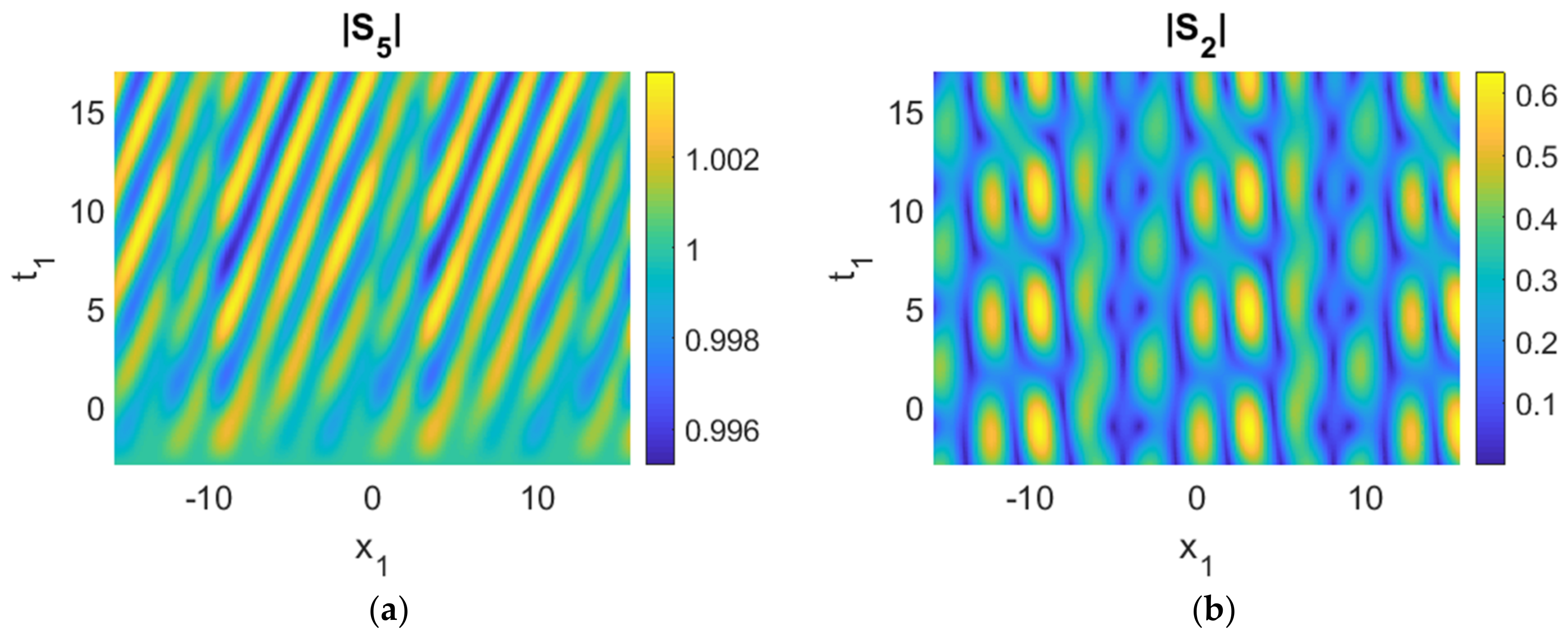
3.1. Components (3, 5, 1) being the Rogue Waves, and Modes 2 and 4 being the Plane Waves

We first study the case where one triad, e.g., (3, 5, 1) (Equation (6)), exhibits rogue modes, while members of the other triad, e.g., (4, 5, 2), i.e., mode 4 and mode 2, are in plane wave configurations (mode 5 is the common member of the two triads). The initial conditions for the coupled triads are then expressed analytically as

$$\begin{array}{l}{S}_1(x_1,t_1)=A_1(x_1,t_1), S_3(x_1,t_1)=A_2(x_1,t_1), S_5(x_1,t_1)=A_3(x_1,t_1),\\ S_2(x_1,t_1)=S_{2,p}(x_1,t_1), S_4(x_1,t_1)=S_{4,p}(x_1,t_1).\end{array}$$

(14)

Numerical simulations were performed according to standard split-step schemes (Figure 3). Comparisons of the maximum displacements of the wave profiles between the analytical approach and numerical results are displayed (

Table 1. Maxima of numerical and analytical results with a starting time of t_1,0 = −3. (Amplitude S_n as solutions of Equation (7)).

Components	Numerical Amplitude	Analytical Amplitude
S1	1.7730	2.8284
S3	2.2225	4
S5	1.6093	2.8284
S2	1.3844	1
S4	1.5193	1

).

The magnitude of the wave envelopes, |S_k| (k = 1, 2, 3, 4, 5) display periodic growth and decay cycles, which constitute the hallmark of FPUT. This is triggered by the rogue waves of the (3, 5, 1) triad (Figure 3a–e)). The evolution of mode 3 (|S₃|) is especially remarkable, as it combines both the features of FPUT and a rogue wave. To a certain extent, this pattern also appears in |S₁|. The periodic energy transfer among the various modes can be vividly observed (Figure 3a–e) and Table 1). Maxima of some |S_k| profiles correspond to minima of the other triad modes (Figure 3f). For this particular example, |S₃| and |S₅| are roughly in phase, with wave profiles increasing and decreasing at the same time. The other member of the (3, 5, 1) triad, |S₁|, is out of phase. The analytical reason comes from the signs of the interaction coefficients, namely, γ₁ < 0, γ₃ = γ_5a > 0. More precisely, when |S₃| and |S₅| reach the maximum (minimum), |S₁| attains the minimum (maximum), a clear demonstration of energy exchange for these triads. Furthermore, |S₂| and |S₄|, members of the other triad excited due to coupling, also exchange energy among themselves. Indeed energy transfer occurs among |S₁|, |S₃|, |S₅|, |S₂|, and |S₄|. This is especially clear for t₁ > 10 for the present choice of parameters. We observe that energy of |S₁| and |S₄| is transferred to |S₅| and |S₂|. This decrease in energy of |S₁| is again due to the sign of the interaction coefficient, γ₁ < 0.

To clarify the energy transfer mechanisms among modes of the (3, 5, 1) and (4, 5, 2) triads, control experiments were conducted with some interaction coefficients set to be zero:

• On setting the coefficients γ₂, γ₄ and γ_5b to be 0, energy only flows among members of the isolated triad (3, 5, 1). The other modes S₂ and S₄ just oscillate independently, as they are governed by the evolution equations

  $$\frac{\partial S_2}{\partial t_1}+c_{g2}\frac{\partial S_2}{\partial x_1}=0; \frac{\partial S_4}{\partial t_1}+c_{g4}\frac{\partial S_4}{\partial x_1}=0.$$

  (15)
  On examining Figure 3 and Figure 4, one can observe that energy transfer not only exists among |S₁|, |S₃|, |S₅| (|S₁| and |S₃| → |S₅|), but can also flow from triad (3, 5, 1) to triad (4, 5, 2) via the common member.
• On the other hand, one can also set the parameters γ₁, γ₃, and γ_5a to be zero (Figure 5), but maintain nonzero interaction coefficients in the other triad. Simulations can also be conducted. Qualitatively similar conclusions can be drawn, i.e., a rogue wave can trigger FPUT. Energy transfer also appears among |S₂|, |S₄|, |S₅| (|S₂| and |S₄| → |S₅|).

3.2. Components (3, 5, 1) as Plane Waves, Modes 2, 4 as Plane Waves with Perturbations

Next we consider the scenario where all modes start with a plane wave configuration. The initial conditions for the coupled triad are

$$\begin{array}{l}{S}_1(x_1,t_1)=S_{1,p}(x_1,t_1), S_3(x_1,t_1)=S_{3,p}(x_1,t_1), S_5(x_1,t_1)=S_{5,p}(x_1,t_1),\\ S_2(x_1,t_1)=S_{2,p}(x_1,t_1)+\mathsf{\delta }\cos (x), S_4(x_1,t_1)=S_{4,p}(x_1,t_1)+\mathsf{\delta }\cos (x).\end{array}$$

(16)

A small perturbation, measured by the parameter δ, is introduced to initiate the motion. Numerical simulations with split-step schemes are conducted (Figure 6). The maximum values of the wave profiles from the numerical and analytical approaches are displayed in

Table 2. Maxima of numerical and analytical rogue waves with time starting at t_1,0 = −3.

Components	Numerical Amplitude	Analytical Amplitude
S1	1.1060	1
S3	1.7826	1
S5	2.4633	1
S2	0.6634	0.1
S4	0.7256	0.1

.

Growth and decay cycles, i.e., FPUT, can still be triggered in |S_k| (k = 1, 2, 3, 4, 5) with the initial conditions of perturbed plane waves (Equation (15)). Phenomena similar to those of the previous section can still be observed (Figure 6), i.e., the variations of |S₃| and |S₅| are roughly in phase: increasing and decreasing at the same time, while |S₁| is out of phase with these two modes. More precisely, when |S₃| and |S₅| reach the maximum (minimum), |S₁| attains the minimum (maximum), as the signs of γ₁, γ₃, and γ_5a are the same as those in Figure 3. In addition, the fluctuations of the maximum amplitudes of |S₂| and |S₄| are very small. For a sufficiently small time (t₁ < 5 for parameters chosen here), energy transfer occurs between |S₂| and |S₄| only, arising from the small perturbations in the linear stage of modulation instability. For a larger time (t₁ > 5 in the present case), energy transfer occurs among |S₁|, |S₃|, |S₅|, |S₂|, and |S₄| in the nonlinear stage of modulation instability. Furthermore, we note these features:

(a)

if ρ₂, ρ₄ are small, exchange and oscillations of S₁, S₃, S₅ can be maintained;

(b)

if at least one of ρ₂ or ρ₄ is order one, then the oscillations exhibited by S₁, S₃, S₅ are distorted.

Comparing Figure 6f with Figure 3f, we conclude that:

• Energy transfer can arise immediately among |S₁|, |S₃|, and |S₅|, with the initial conditions being rogue wave modes (Figure 3f);
• Energy transfer occurs among |S₁|, |S₃|, |S₅|, |S₂|, and |S₄| in the nonlinear stage of modulation instability.

To highlight the energy exchange between the (3, 5, 1) and (4, 5, 2) triads, control experiments similar to previous sections (Figure 6) were performed for comparison (Figure 7 and Figure 8):

• We first consider the energy flow in an isolated triad (3, 5, 1) with γ₂ = γ₄ = 0 (Figure 7). The parameter γ_5b is critical for the movement of energy because |S₂| and |S₄| are perturbed by the noise. Comparing Figure 6 with Figure 7, the results show that the energy of perturbations flows to |S₁|, |S₃| and |S₅|. Furthermore, energy transfer occurs among |S₁|, |S₃|, |S₅| (|S₁| → |S₃| and |S₅|), as well as triads (3, 5, 1) and (4, 5, 2) ((4, 5, 2) → (3, 5, 1)), simultaneously.
• Setting γ₁ = γ₃ = γ_5a = 0 and comparing Figure 6 with Figure 8, energy exchange can be observed between |S₂| and |S₄|. The energy transfer among |S₂|, |S₄|, |S₅| is insignificant due to the small magnitude of the parameter γ_5b. However, energy movement among |S₂|, |S₄|, |S₅| (|S₂| and |S₄| to |S₅|) will still take place if the simulation is continued for a sufficiently long time.

4. Simulations with Other Choices of Input Parameters

Theoretically, five out of the six interaction coefficients of the coupled triad system (Equation (7)) can in principle be normalized to unity. For convenience, we shall nominally take γ_5b as a free parameter. In the previous section, we took all the other ‘γ’ as small integers (±1) or fractions (±1/2). In practice, these interactions are calculated from density profilesand velocity eigenfunctions of stratified fluids (Appendix A). Hence it would be instructive to perform computer simulations with realistic or fluid mechanics-inspired values of ‘γ’. First, we note that signs of the interaction coefficients generally proceed such as:

$${\mathsf{\gamma }}_1>0, {\mathsf{\gamma }}_3<0, {\mathsf{\gamma }}_{5a}>0; {\mathsf{\gamma }}_2<0, {\mathsf{\gamma }}_4>0, {\mathsf{\gamma }}_{5b}<0.$$

(17)

4.1. Components (3, 5, 1) Being Rogue Waves, Modes 2 and 4 Being Plane Waves

The initial conditions for the coupled triad are chosen as

$$\begin{array}{l}{S}_1(x_1,t_1)=A_1(x_1,t_1), S_3(x_1,t_1)=A_2(x_1,t_1), S_5(x_1,t_1)=A_3(x_1,t_1),\\ S_2(x_1,t_1)=S_{2,p}(x_1,t_1), S_4(x_1,t_1)=S_{4,p}(x_1,t_1).\end{array}$$

(18)

The properties established in the previous section remain valid. More precisely, |S₁|, |S₃|, and |S₅| exhibit a mixture of FPUT growth/decay cycles and rogue wave type outburst (Figure 9). With c_g1 < 0, c_g3 > 0 and c_g5 > 0, the wave profiles of |S₃| and |S₅| are going forward, while |S₁| travels backward. Movement of energy can be traced by the locations of maxima of |S_k| (Figure 9). With γ₁ = γ_5a > 0, γ₃ < 0, the wave profiles of |S₁| and |S₅| are in phase, while |S₃| is 180 degrees out of phase with these two.

4.2. Components (3, 5, 1) as Plane Waves, Modes 2, 4 Being Plane Waves with Perturbations

The initial conditions are selected to be

$$\begin{array}{l}{S}_1(x_1,t_1)=S_{1,p}(x_1,t_1), S_3(x_1,t_1)=S_{3,p}(x_1,t_1), S_5(x_1,t_1)=S_{5,p}(x_1,t_1),\\ S_2(x_1,t_1)=S_{2,p}(x_1,t_1)+\mathsf{\delta }\cos (x), S_4(x_1,t_1)=S_{4,p}(x_1,t_1)+\mathsf{\delta }\cos (x).\end{array}$$

(19)

All components |S_k| (k = 1, 2, 3, 4, 5) display FPUT growth and decay cycles (Figure 10a–e). The propagation directions of |S₂| and |S₄| are different owing to the different signs of the group velocities, c_g2 < 0, c_g4 > 0. Energy exchange can be tracked by the locations of maxima of |S_k| (Figure 10f). Wave profiles |S₁| and |S₅| are roughly in phase: increasing and decreasing at the same time, while |S₃| is out of phase, a manifestation of the signs of the interaction coefficients, γ₁ = γ_5a > 0, γ₃ < 0. Simultaneously, energy transfer also exists among |S₂|, |S₄|, and |S₅|. For a reasonably small time (t₁ < 5 here), energy only moves between |S₂| and |S₄|, resulting from the small perturbations in the linear stage of modulation instability. For a larger time (t₁ > 5), the energy flows among |S₁|, |S₃|, |S₅|, |S₂|, and |S₄| in the nonlinear stage of modulation instability.

5. Discussions and Conclusions

A remark on the applications of the present formulation to physical oceanography is appropriate. The nonlinear Schrödinger equation and the Peregrine breather are widely used models for describing the dynamics of surface wave packets and surface rogue waves. One scientifically documented rogue wave was the Draupner Wave of 1 January 1995. If we compute the coefficients of the Schrödinger equation with the water depth conditions at the location of the Draupner Wave, the coefficients are generally of order unity, and hence no scaling is necessary. Since the Peregrine breather has a maximum displacement of three times the background plane wave, a background wave train of 8 m will produce a rogue wave with an amplitude of roughly 25 m, which is consistent with observations.

For internal rogue waves described by the triad equations, the interaction coefficients may differ drastically from unity, and thus rescaling would be necessary. As an illustrative example, we can consider an average ocean depth of say 4000 m. The corresponding interaction coefficients can be obtained from Figure 2 by choosing a non-dimensional water depth of H = 4, if we choose a reference length scale of 1 km. The numerical values of the coefficients are γ₁ = 7.9946 × 10⁻⁴, γ₂ = −5.4641 × 10⁻⁴, γ₃ = −0.0562, γ₄ = 0.1823, γ_5a = 0.0244, γ_5b = −0.1143.

To estimate the actual amplitude in a realistic oceanic condition, we employ the formulation

S₁ = A₁/(|γ₃||γ_5a|)^1/2, S₃ = A₂ /(|γ₁||γ_5a|)^1/2, S₅ = A₃ /(|γ₁||γ₃|)^1/2,

(20)

where S_n and A_n are amplitudes in Equations (7) and (11), respectively. As the exact solutions of Equation (12) exhibit an amplitude of roughly two, the actual maximum displacements will be of the order of 50 to 200 m in the interior of the oceans. The spatial size of such internal rogue waves will scale with the wavelength of the packet. The temporal duration will again follow the ‘non-dimensionalization’ time unit, i.e., the square root of (length scale/gravity). If the length scale is 1 km and gravity is taken as 10 m s⁻², the time scale is in multiples of 10 s. The typical rogue wave solution of Equation (11) takes about six time units to go through a growth–decay cycle, and hence this corresponds to 1 min in real time. For internal waves with a length scale much larger than 1 km, the spatial extent and time period will be correspondingly larger.

A widely adopted model in a deterministic (as opposed to probabilistic) approach to water waves is the nonlinear Schrödinger equation (NLS), where the salient features are the Peregrine breather and modulation instability. Two features associated with NLS have generated discussion and debate in the literature, namely, time scale and quadratic versus cubic nonlinearity. For NLS, the asymptotic time scale of evolution is ε²t, where ε is a non-dimensional, small amplitude parameter. For triad resonance, the time scale is εt, and is thus much faster. One drawback of the analytical formulation of breathers and rogue waves of NLS is the assumption of a long crested wave, which might make realization in terms of field observation difficult. A competing theory, utilizing interference of second order waves, has been suggested in the literature [29]. Hence systems with quadratic nonlinearities deserve a penetrating study, and we believe that the triad resonance equations constitute an appropriate candidate.

Coupled triads with one common member can exist in stratified fluids with constant buoyancy frequency, and are important in the general context of mathematical physics [30,31]. The evolution equations for weakly nonlinear, slowly varying, narrow banded wave packets are then derived by perturbation theory. We focused on the case where the common member is a daughter wave (passive mode). This is in sharp contrast with our previous work [7], where the common member was the parent wave (active mode). Moreover, rogue modes, instead of plane waves, were used as initial conditions. While our earlier work included time dependence only [7], spatial dependence is incorporated here. Generally the signs of the interaction coefficients are critical for the energy transfer process. If the interaction coefficients of two components in a triad have the same sign, the evolution of the corresponding amplitudes tends to be in phase. With the common member being the daughter wave (passive modes), the sign patterns of the interaction coefficients are not affected drastically in comparison with our previous work on a common parent wave (active mode). However, the magnitudes are modified. From numerical simulations, if the common member is the parent wave (active mode), energy can be readily transferred from one triad to the two daughter waves (passive modes) in the other triad through the common parent member [7]. However, if the common member is a daughter wave (passive mode), this catalyst mechanism of moving energy appears to be much less efficient. The underlying reason for this is not properly understood. Whether the structure of evolution equations plays a role will constitute a topic of future research. Hence triad resonance might provide a feasible mechanism of energy transfer among modes in addition to other theories in the literature such as weak turbulence [32,33].

In addition to their relevance in a theoretical context, the numerical simulations performed here will enhance physical insights into extreme waves in the oceans. Although rogue waves for an isolated triad have been derived in a mathematical physics setting in the past ten years, here we apply these formulations to oceanic internal waves. More precisely, we demonstrated the existence of FPUT type growth and decay cycles for the triad equations. Furthermore, we studied a system of coupled triads, where analytical solutions are not available. Nevertheless, the nonlinear dynamical interplay between rogue modes and plane waves is intriguing and was demonstrated through computational studies. Through these simulations, the computational evidence shows that the FPUT and immediate energy transfer can be triggered by rogue waves. Moreover, the linear and nonlinear stages of modulation instability are related to the transfer of energy among the five waves. Finally, the evolution of wave profiles and energy transfer depends crucially on the initial conditions and the sign patterns of the interaction coefficients.

While our attention mostly focused on the theoretical aspects, remarks on practical applications to physical oceanography are in order. One contrast with long wave models of internal rogue modes [17] is relevant. Assuming an ocean depth of 1000 m, the wavelength for a Korteweg-de Vries model to be valid must be at an order of magnitude of 10,000 m or longer. In contrast, the fast oscillations of the wave packets involved in triad resonance do not need to conform to a long wave scaling and can be comparable to just the water depth. Indeed there are recorded oceanic data in the literature on trains or packets of internal wave oscillations within one or a few kilometers [34,35].

There remain many formidable challenges in terms of future research opportunities. One direction is to relax the assumption of a constant buoyancy frequency (or the squared value as N²). Indeed taking N² as the square of the hyperbolic secant will have both theoretical and physical significance. Theoretically, the eigenfunctions can be obtained in closed forms using hyperbolic functions. Physically, a sharply peaked profile of N² is a realistic approximation of the oceans, as the density can experience a sharp change across a pycnocline. Another limiting case of sharp density change is modeled by a two-layer fluid, which has been employed by fluid dynamicists for over a century. Promising results are awaiting our further efforts.

References

1. Phillips, O.M. On the dynamics of unsteady gravity waves of finite amplitude Part 1. The elementary interactions. J. Fluid Mech. 1960, 9, 193–217. [Google Scholar] [CrossRef]
2. Phillips, O.M. On the dynamics of unsteady gravity waves of finite amplitude Part 2. Local properties of a random wave field. J. Fluid Mech. 1961, 11, 143–155. [Google Scholar] [CrossRef]
3. McGoldrick, L.F. Resonant interactions among capillary-gravity waves. J. Fluid Mech. 1965, 21, 305–331. [Google Scholar] [CrossRef]
4. Ball, F.K. Energy transfer between external and internal gravity waves. J. Fluid Mech. 1964, 19, 465–478. [Google Scholar] [CrossRef]
5. Thorpe, S.A. On wave interactions in a stratified fluid. J. Fluid Mech. 1966, 24, 737–751. [Google Scholar] [CrossRef]
6. Biswas, L.; Shukla, P. Stability analysis of a resonant triad in a stratified uniform shear flow. Phys. Rev. Fluids 2021, 6, 014802. [Google Scholar] [CrossRef]
7. Pan, Q.; Peng, N.N.; Chan, H.N.; Chow, K.W. Coupled triads in the dynamics of internal waves: Case study using a linearly stratified fluid. Phys. Rev. Fluids 2021, 6, 024802. [Google Scholar] [CrossRef]
8. Dauxois, T.; Joubaud, S.; Odier, P.; Venaille, A. Instabilities of internal gravity wave beams. Annu. Rev. Fluid Mech. 2018, 50, 131–156. [Google Scholar] [CrossRef] [Green Version]
9. Sutherland, B.R.; Jefferson, R. Triad resonant instability of horizontally periodic internal modes. Phys. Rev. Fluids 2020, 5, 034801. [Google Scholar] [CrossRef]
10. Karimi, H.H.; Akylas, T.R. Near-inertial parametric subharmonic instability of internal wave beams. Phys. Rev. Fluids 2017, 2, 074801. [Google Scholar] [CrossRef]
11. Varma, D.; Mathur, M. Internal wave resonant triads in finite-depth non-uniform stratifications. J. Fluid Mech. 2017, 824, 286–311. [Google Scholar] [CrossRef]
12. Fan, B.; Akylas, T.R. Effect of background mean flow on PSI of internal wave beams. J. Fluid Mech. 2019, 869, R1. [Google Scholar] [CrossRef]
13. Obuse, K.; Yamada, M. Three-wave resonant interactions and zonal flows in two-dimensional Rossby-Haurwitz wave turbulence on a rotating sphere. Phys. Rev. Fluids 2019, 4, 024601. [Google Scholar] [CrossRef] [Green Version]
14. Bustamante, M.D.; Kartashova, E. Effect of the dynamical phases on the nonlinear amplitudes’ evolution. Europhys. Lett. 2009, 85, 34002. [Google Scholar] [CrossRef] [Green Version]
15. Dysthe, K.; Krogstad, H.E.; Muller, P. Oceanic rogue waves. Annu. Rev. Fluid Mech. 2008, 40, 287–310. [Google Scholar] [CrossRef]
16. Onorato, M.; Residori, S.; Bortolozzo, U.; Montina, A.; Arecchi, F. Rogue waves and their generating mechanisms in different physical contexts. Phys. Rep. 2013, 528, 47–89. [Google Scholar] [CrossRef]
17. Grimshaw, R.; Pelinovsky, E.; Taipova, T.; Sergeeva, A. Rogue internal waves in the ocean: Long wave model. Eur. Phys. J. Spec. Top. 2010, 185, 195–208. [Google Scholar] [CrossRef]
18. Talipova, T.; Kurkina, O.; Kurkin, A.; Didenkulova, E.; Pelinovsky, E. Internal wave breathers in the slightly stratified fluid. Microgravity Sci. Technol. 2020, 32, 69–77. [Google Scholar] [CrossRef]
19. Bokaeeyan, M.; Ankiewicz, A.; Akhmediev, N. Bright and dark rogue internal waves: The Gardner equation approach. Phys. Rev. E 2019, 99, 062224. [Google Scholar] [CrossRef]
20. Baronio, F.; Conforti, M.; Degasperis, A.; Lombardo, S. Rogue waves emerging from the resonant interaction of three waves. Phys. Rev. Lett. 2013, 111, 114101. [Google Scholar] [CrossRef] [Green Version]
21. Coppini, F.; Santini, P.M. Fermi-Pasta-Ulam-Tsingou recurrence of periodic anomalous waves in the complex Ginzburg-Landau and in the Lugiato-Lefever equations. Phys. Rev. E 2020, 102, 062207. [Google Scholar] [CrossRef]
22. Gallavotti, G. The Fermi-Pasta-Ulam Problem: A Status Report, 1st ed.; Springer: Berlin/Heidelberg, Germany, 2008. [Google Scholar]
23. Yuen, H.C., Jr.; Ferguson, W.E.F. Relationship between Benjamin–Feir instability and recurrence in the nonlinear Schrödinger equation. Phys. Fluids 1978, 21, 1275–1278. [Google Scholar] [CrossRef]
24. Hasselman, K. A criterion for nonlinear wave stability. J. Fluid Mech. 1967, 30, 737–739. [Google Scholar] [CrossRef]
25. Kartashova, E.; L’vov, V.S. Cluster dynamics of planetary waves. Europhys. Lett. 2008, 83, 50012. [Google Scholar] [CrossRef] [Green Version]
26. Yoshinaga, T.; Wakamiya, M.; Kakutani, T. Recurrence and chaotic behavior resulting from nonlinear interaction between long and short waves. Phys. Fluids A 1991, 3, 83. [Google Scholar] [CrossRef]
27. Wabnitz, S.; Akhmediev, N. Efficient modulation frequency doubling by induced modulation instability. Opt. Commun. 2010, 283, 1152–1154. [Google Scholar] [CrossRef]
28. Vanderhaegen, G.; Szriftgiser, P.; Kudlinski, A.; Conforti, M.; Trillo, S.; Droques, M.; Mussot, A. Observation of four Fermi-Pasta-Ulam-Tsingou recurrences in an ultra-low-loss optical fiber. Opt. Express 2020, 28, 17773–17781. [Google Scholar] [CrossRef] [PubMed]
29. Fedele, F.; Brennan, J.; Ponce de León, S.; Dudley, J.; Dias, F. Real world ocean rogue waves explained without the modulational instability. Sci. Rep. 2016, 6, 27715. [Google Scholar] [CrossRef] [PubMed]
30. Kartashova, E.; Shugan, I.V. Dynamical cascade generation as a basic mechanism of Benjamin-Feir instability. Europhys. Lett. 2011, 95, 30003. [Google Scholar] [CrossRef]
31. Kartashova, E. Nonlinear Resonance Analysis: Theory, Computation, Applications; Cambridge University Press: Cambridge, UK, 2010. [Google Scholar]
32. Pelinovskiy, E.N.; Raevsky, M.A. Weak turbulence of internal waves in the ocean. Izv. Atmos. Ocean. Phys. 1977, 13, 130–134. [Google Scholar]
33. Kharif, C.; Pelinovsky, E.; Slunyaev, A. Rogue Waves in the Ocean, 1st ed.; Springer: Berlin/Heidelberg, Germany, 2009. [Google Scholar]
34. Orr, M.H.; Mignerey, P.C. Nonlinear internal waves in the South China Sea: Observation of the conversion of depression internal waves to elevation internal waves. J. Geophys. Res. Ocean. 2003, 108. [Google Scholar] [CrossRef]
35. Kaminski, A.K.; Flynn, M.R. Modal decomposition of polychromatic internal wave fields in arbitrary stratifications. Wave Motion 2020, 95, 102549. [Google Scholar] [CrossRef]
Figure 1. Schematic diagram of coupled triads with all five participating waves traveling in the same direction. A solid dot on the m = 5 branch represents the common member, with modes 1, 3, and 5 forming one triad and modes 2, 4, and 5 the other triad. As an illustrative example, the numerical values of the corresponding wave numbers and wave frequencies are: (k1 = 0.5153, ω1 = 0.1619), (k2 = 0.5160, ω2 = 0.0819), (k3 = 3.5153, ω3 = 0.3495), (k4 = 3.5160, ω4 = 0.2694), (k5 = 3, ω5 = 0.1876).
Jmse 09 00577 g001
Figure 2. Variation of the interaction coefficients with the channel depth H.
Jmse 09 00577 g002
Figure 3. (ae) Evolution of the five wave components; (f) time history of the moduli of the envelopes, |Sk|. Parameters used were cg1 = 2, cg3 = 1, cg5 = 0.5, cg2 = 0.1, cg4 = 0.1, γ1 = −0.1, γ3 = 0.1, γ5a = 0.1, γ2 = −0.1, γ4 = 0.1, γ5b = −0.01, r1 = 1, r2 = 1, r3 = 0, q = 1, a2 = 1, ρ1 = ρ2 = ρ3 = ρ4 = ρ5 = 1.
Jmse 09 00577 g003aJmse 09 00577 g003b
Figure 4. (ae) Control experiment (only |S1|, |S3| and |S5| oscillate, |S2|, |S4| mostly unchanged); (f) time history of the moduli of the envelopes, |Sk|. Parameters used were cg1 = 2, cg3 = 1, cg5 = 0.5, cg2 = 0.1, cg4 = 0.1, γ1 = −0.1, γ3 = 0.1, γ5a = 0.1, γ2 = 0, γ4 = 0, γ5b = 0, r1 = 1, r2 = 1, r3 = 0, q = 1, a2 = 1, ρ1 = ρ2 = ρ3 = ρ4 = ρ5 = 1.
Jmse 09 00577 g004aJmse 09 00577 g004b
Figure 5. (ae) Control experiment (only |S2|, |S4| and |S5| oscillate, |S1|, |S3| move as plane wave); (f) time history of the moduli of the envelopes, |Sk|. Parameters used were cg1 = 2, cg3 = 1, cg5 = 0.5, cg2 = cg4 = 0.1, γ1 = γ3 = γ5a = 0, γ2 = −0.1, γ4 = 0.1, γ5b = −0.01, r1 = 1, r2 = 1, r3 = 0, q = 1, a2 = 1, ρ1 = ρ2 = ρ3 = ρ4 = ρ5 = 1.
Jmse 09 00577 g005aJmse 09 00577 g005b
Figure 6. (ae) The evolution of five wave components; (f) time history of the moduli of the envelopes, |Sk|. Parameters used were cg1 = 2, cg3 = 1, cg5 = 0.5, cg2 = −0.1, cg4 = 0.1, γ1 = 1, γ3 = −1, γ5a = −1, γ2 = −0.5, γ4 = 0.5, γ5b = −0.01, a2 = 1, ρ1 = ρ3 = ρ5 = 1, ρ2 = ρ4 = 0.1, δ = 0.4.
Jmse 09 00577 g006aJmse 09 00577 g006b
Figure 7. (ae) Control experiment (only |S1|, |S3| and |S5| oscillate, |S2|, |S4| move as plane wave); (f) time history of the moduli of the envelopes, |Sk|. Parameters used were cg1 = 2, cg3 = 1, cg5 = 0.5, cg2 = −0.1, cg4 = 0.1, γ1 = 1, γ3 = γ5a = −1, γ2 = γ4 = 0, γ5b = −0.01, a2 = 1, ρ1 = ρ3 = ρ5 = 1, ρ2 = ρ4 = 0.1, δ = 0.4.
Jmse 09 00577 g007aJmse 09 00577 g007b
Figure 8. (ac) Control experiment (only |S2|, |S4| and |S5| oscillate, |S1|, |S3| mostly unchanged); (d) time history of the moduli of the envelopes, |Sk|. Parameters used were cg1 = 2, cg3 = 1, cg5 = 0.5, cg2 = −0.1, cg4 = 0.1, γ1 = γ3 = γ5a = 0, γ2 = −0.5, γ4 = 0.5, γ5b = −0.01, a2 = 1, ρ1 = ρ3 = ρ5 = 1, ρ2 = ρ4 = 0.1, δ = 0.4.
Jmse 09 00577 g008aJmse 09 00577 g008b
Figure 9. (ac) Evolution of the wave components; (d) time history of the moduli of the envelopes, |Sk|. Parameters used were cg1 = −0.5, cg3 = 1, cg5 = 0.5, cg2 = −0.1, cg4 = 0.6, γ1 = 0.1, γ3 = −0.1, γ5a = 0.1, γ2 = −0.1, γ4 = 0.1, γ5b = −0.01, r1 = 1, r2 = 1, r3 = 0, q = 1, a2 = 1, ρ1 = ρ2 = ρ3 = ρ4 = ρ5 = 1.
Jmse 09 00577 g009
Figure 10. (ae) Evolution of the five wave components; (f) time history of the moduli of the envelopes, |Sk|. Parameters used were cg1 = −0.5, cg3 = 1, cg5 = 0.5, cg2 = −0.1, cg4 = 0.6, γ1 = 1, γ3 = −1, γ5a = 1, γ2 = −0.5, γ4 = 0.5, γ5b = −0.05, a2 = 1, ρ1 = ρ3 = ρ5 = 1, ρ2 = ρ4 = 0.1, δ = 0.4.
Jmse 09 00577 g010