Spatial Variability and Trends of Marine Heat Waves in the Eastern Mediterranean Sea over 39 Years

Abstract

Marine heatwaves (MHWs) can cause devastating impacts on marine life. The frequency of MHWs, gauged with respect to historical temperatures, is expected to rise significantly as the climate continues to warm. The MHWs intensity and count are pronounced with many parts of the oceans and semi enclosed seas, such as Eastern Mediterranean Sea (EMED). This paper investigates the descriptive spatial variability and trends of MHW events and their main characteristics of the EMED from 1982 to 2020 using Sea Surface Temperature (SST) data obtained from the National Oceanic and Atmospheric Administration Optimum Interpolation ([NOAA] OI SST V2.1). Over the last two decades, we find that the mean MHW frequency and duration increased by 40% and 15%, respectively. In the last decade, the shortest significant MHW mean duration is 10 days, found in the southern Aegean Sea, while it exceeds 27 days off the Israeli coast. The results demonstrate that the MHW frequency trend increased by 1.2 events per decade between 1982 and 2020, while the MHW cumulative intensity (i_cum) trend increased by 5.4 °C days per decade. During the study period, we discovered that the maximum significant MHW SST event was 6.35 °C above the 90th SST climatology threshold, lasted 7 days, and occurred in the year 2020. It was linked to a decrease in wind stress, an increase in air temperature, and an increase in mean sea level pressure.

1. Introduction

In many parts of the world, heatwaves are growing increasingly common and prevalent. It creates significant climatic extremes in oceanic and atmospheric systems, which can have catastrophic ecological impacts and huge socioeconomic effects [1,2,3]. The study of Marine Heat Waves is important for understanding and predicting climate change and its impact on ocean ecosystems. Marine heat wave (MHW), according to [4], is ‘’a prolonged discrete anomalously warm water event that can be described by its duration, intensity, rate of evolution, and spatial coverage’’. It was suggested that a linear classification scheme be used by [5], where MHWs are defined based on temperature exceedance from local climatology, which will impact the classification. The probability of the occurrence of MHWs is impacted by SST climatological values as described in [2,6,7,8]. Changes and variability in SST climatological values, as described in [7,8], will have an impact on the definition and probability of occurrence of MHW. These extreme events lead to a widespread mortality of benthic invertebrates [9] and loss of seagrass meadows [10]. Over the last four decades, the international oceanographic community, regulators and policy makers have paid close attention to the EMED, namely because in this region variations in processes of relevance for the global climate change take place over relatively short space and time scale [11,12,13].

In the summer of 2003, one of the first-detected MHWs occurred in the Mediterranean which lasted over a month due to an increase of air temperature, a reduction of wind stress, and air-sea exchanges [14,15,16]. That phenomenon led to an anomalous SST warming in the EMED area during the heatwave of 2003, on the order of +5 °C above climatology [17].

Reference [18] investigated the future evolution (1976–2100) of SST and marine heatwaves in the Mediterranean Sea using a local, climatological 99th percentile threshold based on historical-climate daily SST (1976–2005). The dataset 1982–2012 revealed an annual frequency of 0.8 events per year, with MHWs lasting for a maximum of 1.5 months between July and September, while covering a maximum of 90% of the Mediterranean Sea surface. The longest and most severe event of that period corresponded to the MHW of 2003, with the highest mean intensity and maximum event coverage. The authors have concluded that the MHWs will become stronger and more intense in response to increasing greenhouse gas forcing, particular near the end of the century.

Unfortunately, very few studies on the MHW have been published in the EMED, and the topic is still being debated, as mentioned by [19].

In this study 39 years (1982–2020) of SST data have been analyzed to demonstrate the SST trend and interannual variability based on Empirical Orthogonal Function (EOF). This paper describes the main characteristics of MHWs in the EMED. The authors detect and analyze the most intense MHW events observed in the EMED during the study period, as well as their relationship to atmospheric conditions.

2. Data and Methods of Analysis

The Eastern Mediterranean (EMED) region includes the Ionian and the Levantine basins with two other marginal seas; the Adriatic and the Aegean as shown in Figure 1a. The EMED reaches a depth of over 3000 m off Mersa Matruh at the western part of Egypt and 4000 m to the southeast of Rhodes [20,21] see Figure 1b. The mean depth of the EMED basin is about 2000 m. The shelf is usually extending for no more than 8 km, except off the Nile Delta, where the 200 m contour is traced at 60 km offshore, in the Sicily Strait and the Adriatic Sea. The most important islands in the EMED are Sicily, Malta, Crete, Rhodes, and Cyprus. The study area extending from 30° to 42° N and from 13° to 36.5° E is shown in Figure 1a,b. This area is covering most of the EMED. In this section the authors will describe the data and methods of analysis used to obtain the results.

2.1. Sea Surface Temperature Data

The daily SST data used were obtained from the National Oceanic and Atmospheric Administration Optimum Interpolation Sea Surface Temperature from 1 January 1982 to 31 December 2020 ([NOAA] OI SST V2.1; [22]). The data are freely available on the NOAA website https://www.ncei.noaa.gov/data/sea-surface-temperature-optimum-interpolation/v2.1/access/avhrr/ (accessed on 10 January 2021). This data set is an interpolation of remotely sensed SSTs from the Advanced Very High Resolution Radiometer (AVHRR) imager into a regular grid of 0.25° and daily temporal resolution. AVHRR OI data for the EMED Sea were extracted from the global data, providing a 2624-point regularly gridded dataset spanning 14,245 days from 1 January 1982 to 31 December 2020.

2.2. Trend and Interannual Variabilty of SST

To demonstrate the spatiotemporal variability in SST over the EMED Sea, an EOF is calculated using the singular value decomposition (SVD) approach [23]. EOF analysis extracts the main mode of SST variability, providing us with a spatial pattern and a time-varying index known as the principal component (PC). The EOF analysis was applied to gridded monthly SST anomalies from 1982 to 2020. As described in [24], the SST anomalies were calculated by subtracting the historical climatological mean value at each grid point from the SST values at the same location (grid). Here, we are interested in interannual and longer time scales variability. So, prior to EOF decomposition, the seasonal cycle and linear trends were removed from the monthly means of SST anomalies at each grid point, and then the SST were normalized by dividing each point time series by its standard deviation. The mean seasonal cycle was estimated by calculating the mean monthly values for each calendar month at each grid point from 1982 to 2020. To obtain de-seasoned monthly values, the mean value of each month was subtracted from all corresponding months in all years. Linear trends of de-seasoned monthly SST anomaly are estimated by using the least squares method [25]. To assess the statistical significance of these trends, the original two-tailed modified Mann–Kendall test at 95% confidence interval was used [26,27]. The authors used a thirteen-month running mean to remove the higher frequency variability in order to highlight the interannual variability, as described in [28]. Refs. [29,30] provide examples of similar data filtration methods.

It is crucial for our study to determine the warmest period from the whole climatological SST time series, NOAA OI SST V2.1. To reach our goal we divided the SST time series into four periods, (P₁, 1 January 1982–31 December 1990), (P₂, 1 January 1991–31 December 2000), (P₃, 1 January 2001–31 December 2010) and (P₄, 1 January 2011–31 December 2020). The chosen of the first period P₁ is based on satellite NOAA OI SST V2.1 data availability. Then daily climatology was calculated from the P₁, P₂, P₃ and P₄ years employed in the analysis and smoothed with a monthly centred-moving mean.

2.3. Marine Heat Waves (MHWs) Calculations

The authors used [5] MHWs, definition, as a discrete prolonged anomalously warm-water events in a location, using the same daily SST database for the 1982–2020 period. The MATLAB toolbox [31] has been used to identify periods of time where temperatures were above the 90th percentile threshold relative to the climatology, and for a duration of at least 5 days. The authors identified the start and end dates and calculated the duration and intensity for each MHW event according to [5]. The climatological mean has been calculated from the daily Sea Surface Temperature (SST) data from 1 January 1982 to 31 December 2020 ([NOAA] OI SST V2.1; [22] following the [5] formula,

$${\mathrm{T}}_{\mathrm{m}}(\mathrm{j})={{\displaystyle \sum }}_{y={\mathrm{y}}_{\mathrm{s}}}^{{\mathrm{y}}_{\mathrm{e}}} {{\displaystyle \sum }}_{d=j-5}^{j+5}\frac{T \left(y,d\right)}{11 \left({\mathrm{y}}_{\mathrm{e}}-{\mathrm{y}}_{\mathrm{s}}+1\right)}$$

(1)

where, T_m is the climatological SST mean in °C calculated over a period from 1 January 1982 to 31 December 2020, to which all values are relative, j is the day of year, y_s and y_e are the start and end of the climatological base period respectively, and T is the daily SST on day d of year y. Then the 90th percentile threshold based on SST climatology period, T₉₀ (j) in °C are calculated according to [5] based on climatological SST mean (X) in °C over a period from 1 January 1982 to 31 December 2020 as follow:

T₉₀ (j) = P₉₀ (X)

(2)

According to [5] definition, MHWs occur when SSTs exceed the threshold, defined as the 90th percentile of SST variations (T₉₀ (j)) based on a 39-year climatological period (1982–2020), for at least five consecutive days. At each location and for each MHW, we calculated the event duration (time between start and end dates) and mean cumulative intensity. Associated annual statistics were then calculated, including the frequency of events (i.e., the number of discrete events occurring in each year),

t_e − t_s ≥ 5

(3)

where t_e, t_s: dates on which a MHW begins and ends. And D is the MHW Duration in Days that temperature exceeds the threshold, D = t_e − t_s.

Where P₉₀ is the 90th percentile and

X = {T(y,d)|y_s <= y <= y_e, j − 5 <= d <= j + 5}

(4)

Then, the MHWs main characteristics are (i_max) in °C, mean intensity (i_mean) in °C and (i_cum) in (°C Days):

i_max = max (T(t) − T_m (j))

(5)

$$\begin{gathered} {\mathrm{i}}_{\mathrm{mean}}=\overline{T\left(t\right)-\mathrm{Tm}\left(j\right)} \\ \mathbf{During}\mathbf{the}\mathbf{MHW}\mathbf{event} \\ {\mathrm{t}}_{\mathrm{s}}\le \mathrm{j}\le {\mathrm{t}}_{\mathrm{e}}\mathbf{and}\mathrm{j}\left({\mathrm{t}}_{\mathrm{s}}\right)\le \mathrm{j}\le \mathrm{j}\left({\mathrm{t}}_{\mathrm{e}}\right) \end{gathered}$$

(6)

$${\mathrm{i}}_{\mathrm{cum}}={{\displaystyle \int }}_{{\mathrm{t}}_{\mathrm{s}}}^{{\mathrm{t}}_{\mathrm{e}-1}}\left(T\left(\text{t}\right)-{\mathrm{T}}_{\mathrm{m}}\left(\mathrm{j}\right)\right)dt$$

(7)

i_cum: sum of daily intensity anomalies.

According to [5] during the MHW event:

T(t) > T₉₀ (j), t_s is the time, t,

while during time (t − 1) presents no MHW event

T(t − 1) < T₉₀ (j), t_e is the time, t, where t_e > t_s

T(t) < T₉₀ (j)

2.4. Atmospheric Variables Data

Atmospheric variables were obtained from the European Centre for Medium-Range Weather Forecasts (ECMWF) ERA5 [32]. Winds at 10 m elevation (U₁₀ and V₁₀), air temperature at 2 m elevation, and pressure at mean sea level were used. The dataset has 0.25° spatial resolution with hourly temporal step. Daily means were computed by averaging hourly data, and a daily climatology was built in the same manner as for SST, using the same period from 1982 to 2020. The wind stress components in east and north directions (τ_wx, τ_wy) were calculated according to [33] in (N/m²),

τ = C_D ρ_a |W| ∗ W

(8)

where ρ_a = 1.2 (kg/m³) is the density of air, C_D is the drag coefficient in Equation (8) is computed according to [34] while (W) is the wind speed component (m/s). The authors have computed the wind stress components to track 14–20 May 2020 MHW events which have the maximum intensity over the whole study period (1982–2020).

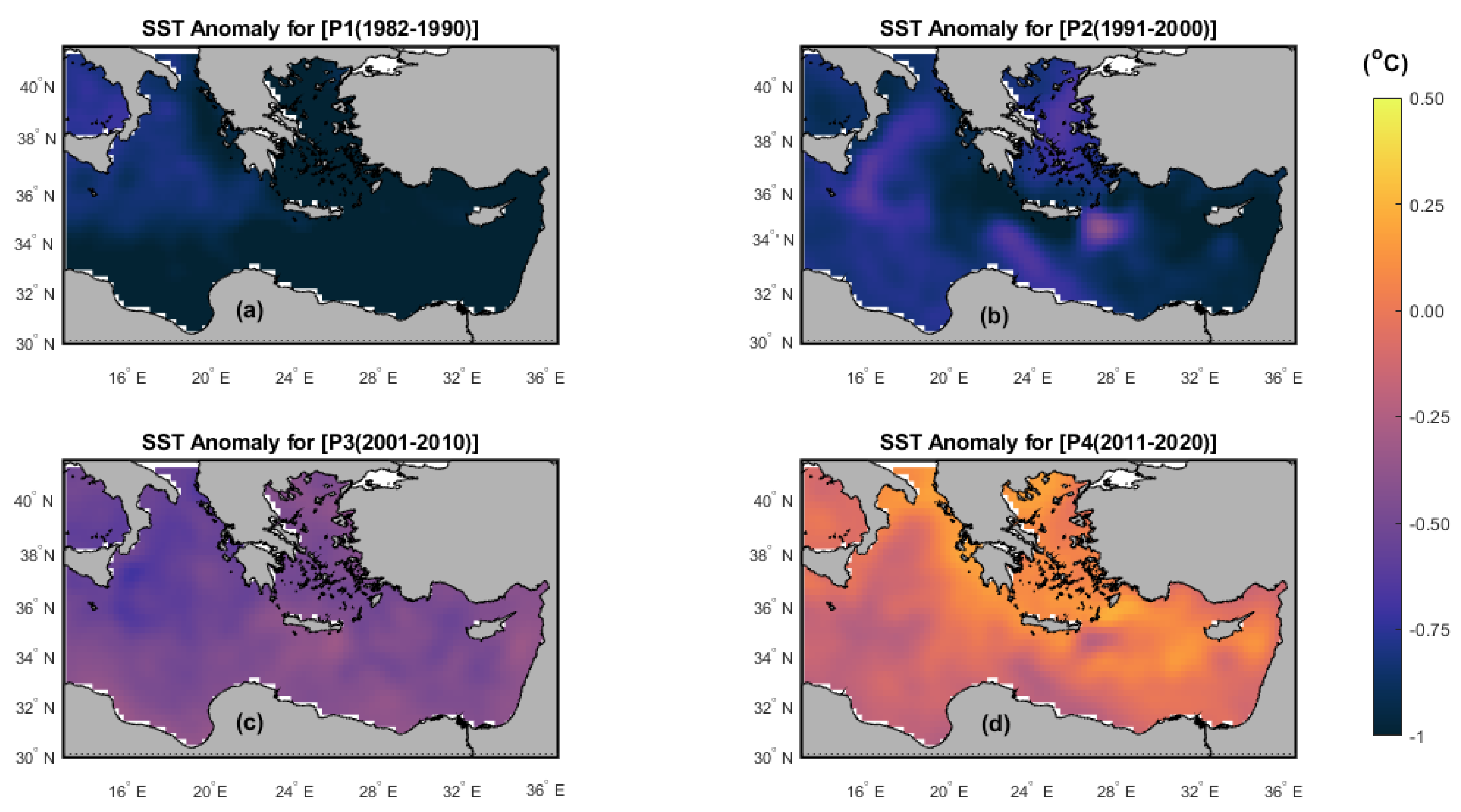
3. Description of the SST Data (1982–2020)

Figure 2 shows the temporal evolution of daily mean climatology SST (°C) for P₁, P₂, P₃ and P₄. The figure clearly shows that P₁ has the lowest climatological SST values, with a maximum of about 26.01 °C, a minimum of about 15.07 °C, and a mean value of 19.98 °C (see

Table 1. The basin average, minimum and maximum climatological SST °C during P₁, P₂, P₃ and P₄.

Decade	Mean	Minimum	Maximum
P1 (1982–1990)	19.98	15.07	26.01
P2 (1991–2000)	20.12	15.25	26.38
P3 (2001–2010)	20.48	15.44	26.52
P4 (2011–2020)	20.92	16.76	27.07

). During P₂, the highest climatological SST was approximately 26.38 °C, and the lowest was approximately 15.25 °C, with a mean of 20.12 °C. The maximum, minimum, and mean statistical values for P₃ were 26.52 °C, 15.44 °C, and 20.48 °C, respectively. During P₄, the maximum value reached 27.07 °C and the minimum was 16.76 °C with a mean value of 20.92 °C.

In summary, the maximum values over the four decades were detected during P₄ in agreement with [19,35,36]. Figure 2 shows that SST values are gradually increasing from one decade to the next. The EMED basin average climatological SST values in Table 1 show that P₄ was the warmest decade by about 0.94 °C within the entire 1982–2020 study period.

The authors used anomaly maps to clearly identify cooling and warming regions over the aforementioned time periods.

As shown in Figure 3a, the P₁ SST anomaly map shows a cooling range of −1.00 to −0.60 °C that covers the entire EMED. The P₂ east of Crete is cooling to cc. −0.25. (see Figure 3b). Figure 3c shows that the cooling rate for P₃ has decreased. The cooling range was between −0.50 to −0.10 °C. The P₄ anomaly patterns revealed a warming of about 0.10 to 0.50 °C, over the northern EMED basin except some parts of the north Ionian Sea. This region, which is known as a Bimodal Oscillating System (BiOS), is responsible for decadal reversals of the Ionian basin-wide circulation as described by [37,38,39,40,41]. It is a decadal circulation periodic reversal region from cyclone to anticyclone and vice versa as described by [41]. The BiOS is regarded as a pattern of EMED climate change as mentioned by [40]. In general, the northern EMED basin’s SST anomaly for P₄ is greater (by 0.25 to 1.00 °C) than the southern one. As shown in Figure 3d, the maximum SST anomaly for P₄ was 0.50 °C in the northwest Aegean Sea, while the minimum value was −0.50 °C along the southwestern coast of EMED. This may be attributed to the fact that, the northern part of the EMED basin is occupied by a cyclonic motion such as Rhodes cyclonic gyre as mentioned in [42], while the southern part is dominated by anticyclonic gyres such as Mersa Matruh and Shikmona anticyclonic gyres as described in [37,38,39,40,41,42,43]. Hence, warming in anticyclonic areas is less than in the cyclonic ones due to strong stratification in anticyclonic regions [44,45].

Overall, the patterns of SST anomaly for the four periods show that P₄ is the warmest period across the study area. These information highlight some specific hotspot areas with the highest SST anomaly during P₄, such as the Aegean, north Levantine, and north Ionian.

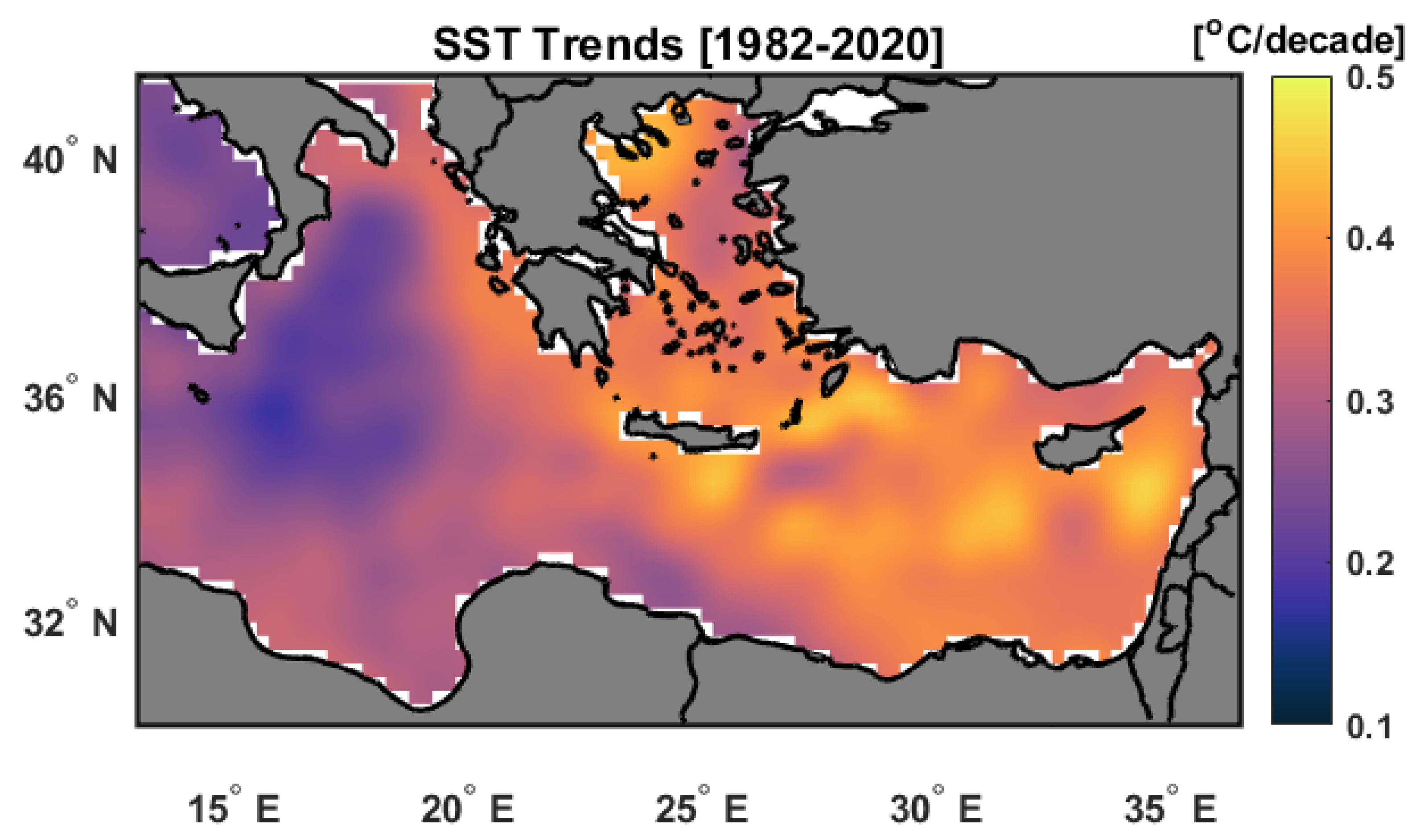
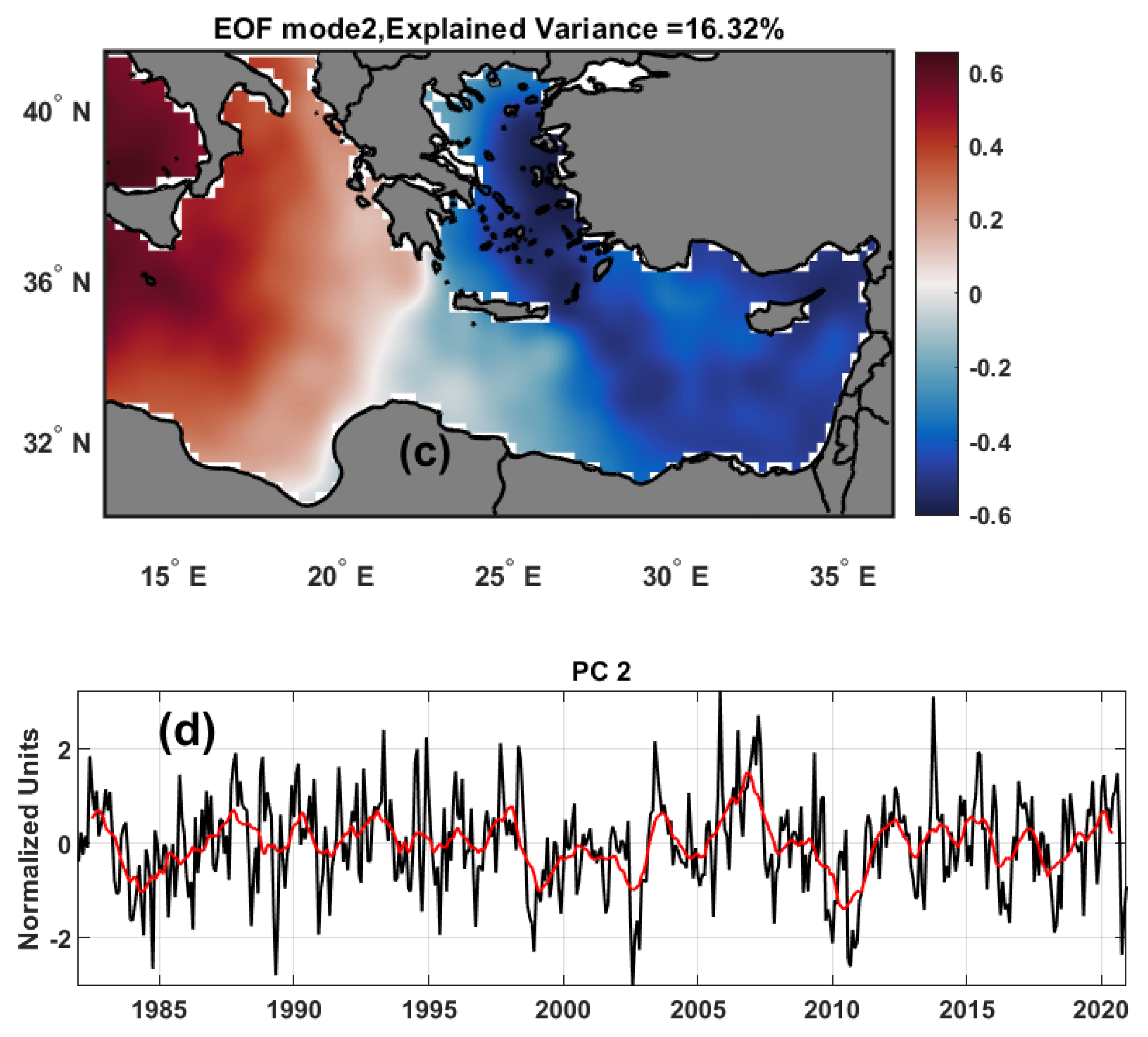
Trend and Inter-Annual Variability of SST

Figure 4 depicts a linear trend map after removing SST seasonality from 1982 to 2020. The original two-tailed modified Mann-Kendall test [26,27] was applied to the estimated trend at each grid point, the results indicate a statistically significant trend at the 95% confidence interval was observed over the whole region. High spatial variability of SST linear trend was observed over the EMED, ranging from 0.1 to 0.5 °C per decade. The basin average warming rate was about 0.33 ± 0.04 °C per decade. The higher values were found in the Aegean and Levantine Basin, while the lower values were observed in the Ionian and Tyrrhenian Sea.

The first three EOF modes of SST anomaly explain about 71% of the overall de-seasoned variance of the data. We only discuss the first two modes of EOF since the third mode describes less than 5% of the variance.

The spatial pattern of the first EOF1 mode, which accounts for approximately 50% of the overall deseasoned variance, is a positive anomaly over the entire region of the EMED (Figure 5a), suggesting an in-phase oscillation of the entire basin around the steady-state mean. The Ionian Sea and the Mersa Matruh gyre in the west of the Egyptian coast had the highest SST variability, while the Aegean Sea had the lowest variability, owing to the presence of strong and persistent Etesian winds over the Aegean Sea [35] and the input of Black Sea cold water inflow into the Aegean Sea [28]. The first temporal mode (PC1) reached its peak in the summer of 2003 (Figure 5b), which was the warmest summer over the study period, due to the strongest heat waves that hit the northern Europe. The highest negative peaks were observed in the winters of 1987 and 2019 in agreement with [46]. The lower peak values (i.e., cold periods) in the 1990s could be attributed to Mount Pinatubo’s eruption in the Philippines, which caused a cold air-temperature anomaly throughout the Middle East during the winter of 1992 As mentioned by [47], The spatial pattern of the second EOF2 mode (Explains 16% of the total variance) demonstrated a dipole in the study area (Figure 5c), with positive anomalies in the Ionian Sea and negative ones in the Levantine and Aegean basins. The temporal coefficient of the second mode (PC2) alternates between positive and negative patterns over the study period 1982–2020.

4. Spatial Description and Trends of the MHWs Main Characteristics from 1982 to 2020

Figure 6a–h depicts the spatial distribution and trends per decade of the EMED MHWs main characteristics, frequency, duration, (i_cum), and (i_max), which are overlaid with no significant values (p > 0.05) for the entire study period.

There was a clear decadal increase in MHW frequency in all EMED locations as demonstrated in Figure 6a,b. The frequency ranged from 1–2.5 counts with a maximum significant (p < 0.05) values > 2 events found in most of the Aegean and Levantine Seas, south of Crete and in front of the eastern coast of Libya. As shown in Figure 6b, the MHW frequency trend values were positively significant (p < 0.05) and ranged between 0 and 2.5 counts per decade. There were no significant (p > 0.05) changes in MHW frequency southeast of Crete, in front of Mersa Matruh city (see Figure 1a), and north of the Ionian Sea region (BiOS), which was previously described as a decadal reversal region in Section 3. The patterns of i_cum (trend) and mean duration (trend) are nearly identical, as shown in Figure 6c–f. The MHW mean duration increased significantly (p < 0.05) with values > 17 days with a trend of >10 days per decade in front of the Egyptian coast in the southeast of the Levantine Sea and off the Israeli coast, Figure 6d. No significant values (p > 0.05) are found in MHW duration at southeast of Crete, off Mersa Matruh city and the north Ionian Sea region. The maximum significant (p < 0.05) MHW i_cum values found in the Levantine Sea > 30 °C Days with a trend >15 °C Days per decade (Figure 6e,f). The MHW i_max patterns reveal maximum significant values > 1.5° with a trend > 0.25 °C throughout most of the Levantine Sea with an exception of south east corner and off Mersa Matruh city (see Figure 6g,h).

The authors found a strong relationship between the MHWs mean frequency and mean duration at each location over the study period (see, Figure 6a,c). The spatial pattern of mean MHW frequency and duration was highly negatively correlated (r = −0.76), which means the frequency was low where duration was long, and vice versa, example of similar analysis can be found in [3].

4.1. Description of the MHWs Mean Frequency Fields (1982–2020)

Figure 7a–d shows the spatial distribution of the EMED MHWs mean frequency events for the study periods. The P₁ mean MHW events are significantly < 2 counts over the whole EMED domain, Figure 7a. While during P₂ the MHW events have significantly increased up to 3 counts, Figure 7b. We found during P₃ that the Levantine basin has more significant (p < 0.05) MHW events (>3) than the Ionian and Aegean Seas, see Figure 7c. P₄ shows that most significant (p < 0.05) MHW events > 4 when compared to the other periods, Figure 7d.

4.2. Description of the MHWs Mean Duration (Days) Fields (1982–2020)

Figure 8a–d describes the spatial distribution of the EMED MHWs mean Duration (days) for the different periods, (P₁, P₂, P₃ and P₄). The spatial field for MHW mean duration over P₁ is mostly nonsignificant (p > 0.05) and less than 10 days for most of the domain. With an exception in the North Ionian area where the duration is significantly more than 18 days as shown in Figure 8a. For the most of the EMED domain, there was no significant difference in MHW mean duration (p > 0.05) during P₂. The MHW mean duration for P₂ ranges from 6.71 days to 20.53 days. We noticed during P₂ a high significant (p < 0.05) MHW mean duration value > 20 days located off South of Crete, see Figure 8b. P₃ and P₄ show an increase of significant MHW mean duration values throughout the EMED domain. For P₃, the MHW mean duration ranges from 9.07 days to 21.36 days, Figure 8c. The MHW mean duration pattern over the last decade shows greater significant values in the Levantine Sea. The least significant (p < 0.05) MHW mean duration is 10 days found in the South of the Aegean Sea, while it significantly exceeds 27 days off the Israeli coast as shown in Figure 8d. Finally, the findings revealed that the mean duration of MHWs has increased rapidly over the last two decades.

4.3. Description of the MHWs (i_cum) Fields (1982–2020)

Figure 9a–d presents the spatial distribution of the EMED MHWs mean cumulative intensity (°C days) for the different periods, (P₁, P₂, P₃ and P₄). The MHW i_cum, defined as the integral of intensity over the duration of the event [5], represents the MHW severity as mentioned by [48]. The mean spatial pattern for P₁ in Figure 9a shows non-significant values for most of the EMED basin. The highest P₁ significant (p < 0.05) value is >30 (°C days) and detected to the south of Italy in the Ionian Sea. Figure 9b demonstrates that the significant (p < 0.05) MHW i_cum values have increased for P₂. It ranges from 9.60 to 32.63 (°C days). The maximum MHW significant i_cum values for P₃ is >30 (°C days) and are located to the South of Cyprus and in the middle of the Ionian Sea, Figure 9c. The map of P₄ shows an increase of significant severity, which varies between 14.29 (°C days) and 39.51 (°C days) in the EMED domain. The highest significant MHW i_cum values > 35 (°C days) can be detected off the Israeli coast near the Shikmona anti-cyclonic gyre location as shown in Figure 9d. The Shikmona anti-cyclonic eddy was located the area between 34° E and 35° E longitudes and 33.5° N and 34.5° N latitudes [43,49,50].

4.4. Description of the MHWs (i_max) Fields (1982–2020)

Figure 10a–d shows the spatial distribution of the EMED MHWs i_max (°C) for the study periods. During P₁, the maximum significant (p < 0.05) mean MHW i_max was found throughout most of the Ionian Sea with values > 2 °C, Figure 10a. The significant MHW i_max values during P₂ vary between 1.33 °C at southeast Levantine basin and 2.45 °C at northeast Ionian basin near the Otranto strait, Figure 10b. The highest significant value for P₃ is 2.5 °C and is found north of the Aegean Sea, while the lowest significant value (1.31 °C) is found southeast of the Levantine Sea in front of the Egyptian coast. Among the entire study period, the MHW i_max spatial pattern for P₄ has the highest significant (p < 0.05). The MHW i_max values are significant during P₄ throughout the whole Levantine basin, Figure 10d. Figure 10d shows that the significant MHW i_max values range from 1.42 °C off Mersa Matruh to more than 2.5 °C in the northeast Aegean basin.

5. Extreme MHWs Events in the EMED over 1982–2020

Table 2. The EMED extreme significant (p < 0.05) MHW events characteristics (mean duration (Days), i_max (°C), i_mean (°C), and i_cum (°C days)) over the study period (1982–2020) with the corresponding MHW_onset, MHW_end, Longitude and Latitude in degrees where the highest events are highlighted in yellow color.

MHWonset	MHWend	Long.°E	Lat.°N	Mean Duration (Days)	imax (°C)	imean (°C)	icum (°C Days)
24-04-2013	08-05-2013	24.375	40.875	15	5.06	3.92	58.77
28-08-2020	31-12-2020	34.625	34.375	126	3.41	2.54	319.65
14-05-2020	20-05-2020	28.500	34.250	7	6.35	3.51	24.57

shows the significant EMED extreme MHW events characteristics (mean duration, i_max, i_mean, and i_cum) over the study period (1982–2020) with the corresponding MHW_onset, MHW_end, Longitude and Latitude. The maximum MHW i_mean was 3.92 °C in 2013, Figure 11a and lasted for 15 days (24 April–08 May) with an i_max of 5.06 °C and i_cum of 58.77 °C days. The most severe event (i_cum of 319.65 °C days) was still ongoing at the time of the analysis with 126 days, i_max of 3.41 °C and i_mean of 2.54 °C, Figure 11b. The most intense event occurred in 2020, with an i_max temperature of 6.35 °C and a duration of 7 days (this event will be discussed in detail in the following subsection). In general, the most extreme MHW significant events were mostly detected in 2020.

The EMED Most Intense [14–20 May 2020] MHW Event over the Study Period (1982–2020)

In this subsection, the authors will describe in detail the most significant intense event of 14–20 May 2020. We found the most significant intense MHW event located at longitude ~28.500° E and latitude ~34.250° N south of Rhodes. Two more MHW significant events were discovered to be associated with the most intense main event, according to our analysis. The three significant events occur in the Levantine basin. It is critical in our research to assist in identifying and quantifying the main atmospheric causes of these extreme events.

Table 3. The EMED most intense (14–20 May 2020) MHW events characteristics (mean duration (Days), i_max (°C), i_mean (°C), i_cum (°C days)), wind stress magnitude (N/m²), 2 m air temperature (°C) and mean sea level pressure (mb) with the corresponding Longitude and Latitude in degrees.

Long.° E	Lat.° N	imax (°C)	imean (°C)	icum (°C Days)	Wind Stress Magnitude (N/m2)	2m Air Temp. (°C)	Msl Pressure (mb)
28.500	34.250	6.35	3.51	24.57	2.7 × 10−4	27.71	1015.2
24.625	35.875	5.66	3.25	22.78	6.2 × 10−5	27.69	1014.5
34.125	36.125	4.74	3.34	26.71	1.3 × 10−3	26.06	1014.1

demonstrates the EMED most intense [14–20 May 2020] MHW significant event characteristics, including duration, i_max, i_mean, i_cum, wind stress magnitude, 2m air temperature and mean sea level pressure. The i_max for the four events are 6.35, 5.66, 4.74, and 2.95 °C, respectively.

Figure 12a shows the SST anomaly event map created by subtracting the historical climatological mean value at each grid from the mean temperature 14–20 May 2020 at the same location (grid). The description of temporal evolution of the SST most intense MHW event based on threshold 90th percentile and SST climatology are shown in Figure 12b. The spatial distribution patterns of the wind stress vectors combined with magnitude, 2 m mean air temperature and mean sea level pressure of ERA5 were chosen at the same time and location as the SST anomaly analysis, as shown in Figure 12c–e. We can see an interesting relationship between the SST anomaly, wind stress, and 2 m mean air temperature fields. We observed a reduction in the magnitude of wind stress fields (less than 0.001 N/m²) at the same locations as the most intense MHW events (see Figure 12c and Table 3). The comparison of wind stress fields and SST anomaly fields revealed that MHW extreme events are related to wind stress reduction, which is consistent with the findings of [14,15,16,18]. Another intriguing parallel is found between the SST anomaly and the 2 m mean air temperature patterns. High air temperature values (>25 °C) were found at the same locations as the MHW extreme events, as shown in Figure 12d and Table 3. Furthermore, we observed a very persistent ridge of high atmospheric pressure >1014 mb over the MHW extreme events locations in the EMED as shown in Figure 12e and Table 3. In conclusion, the atmospheric conditions, such as, mean sea level pressure, wind stress, and air temperature, may be linked to MHWs existence, Figure 12c–e.

6. Discussion

According to our SST climatology analysis (Figure 2 and Figure 3), the maximum values over the four decades were detected during the last decade, which agrees with [19,35,36]. Table 1 have showed that the last decade was the warmest decade by about 0.94 °C during the entire 1982–2020 study period in agreement with [51,52]. During the last decade, the SST anomaly patterns revealed a warming of about 0.10 to 0.50 °C over the northern EMED basin, with the exception of some parts of the north Ionian Sea (Figure 3d). The authors have attributed this to the effect of BiOS which is responsible for decadal reversals of the Ionian basin-wide circulation as mentioned by [37,38,39,40,41]. The maximum SST anomaly for the last decade was 0.50 °C in the northwest Aegean Sea, while the minimum value was −0.50 °C along EMED’s southwestern coast (Figure 3d).

The authors have discovered a high spatial variability of SST linear trend over the EMED, ranging from 0.1 to 0.5 °C per decade (Figure 4). The basin average warming rate was about 0.33 ± 0.04 °C per decade. Over the last twenty years, several SST studies for the Mediterranean and the EMED region were published, addressing trends and changes in ocean surface temperature [6,19,28,35,52,53,54,55,56,57,58]. Ref. [53] have observed a trend of 0.3 °C per decade in the western basin and 0.5 °C per decade in the eastern basin over the period from 1985 to 2006. Similar results were recorded in [28], with an average mean warming rate of around 0.37 °C per decade for the whole Mediterranean basin during 1985–2008, and 0.26 °C per decade and 0.42 °C per decade for the western and eastern sub-basins, respectively. Over a 25-year (1993–2017), the warming rate in the Mediterranean was about 0.36 °C per decade, which was highly correlated with sea level trend, especially in the EMED [52]. According to [35], the annual warming trend for the deseasonalized Mediterranean global averaged SST was 0.36 °C per decade over the period 1982–2016. More recently, studies with longer time series, such as [19], estimated a 0.35 °C per decade warming for the global Mediterranean basin for the 38-year period 1982–2019. Figure 5 have revealed the highest negative peaks were observed in the winters of 1987 and 2019 in accordance with [46], The lower peak values (i.e., cold periods) in the 1990s could be attributed to the eruption of Mount Pinatubo in the Philippines, which caused a cold air-temperature anomaly throughout the Middle East during the winter of 1992, as stated by [47].

We have shown in Figure 6 the spatial distribution and trends per decade of the MHWs main characteristics (mean frequency, duration, (i_cum) and (i_max)) overlaid with no significant values (p > 0.05) for the entire study period. According to Figure 6c–f we found the patterns of i_cum (trend) and mean duration (trend) were nearly identical. The MHW mean duration has increased significantly (p < 0.05) with values > 17 days with a trend of > 10 days per decade in front of the Egyptian coast in the southeast of the Levantine Sea and off the Israeli coast (Figure 6d). No significant values (p > 0.05) were found in MHW duration at southeast of Crete, off Mersa Matruh city and the north Ionian Sea region. This could be attributed to the accuracy and precision of SST NOAA AVHRR data near coastlines, as described by [59,60]. According to their research, the accuracy and precision of Earth Observation (EO) SST data at the coastline are not well defined. According to Figure 7, the Levantine basin has more significant (p < 0.05) MHW events (>4) in the last decade than the Ionian and Aegean Seas.

In the last decade, the highest significant MHW (p < 0.05) duration > 27 days and i_cum values > 35 (°C days) were detected off the Israeli coast (Figure 8d and Figure 9d), near the Shikmona anti-cyclonic gyre location [43,50]. The MHW i_max spatial distribution pattern were significant (p < 0.05) throughout the entire Levantine basin over the last decade as demonstrated in Figure 10d. The significant MHW i_max values have ranged from 1.42 °C off Mersa Matruh to more than 2.5 °C in the northeast Aegean basin, as presented in Figure 10d. An extreme MHW event was discovered in 2013, with the maximum MHW i_mean temperature of 3.92 °C and lasted 15 days (24 April–08 May) with an i_max of 5.06 °C and i_cum of 58.77 °C days (Figure 11a and Table 2). While, the most severe event (i_cum of 319.65 °C days) was still ongoing at the time of the analysis with 126 days, i_max of 3.41 °C and i_mean of 2.54 °C, Figure 11b. The most significant intense MHW event was located south of Rhodes at longitude ~28.500° E and latitude ~34.250° N and was associated with another two extreme events located in Levantine basin, that occurred simultaneously in 14–20 May 2020 with very high intensities (Figure 12a and Table 3). At the same locations as the most intense MHW events, we have observed a reduction in the magnitude of wind stress fields (less than 0.001 N/m²) (see Figure 12c and Table 3). We have concluded that the MHW extreme events are related to the wind stress reduction in agreement with [14,15,16,18].

7. Conclusions

This study has quantified the SST interannual variability, trends, and spatial distribution of main MHW characteristics in the EMED over 39 years (1982–2020).

Some specific hotspot areas in the Mediterranean Sea as described by [61] such as Aegean, north Levantine and north Ionian have been recorded as the highest SST anomaly patterns during P₄ (2011–2020) which agrees with [18]. During last decade (P₄ (2011–2020)), the northern EMED basin’s mean SST anomaly was nearly 1.00 °C higher than the southern one. The minimum SST anomaly value found −0.50 °C and was located on the southwestern coast of EMED in agreement with [18]. This could be due to upwelling associated with the Rhodes cyclonic gyre in the northern EMED basin, as mentioned in [42].

The SST EOF analysis revealed that the Ionian Sea had the highest interannual variability, while the Aegean had the lowest.

Over the entire study period, there was a clear decadal increase in MHW frequency in all EMED locations. The MHW frequency trend values were significantly (p < 0.05) positive. The correlation analysis between the mean MHWs spatial distribution of duration and frequency revealed a strong negative relationship, which was consistent with the findings of [3]. The authors found that the mean MHW frequency and duration increased by 40% and 15%, respectively

We have characterized trends and variability of MHWs for the EMED from 1982 to 2020 based on satellite NOAA OI SST V2.1 data and a unified MHW framework. We have shown that between 1982 and 2020, on EMED average, MHW frequency trend increased by 1.2 events per decade and the average MHW i_cum trend increased by 5.4 °C days.

The MHW main characteristics patterns over the last decade have shown greater significant values in most of the Levantine Sea. There were no significant (p > 0.05) found in the MHW main characteristics at southeast of Crete, off Mersa Matruh city and the north Ionian Sea region over the entire the study period.

The authors have showed the significant EMED extreme MHW events characteristics (mean duration, i_max, i_mean, and i_cum) over the study period (1982–2020). During these extreme events, there was a similarity in the SST anomaly, wind stress, and 2 m mean air temperature fields. We observed a reduction in the magnitude of wind stress fields (less than 0.001 N/m²) at the same locations as the most intense MHW events. High air temperature values (>25 °C) have been linked to the locations of MHW extreme events. We concluded that atmospheric conditions such as mean sea level pressure, wind stress, and air temperature could be related to the existence of MHW.

In the future, we should focus more on the anthropogenic factors that contribute to the increasing severity and recurrence of MHW events. Furthermore, possible MHW links to different climatic and atmospheric indices [13,62,63,64] such as North Atlantic Oscillations (NAO), East Atlantic (EA), East Atlantic–West Russia (EAW), Mediterranean Oscillation (MO) and North-Sea Caspian Pattern (NCP). There is a lot of speculation about what caused the weather pattern we saw during this most severe MHW event. Was it just a coincidental occurrence? More information about the detection, characterization, impact assessment, and prediction of MHWs could be obtained.

References

1. Frölicher, T.L.; Laufkötter, C. Emerging risks from marine heat waves. Nat. Commun. 2018, 9, 650. [Google Scholar] [CrossRef]
2. Manta, G.; de Mello, S.; Trinchin, R.; Badagian, J.; Barreiro, M. The 2017 record marine heatwave in the Southwestern Atlantic shelf. Geophys. Res. Lett. 2018, 45. [Google Scholar] [CrossRef]
3. Oliver, E.C.J.; Donat, M.G.; Burrows, M.T.; Moore, P.J.; Smale, D.A.; Alexander, L.V.; Benthuysen, J.A.; Feng, M.; Gupta, A.S.; Hobday, A.J.; et al. Longer and more frequent marine heatwaves over the past century. Nat. Commun. 2018, 9, 1324. [Google Scholar] [CrossRef]
4. Hobday, A.J.; Alexander, L.V.; Perkins, S.E.; Smale, D.A.; Straub, S.C.; Oliver, E.C.; Benthuysen, J.A.; Burrows, M.T.; Donat, M.G.; Feng, M.; et al. A hierarchical approach to defining marine heatwaves. Prog. Oceanogr. 2016, 141, 227–238. [Google Scholar] [CrossRef] [Green Version]
5. Hobday, A.J.; Oliver, E.C.; Gupta, A.S.; Benthuysen, J.A.; Burrows, M.T.; Donat, M.G.; Holbrook, N.J.; Moore, P.J.; Thomsen, M.S.; Wernberg, T.; et al. Categorizing and naming marine heatwaves. Oceanography 2018, 31, 162–173. [Google Scholar] [CrossRef] [Green Version]
6. Strub, P.T.; James, C.; Montecino, V.; Rutllant, J.A.; Blanco, J.L. Ocean circulation along the southern Chile transition region (38°–46°S): Mean, seasonal and interannual variability, with a focus on 2014–2016. Prog. Oceanogr. 2019, 172, 159–198. [Google Scholar] [CrossRef]
7. Holbrook, N.J.; Scannell, H.A.; Gupta, A.S.; Benthuysen, J.A.; Feng, M.; Oliver, E.C.J.; Alexander, L.V.; Burrows, M.T.; Donat, M.G.; Hobday, A.J.; et al. A global assessment of marine heatwaves and their drivers. Nat. Commun. 2019, 10, 2624. [Google Scholar] [CrossRef] [PubMed]
8. Jacox, M.G. Marine heatwaves in a changing climate. Nature 2019, 571, 485–487. [Google Scholar] [CrossRef] [Green Version]
9. Garrabou, J.; Coma, R.; Bensoussan, N.; Bally, M.; Chevaldonné, P.; Cigliano, M.; Diaz, D.; Harmelin, J.G.; Gambi, M.; Kersting, D. Mass mortality in Northwestern Mediterranean rocky benthic communities: Effects of the 2003 heat wave. Glob. Chang. Biol. 2009, 15, 1090–1103. [Google Scholar] [CrossRef]
10. Marba, N.; Duarte, C.M. Mediterranean warming triggers seagrass (posidonia oceanica) shoot mortality. Glob. Chang. Biol. 2010, 16, 2366–2375. [Google Scholar] [CrossRef]
11. Malanotte-Rizzoli, P. Introduction to special section: Physical and biochemical evolution of the eastern Mediterranean in the 1990s (PBE). J. Geophys. Res. 2003, 108, 8100. [Google Scholar] [CrossRef] [Green Version]
12. Borzelli, G.L.E.; Gacic, M.; Cardin, V.; Civitarese, G. Eastern Mediterranean Transient and Reversal of the Ionian Sea Circulation. Geophys. Res. Lett. 2009, 36, L15108. [Google Scholar] [CrossRef]
13. Pinardi, N.; Cessi, P.; Borile, F.; Wolfe, C.L.P. The Mediterranean Sea overturning circulation. J. Phys. Oceanogr. 2019, 49, 1699–1721. [Google Scholar] [CrossRef]
14. Grazzini, F.; Viterbo, P. Record-breaking warm sea surface temperature of the Mediterranean Sea. ECMWF Newslett. 2003, 98, 30–31. [Google Scholar]
15. Sparnocchia, S.; Schiano, M.; Picco, P.; Bozzano, R.; Cappelletti, A. The anomalous warming of summer 2003 in the surface layer of the Central Ligurian Sea (Western Mediterranean). Ann. Geophys. 2006, 24, 443–452. [Google Scholar] [CrossRef]
16. Olita, A.; Sorgente, R.; Natale, S.; Ribotti, A.; Bonanno, A.; Patti, B. Effects of the 2003 European heatwave on the Central Mediterranean Sea: Surface fluxes and the dynamical response. Ocean Sci. 2007, 3, 273–289. [Google Scholar] [CrossRef] [Green Version]
17. Mavrakis, A.F.; Tsiros, I.X. The abrupt increase in the Aegean Sea surface temperature during the June 2007 southeast Mediterranean heatwave-a marine heatwave event? Weather 2018, 74, 201–207. [Google Scholar] [CrossRef]
18. Darmaraki, S.; Somot, S.; Sevault, F.; Nabat, P.; Narvaez, W.D.C.; Cavicchia, L.; Djurdjevic, V.; Li, L.; Sannino, G.; Sein, D.V. Future evolution of Marine Heatwaves in the Mediterranean Sea. Clim. Dyn. 2019, 53, 1371–1392. [Google Scholar] [CrossRef] [Green Version]
19. Pastor, F.; Valiente, J.A.; Khodayar, S. A Warming Mediterranean: 38 Years of Increasing Sea Surface Temperature. Remote Sens. 2020, 12, 2687. [Google Scholar] [CrossRef]
20. Pinardi, N.; Zavatarelli, M.; Arneri, E.; Crise, A.; Ravaioli, M. The physical, sedimentary and ecological structure and variability of shelf areas in the Mediterranean Sea. In The Sea; Robinson, A.R., Brink, K.H., Eds.; Harvard University Press: Cambridge, MA. USA, 2005; Volume 14B, Chapter 32; pp. 1245–1331. [Google Scholar]
21. Nagy, H.; Elgindy, A.; Pinardi, N.; Zavatarelli, M.; Oddo, P. A nested pre-operational model for the Egyptian shelf zone: Model configuration and validation/calibration. J. Dyn. Atmos. Ocean. 2017, 80, 75–96. [Google Scholar] [CrossRef]
22. Reynolds, R.W.; Smith, T.M.; Liu, C.; Chelton, D.B.; Casey, K.S.; Schlax, M.G. Daily high-resolution-blended analyses for sea surface temperature. J. Clim. 2007, 20, 5473–5496. [Google Scholar] [CrossRef]
23. Thomson, R.E.; Emery, W.J. Data Analysis Methods in Physical Oceanography, 3rd ed.; Elsevier Inc.: Amsterdam, The Netherlands, 2014; ISBN 9780123877833. [Google Scholar]
24. Arafeh-Dalmau, N.; Montaño-Moctezuma, G.; Martínez, J.A.; Beas-Luna, R.; Schoeman, D.S.; Torres-Moye, G. Extreme Marine Heatwaves Alter Kelp Forest Community Near Its Equatorward Distribution Limit. Front. Mar. Sci. 2019, 6, 499. [Google Scholar] [CrossRef]
25. Wilks, D.S. Statistical Methods in the Atmospheric Sciences; Academic Press: Cambridge, MA, USA, 2011; ISBN 0123850223. [Google Scholar]
26. Hamed, K.H.; Ramachandra Rao, A. A modified Mann-Kendall trend test for autocorrelated data. J. Hydrol. 1998, 204, 182–196. [Google Scholar] [CrossRef]
27. Wang, F.; Shao, W.; Yu, H.; Kan, G.; He, X.; Zhang, D.; Ren, M.; Wang, G. Re-evaluation of the Power of the Mann-Kendall Test for Detecting Monotonic Trends in Hydrometeorological Time Series. Front. Earth Sci. 2020, 8, 14. [Google Scholar] [CrossRef]
28. Skliris, N.; Sofianos, S.; Gkanasos, A.; Mantziafou, A.; Vervatis, V.; Axaopoulos, P.; Lascaratos, A. Decadal scale variability of sea surface temperature in the Mediterranean Sea in relation to atmospheric variability. Ocean Dyn. 2012, 62, 13–30. [Google Scholar] [CrossRef]
29. Trenberth, K.E. Signal versus noise in the Southern Oscillation. Monthly. Weather Rev. 1984, 112, 326–333. [Google Scholar] [CrossRef] [Green Version]
30. Carlson, D.F.; Yarbo, L.A.; Scolaro, S.; Poniatowski, M.; Absten, V.M.; Carlson, P.R., Jr. Sea surface temperatures and seagrass mortality in Florida Bay: Spatial andtemporal patterns discerned from MODIS and AVHRR data. Remote Sens. Environ. 2018, 208, 171–188. [Google Scholar] [CrossRef]
31. Zhao, Z.; Marin, M. A MATLAB toolbox to detect and analyze marine heatwaves. J. Open Source Softw. 2019, 4, 1124. [Google Scholar] [CrossRef]
32. Hersbach, H.; Bell, B.; Berrisford, P.; Hirahara, S.; Horányi, A.; Muñoz-Sabater, J.; Nicolas, J.; Peubey, C.; Radu, R.; Schepers, D.; et al. The ERA5 global reanalysis. Q. J. R. Meteorol. Soc. 2020, 146, 1999–2049. [Google Scholar] [CrossRef]
33. Nagy, H.; Lyons, K.; Nolan, G.; Cure, M.; Dabrowski, T. A Regional Operational Model for the North East Atlantic: Model Configuration and Validation. J. Mar. Sci. Eng. 2020, 8, 673. [Google Scholar] [CrossRef]
34. Hellerman, S.; Rosenstein, M. Normal monthly wind stress over the world ocean with error estimates. Phys. Oceanogr. 1983, 13, 1093–1104. [Google Scholar] [CrossRef] [Green Version]
35. Pastor, F.; Valiente, J.A.; Palau, J.L. Sea surface temperature in the Mediterranean: Trends and spatial patterns (1982–2016). Pure Appl. Geophys. 2018, 175, 4017–4029. [Google Scholar] [CrossRef] [Green Version]
36. El-Geziry, T.M. Long-term changes in sea surface temperature (SST) within the southern Levantine Basin. Acta Oceanol. Sin. 2021, 40, 27–33. [Google Scholar] [CrossRef]
37. Gacic, M.; Civitarese, G.; EusebiBorzelli, G.L.; Kovacevic, V.; Poulain, P.M.; Theocharis, A.; Menna, M.; Catucci, A.; Zarokanellos, N. On the relationship between the decadal oscil-lations of the Northern Ionian Sea and the salinity distributions in the Eastern Mediterranean. J. Geophys. Res. 2011, 116, C12002. [Google Scholar] [CrossRef]
38. Gacic, M.; Civitarese, G.; Kovacevic, V.; Ursella, L.; Bensi, M.; Menna, M.; Cardin, V.; Poulain, P.M.; Cosoli, S.; Notarstefano, G.; et al. Extreme winter 2012 in the Adriatic: An example of climatic effect on the BiOS rhythm. Ocean Sci. 2014, 10, 513–522. [Google Scholar] [CrossRef] [Green Version]
39. Mkhinini, N.; Coimbra, A.L.S.; Stegner, A.; Arsouze, T.; Taupier-Letage, I.; Béranger, K. Long-lived mesoscale eddies in the eastern Mediterranean Sea: Analysis of 20 years of AVISO geostrophic velocities. J. Geophys. Res. Ocean. 2014, 119, 8603–8626. [Google Scholar] [CrossRef]
40. Nagy, H.; Di-Lorenzo, E.; El-Gindy, E. The Impact of Climate Change on Circulation Patterns in the Eastern Mediterranean Sea Upper Layer Using Med-ROMS Model. Prog. Oceanogr. 2019, 175, 244. [Google Scholar] [CrossRef]
41. Rubino, A.; Gačić, M.; Bensi, M.; Kovačević, V.; Malačič, V.; Menna, M.; Negretti, M.E.; Sommeria, J.; Zanchettin, D.; Barreto, R.V.; et al. Experimental evidence of long-term oceanic circulation reversals without wind influence in the North Ionian Sea. Sci. Rep. 2020, 10, 1905. [Google Scholar] [CrossRef]
42. Pinardi, N.; Masetti, E. Variability of the large-scale General Circulation of the Mediterranean Sea from observation and modeling: A review. Palaeogeogr. Palaeoclimatol. Palaeoecol. 2000, 158, 153–173. [Google Scholar] [CrossRef]
43. Amitai, Y.; Lehahn, Y.; Lazar, A.; Heifetz, E. Surface circulation of the eastern Mediterranean Levantine basin: Insights from analyzing 14 years of satellite altimetry data. J. Geophys. Res. 2010, 115, C10058. [Google Scholar] [CrossRef]
44. Carniel, S.; Bonaldo, D.; Benetazzo, A.; Bergamasco, A.; Boldrin, A.; Falcieri, F.M.; Sclavo, M.; Trincardi, F.; Falcieri, F.M.; Langone, L.; et al. Off-Shelf Fluxes across the Southern Adriatic Margin: Factors Controlling Dense Water-Driven Transport Phenomena. Mar. Geol. 2016, 375, 44–63. [Google Scholar] [CrossRef]
45. Chhak, K.; Di Lorenzo, E. Decadal variations in the California Current upwelling cells. Geophys. Res. Lett. 2007, 34. [Google Scholar] [CrossRef] [Green Version]
46. Tolika, K.; Maheras, P.; Pytharoulis, I.; Anagnostopoulou, C. The anomalous low and high temperatures of 2012 over Greece—An explanation from a meteorological and climatological perspective. Nat. Hazards Earth Syst. Sci. 2014, 14, 501–507. [Google Scholar] [CrossRef] [Green Version]
47. Genin, A.; Lazar, B.; Brenner, S. Vertical mixing and coral death in the Red Sea following the eruption of Mount Pinatubo. Nature 1995, 377, 507–510. [Google Scholar] [CrossRef]
48. Galli, G.; Solidoro, C.; Lovato, T. Marine heat waves hazard 3D maps, and the risk for low motility organisms in a warming Mediterranean Sea. Front. Mar. Sci. 2017, 4, 136. [Google Scholar] [CrossRef] [Green Version]
49. Brenner, S. Structure, and evolution of warm core eddies in the Eastern Mediterranean Levantine Basin. J. Geophys. Res. 1989, 94, 12593–12602. [Google Scholar] [CrossRef]
50. Brenner, S. Long term evolution and dynamics of a persistent warm Core eddies in the Eastern Mediterranean Sea. J. Deep Sea Res. 1993, 40, 1193–1206. [Google Scholar] [CrossRef]
51. Minnett, P.J.; Azcárate, A.A.; Chin, T.M.; Corlett, G.K.; Gentemann, C.L.; Karagali, I.; Li, X.; Marsouin, A.; Marullo, S.; Maturi, E.; et al. Half a century of satellite remote sensing of sea-surface temperature. Remote Sens. Environ. 2019, 233, 111366. [Google Scholar] [CrossRef]
52. Mohamed, B.; Abdallah, A.M.; Din, K.A.E.; Nagy, H.; Shaltout, M.A. Inter-annual variability and trends of sea level and sea surface temperature in the mediterranean sea over the last 25 years. Pure Appl. Geophys. 2019, 176, 3787–3810. [Google Scholar] [CrossRef]
53. Nykjaer, L. Mediterranean sea surface warming 1985–2006. Clim. Res. 2009, 39, 11–17. [Google Scholar] [CrossRef]
54. Rayner, N.A.; Brohan, P.; Parker, D.E.; Folland, C.K.; Kenndy, J.J.; Vanicek, M.; Ansell, T.J.; Tett, S.F.B. Improved analysis of changes and uncertainties in sea surface temperature measured in situ since the mid-ninteenth century: The HadSST2 dataset. J. Clim. 2006, 19, 446–469. [Google Scholar] [CrossRef] [Green Version]
55. Marullo, S.; Artale, V.; Santoleri, R. The SST multidecadal variability in the Atlantic-Mediterranean region and its relation to AMO. J. Clim. 2011, 24, 4385–4401. [Google Scholar] [CrossRef]
56. Banzon, V.; Smith, T.M.; Chin, T.M.; Liu, C.; Hankins, W. A long-term record of blended satellite and in situ sea-surface temperature for climate monitoring, modeling, and environmental studies. Earth Syst. Sci. Data 2016, 8, 165–176. [Google Scholar] [CrossRef] [Green Version]
57. Fiedler, E.K.; McLaren, A.; Banzon, V.; Brasnett, B.; Ishizaki, S.; Kennedy, J.; Rayner, N.; Jones, J.R.; Corlett, G.; Merchant, C.J.; et al. Intercomparison of long-term sea surface temperature analyses using the GHRSST Multi-Product Ensemble (GMPE) system. Remote Sens. Environ. 2019, 222, 18–33. [Google Scholar] [CrossRef] [Green Version]
58. López García, M.J. SST Comparison of AVHRR and MODIS Time Series in the Western Mediterranean Sea. Remote Sens. 2020, 12, 2241. [Google Scholar] [CrossRef]
59. Brewin, R.J.W.; de Mora, L.; Billson, O.; Jackson, T.; Russell, P.; Brewin, T.G.; Shutler, J.; Miller, P.I.; Taylor, B.H.; Smyth, T.; et al. Evaluating operational AVHRR sea surface temperature data at the coastline using surfers. Estuar. Coast. Shelf Sci. 2017, 196, 276–289. [Google Scholar] [CrossRef]
60. Brewin, R.J.W.; Smale, D.A.; Moore, P.J.; Dall’Olmo, G.; Miller, P.I.; Taylor, B.H.; Smyth, T.J.; Fishwick, J.R.; Yang, M. Evaluating Operational AVHRR Sea Surface Temperature Data at the Coastline Using Benthic Temperature Loggers. Remote Sens. 2018, 10, 925. [Google Scholar] [CrossRef] [Green Version]
61. Giorgi, F. Climate change hot-spots. Geophys. Res. Lett. 2006, 33. [Google Scholar] [CrossRef]
62. Kutiel, H.; Benaroch, Y. North Sea-Caspian Pattern (NCP)—An upper level atmospheric teleconnection aecting the Eastern Mediterranean: Identication and definition. Theor. Appl. Climatol. 2002, 71, 17–28. [Google Scholar] [CrossRef]
63. Brunetti, M.; Kutiel, H. The relevance of the North-Sea Caspian Pattern (NCP) in explaining temperature variability in Europe and the Mediterranean. Nat. Hazards Earth Syst. Sci. 2011, 11, 2881–2888. [Google Scholar] [CrossRef] [Green Version]
64. Criado-Aldeanueva, F.; Soto-Navarro, J. Climatic Indices over the Mediterranean Sea: A Review. Appl. Sci. 2020, 10, 5790. [Google Scholar] [CrossRef]
Figure 1. (a) The Eastern Mediterranean Sea with the main geographic features (e.g., Basins) where, the solid red square is the position of Mersa Matruh City, the solid blue circle is the position of Crete, the solid green circle is the position of Rhodes, the solid yellow circle is the position of Cyprus and the solid continuous red lines delineate the boundaries between EMED basins. (b) Bathymetry according to GEBCO bathymetric dataset (https://www.gebco.net/ (accessed on 20 March 2021)) with 10 m as the minimum depth.
Jmse 09 00643 g001aJmse 09 00643 g001b
Figure 2. Temporal evolution of the basin averaged plotted SST in (°C) where P1 (1982–1990) in continuous blue line, P2 (1991–2000) in continuous green line, P3 (2001–2010) in continuous cyan line and P4 (2011–2020) in continuous red line.
Jmse 09 00643 g002
Figure 3. The EMED SST climatological anomaly maps where (a) P1 (1982–1990), (b) P2 (1991–2000), (c) P3 (2001–2010), and (d) P4 (2011–2020). Anomaly maps are calculated by subtracting the climatological mean value over (1982–2020) from each period value (P1, P2, P3 and P4) at the same location (grid).
Jmse 09 00643 g003
Figure 4. Spatial trend map of SST anomaly over the EMED from AVHRR during 1982–2020, after the seasonal cycle was removed at each grid point.
Jmse 09 00643 g004
Figure 5. (a) Spatial distribution for the principal (EOF) component (PC1). (b) Temporal evolution for EOF (PC1) in normalised variance units. (c) Spatial distribution for the second (EOF) component (PC2). (d) Temporal evolution for EOF (PC2) in normalised variance units; for the EMED SST anomaly covering the period from 1982 to 2020. In (b,d), the deseasoned monthly PCs time series is shown in continuous black lines, and the low passed using a 13-month running mean is shown in continuous red lines.
Jmse 09 00643 g005aJmse 09 00643 g005b
Figure 6. The Marine heatwave properties over the 1982–2020 period, averaged time series of (a) mean MHW frequency (Count), (b) MHW frequency trend (Count/Decade), (c) mean MHW duration (Days), (d) MHW duration trend (Days/Decade), (e) mean MHW (icum) (°C Days), (f) MHW (icum) trend (°C Days/Decade), (g) mean MHW (imax) (°C), (h) MHW (imax) trend (°C/Decade), and the black dots indicate the change is not significantly different (p > 0.05). Where, the solid red square is the position of Mersa Matruh City, the solid blue circle is the position of Crete, the solid green circle is the position of Rhodes, and the solid yellow circle is the position of Cyprus.
Jmse 09 00643 g006
Figure 7. The EMED MHWs mean frequency (Count) for (a) P1 (1982–1990), (b) P2 (1991–2000), (c) P3 (2001–2010) and (d) P4 (2011–2020), and the black dots indicate the change is not significantly different (p > 0.05).
Jmse 09 00643 g007
Figure 8. The EMED MHWs mean duration (days) for (a) P1 (1982–1990), (b) P2 (1991–2000), (c) P3 (2001–2010) and (d) P4 (2011–2020), and the black dots indicate the change is not significantly different (p > 0.05).
Jmse 09 00643 g008
Figure 9. The EMED MHWs mean cumulative intensity (°C days) for (a) P1 (1982–1990), (b) P2 (1991–2000), (c) P3 (2001–2010) and (d) P4 (2011–2020), and the black dots indicate the change is not significantly different (p > 0.05).
Jmse 09 00643 g009aJmse 09 00643 g009b
Figure 10. The EMED MHWs imax (°C) for (a) P1 (1982–1990), (b) P2 (1991–2000), (c) P3 (2001–2010) and (d) P4 (2011–2020), and the black dots indicate the change is not significantly different (p > 0.05).
Jmse 09 00643 g010
Figure 11. The EMED extreme MHW significant events over the study period (1982–2020), The SST climatology from NOAA OI SST for the detection of MHWs (blue), 90th percentile MHW threshold (green), and SST time series (black) for each MHW. The pink filled area indicates the period associated with the identified MHW, where (a) MHW extreme highest mean intensity event (imean 3.92 °C) (24-04-2013 to 08-05-2013), (b) MHW extreme highest cumulative intensity event (icum 319.65 °C days) (28-08-2020—ongoing).
Jmse 09 00643 g011
Figure 12. The EMED most significant intense (14–20 May 2020) MHW events over the study period (1982–2020), where, (a) MHW mean SST anomaly °C. (b) SST climatology from NOAA OI SST for the detection of MHWs (blue), 90th percentile MHW threshold (green), and SST time series (black) for each MHW. The pink filled area indicates the period associated with the identified MHW event. (c) Wind stress vectors combined with magnitude for the MHW in N/m2 based on ERA5 hourly data. (d) 2 m mean air temperature °C based on ERA5 hourly data. (e) Mean sea level pressure (mb) based on ERA5 hourly data.
Jmse 09 00643 g012