
Physical Modelling of Offshore Wind Turbine Foundations for TRL (Technology Readiness Level) Studies

 ,
, 
 ,
,  ,
,  ,
,  ,
,  ,
,
Abstract
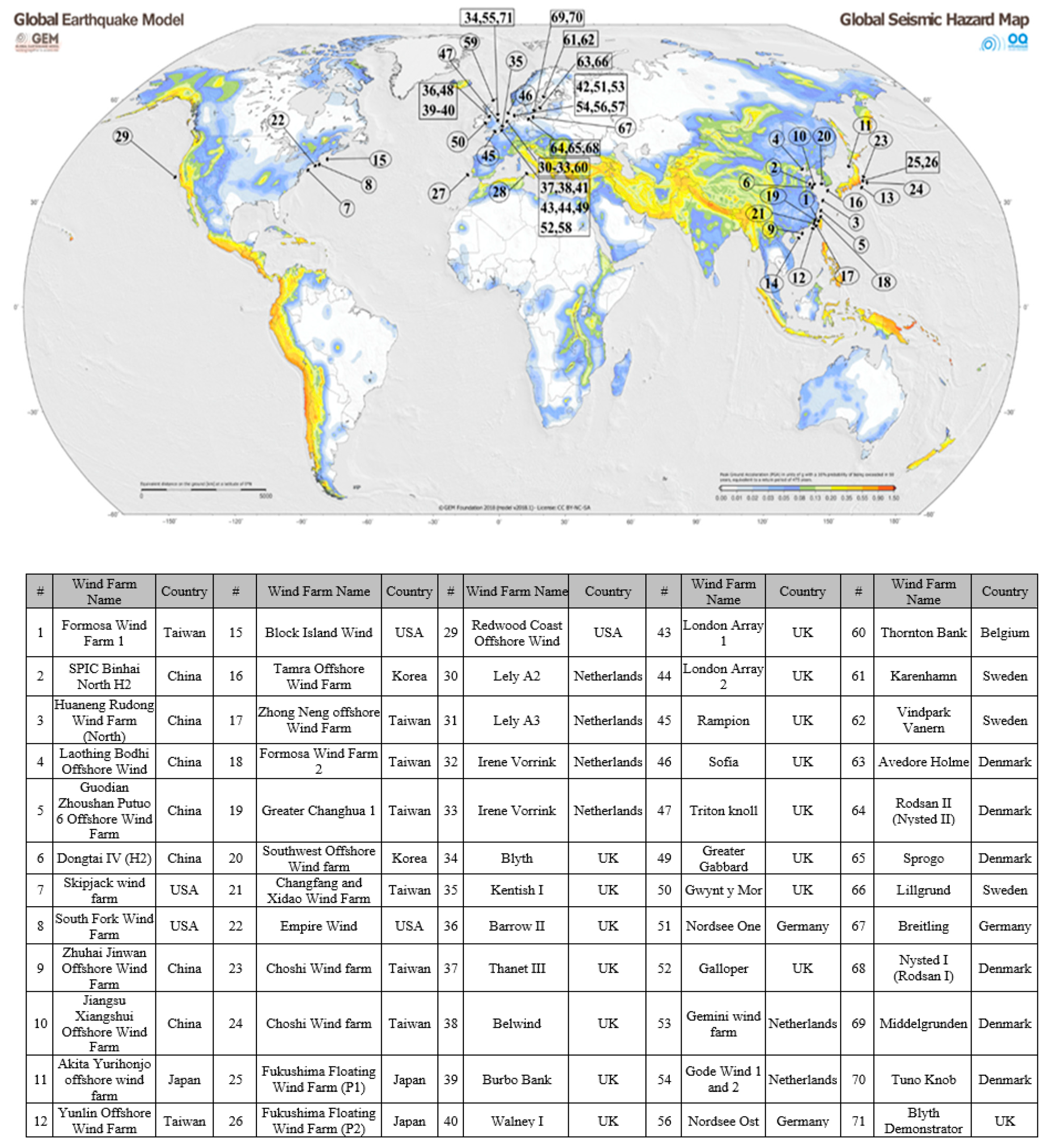
1. Introduction
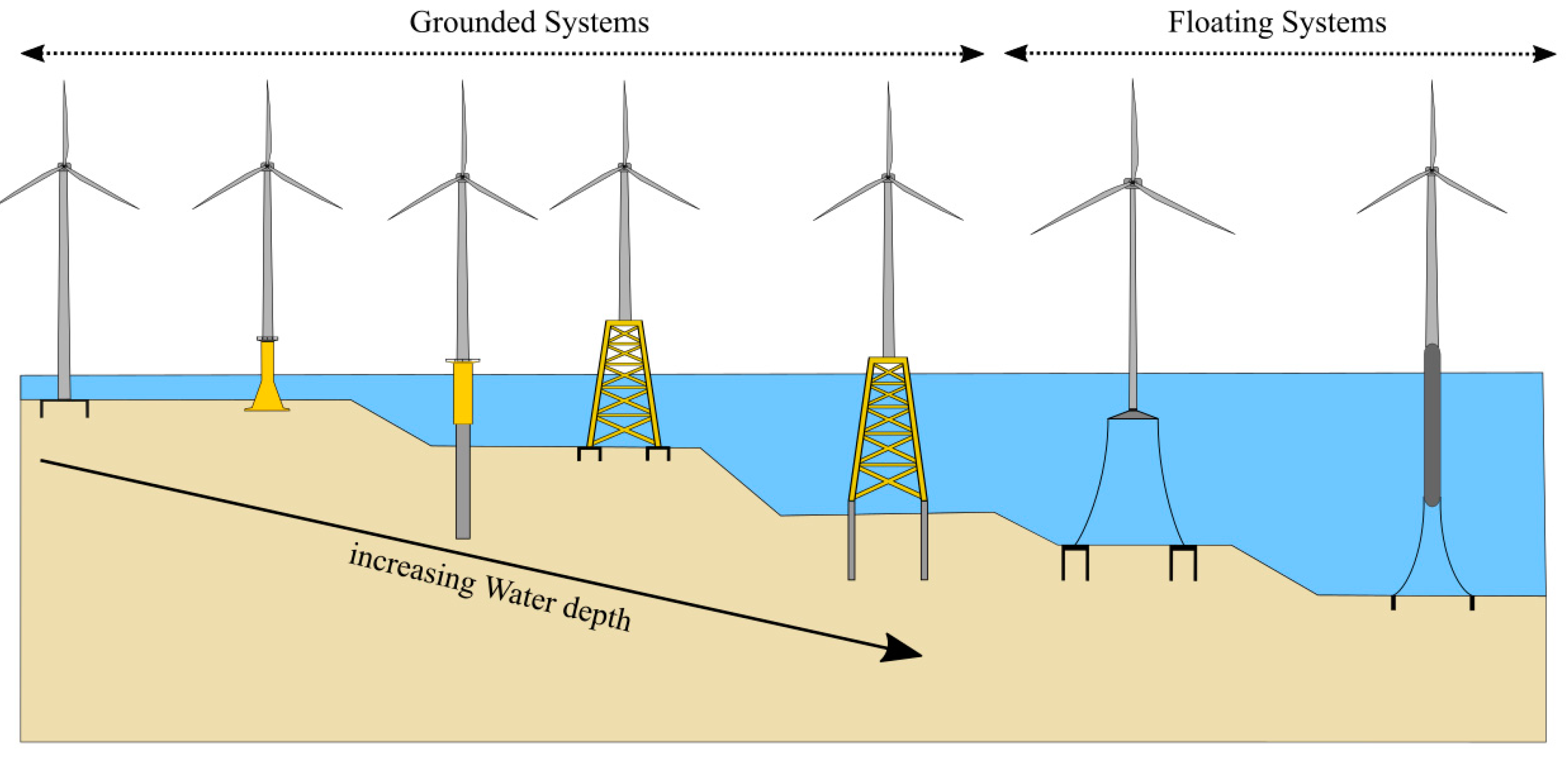
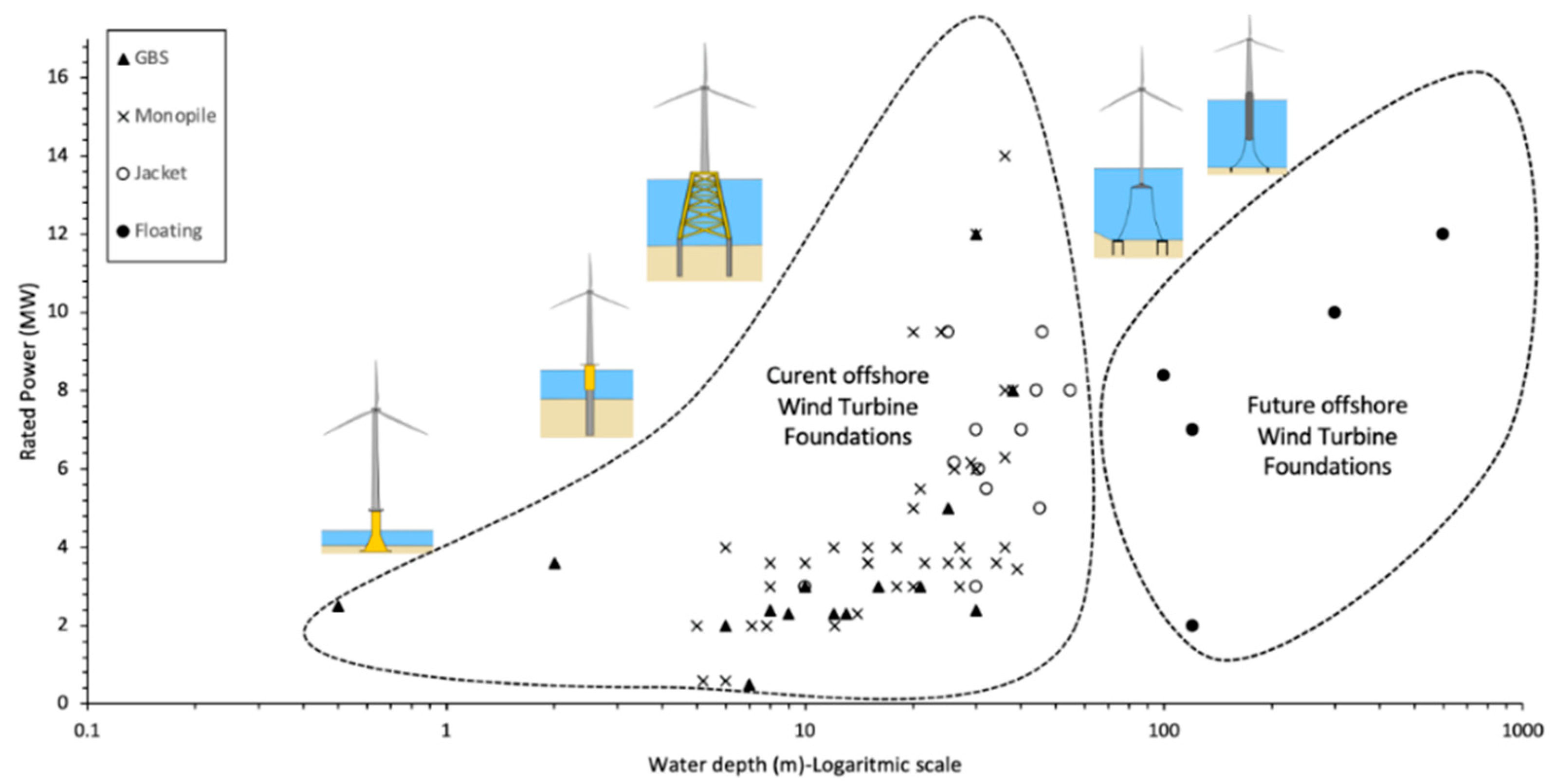
Need for New Types of Foundations
2. Foundations for Offshore Wind Turbines: Complexity in Analysis and Design
- (a)
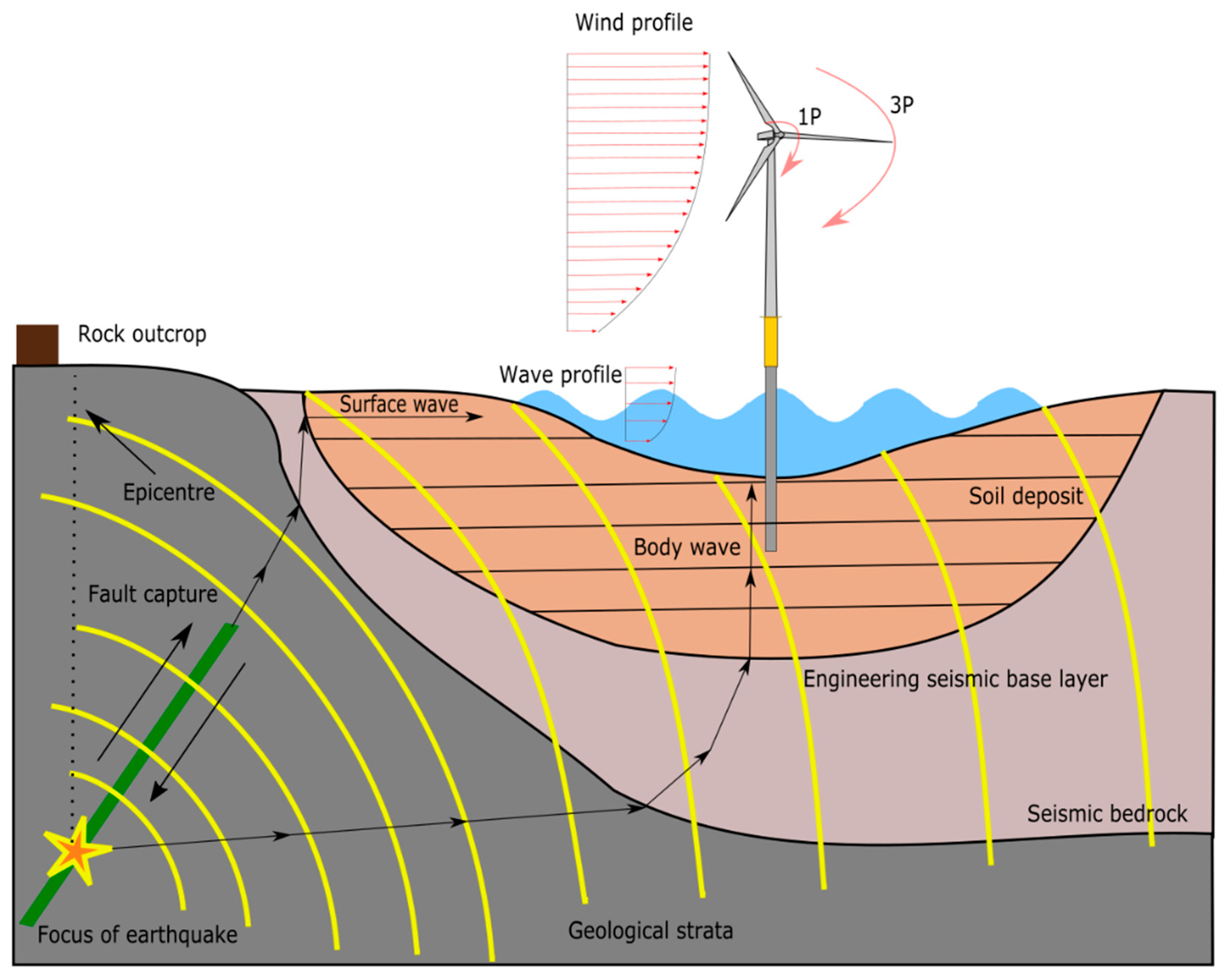
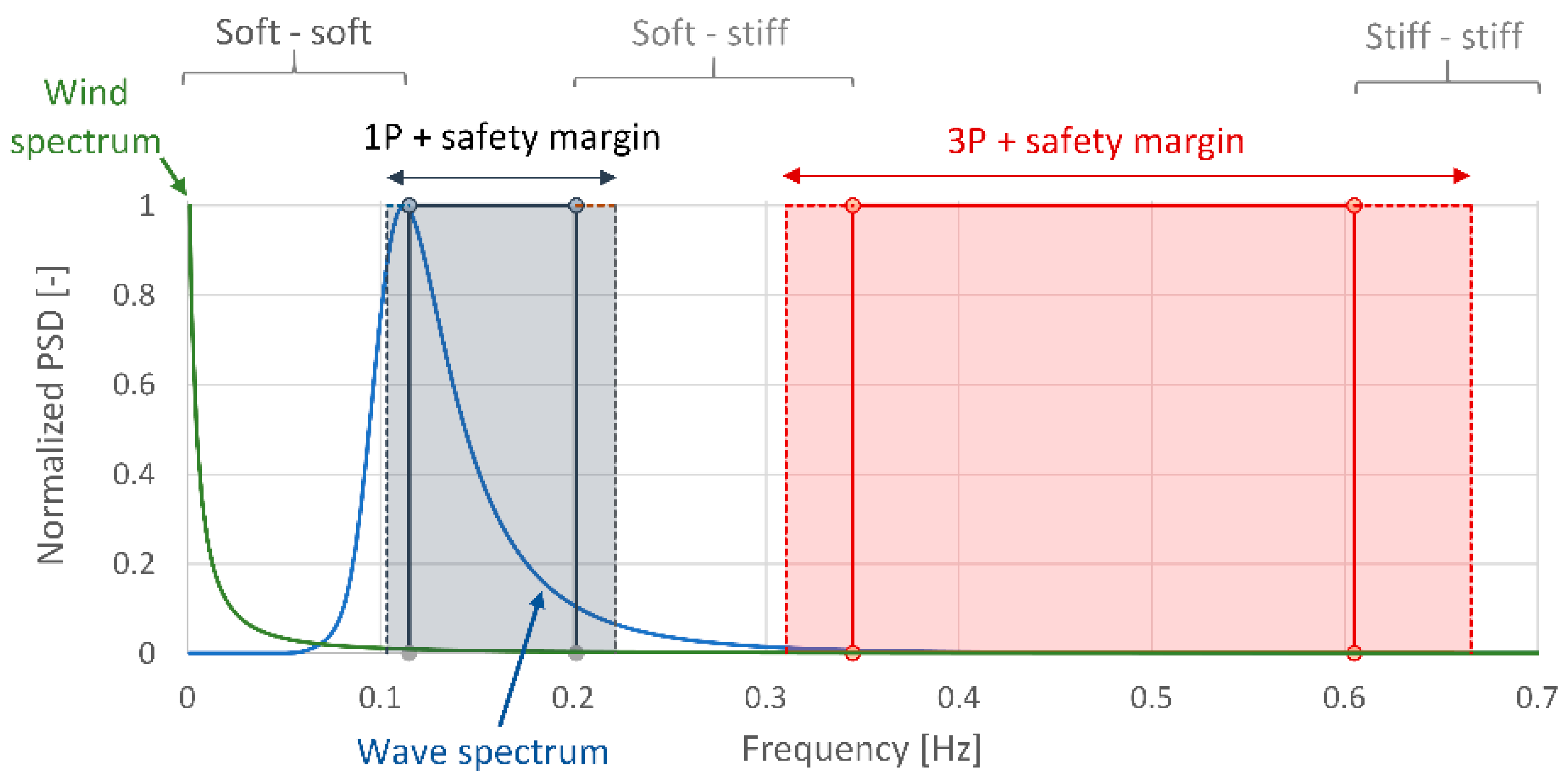
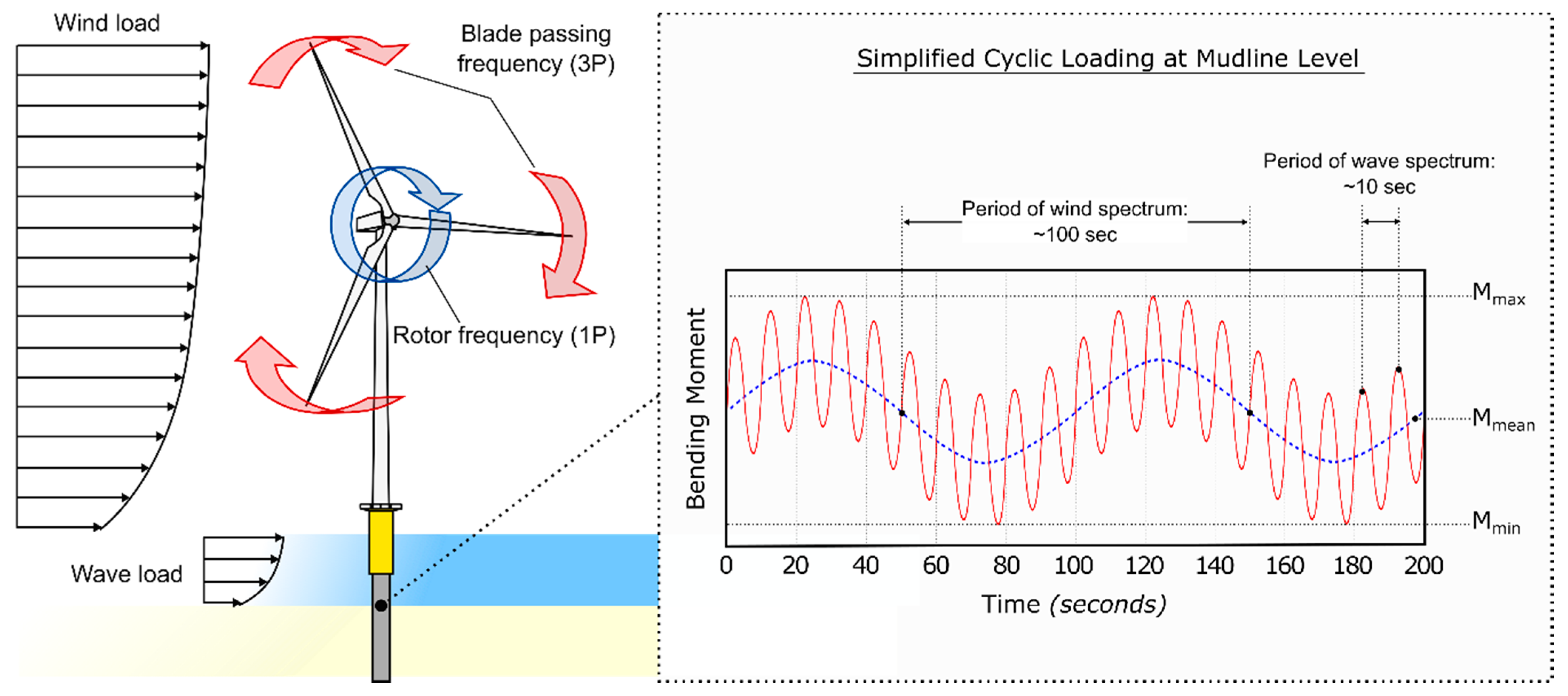
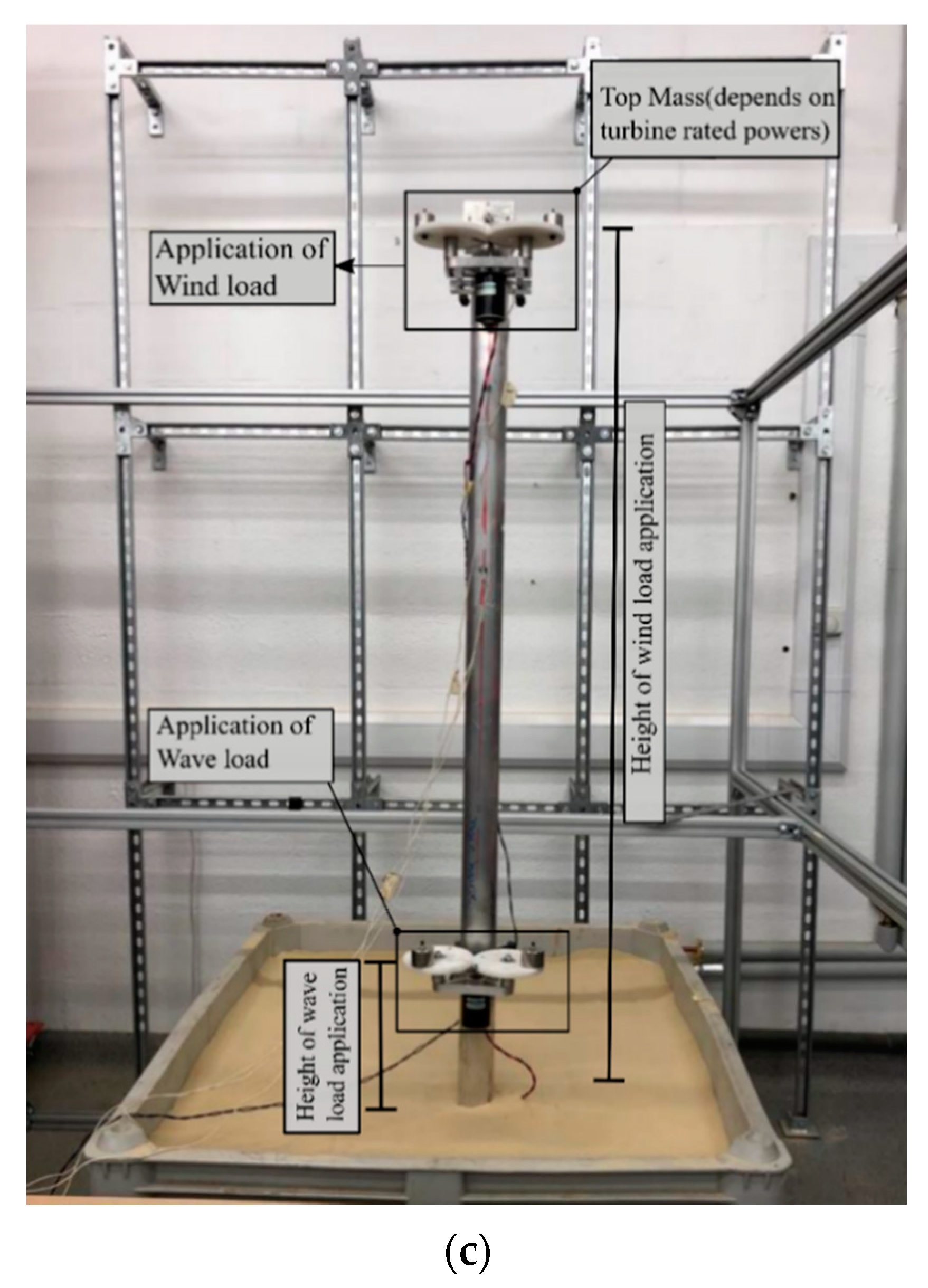
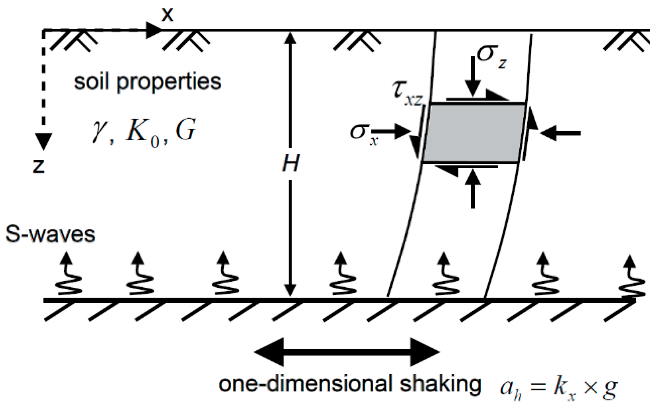
- Wind and wave result in a different offset of amplitude, frequency, and number of cycles applied to the foundation. Figure 8 shows a schematic representation of the frequency of these loads with the frequency intervals corresponding to the three possible design choices: soft–soft, soft–stiff, and stiff–stiff.
- (b)
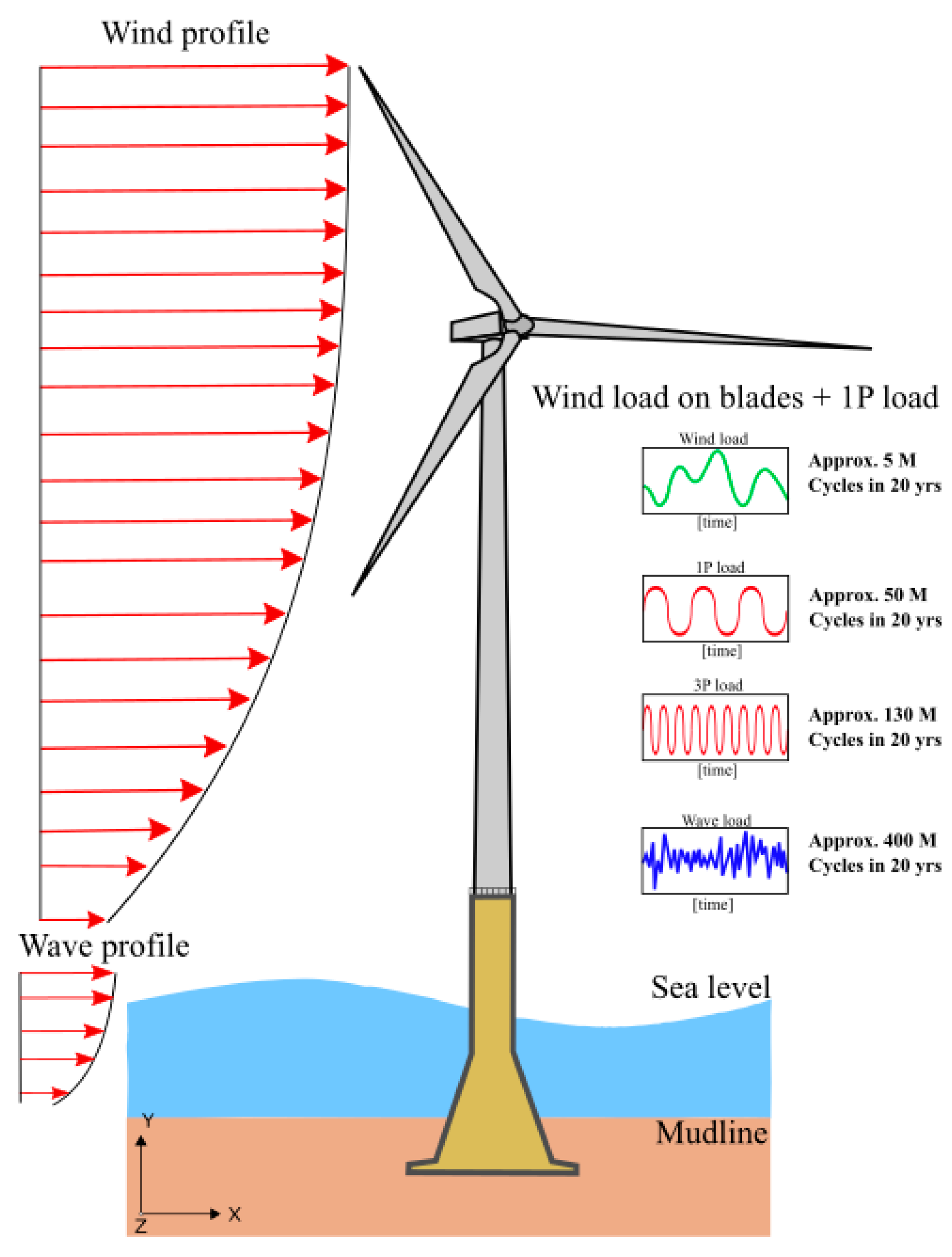
- Wind and the wave loads are random in both space and time, and therefore, they are better described statistically by means of probability distributions, mean values, standard deviation, etc.
- (c)
- Wave and wind load act in two different directions, which give rise to the so-called wind–wave misalignment.
- (d)
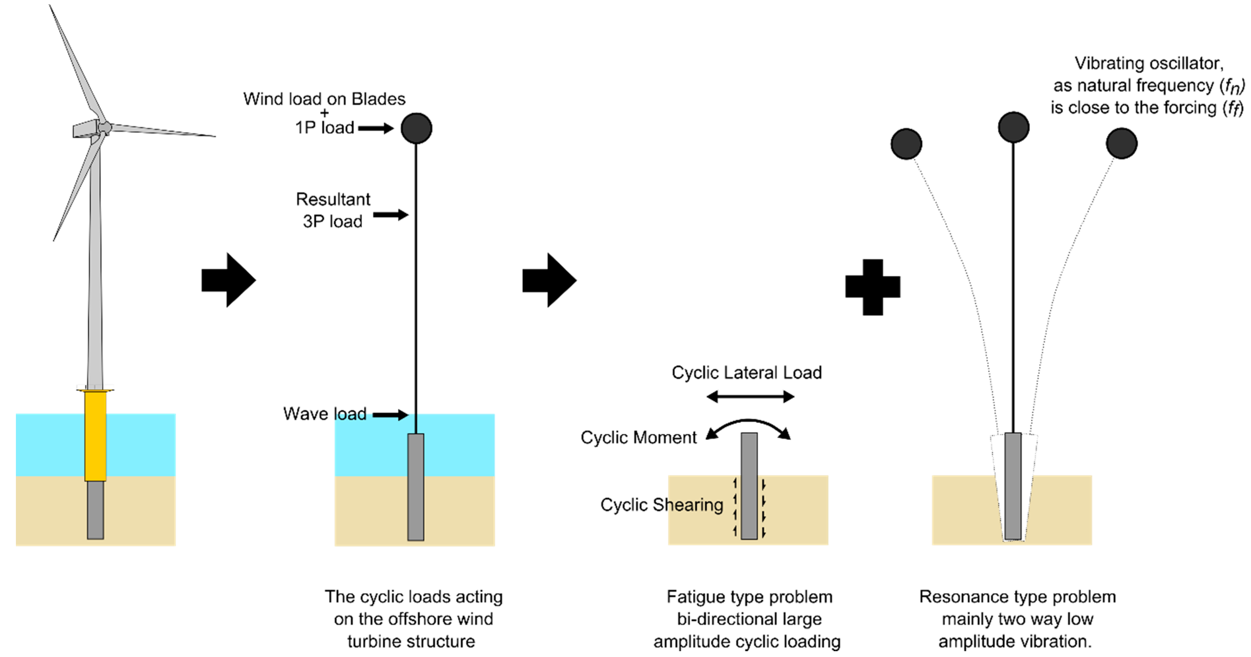
- 1P loading is caused by mass and aerodynamic imbalances of the rotor, and the forcing frequency equals the rotational frequency of the rotor.
- (e)
- 2P/3P loading is caused by the blade shadowing effect, wind shear (i.e., the change in wind speed with height above the ground) and rotational sampling of turbulence. Its frequency is two or three times the 1P frequency for two and three-bladed turbines, respectively. Further details on the loading can be found in [2,3,4,5].
SLS Requirements
- (a)
- The combined pitch and roll should be within 7 to 10 degrees.
- (b)
- The nacelle contains critical components such as gear box, bearings and acceleration that are sensitive to acceleration. The common acceleration adopted for the design is 20% to 30% of g.
- (c)
- Translational displacement, also referred to as excursion, which needs to be kept within 20% of water depth.
- (a)
- Possible liquefaction of loose to medium-dense sand deposits, which may induce permanent tilting to bottom-fixed foundations or loss of uplift capacity to anchors of floating systems.
- (b)
- Excessive vibrations due to resonance effects when the predominant frequency of the earthquake comes close to one of the fundamental frequencies of the structure.
3. Physical Modelling in Geotechnical Engineering: A Brief Overview
- To verify the analysis/design methodologies of high-risk or novel construction techniques. For example, suction caissons are being used in North Sea grounds comprising dense sands or firm clay, and it is necessary to verify if a similar technique can be used in Chinese sites with soft soil condition. A second example is to evaluate the applicability of pressure reversal (often known as pressure cycling) to install suction caisson foundations and its effect on the post-installation uplift capacity.
- To recreate a failure or a collapse mechanism for settling liabilities or insurance claims.
- To gain new insights into unexplored complex phenomena that cannot be investigated in the real field or modelled in numerical simulations due to the lack of adequately accurate soil constitutive equations. An example may include tests to investigate the cyclic behaviour of foundations in shallow gassy sediments.
- To verify different aspects of the design for a new concept of a foundation type for which no codes of practice/guidelines or prior experience exist; that is, reducing the uncertainties in the design assumptions. Examples of particular design aspects for this specific problem of a new foundation can be modes of vibration or the modes of ultimate collapse.
- To understand the deformations of foundations under various design situations and limit states
- To develop design methods that may lead to the path of standardization and to validate the constitutive models of soils used in numerical models.
4. Physical Modelling of Offshore Wind Turbine Foundations
4.1. Requirements of Foundation Testing for Offshore Wind Turbine Foundations
- (i)
- Load transfer from the superstructure to the supporting ground in the case of extreme load events.
- (ii)
- Modes of vibration of the adopted structural system, i.e., rigid rocking modes or flexible modes or a combination.
- (iii)
- Long-term change in dynamic characteristics, i.e., change in natural frequency and damping due to repetitive cyclic loads or extreme dynamic loads associated with natural hazards such as typhoons and earthquakes.
- (iv)
- Long-term deformation does not violate stringent SLS requirements, such as being limited to maximum rotation.
4.2. Suitability on Different Methods of Testing
- (a)
- Wind tunnel testing can model the aerodynamics and aeroelasticity interaction, and the performance of the blades.
- (b)
- Wave tanks can be used to model hydrodynamic issues, including tsunami loads.
- (c)
- Geotechnical centrifuge testing can model soil–structure interactions with correct stress–strain behaviors.
- (d)
- A shaking table at 1 g or in a geotechnical centrifuge can model the seismic performance, including dynamic soil–structure interaction (DSSI).
4.3. STEPS in Designing Scaled Mode Tests
- (a)
- List all of the failure mechanisms (however improbable they are) and then rank them. Write down the governing equations based on simple mathematical idealization. In this context, readers are referred to the work of Adhikari and Bhattacharya [23,27] on the non-dimensionalization of the Euler–Bernoulli equation considering the flexibility of the foundation.
- (b)
- Carry out finite element analysis of the same problem as a sanity check because not all of the parameters can be accounted for in the simple idealistic analysis.
- (c)
- Following the above two steps, scaling and derivation of the similitude relationships can be undertaken. Then, the experiments can be designed and carried out.
- (d)
- Verify if the experiments show the predicted behavior. Subsequent rounds of experimentation may be required depending on the outcome. New lessons may be learnt that were previously thought to be unimportant, and vice versa.
- (e)
- Iterate the above procedure until the convergence of understanding.
- DO
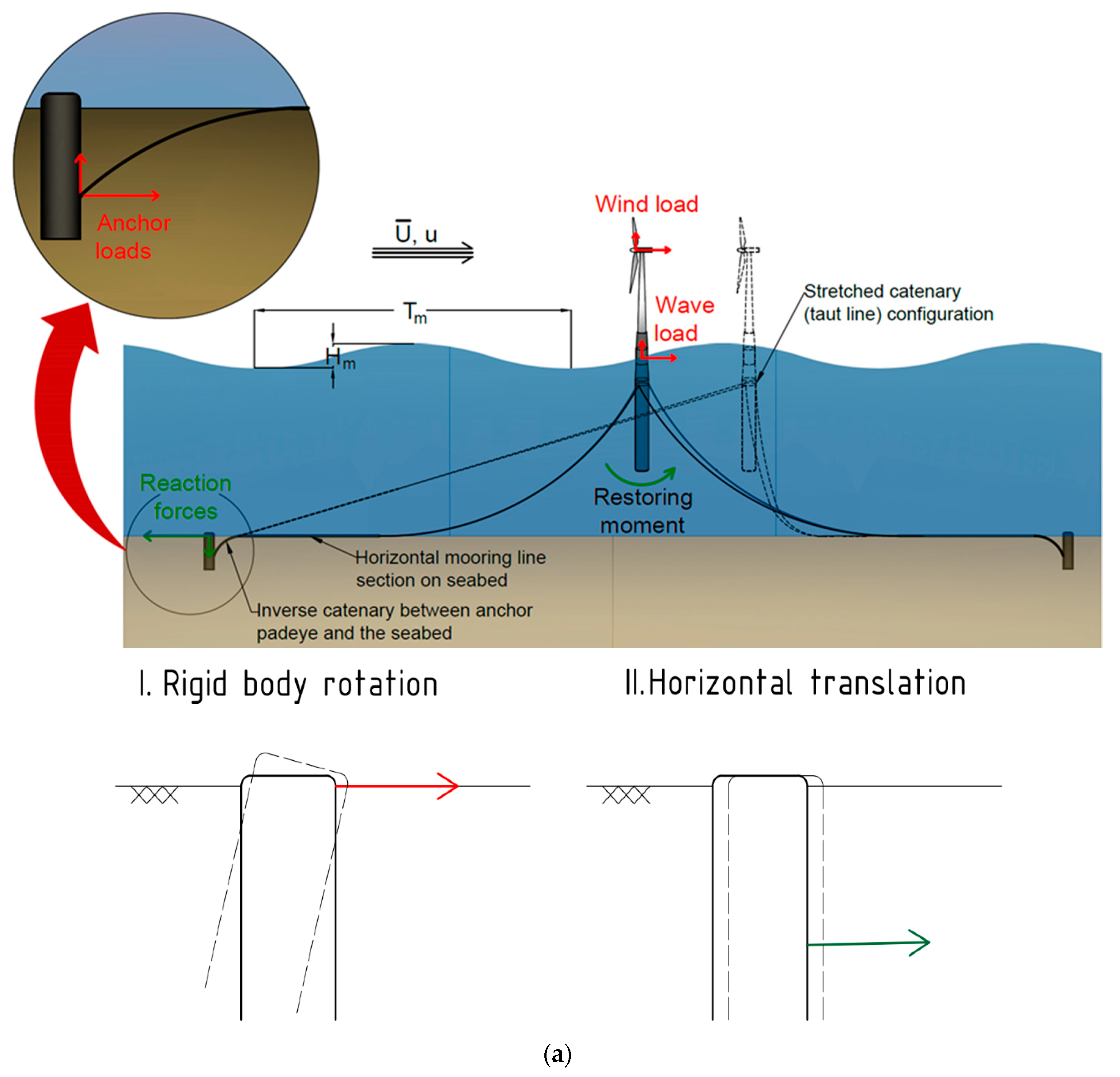
- It is important to replicate the mechanisms (for example, failure mechanism) in small-scale tests. This is shown below using the example of the failure of an anchor foundation for floating wind turbines, i.e., the verification of Ultimate Limit State (ULS) design.
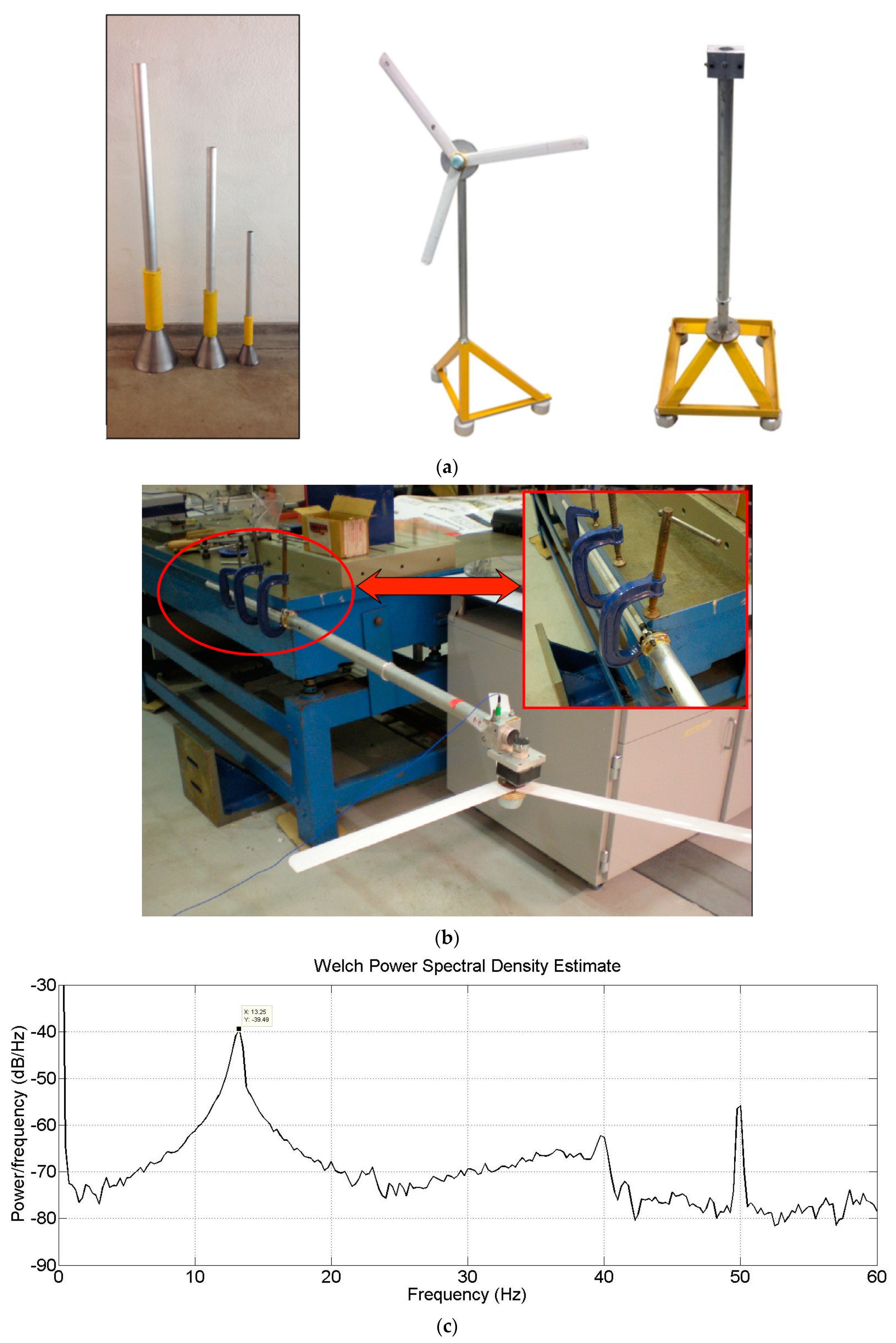
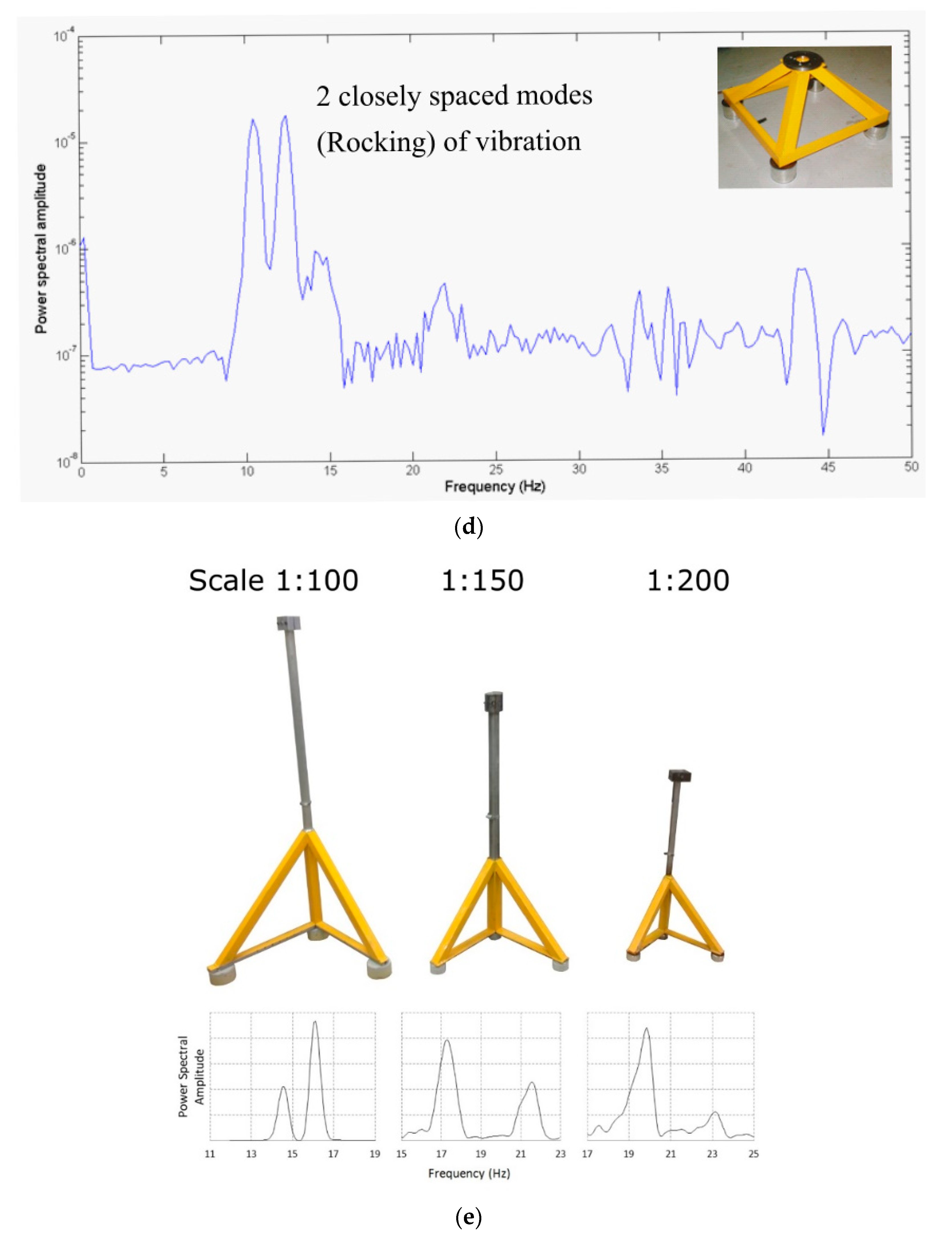
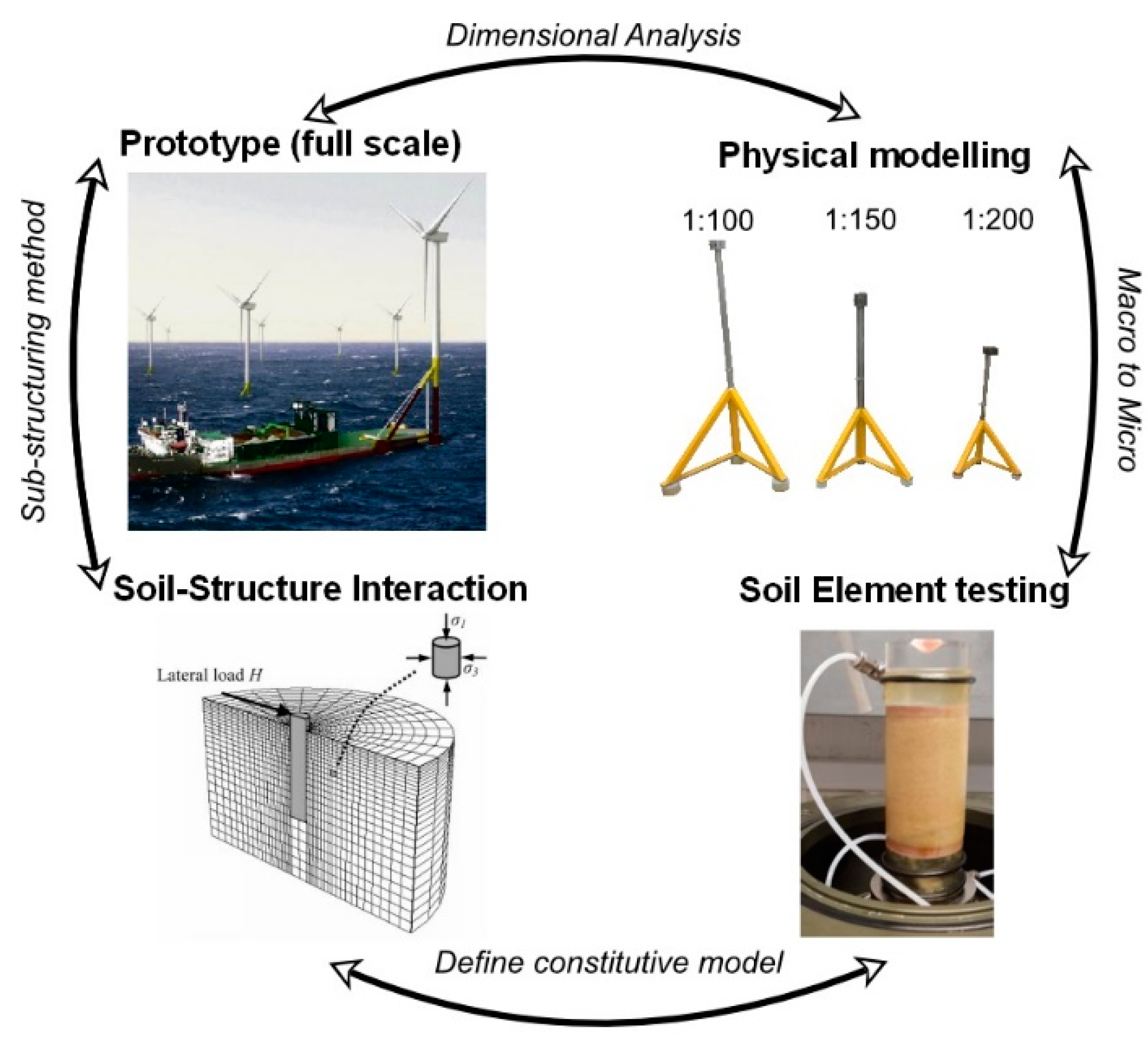
- Each test needs to be repeated at several scales (at least three), such as 1:200, 1:100, and 1:50. This is often termed “Modelling of models” in the literature to remove artefacts (if any) and to establish reliability. Nonlinearity is defined by amplitude, and this step helps to identify non-linear behaviour. It is shown below that two peak modes of vibration were identified for turbines supported on multiple shallow foundations.
- Physical mechanisms or processes (essentially the laws of physics) must be identified that govern the observation or control the behavior of interest. This can guide Serviceability Limit State (SLS).
- If possible, the governing equation should be written and, using mathematical techniques, the non-dimensional groups should be identified.
- Check nonlinearity of the non-dimensional groups.
- DO NOT
- Unless it is a very simple problem, do not scale the numerical values of the observations to predict the prototype consequences. There is often a tendency to use standard charts and scale the observations.
5. Mechanisms to Be Considered in Scaled Modelling for Offshore Wind Turbine Foundations
- (a)
- Confirmation and validation of the mechanism of load transfer from the superstructure to the ground through the foundation element. This is very important for a new concept of a foundation or a connection. For example, adding a circular plate around a pile may increase the bearing capacity and improve resistance to overturning. Although this is a conjecture, and it must be verified through testing. Furthermore, the long-term effects of the foundation under scour or cyclic loading must be verified.
- (b)
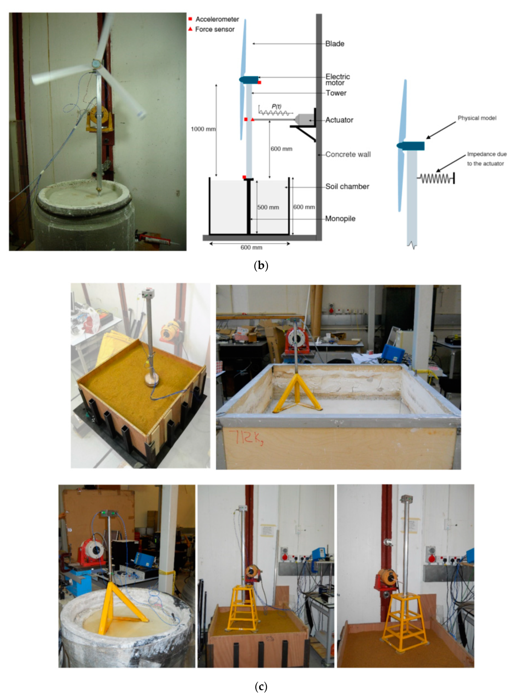
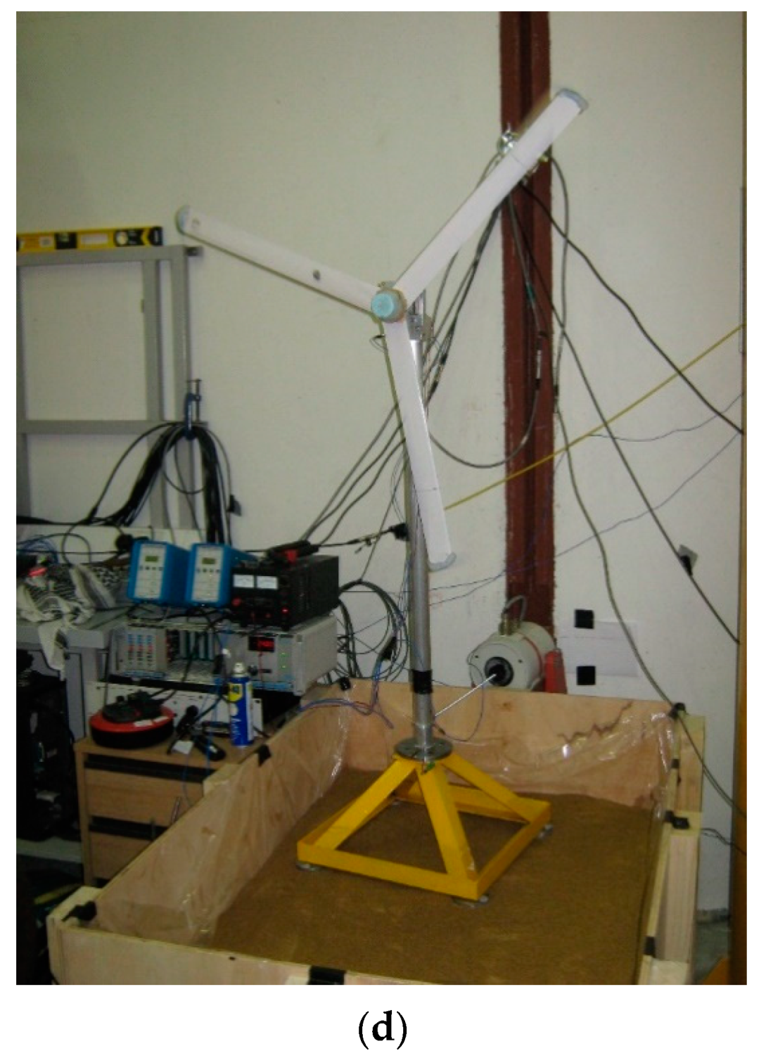
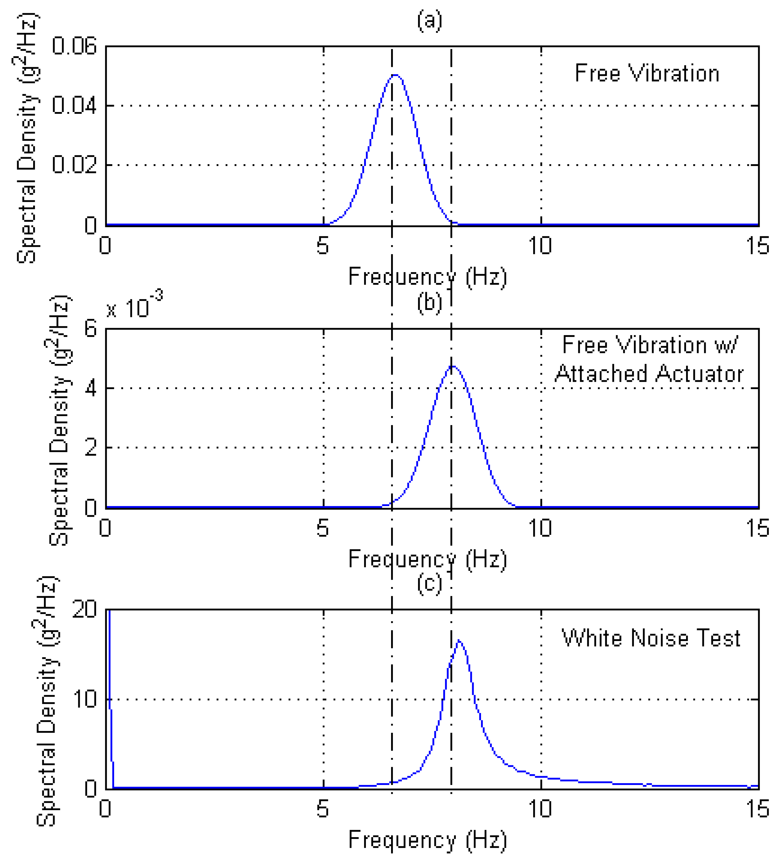
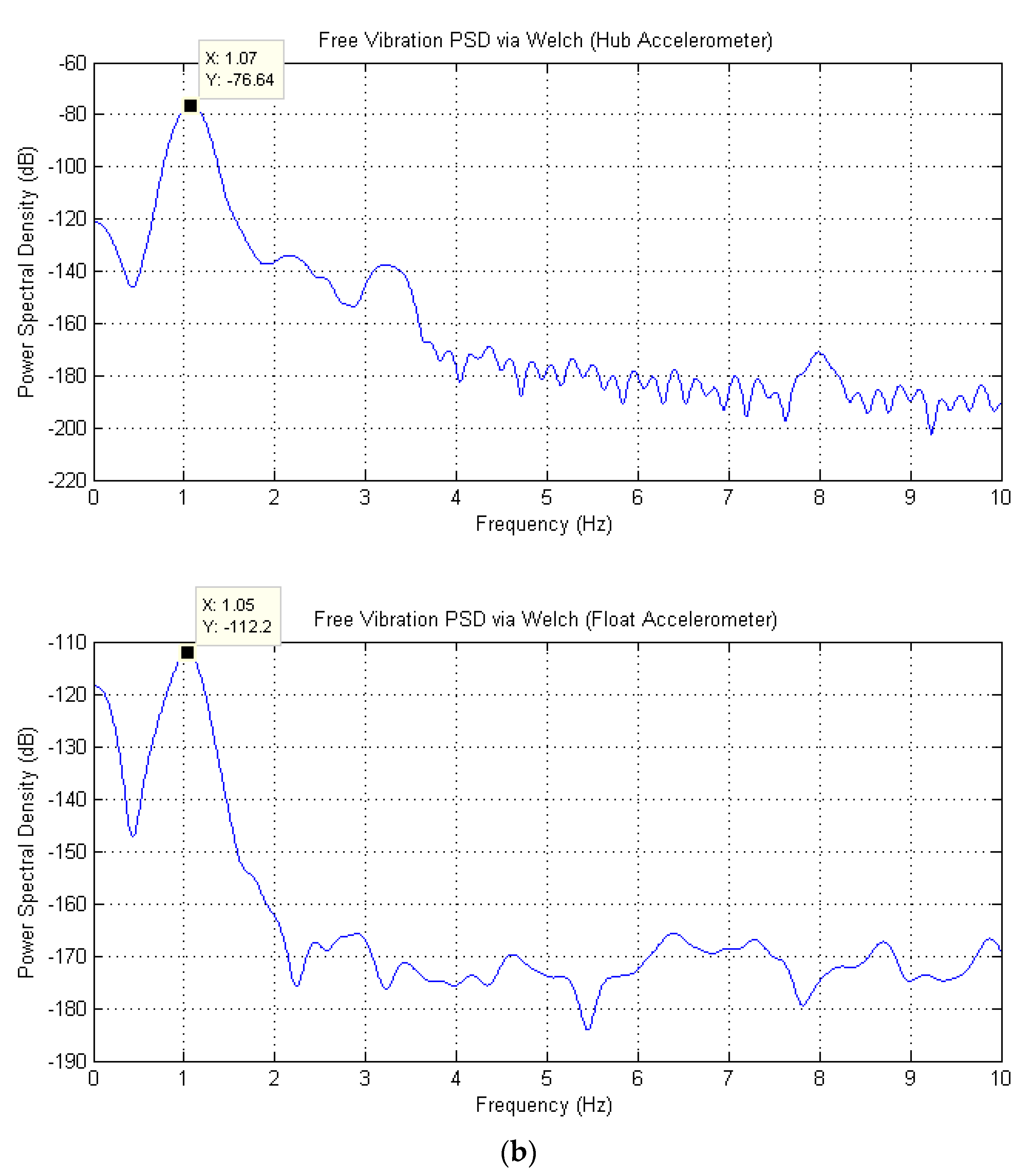
- Because offshore wind turbines are dynamically sensitive structures, modes of vibration of the structures are very important. These can be carried out through free vibration/perturbation tests or white noise testing. This is an important part of the validation process because modes of vibration can strongly influence the foundation design, fatigue life, and wear and tear of the mechanical components in the RNA.
- (c)
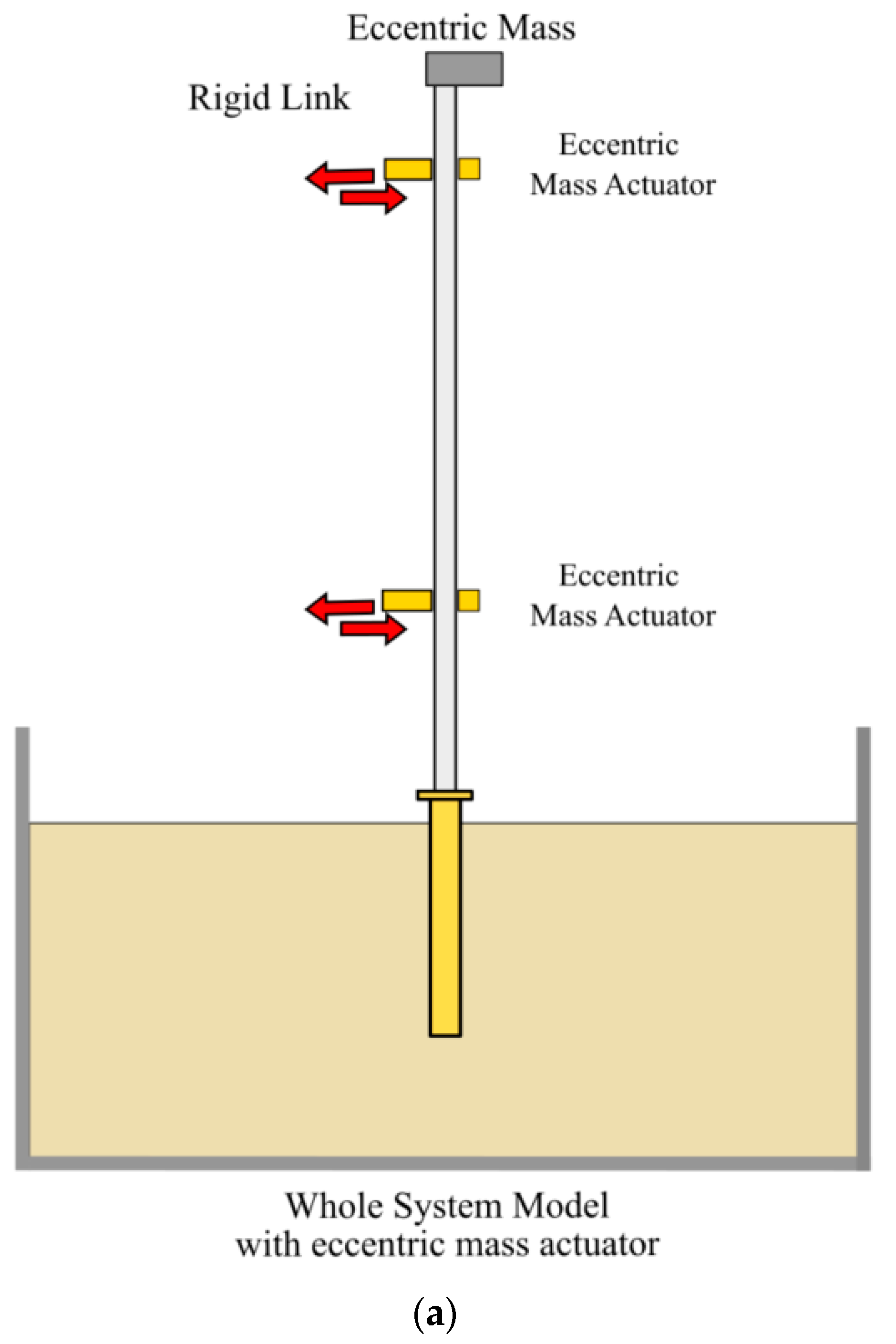
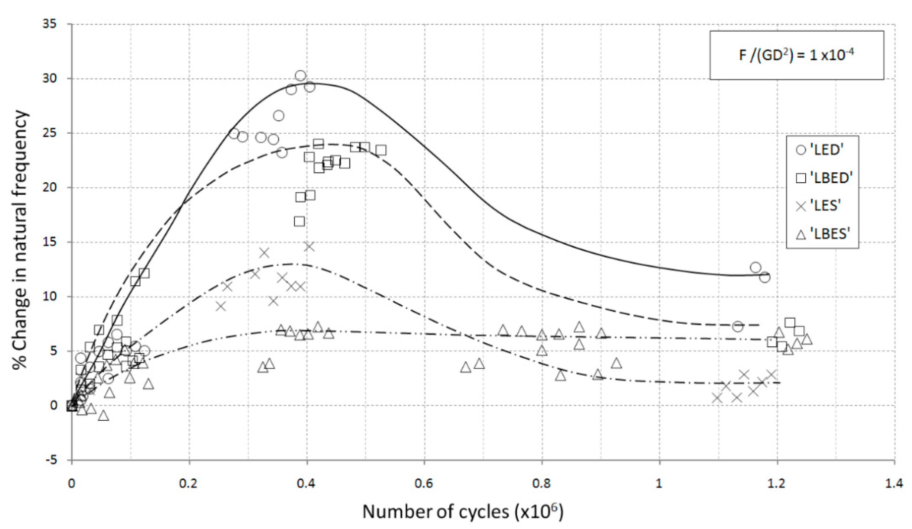
- Foundations for offshore wind turbines are subjected to hundreds of millions of loading cycles, which can be cyclic or dynamic in nature. Scaled model tests can reveal the expected trends of the behaviour of the foundations due to cyclic and dynamic soil–structure interaction. One of the uncertainties is the long-term non-recoverable tilt of the foundation. Excessive tilt may lead to shut down of the turbine due to loss of warranty.
- (d)
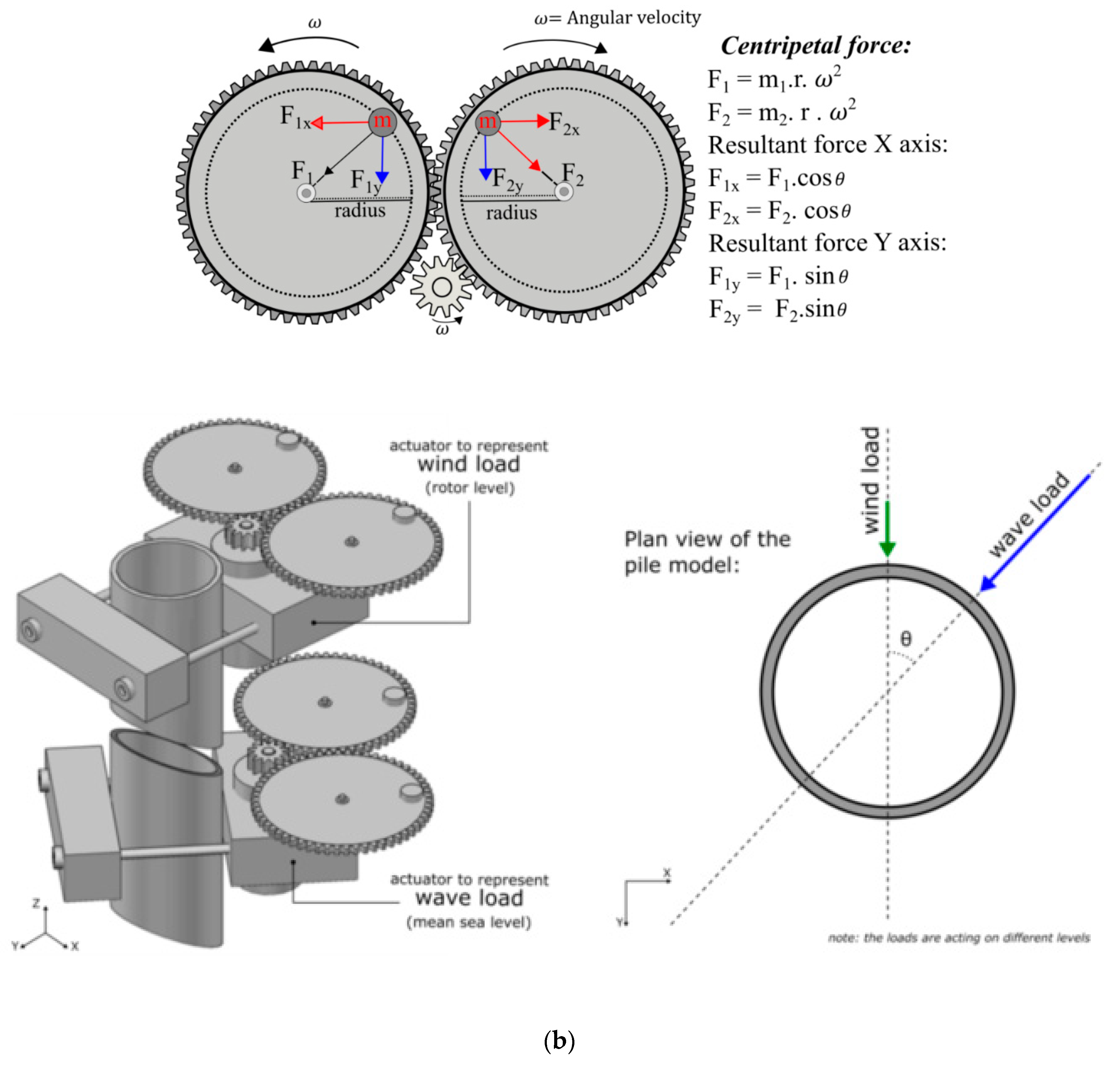
- The environmental loads transferred to the foundation of offshore wind turbines are very complex; they can be simplified as one-way cyclic or two-cyclic waveforms. The long-term effects of such waveforms can be identified through scaled model tests.
- (e)
- Due to dynamic sensitivity, offshore wind turbines need damping. Trends and sources of damping can be identified through carefully designed scale model tests.
5.1. Types of Scaled Model Apparatus
5.2. Measurement of Dynamic Response and Type 2 Technique
White Noise Testing
5.3. One the Use of “Reductionist” Approach [Type 1 versus Type 3] for Grounded System
6. Example of Scaled Model Tests
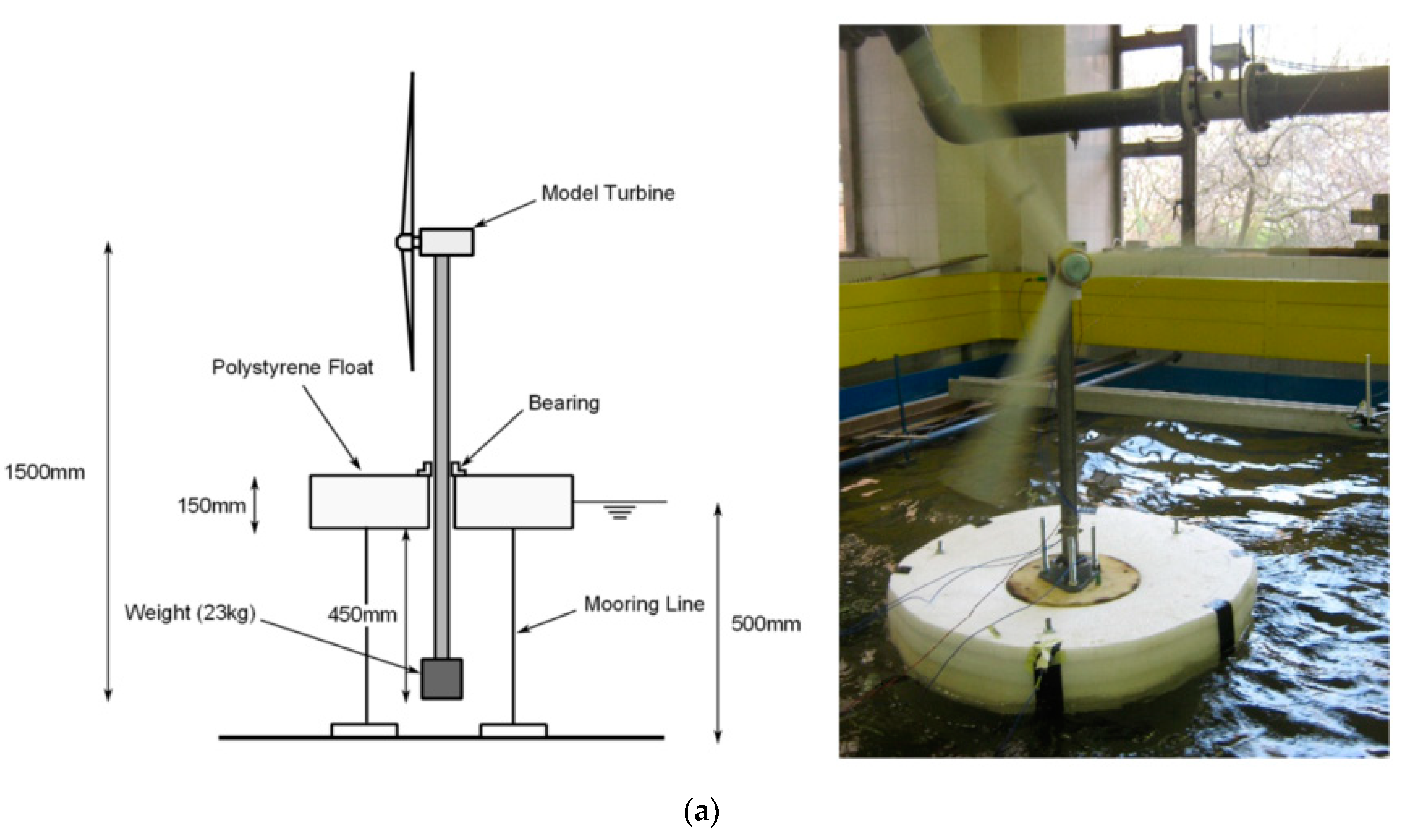
6.1. Proof of Concept of Floating Systems
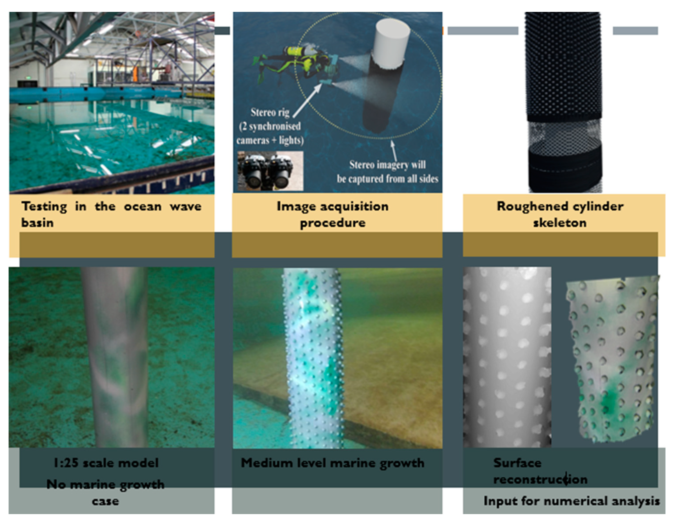
6.2. Example of Scaled Test on Biofouling on Monopiles
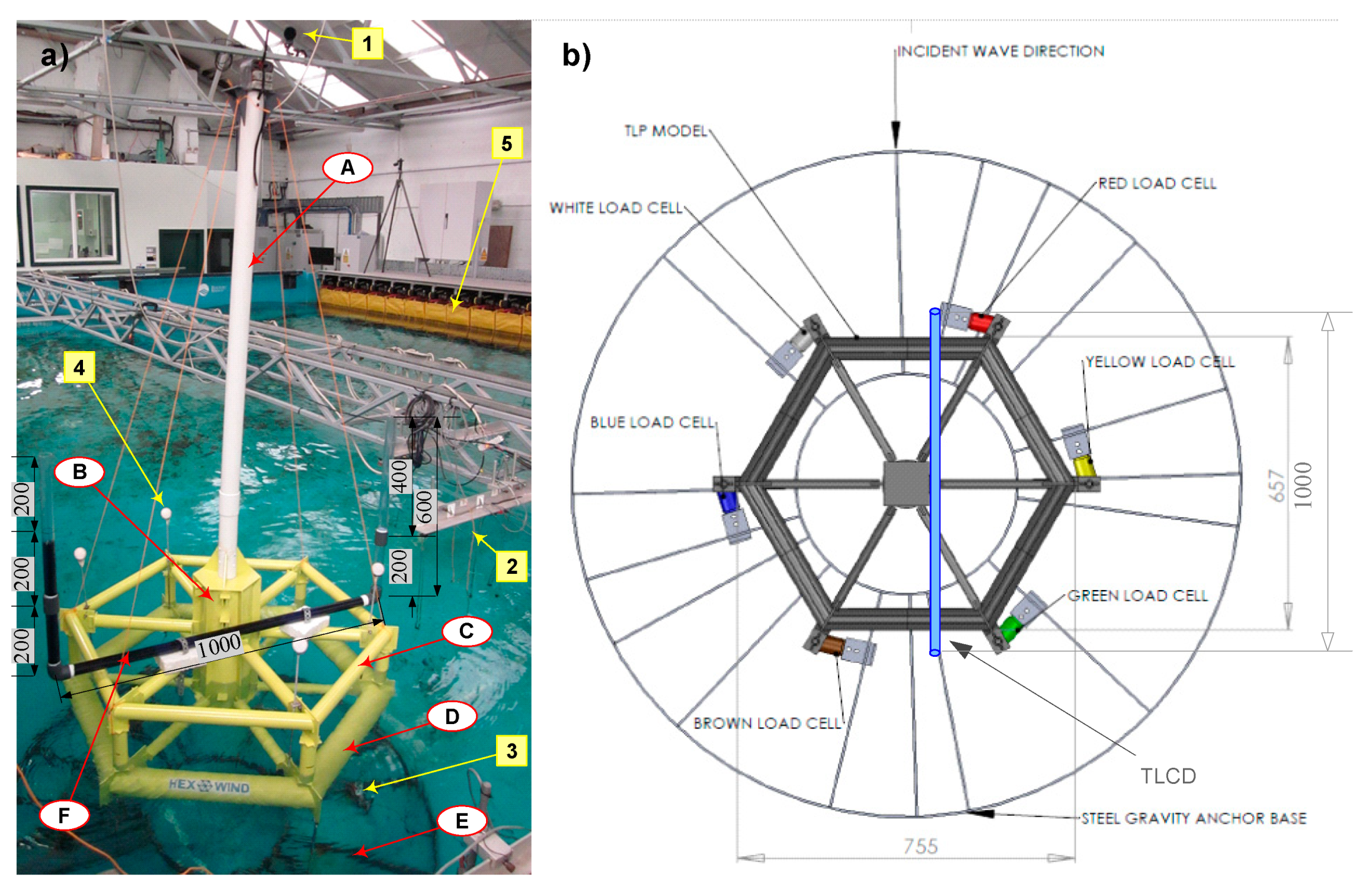
6.3. TLP Experiment
6.4. Verification of Failure Modes of Anchor Foundations for Spar Type
6.5. Modes of Vibration of Systems
- (a)
- Mass similarities, i.e., mass distribution along the length of the tower;
- (b)
- Stiffness similarity, i.e., relative tower to foundation similarity;
- (c)
- Geometric similarity, i.e., the relative distance between the foundation in proportion to the tower must be preserved.
- (a)
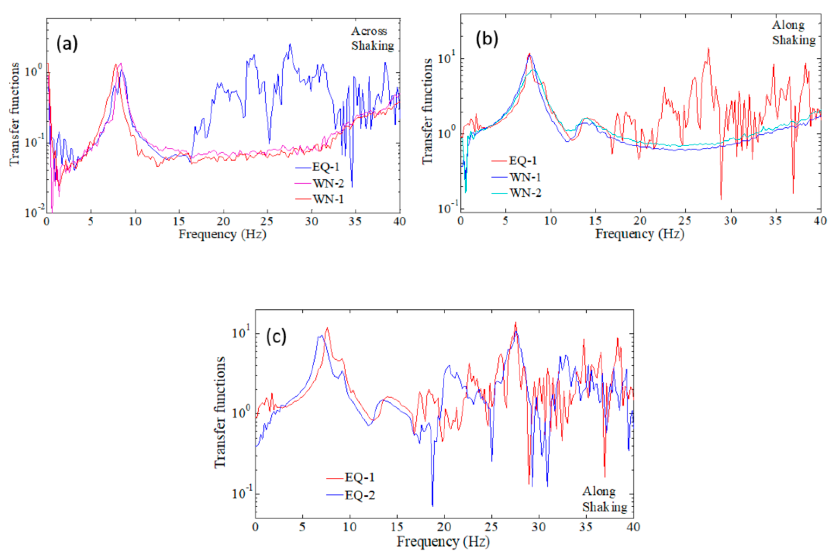
- Sway-bending, i.e., flexible modes of the tower without rocking modes of foundations. This is typical of any wind turbine systems on deep foundations. Figure 23c shows an example of a twisted jacket on pile foundations where the first mode is distinct from the second mode.
- (b)
- Rocking mode of vibration, which occurs due to the rigid rocking of foundations and will be manifested with two closely spaced modes. Figure 23d,e shows two examples. For the symmetric arrangement of foundations (i.e., tetrapod), the initially observed closely spaced peaks will merge into a single peak after tens of thousands of cycles. However, for asymmetric systems (i.e., the system shown in Figure 23e), these peaks converge.
6.6. Centrifuge Modelling
6.7. Earthquake Response of Wind Turbine Structures
7. Scaling the Test Results
- Example 1: Physical Modelling of asymmetric foundations.
- Example 2: Physical modelling for the seismic design of piled foundations in liquefiable soils
- (a)
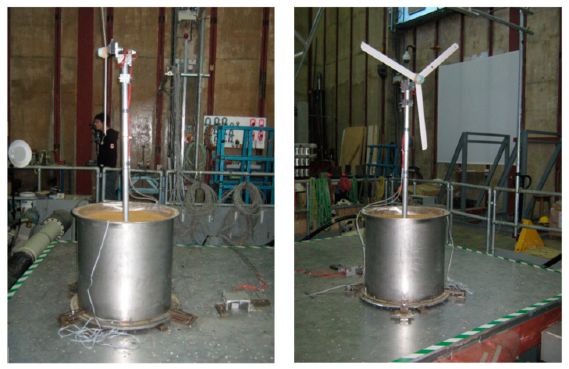
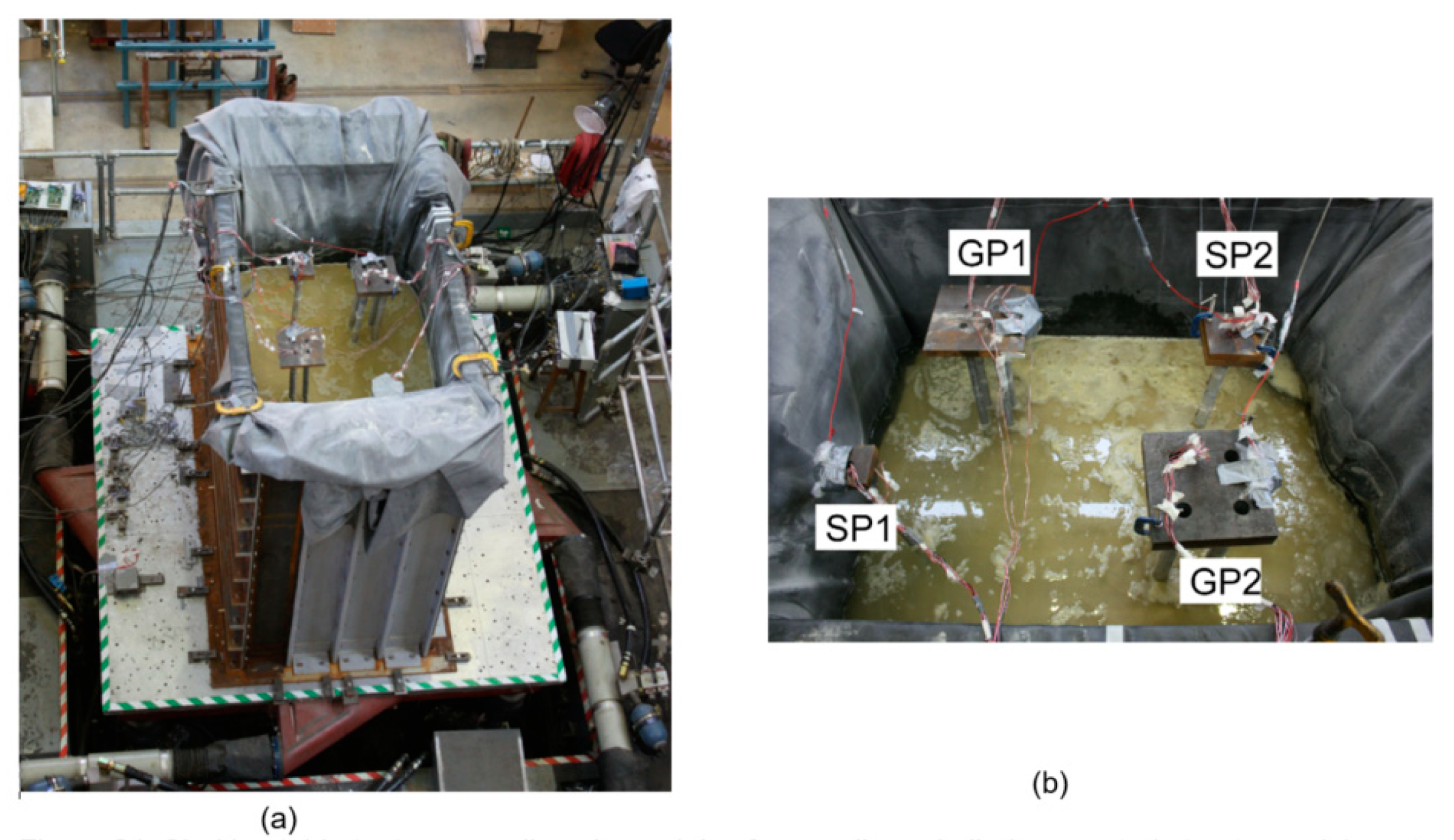
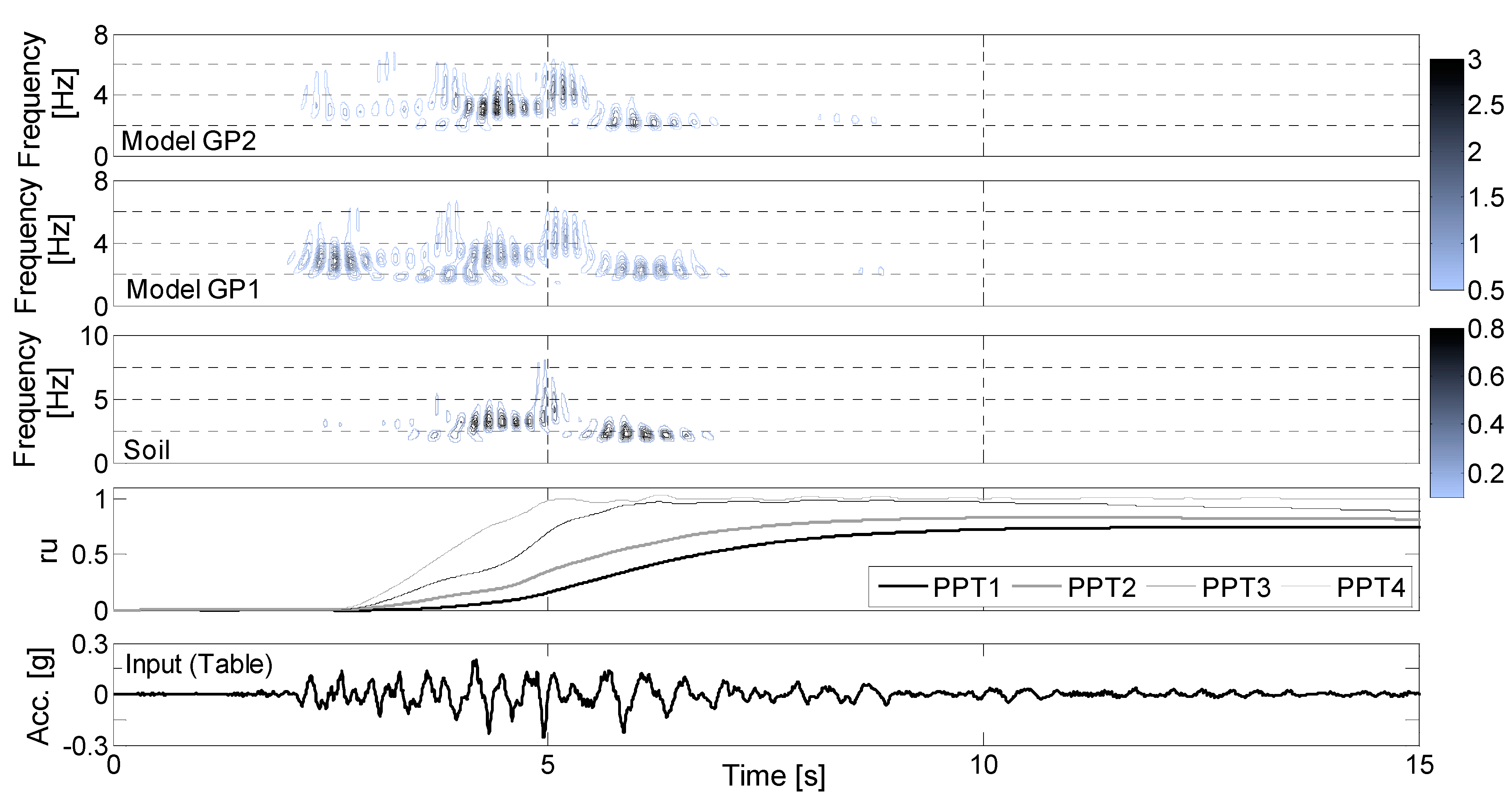
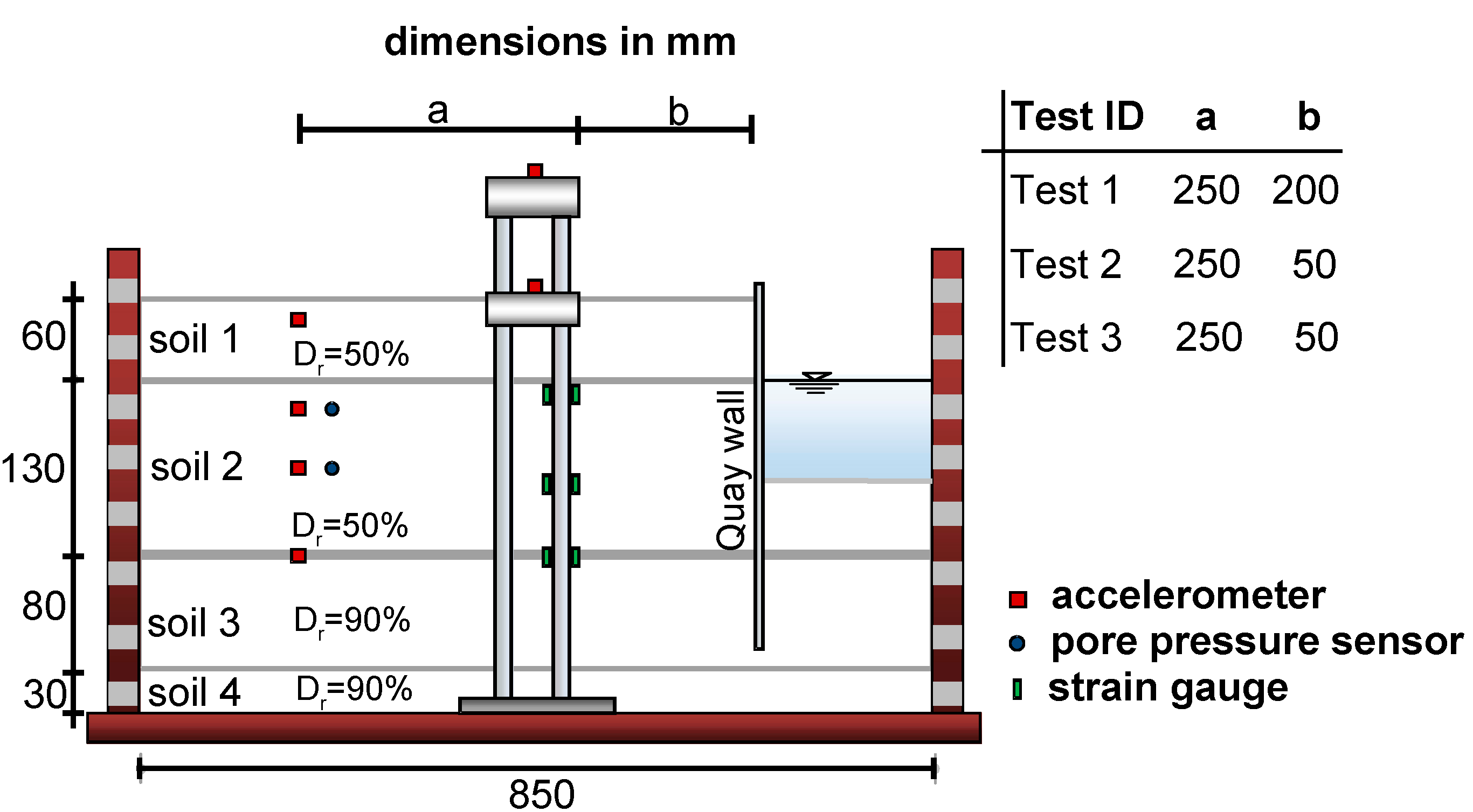
- The understanding of pile–liquefied soil interaction was understood from both shaking table tests (see Figure 31 for the setup at 1–g) and centrifuge tests. In both experiments, results showed that the liquefied soil offers negligible support to a vibrating pile and the damping of the whole system increases when the soil is liquefied.
- (b)
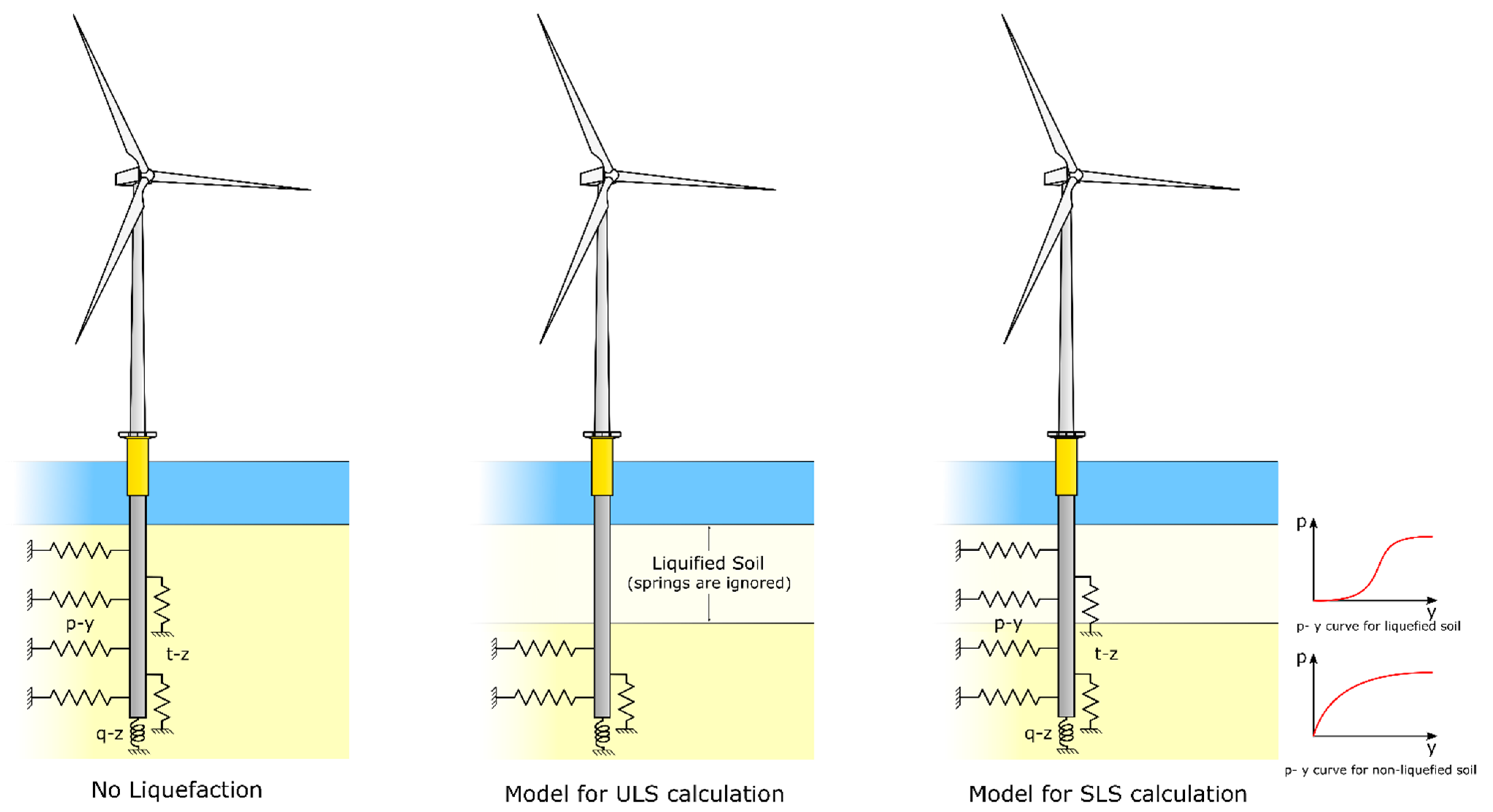
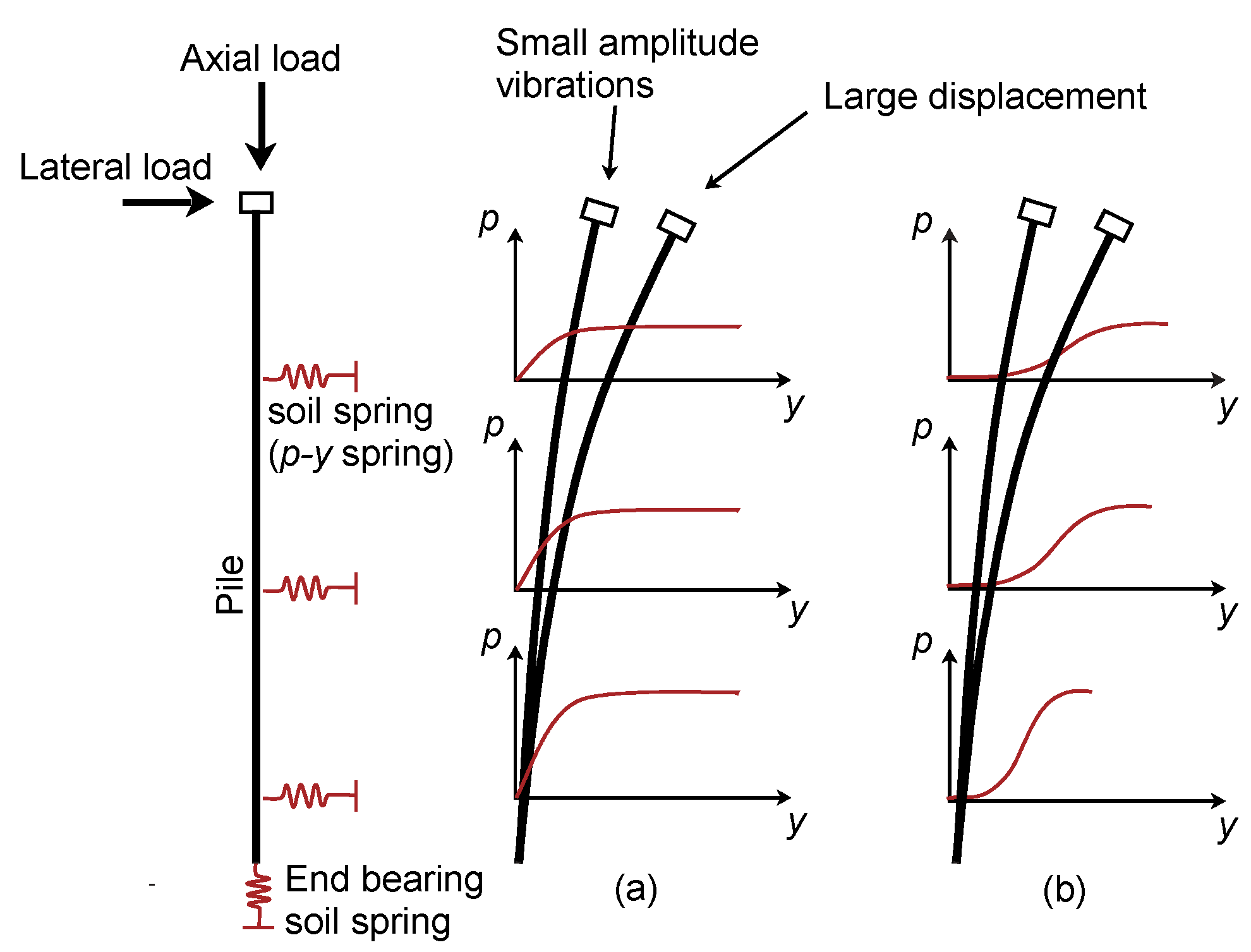
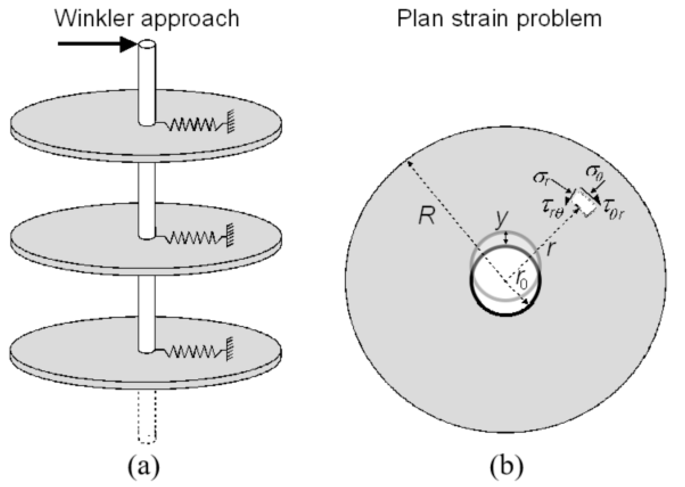
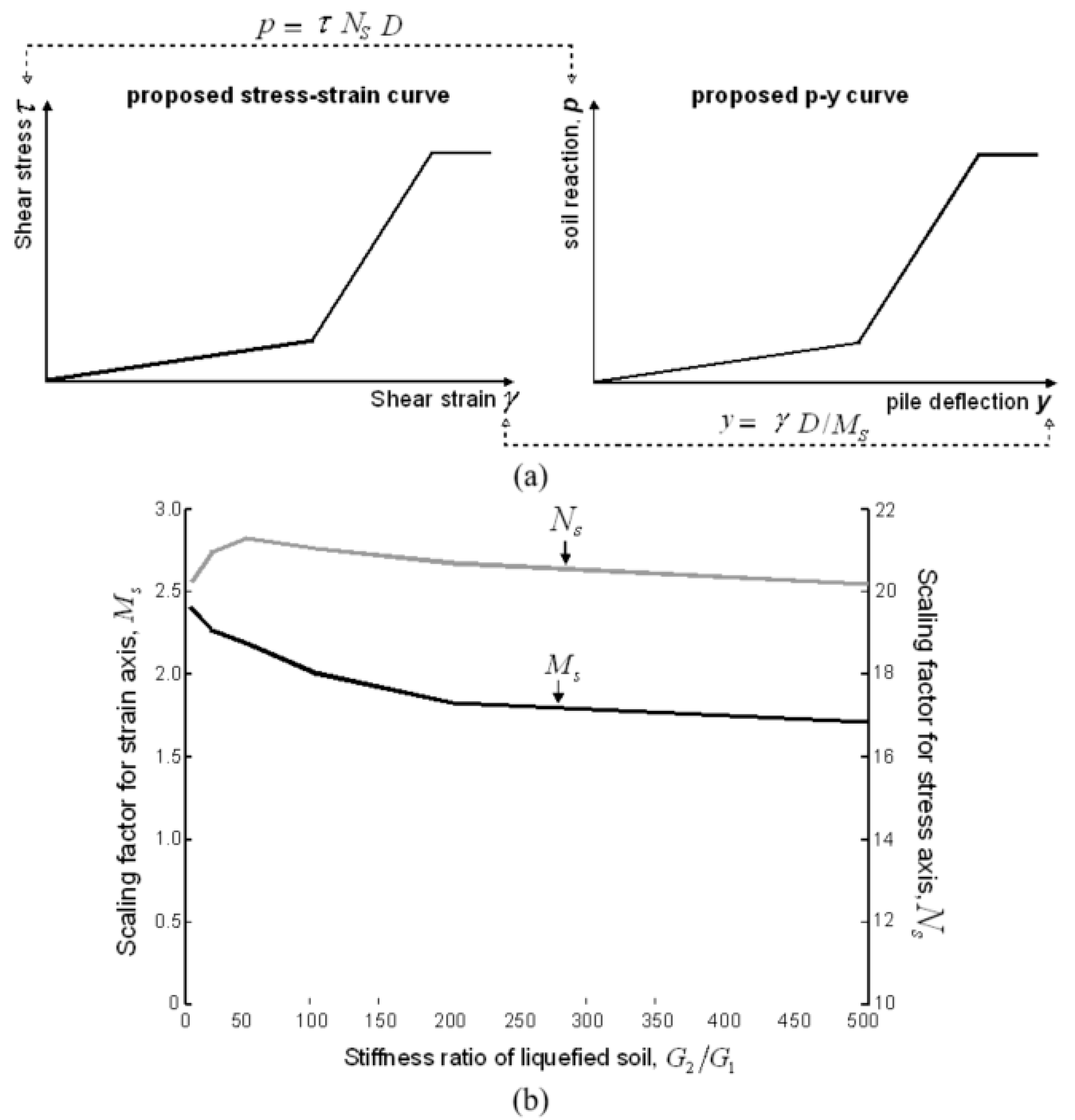
- Once a certain response is observed, the question is how the understanding and findings from the scaled model tests can inform the design method? A possible answer is to use a numerical model that captures the main mechanisms (e.g., reduction of soil strength and stiffness of the liquefied soil) whose input parameters are calibrated based on the experimental results. Different numerical models can be used; however, for the analysis of laterally loaded piles, it may be convenient to use the “beam on nonlinear Winkler foundation” approach in which the soil–structure interaction is modelled by means of springs, which are defined in terms of p–y relationships (see Figure 36). This approach is discussed in more detail below. For the case of liquefied soil, experiments at both normal gravity and multiples of gravity (centrifuge) suggest that the p–y curve has an upward concave shape with an initial flat part (see Figure 37). It is important that the numerical model adopted in the analysis is consistent with the behaviour observed in the experimental studies.
- (c)
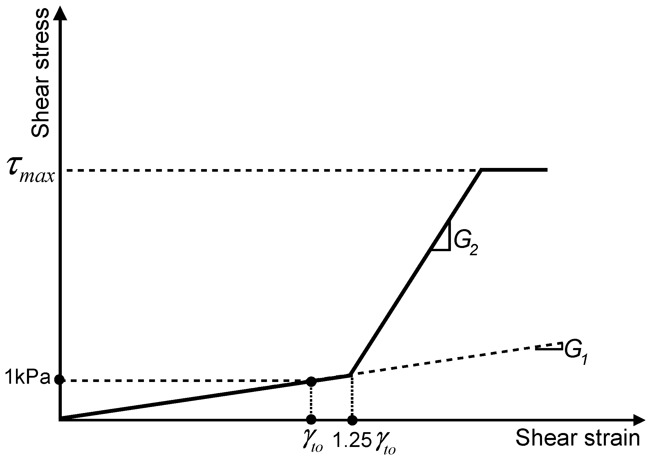
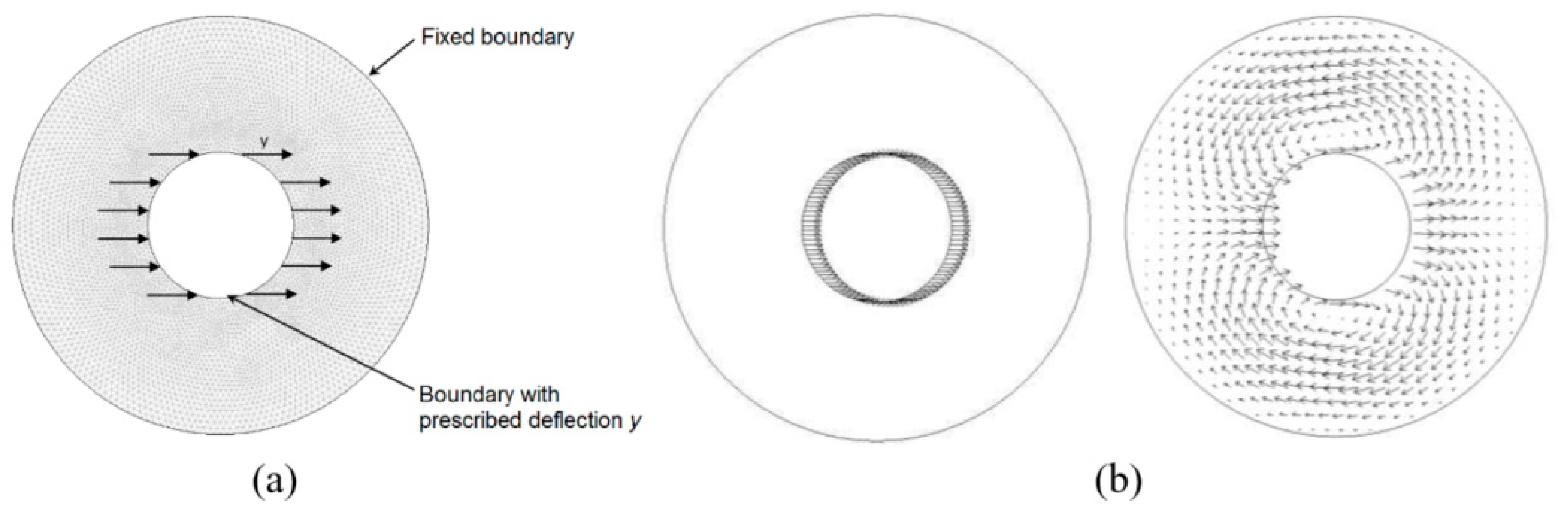
- How can the modeler develop p–y curves that are consistent with the experimental results? This can be carried out by linking results from element tests (triaxial, simple shear) to results from small-scale model tests carried out either at 1× g or in the centrifuge. The readers are referred to [59] for more details on the derivation of the p–y curves for liquefiable soils shown in Figure 36 and Figure 37.
- (d)
- Load-deformation response of the pile, which takes into account the overall macro behavior of the soil–pile system.
- (e)
- Stress–strain response of the adjacent soil being sheared as the pile moves laterally. In theory, the transformation from micro to macro can be made by applying appropriate scaling factors that convert stress into equivalent soil reaction, p, and strain in equivalent relative pile–soil displacement. The scaling factors can be derived from the so-called “Mobilizable Strength Design” (MSD) method [62,63,64]. In routine practice, however, p–y curves are constructed by means of empirical relationships, which were developed during the 1970s and 1980s based on a relatively limited number of full-scale tests carried out on small-diameter steel piles [65,66,67,68,69].
Derivation of Scaling Parameters
- (a)
- Double integration of soil acceleration to compute soil displacement ys. The acceleration can be measured by accelerometers.
- (b)
- Double integration of bending moment along the pile to obtain pile deflection yp. The bending moment can be obtained from strain-gauge pairs installed at different elevations along the foundation.
- (c)
- The relative pile–soil displacement y can be computed as the difference yp-ys;
- (d)
- Double differentiation of bending moment along the pile to obtain soil reaction p.
- (e)
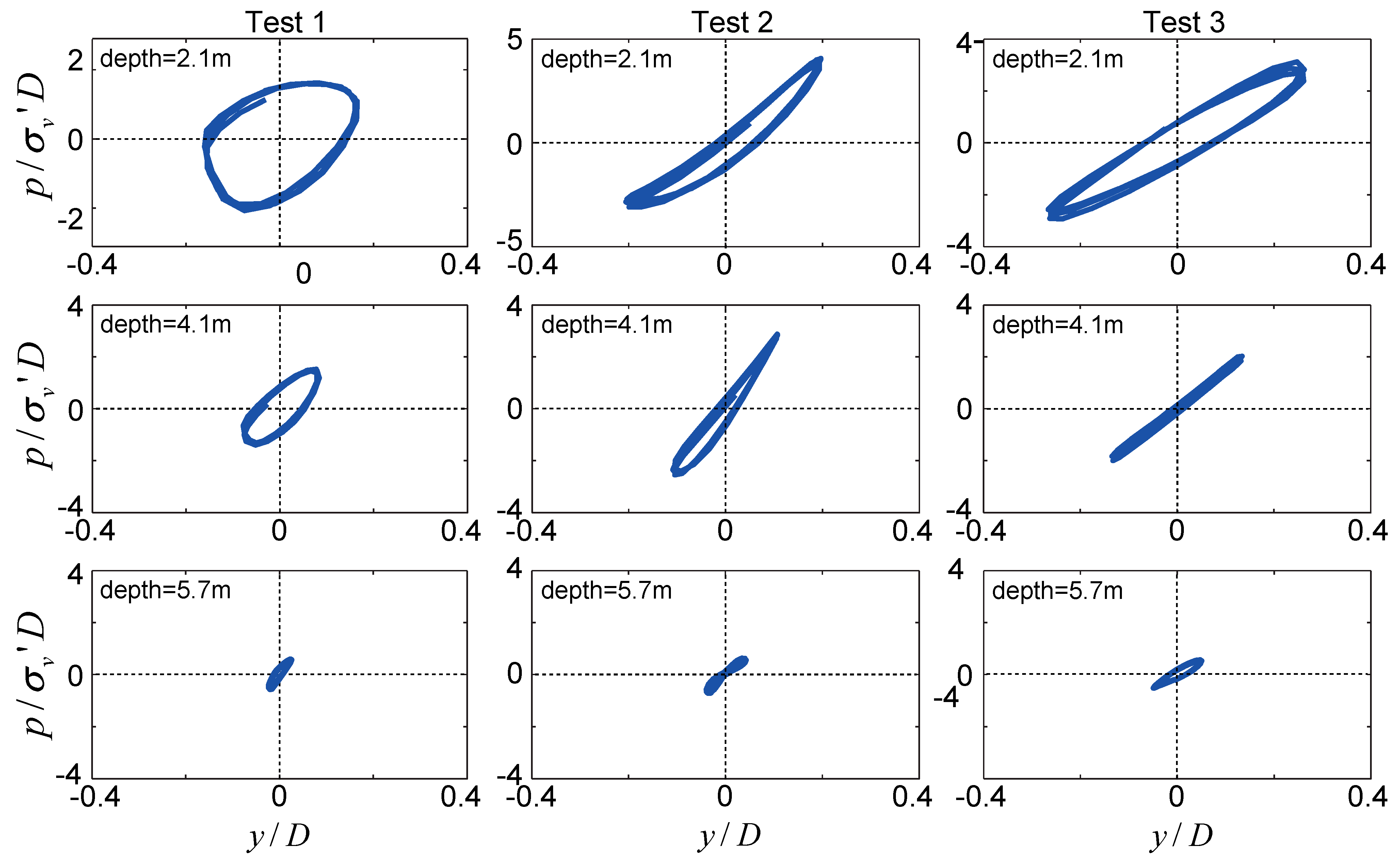
- Figure 43 displays p–y curves relative to three depths within the liquefiable layer (i.e., soil layer 2 in Figure 43). It can be seen that the back-calculated p–y curves exhibited practically zero stiffness at small deflection. The implication of using p–y curves having different shapes was previously discussed through the schematic representation in Figure 37.
- (f)
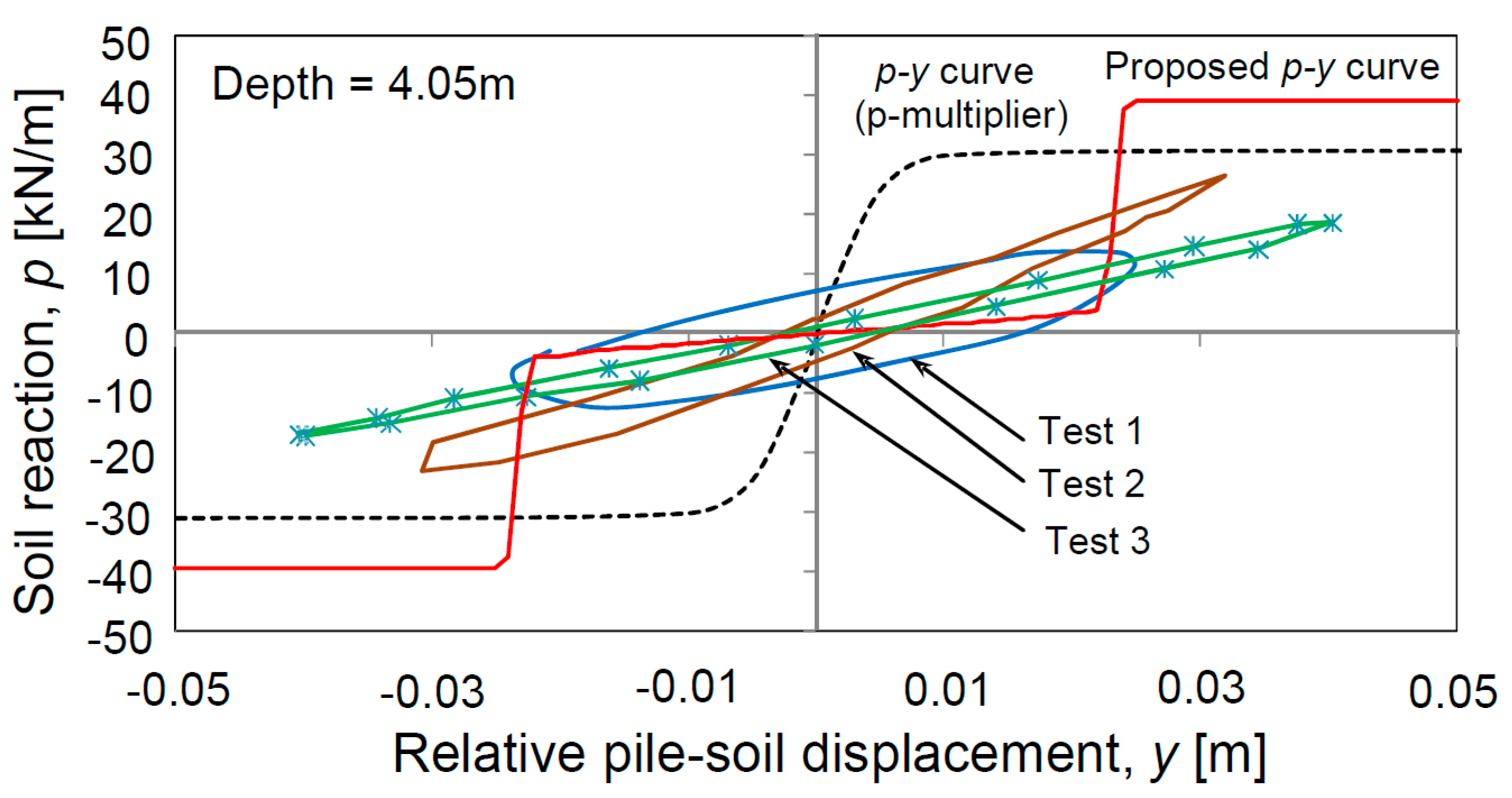
- Figure 44 compares the back-calculated p–y curves with those computed from the proposed and p-multiplier methods. It can be observed that the back-calculated p–y curves exhibit low stiffness at small lateral displacement, and increasing stiffness and lateral resistance with increasing y. This strain-hardening behaviour is better captured by the proposed p–y curves than the routine method, which clearly overestimates the initial foundation stiffness.
8. Discussion and Conclusions
Author Contributions
Funding
Institutional Review Board Statement
Informed Consent Statement
Data Availability Statement
Acknowledgments
Conflicts of Interest
References
- Pagani, M.; Garcia-Pelaez, J.; Gee, R.; Johnson, K.; Poggi, V.; Styron, R.; Weatherill, G.; Simionato, M.; Viganò, D.; Danciu, L.; et al. Global Earthquake Model (GEM): Seismic Hazard Map. Version 2018.1—December 2018. Available online: https://www.preventionweb.net/files/65696_hazardmapcompressed.pdf (accessed on 25 January 2021).
- Bhattacharya, S. Design of Foundations for Offshore Wind Turbines; Wiley: Hoboken, NJ, USA, 2019. [Google Scholar]
- Bhattacharya, S.; Wang, L.; Liu, J.; Hong, Y. Civil engineering challenges associated with design of offshore wind turbines with special reference to China. In Wind Energy Engineering; Academic Press: Cambridge, MA, USA, 2017; pp. 243–273. [Google Scholar]
- Arany, L.; Bhattacharya, S.; Macdonald, J.; Hogan, S.J. Design of monopiles for offshore wind turbines in 10 steps. Soil Dyn. Earthq. Eng. 2017, 92, 126–152. [Google Scholar] [CrossRef]
- Arany, L.; Bhattacharya, S.; Adhikari, S.; Hogan, S.; Macdonald, J.H.G. An analytical model to predict the natural frequency of offshore wind turbines on three-spring flexible foundations using two different beam models. Soil Dyn. Earthq. Eng. 2015, 74, 40–45. [Google Scholar] [CrossRef]
- Bhattacharya, S.; Demirci, H.E.; Nikitas, G.; Prakhya, G.K.V.; Lombardi, D.; Alexander, N.A.; Aleem, M.; Amani, S.; Mylonakis, G. Physical modeling of interaction problems in geotechnical engineering. In Modeling in Geotechnical Engineering; Academic Press: Cambridge, MA, USA, 2021; pp. 205–256. [Google Scholar]
- O’Leary, K.; Pakrashi, V.; Kelliher, D. Optimisation of composite material tower for offshore wind turbine structures. Renew. Energy 2019, 140, 928–942. [Google Scholar] [CrossRef]
- O’Kelly-Lynch, P.; Long, C.; McAuliffe, F.D.; Murphy, J.; Pakrashi, V. Structural design implications of combining a point absorber with a wind turbine monopile for the east and west coast of Ireland. Renew. Sustain. Energy Rev. 2020, 119, 109583. [Google Scholar] [CrossRef]
- O’Donnell, D.; Srbinovsky, B.; Murphy, J.; Popovici, E.; Pakrashi, V. Sensor Measurement Strategies for Monitoring Offshore Wind and Wave Energy Devices. J. Phys. Conf. Ser. 2015, 628, 012117. [Google Scholar] [CrossRef]
- O’Donnell, D.; Murphy, J.; Pakrashi, V. Damage Monitoring of a Catenary Moored Spar Platform for Renewable Energy Devices. Energies 2020, 13, 3631. [Google Scholar] [CrossRef]
- Leimeister, M.; Collu, M.; Kolios, A. A fully integrated optimization framework for designing a complex geometry offshore wind turbine spar-type floating support structure. Wind Energy Sci. Discuss. 2020, 5, 1–35. [Google Scholar] [CrossRef]
- Davidson, C.; Brown, M.J.; Cerfontaine, B.; Al-Baghdadi, T.; Knappett, J.; Brennan, A.; Augarde, C.; Coombs, W.; Wang, L.; Blake, A.; et al. Physical modelling to demonstrate the feasibility of screw piles for offshore jacket-supported wind energy structures. Géotechnique 2020, 1–19. [Google Scholar] [CrossRef]
- Karimi, H.R.; Zapateiro, M.; Luo, N. Semiactive vibration control of offshore wind turbine towers with tuned liquid column dampers using H∞ output feedback control. In Proceedings of the 2010 IEEE International Conference on Control Applications, Yokohama, Japan, 8–10 September 2010; pp. 2245–2249. [Google Scholar]
- Buckley, T.; Watson, P.; Cahill, P.; Jaksic, V.; Pakrashi, V. Mitigating the structural vibrations of wind turbines using tuned liquid column damper considering soil-structure interaction. Renew. Energy 2018, 120, 322–341. [Google Scholar] [CrossRef]
- Jaksic, V.; Wright, C.S.; Murphy, J.; Afeef, C.; Ali, S.F.; Mandic, D.P.; Pakrashi, V. Dynamic response mitigation of floating wind turbine platforms using tuned liquid column dampers. Philos. Trans. R. Soc. A Math. Phys. Eng. Sci. 2015, 373, 20140079. [Google Scholar] [CrossRef]
- Jaksic, V.; O’Shea, R.; Cahill, P.; Murphy, J.; Mandic, D.P.; Pakrashi, V. Dynamic response signatures of a scaled model platform for floating wind turbines in an ocean wave basin. Philos. Trans. R. Soc. A Math. Phys. Eng. Sci. 2015, 373, 20140078. [Google Scholar] [CrossRef] [PubMed]
- Byrne, B.; McAdam, R.; Burd, H.; Houlsby, G.; Martin, C.; Beuckelaers, W.; Zdravkovic, L.; Taborda, D.; Potts, D.; Jardine, R.; et al. PISA: New Design Methods for Offshore Wind Turbine Monopiles. In Proceedings of the Offshore Site Investigation Geotechnics 8th International Conference Proceedings, London, UK, 12–14 September 2017; Society for Underwater Technology: London, UK, 2017; Volume 142, pp. 142–161. [Google Scholar] [CrossRef]
- O’Donnell, D.; Murphy, J.; Pakrashi, V. Comparison of Response Amplitude Operator Curve Generation Methods for Scaled Floating Renewable Energy Platforms in Ocean Wave Basin. ASME Lett. Dyn. Syst. Control 2021, 1, 021012. [Google Scholar] [CrossRef]
- O’Byrne, M.; Schoefs, F.; Pakrashi, V.; Ghosh, B. An underwater lighting and turbidity image repository for analysing the performance of image-based non-destructive techniques. J. Struct. Infrastruct. Eng. 2018, 14, 104–123. [Google Scholar] [CrossRef]
- Benreguig, P.; Kelly, J.; Pakrashi, V.; Murphy, J. Wave-to-Wire model development and validation for Two OWC type wave energy converters. Energies 2019, 12, 3977. [Google Scholar] [CrossRef]
- Benreguig, P.; Pakrashi, V.; Murphy, J. Assessment of Primary Energy Conversion of a Closed-Circuit OWC Wave Energy Converter. Energies 2019, 12, 1962. [Google Scholar] [CrossRef]
- Malekjafarian, A.; Jalilvand, S.; Doherty, P.; Igoe, D. Foundation damping for monopile supported offshore wind turbines: A review. Mar. Struct. 2021, 77, 102937. [Google Scholar] [CrossRef]
- Adhikari, S.; Bhattacharya, S. A general frequency adaptive framework for damped response analysis of wind turbines. Soil Dyn. Earthq. Eng. 2021, 143, 106605. [Google Scholar] [CrossRef]
- Bhattacharya, S.; Lombardi, D.; Wood, D.M. Similitude relationships for physical modelling of mono-pile-supported offshore wind turbines. Int. J. Phys. Model. Geotech. 2011, 11, 58–68. [Google Scholar]
- Bhattacharya, S.; Nikitas, N.; Garnsey, J.; Alexander, N.; Cox, J.; Lombardi, D.; Wood, D.M.; Nash, D. Observed dynamic soil–structure interaction in scale testing of offshore wind turbine foundations. Soil Dyn. Earthq. Eng. 2013, 54, 47–60. [Google Scholar] [CrossRef]
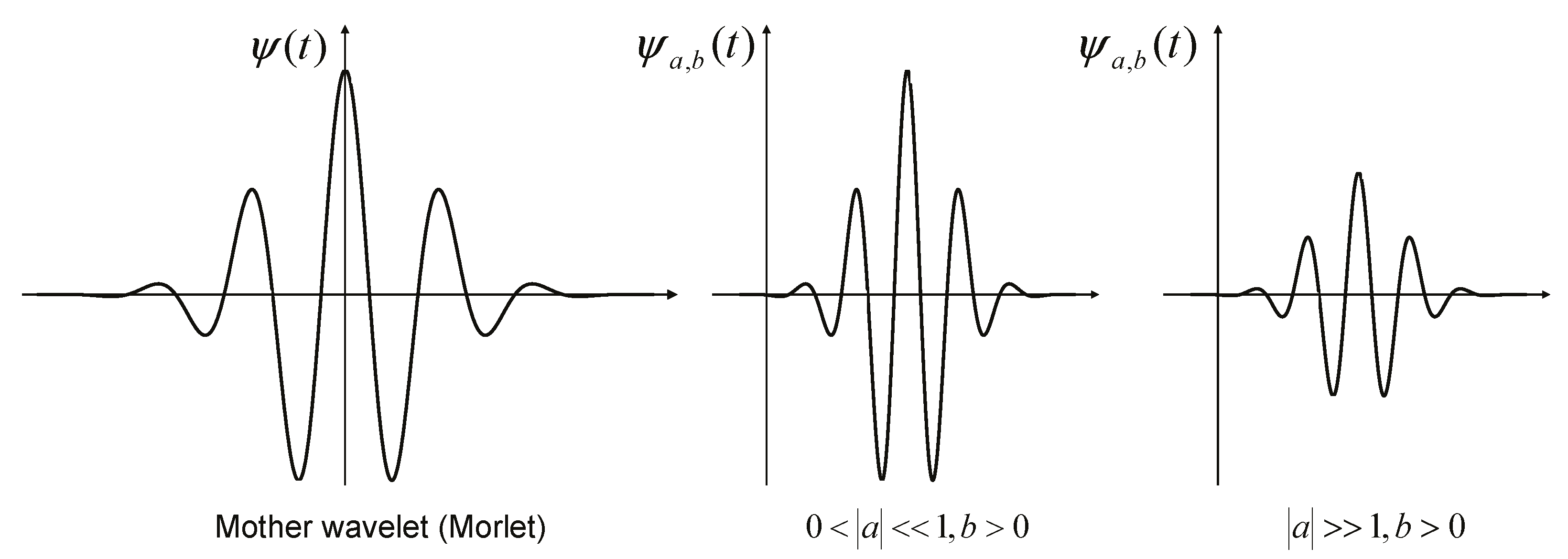
- Hall, F.; Lombardi, D.; Bhattacharya, S. Identification of transient vibration characteristics of pile-group models during liquefaction using wavelet transform. Eng. Struct. 2018, 171, 712–729. [Google Scholar] [CrossRef]
- Adhikari, S.; Bhattacharya, S. Vibrations of wind-turbines considering soil-structure interaction. Wind. Struct. 2011, 14, 85–112. [Google Scholar] [CrossRef]
- Jalbi, S.; Arany, L.; Salem, A.; Cui, L.; Bhattacharya, S. A method to predict the cyclic loading profiles (one-way or two-way) for monopile supported offshore wind turbines. Mar. Struct. 2019, 63, 65–83. [Google Scholar] [CrossRef]
- Jalbi, S.; Bhattacharya, S. A comparison between advanced and simplified methods to predict the natural frequency of offshore wind turbines incorporating soil-structure interaction. Coast. Struct. 2019, 2019, 904–912. [Google Scholar]
- Lombardi, D.; Bhattacharya, S.; Wood, D.M. Dynamic soil–structure interaction of monopile supported wind tur-bines in cohesive soil. Soil Dyn. Earthq. Eng. 2013, 49, 165–180. [Google Scholar] [CrossRef]
- Nikitas, G.; Vimalan, N.J.; Bhattacharya, S. An innovative cyclic loading device to study long term performance of offshore wind turbines. Soil Dyn. Earthq. Eng. 2016, 82, 154–160. [Google Scholar] [CrossRef]
- Yu, L.-Q.; Wang, L.-Z.; Guo, Z.; Bhattacharya, S.; Nikitas, G.; Li, L.-L.; Xing, Y.-L. Long-term dynamic behavior of monopile supported offshore wind turbines in sand. Theor. Appl. Mech. Lett. 2015, 5, 80–84. [Google Scholar] [CrossRef]
- Guo, Z.; Yu, L.; Wang, L.; Bhattacharya, S.; Nikitas, G.; Xing, Y. Model Tests on the Long-Term Dynamic Performance of Offshore Wind Turbines Founded on Monopiles in Sand. J. Offshore Mech. Arct. Eng. 2015, 137, 041902. [Google Scholar] [CrossRef]
- Xu, Y.; Nikitas, G.; Zhang, T.; Han, Q.; Chryssanthopoulos, M.; Bhattacharya, S.; Wang, Y. Support condition monitoring of offshore wind turbines using model updating techniques. Struct. Health Monit. 2020, 19, 1017–1031. [Google Scholar] [CrossRef]
- Lombardi, D.; Bhattacharya, S. Evaluation of seismic performance of pile-supported models in liquefiable soils. Earthq. Eng. Struct. Dyn. 2016, 45, 1019–1038. [Google Scholar] [CrossRef]
- Lombardi, D. Dynamics of Pile-Supported Structures in Seismically Liquefiable Soils. Ph.D. Thesis, University of Bristol, Bristol, UK, 2014. [Google Scholar]
- Lombardi, D.; Bhattacharya, S.; Hyodo, M.; Kaneko, T. Undrained behaviour of two silica sands and practical implications for modelling SSI in liquefiable soils. Soil Dyn. Earthq. Eng. 2014, 66, 293–304. [Google Scholar] [CrossRef]
- Jaksic, V.; Wright, C.; Mandic, D.P.; Murphy, J.; Pakrashi, V. A delay vector variance based marker for an output-only assessment of structural changes in tension leg platforms. J. Phys. Conf. Ser. 2015, 628, 012059. [Google Scholar] [CrossRef]
- Arany, L.; Bhattacharya, S. Simplified load estimation and sizing of suction anchors for spar buoy type floating offshore wind turbines. Ocean Eng. 2018, 159, 348–357. [Google Scholar] [CrossRef]
- Welch, P. The use of fast Fourier transform for the estimation of power spectra: A method based on time averaging over short, modified periodograms. IEEE Trans. Audio Electroacoust. 1967, 15, 70–73. [Google Scholar] [CrossRef]
- Bhattacharya, S.; Cox, J.A.; Lombardi, D.; Wood, D.M. Dynamics of offshore wind turbines supported on two foundations. Proc. Inst. Civ. Eng. Geotech. Eng. 2013, 166, 159–169. [Google Scholar] [CrossRef]
- Cox, J.A.; O’Loughlin, C.; Cassidy, M.; Bhattacharya, S.; Gaudin, C.; Bienen, B. Centrifuge study on the cyclic performance of caissons in sand. Int. J. Phys. Model. Geotech. 2014, 14, 99–115. [Google Scholar] [CrossRef]
- Bhattacharya, S.; Lombardi, D.; Dihoru, L.; Dietz, M.S.; Crewe, A.J.; Taylor, C.A. Model container design for soil-structure interaction studies. In Role of Seismic Testing Facilities in Performance-Based Earthquake Engineering; Springer: Dordrecht, The Netherlands, 2012; pp. 135–158. [Google Scholar]
- Lombardi, D.; Bhattacharya, S.; Scarpa, F.; Bianchi, M. Dynamic response of a geotechnical rigid model container with absorbing boundaries. Soil Dyn. Earthq. Eng. 2015, 69, 46–56. [Google Scholar] [CrossRef]
- Kolsky, H. Stress Waves in Solids; Clarendon Press: Oxford, UK, 1953. [Google Scholar]
- Cohen, L. Time-Frequency Analysis; Prentice-Hall: Englewood Cliffs, NJ, USA, 1995. [Google Scholar]
- Simpson, J.J. Oceanographic and atmospheric applications of spatial statistics and digital image analysis. In Spatial Statistics and Digital Image Analysis; National Academy Press: Washington, DC, USA, 1991. [Google Scholar]
- Huang, N.E.; Shen, Z.; Long, S.R.; Wu, M.C.; Shih, H.H.; Zheng, Q.; Yen, N.C.; Tung, C.C.; Liu, H.H. The empirical mode decomposition and the Hilbert spectrum for non-linear and non-stationary time series analysis. Philos. Trans. R. Soc. A Math. Phys. Eng. Sci. 1991, 454, 903–995. [Google Scholar] [CrossRef]
- Huang, N.E.; Wu, Z. A review on Hilbert-Huang transform: Method and its applications to geophysical studies. Rev. Geophys. 2008, 46, 1–23. [Google Scholar] [CrossRef]
- Morlet, J.; Arens, G.; Fourgeau, E.; Glard, D. Wave propagation and sampling theory—Part I: Complex signal and scattering in multilayered media. Geophysics 1982, 47, 203–221. [Google Scholar] [CrossRef]
- Gurley, K.; Kareem, A. Applications of wavelet transforms in earthquake, wind and ocean engineering. Eng. Struct. 1999, 21, 149–167. [Google Scholar]
- Chakraborty, A.; Okaya, D. Frequency-time decomposition of seismic data using wavelet-based methods. Geophysics 1995, 60, 1906–1916. [Google Scholar] [CrossRef]
- Basu, B.; Gupta, V.K. Stochastic seismic response of single-degree-of-freedom systems through wavelets. Eng. Struct. 2000, 22, 1714–1722. [Google Scholar] [CrossRef]
- Lombardi, D.; Bhattacharya, S. Modal analysis of pile-supported structures during seismic liquefaction. Earthq. Eng. Struct. Dyn. 2014, 43, 119–138. [Google Scholar] [CrossRef]
- Lombardi, D. Dynamics of Offshore Wind Turbines; University of Bristol: Bristol, UK, 2010. [Google Scholar]
- Iyama, J.; Kuwamura, H. Application of wavelets to analysis and simulation of earthquake motions. Earthq. Eng. Struct. Dyn. 1999, 28, 255–272. [Google Scholar] [CrossRef]
- Jalbi, S.; Nikitas, G.; Bhattacharya, S.; Alexander, N. Dynamic design considerations for offshore wind turbine jackets supported on multiple foundations. Mar. Struct. 2019, 67, 102631. [Google Scholar] [CrossRef]
- Jalbi, S.; Bhattacharya, S. Minimum foundation size and spacing for jacket supported offshore wind turbines considering dynamic design criteria. Soil Dyn. Earthq. Eng. 2019, 123, 193–204. [Google Scholar] [CrossRef]
- Dash, S.; Rouholamin, M.; Lombardi, D.; Bhattacharya, S. A practical method for construction of p-y curves for liquefiable soils. Soil Dyn. Earthq. Eng. 2017, 97, 478–481. [Google Scholar] [CrossRef]
- Winkler, E. Die Lehre von der Elasticitaet und Festigkeit Besonderer Rucksicht auf ihre Anwendung in der Technik fur Politechniche Schulen, Bauakademien, Ingenieure, Maschinenbauer, Architecten, etc. 1867. Available online: https://archive.org/details/bub_gb_25E5AAAAcAAJ (accessed on 26 May 2021).
- Hetényi, M. Beams on Elastic Foundation: Theory with Applications in the Fields of Civil and Mechanical Engineering; The University of Michigan Press: Ann Arbor, MI, USA, 1946. [Google Scholar]
- Bouzid, D.J.; Bhattacharya, S.; Dash, S.R. Winkler Springs (p-y curves) for pile design from stress-strain of soils: FE assessment of scaling coefficients using the Mobilised Strength Design concept. Geomech. Eng. 2013, 5, 379–399. [Google Scholar] [CrossRef]
- Bolton, M.D.; Powrie, W. Behavior of diaphragm walls in clay prior to collapse. Géotechnique 1988, 38, 167–189. [Google Scholar] [CrossRef]
- Osman, A.S.; Bolton, M.D. A new design method for retaining walls in clay. Can. Geotech. J. 2004, 41, 451–466. [Google Scholar] [CrossRef]
- Matlock, H. Correlation for design of laterally loaded piles in soft clay. In Proceedings of the Offshore Technology Conference, Houston, TX, USA, 21–23 April 1970; pp. 77–94. [Google Scholar]
- Reese, L.C.; Cox, W.R.; Koop, F.D. Analysis of Laterally Loaded Piles in Sand. In Proceedings of the Offshore Technology Conference, Houston, TX, USA, 5–7 May 1974; Volume 2. [Google Scholar]
- Reese, L.C.; Cox, W.R.; Koop, F.D. Field Testing and Analysis of Laterally Loaded Piles in Stiff Clay. In Proceedings of the Offshore Technology Conference, Houston, TX, USA, 5–7 May 1975. [Google Scholar]
- O’Neill, M.W.; Murchison, J.M. An Evaluation of p-y Relationships in Sands; Report to American Petroleum Institute; University of Texas at Austin: Austin, TX, USA, 1983. [Google Scholar]
- Aleem, M.; Demirci, H.E.; Bhattacharya, S. Lateral and Moment Resisting Capacity of Monopiles In Layered Soils. In Proceedings of the ICEESEN, Kayseri, Turkey, 19 November 2020; pp. 19–21. [Google Scholar]
- Dash, S. Lateral Pile-Soil Interaction in Liquefiable Soils. Ph.D. Thesis, University of Oxford, Oxford, UK, 2010. [Google Scholar]
- Randolph, M.F.; Houlsby, G.T. The limiting pressure on a circular pile loaded laterally in cohesive soil. Géotechnique 1984, 34, 613–623. [Google Scholar] [CrossRef]
- Sato, M. A new dynamic geotechnical centrifuge and performance of shaking table tests. Int. Conf. Cent. 1994, 94, 157–162. [Google Scholar]


| TRL Level as European Commission | Interpretation of the Terminology and Remarks |
|---|---|
| TRL-1: Basic principles verified | It necessary to verify that the governing mechanics principles are obeyed. For example, in the case of foundations, it must be checked whether the whole system is in equilibrium under the action of environmental loads. |
| TRL-2: Technology concept formulated | It is necessary to assess the whole technology starting from fabrication to methods of installation, and operation and maintenance (O&M), and decommissioning. In this step, it is expected that method statements will be developed. |
| TRL-3: Experimental proof of concept | Small-scale models need to tested to verify steps in TRL-1 and TRL-2. In terms of foundation, this would correspond to checking the modes of failure in Ultimate Limit State (ULS) and identifying the modes of vibration. |
| TRL-4: Technology validated in lab | Once TRL-3 is satisfied and the business decision is taken to go ahead with the development/design, it is necessary to determine that the proposed technology is sound under the most likely scenarios encountered during the operation of the wind turbine. This may include long-term performance under millions of cycles of loading and evaluate the dynamic performance over the lifetime in relation to Serviceability Limit State (SLS) Fatigue Limit State (FLS). |
| TRL-5 Technology validated in relevant environment | Validation in a relevant environment may require further numerical simulation in which models are calibrated based on the results from the small-scale model tests and element tests. In the context of foundation, this step may use advanced soil constitutive models to verify the performance under extreme loading. |
| TRL-6: Technology demonstrated in relevant environment | To demonstrate the technology in the relevant environment, a prototype foundation may need to be constructed and tested in the offshore environment representative of the real site conditions. |
| TRL-7: System prototype demonstration in operational environment | The foundation is subjected to operational loads, and the performance is monitored. |
| TRL-8: System complete and qualified | Based on the results in TRL-7, the system can be classified as qualified or not qualified, or changes are required. |
| TRL-9: Actual system proven in operational environment | Technology may be used in energy generation with contingency plans. |
| Types of Testing | Remarks on the Understanding |
|---|---|
| Wind Tunnel testing | Blades can be tested to show the importance of profile. |
| Wave Tank Testing | Wave tank of different forms can be used to study scour, hydrodynamic loading, tsunami. |
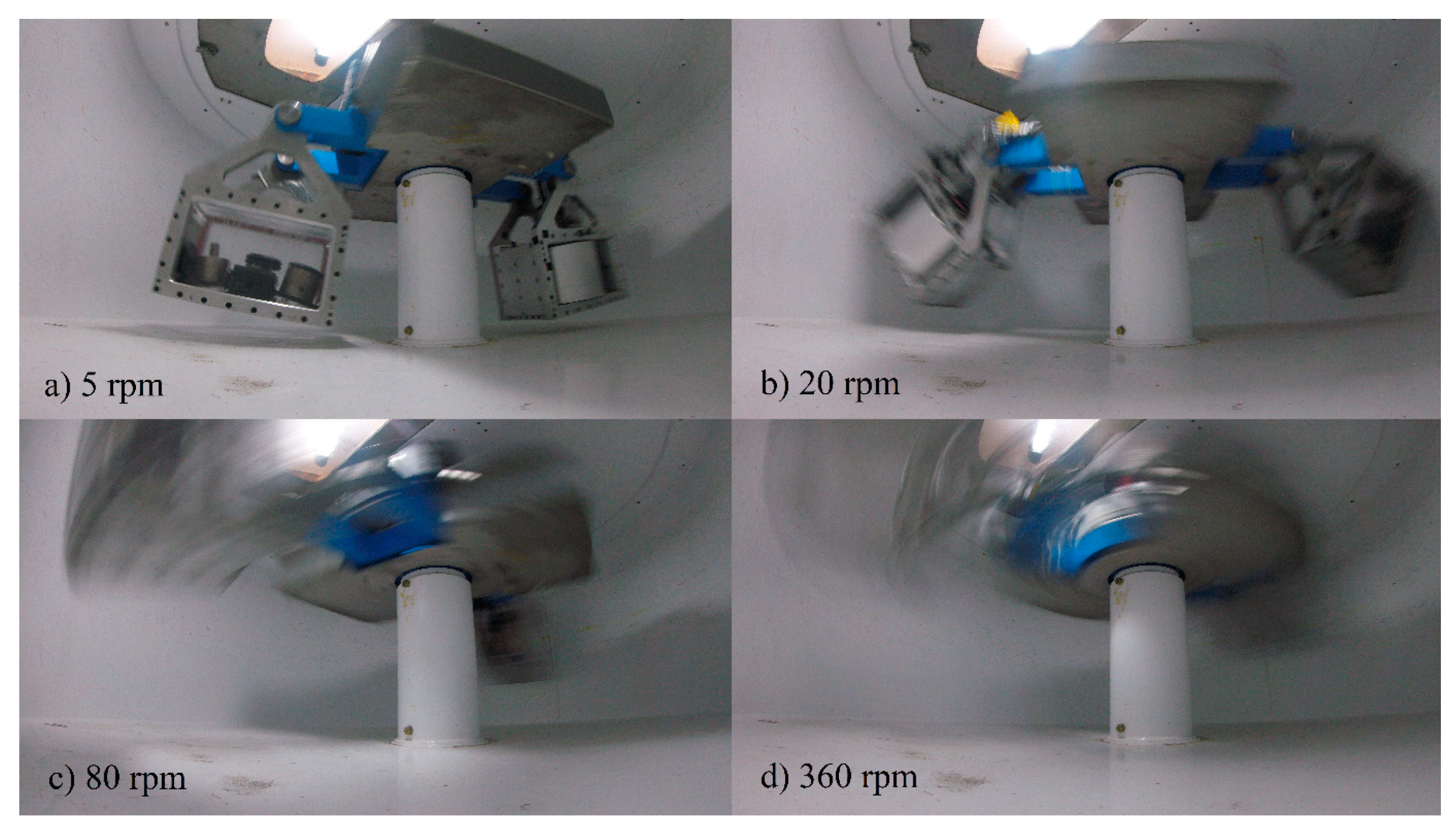
| Geotechnical Centrifuge | Geotechnical centrifuge enables replication of the stress levels that the soil experiences in the field. However, the whole model is spun at a high rate which creates unwanted small vibrations. Therefore, the subtle dynamics of the problem is difficult to study as filtering of signals are inevitable during the processing of data. |
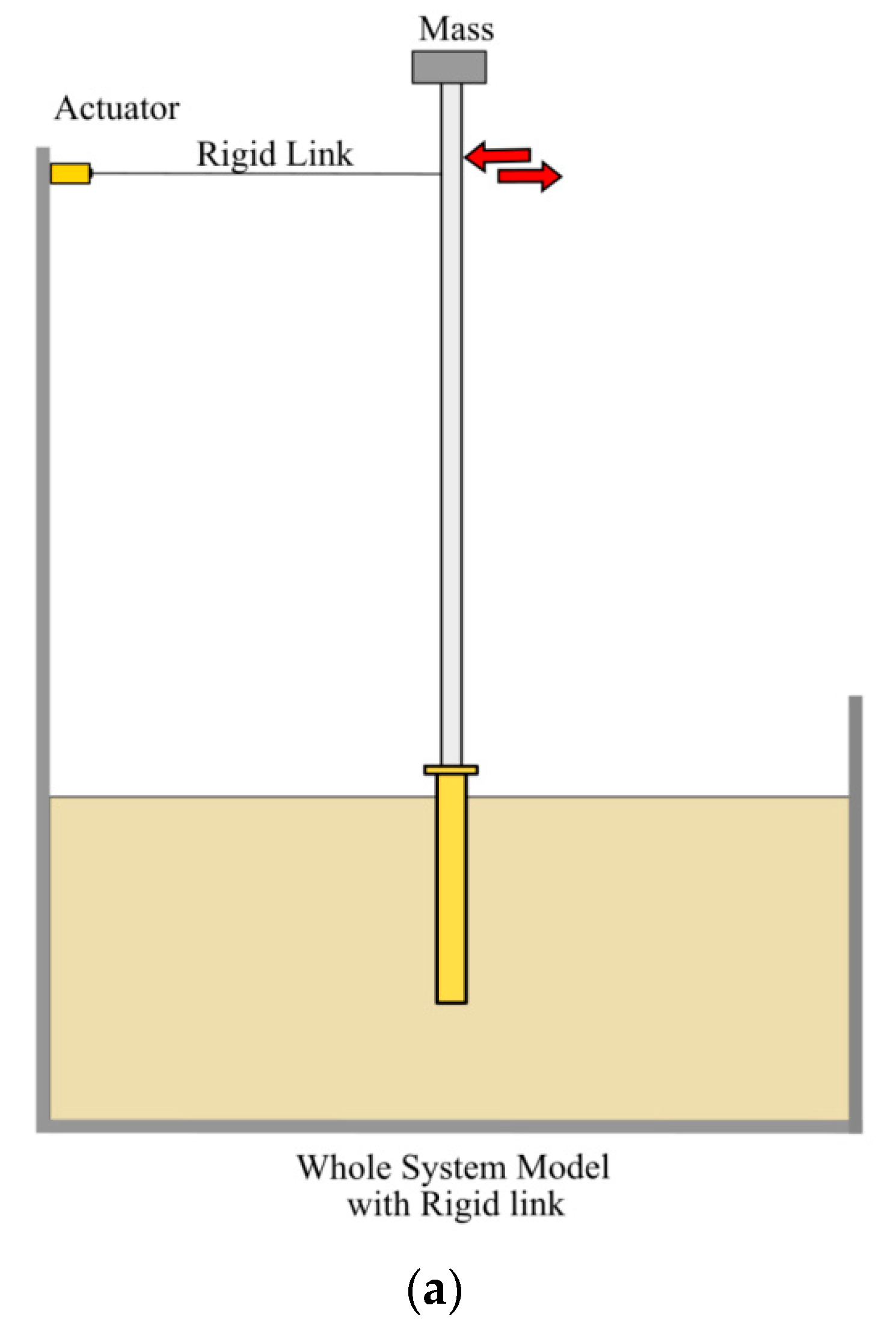
| Whole System modelling | Small-scale whole system modelling, which can be considered as a full-scale prototype pioneered by [24], is one approach to studying the overall system. This type of modelling was used to carry out TRL of a Self-Installing Wind Turbine (SIWT) asymmetric tripod; details are provided in [25]. Because the system is tested on a stable floor, dynamics of the problem can be readily studied. Further details can be found in [6]. |
Publisher’s Note: MDPI stays neutral with regard to jurisdictional claims in published maps and institutional affiliations. |
© 2021 by the authors. Licensee MDPI, Basel, Switzerland. This article is an open access article distributed under the terms and conditions of the Creative Commons Attribution (CC BY) license (https://creativecommons.org/licenses/by/4.0/).
Share and Cite
Bhattacharya, S.; Lombardi, D.; Amani, S.; Aleem, M.; Prakhya, G.; Adhikari, S.; Aliyu, A.; Alexander, N.; Wang, Y.; Cui, L.; et al. Physical Modelling of Offshore Wind Turbine Foundations for TRL (Technology Readiness Level) Studies. J. Mar. Sci. Eng. 2021, 9, 589. https://doi.org/10.3390/jmse9060589
Bhattacharya S, Lombardi D, Amani S, Aleem M, Prakhya G, Adhikari S, Aliyu A, Alexander N, Wang Y, Cui L, et al. Physical Modelling of Offshore Wind Turbine Foundations for TRL (Technology Readiness Level) Studies. Journal of Marine Science and Engineering. 2021; 9(6):589. https://doi.org/10.3390/jmse9060589
Chicago/Turabian StyleBhattacharya, Subhamoy, Domenico Lombardi, Sadra Amani, Muhammad Aleem, Ganga Prakhya, Sondipon Adhikari, Abdullahi Aliyu, Nicholas Alexander, Ying Wang, Liang Cui, and et al. 2021. "Physical Modelling of Offshore Wind Turbine Foundations for TRL (Technology Readiness Level) Studies" Journal of Marine Science and Engineering 9, no. 6: 589. https://doi.org/10.3390/jmse9060589
APA StyleBhattacharya, S., Lombardi, D., Amani, S., Aleem, M., Prakhya, G., Adhikari, S., Aliyu, A., Alexander, N., Wang, Y., Cui, L., Jalbi, S., Pakrashi, V., Li, W., Mendoza, J., & Vimalan, N. (2021). Physical Modelling of Offshore Wind Turbine Foundations for TRL (Technology Readiness Level) Studies. Journal of Marine Science and Engineering, 9(6), 589. https://doi.org/10.3390/jmse9060589