Installation of Large-Diameter Monopiles: Introducing Wave Dispersion and Non-Local Soil Reaction

Abstract

During the last decade the offshore wind industry grew ceaselessly and engineering challenges continuously arose in that area. Installation of foundation piles, known as monopiles, is one of the most critical phases in the construction of offshore wind farms. Prior to installation a drivability study is performed, by means of pile driving models. Since the latter have been developed for small-diameter piles, their applicability for the analysis of large-diameter monopiles is questionable. In this paper, a three-dimensional axisymmetric pile driving model with non-local soil reaction is presented. This new model aims to capture properly the propagation of elastic waves excited by impact piling and address non-local soil reaction. These effects are not addressed in the available approaches to predict drivability and are deemed critical for large-diameter monopiles. Predictions of the new model are compared to those of a one-dimensional model typically used nowadays. A numerical study is performed to showcase the disparities between the two models, stemming from the effect of wave dispersion and non-local soil reaction. The findings of this numerical study affirmed the significance of both mechanisms and the need for further developments in drivability modeling, notably for large-diameter monopiles.

1. Introduction

In the area of renewable energy, offshore wind occupies an eminent position. Since the onset of offshore wind farm construction, monopiles constitute the dominant foundation concept used in shallow and intermediate water depths [1,2]. Installation of monopile foundations for offshore wind turbines (OWTs) is a considerably challenging operation and the associated cost comprises a significant part of the total budget for an offshore wind farm [3,4]. For that reason, in the design stage, close attention is required to various aspects, one of which is the analysis of pile drivability. Inaccurate pile drivability predictions can cause time delays, excessive financial costs, or even greater project risks, e.g., pile refusal [5]. Thus, it is evident that reliable numerical tools are needed for pile driving analysis, primarily for offshore monopiles due to the aforementioned possible complications. As a consequence of ceaseless advancements in offshore wind in recent years [6], the monopiles used as foundations for OWTs have increased in both length and diameter, and their installation process has raised various challenges.

For the prediction of pile drivability, an analysis is performed that takes into account the pile characteristics, the soil profile at the location of installation and the impact/vibratory hammer to drive the pile to the required depth [7]. The vast majority of pile driving models used in engineering practice are based on the model proposed by Smith [8]; a one-dimensional model that describes the pile by a system of linear springs and masses and the soil reaction by elasto-plastic springs and viscous dashpots. Subsequently, various modifications have been proposed towards rational pile driving models, by improving certain aspects of Smith’s model, such as the empirical character of the soil reaction parameters [9,10]. For that purpose, dynamic models that represent the linear soil reaction, based on analytical formulations [11,12], have been used in conjunction with non-linear relations to account for the pile penetration process (pile slip). However, the linear part of these formulations, expressed in terms of fundamental soil properties, is frequency-dependent. The latter fact is usually overlooked in pile driving analysis and frequency-independent values are assigned to these elements, in order to facilitate the numerical simulations in the time domain. As a result, local and frequency-independent springs and dashpots are arranged together with non-linear elements, e.g., frictional sliders, to represent the soil reaction during installation. Evidently, the above-discussed approaches comprised significant steps towards less empirical, rational pile driving models.

In the advent of large-diameter monopiles, used in offshore wind, the validity of the existing approaches to analyse pile drivability was examined. In [13], the applicability of the available design approaches to compute the static resistance to driving (SRD) was investigated, since these approaches are largely empirical and were developed for piles of relatively small diameter (less than 2 m) [13,14]. Furthermore, Byrne et al. [13] introduced a modification factor in the aforementioned approaches, which resulted in improved and adequate drivability predictions. However, in a subsequent extensive study [15], both the existing and the modified approaches were proved not to provide reliable predictions of the blow counts.

Albeit the above-discussed works focused mainly on determination of the SRD and its influence on drivability predictions, other aspects of available pile driving models have also been examined. Due to the increase of the diameter of monopiles, various works questioned the validity of the classical rod theory, which is exclusively used to describe the pile dynamics during installation [16,17]. Since the spectrum of frequencies excited in the pile during a hammer impact may pertain in the range in which dispersive effects are not negligible, a more accurate description of the pile structure is required. In these structures, frequencies in the vicinity of the ring frequency correspond to predominantly radial motions [18], which cannot be addressed in current models and are related to strong Poisson effects that can significantly affect the soil reaction along the pile shaft [19].

In view of the existing knowledge gaps, a three-dimensional axisymmetric model is developed herein, as a step towards pile driving models suitable for large-diameter monopiles. The phenomenon of wave dispersion is treated directly by modelling the pile as a cylindrical shell according to the Love-Timoshenko thin shell theory. Furthermore the effect of non-local dynamic soil reaction is introduced, by formulating a non-local foundation model based on the stiffness and damping parameters of its local counterpart. To demonstrate the effects of the aforementioned mechanisms, a one-dimensional pile driving model with local soil reaction, as customarily used in engineering practice, is formulated and a numerical study is performed to compare the two approaches. It is observed that pile penetration is significantly affected by wave dispersion, while with ascending diameter the effect becomes more prominent. Non-locality showcases also a stronger deviation from the responses of local reaction models for large diameters. Since for large-diameter cases, both examined mechanisms significantly alter the drivability predictions of standard approaches, their incorporation in pile driving models for large-diameter monopiles is deemed critical.

The paper is structured as follows. In Section 2 the description of the one-dimensional pile driving model and the non-local three-dimensional model are given. The comparison of the results obtained from the two approaches is presented in Section 3, highlighting the effects of wave dispersion and non-local reaction for various cases. Conclusively, in Section 4 the findings are discussed, alongside with the importance of the introduced effects and insights for further development.

2. Modelling of Pile Driving

In Section 2.1 a one-dimensional pile driving model is developed, based on approaches widely used in engineering practice. Wave propagation in thin cylindrical shells is discussed in Section 2.2, accompanied by the development of a three-dimensional axisymmetric model with non-local soil reaction. Details about the numerical solution of the two models are given in Section 2.3.

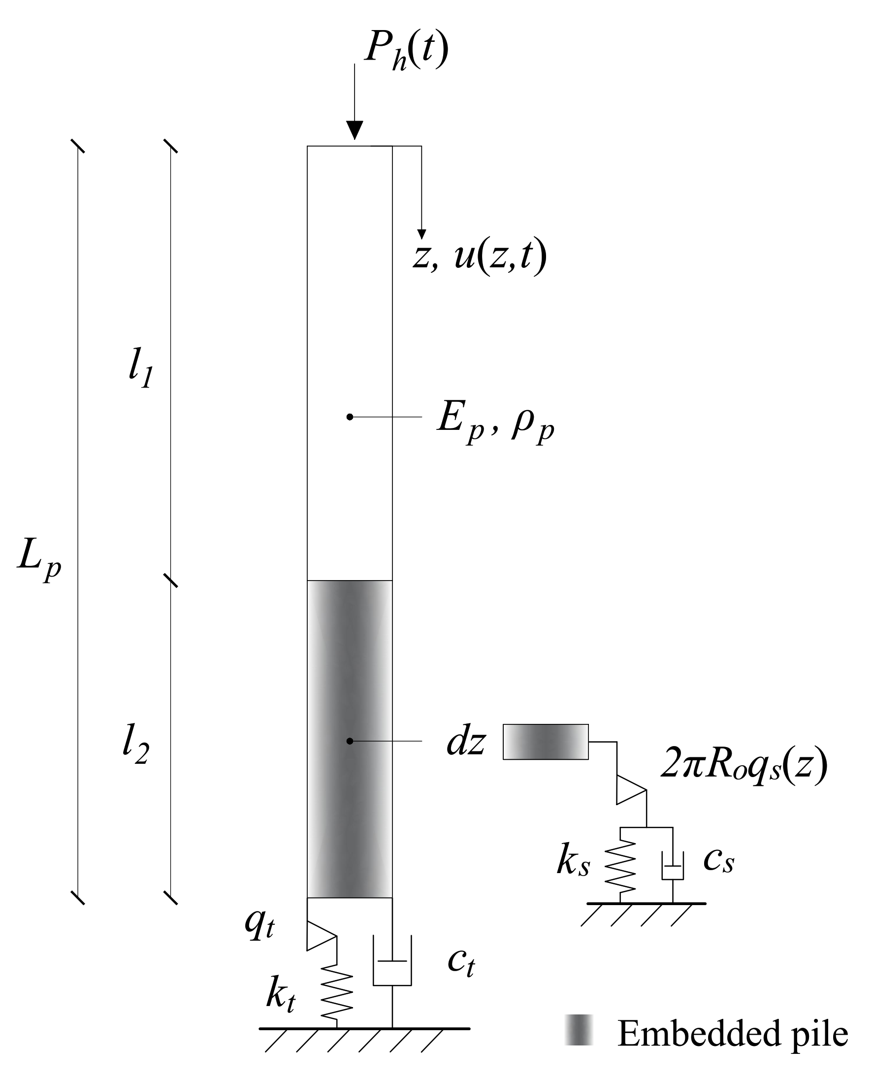
2.1. One-Dimensional Pile Driving Model

The open-ended pile is modelled as a linear homogeneous elastic rod occupying the domain $0\le z\le L_p$, where $L_p$ denotes the length of the pile as displayed in Figure 1. The soil reaction is represented by a combination of elastic springs, viscous dashpots and plastic sliders, as described below in the paper. The equation of motion of the rod reads:

$${\displaystyle {\rho }_p{A}_p\frac{{\partial }^{2}u(z,t)}{\partial t^2}=E_p{A}_p\frac{{\partial }^{2}u(z,t)}{\partial z^2}-H(z-l_1)p_s}$$

(1)

in which ${\rho }_p$ is the mass density of the pile, $A_p$ is the area of the pile cross-section, $u(z,t)$ is the axial displacement of the pile, which is a function of the spatial coordinate z and time t, $E_p$ is the Young’s modulus of the pile, $H(·)$ is the Heaviside function, $l_1$ is the non-embedded pile length and $p_s$ is the soil resistance along the pile shaft. The latter is defined as [9]:

$$p_s=\left\{\begin{array}{cc}{\displaystyle k_s\left(u(z,t)-u_{eq,s}(z,t)\right)+c_s\frac{\partial u(z,t)}{\partial t},}\hfill & {\displaystyle \mathrm{for}\left|k_s\left(u(z,t)-u_{eq,s}(z,t)\right)+c_s\frac{\partial u(z,t)}{\partial t}\right|\le 2\pi R_o{q}_s\left(z\right)}\hfill \\ {\displaystyle 2\pi R_o{q}_s\left(z\right)sgn\left(\frac{\partial u(z,t)}{\partial t}\right),}\hfill & {\displaystyle \mathrm{for}\left|k_s\left(u(z,t)-u_{eq,s}(z,t)\right)+c_s\frac{\partial u(z,t)}{\partial t}\right|>2\pi R_o{q}_s\left(z\right)}\hfill \end{array}\right.$$

(2)

In Equation (2), $k_s$ is the soil spring stiffness along the pile shaft, $u_{eq,s}(z,t)$ is the equilibrium position of each point along the pile shaft once plastic deformation develops at the pile-soil interface, $c_s$ is the soil dashpot coefficient along the pile shaft, $R_o$ is the outer radius of the pile and $q_s\left(z\right)$ is the ultimate shaft resistance. The spring and dashpot coefficients in this study are chosen in accordance with Deeks and Randolph [20] (viscous effects neglected) and further modified as $k_s=2\pi G_s$ and $c_s=2\pi R_o\sqrt{{\rho }_s{G}_s}$, to account also for the inner shaft resistance of the open-ended piles, as proposed by Liyanapathirana et al. [21]. The parameters $G_s$ and ${\rho }_s$ denote the shear modulus and mass density of the soil, respectively.

The mathematical statement is supplemented by the initial and boundary conditions as follows:

$${\displaystyle u(z,0)=0,{\left.\frac{\partial u(z,t)}{\partial t}\right|}_{t=0}=0,N(0,t)=-P_h\left(t\right),N(L_p,t)=-P_t,}$$

(3)

in which N is the axial force and $P_h\left(t\right)$ is the force exerted on the pile head by the hammer impact, computed analytically by the model of Deeks and Randolph [22]. Similarly at the pile tip of an open-ended pipe pile, $z=L_p$, the soil reaction, $P_t$, reads [10]:

$$P_t=\left\{\begin{array}{cc}{\displaystyle k_t(u(L_p,t)-u_{eq,t}\left(t\right))+c_t\frac{\partial u(z,t)}{\partial t}{|}_{z=L_p},}\hfill & {\displaystyle \mathrm{for}\left|k_t(u(L_p,t)-u_{eq,t}\left(t\right))\right|\le q_t{A}_p}\hfill \\ {\displaystyle q_t{A}_{p}sgn\left(\frac{\partial u(z,t)}{\partial t}{|}_{z=L_p}\right)+c_t\frac{\partial u(z,t)}{\partial t}{|}_{z=L_p},}\hfill & {\displaystyle \mathrm{for}\left|k_t(u(L_p,t)-u_{eq,t}\left(t\right))\right|>q_t{A}_p}\hfill \end{array}\right.$$

(4)

in which $k_t=2G_s{R}_o/\left(\left(1-{\nu }_s\right)\mathsf{\Omega }\left(\eta \right)\right)$ is the soil spring stiffness at the pile tip, $u_{eq,t}\left(t\right)$ is the equilibrium position of the pile tip after plastic deformation has occurred, $c_t=3.4\left(R_o^2-R_i^2\right)\sqrt{{\rho }_s{G}_s}/\left(1-{\nu }_s\right)$ is the soil dashpot coefficient at the pile tip, $R_i$ is the inner radius of the pile, ${\nu }_S$ is the soil Poisson’s ratio, $\mathsf{\Omega }\left(\eta \right)$ is a function of the ratio of the inner to outer radius of the pile, defined as $\eta =R_i/R_o$, according to Egorov [23] and $q_t$ is the ultimate tip resistance.

The ultimate shear strength at the pile-soil interface along the shaft $q_s\left(z\right)$, for a cohensionless layer of sand, is estimated as a function of depth z according to the Mohr-Coulomb failure criterion [24]:

$${\displaystyle q_s\left(z\right)=K_0{\sigma }_v^{\prime }\left(z\right)tan{\delta }^{\prime }}$$

(5)

in which $K_0$ is the coefficient of lateral earth pressure, ${\sigma }_v^{\prime }\left(z\right)$ is the effective vertical soil stress as a function of depth (for $z\ge l_1$ and ${\sigma }_v^{\prime }\left(l_1\right)=0$) and ${\delta }^{\prime }$ is the critical friction angle of the pile-soil interface. It is noted that in the present study, the shaft resistance is assumed for all piles identical at the inner and outer surface of the pile shaft, leading to a total shaft resistance ${\displaystyle q_s\left(z\right)=2K_0{\sigma }_v^{\prime }\left(z\right)tan{\delta }^{\prime }}$. Similarly, at the pile tip soil failure takes place according to the Mohr-Coulomb criterion and an associated flow rule, based on the work of Kumar and Chakraborty [25]. Accordingly, the ultimate tip resistance reads:

$$q_t=c{N}_c+q_o{N}_{q_o}+{\gamma }_s\left(r_o-r_i\right)N_{{\gamma }_s}$$

(6)

in which the terms $N_c$, $N_{q_o}$ and $N_{{\gamma }_s}$ denote the bearing capacity factors of soil cohesion, c, soil surcharge pressure, $q_o$, and soil unit weight, ${\gamma }_s$, respectively [25].

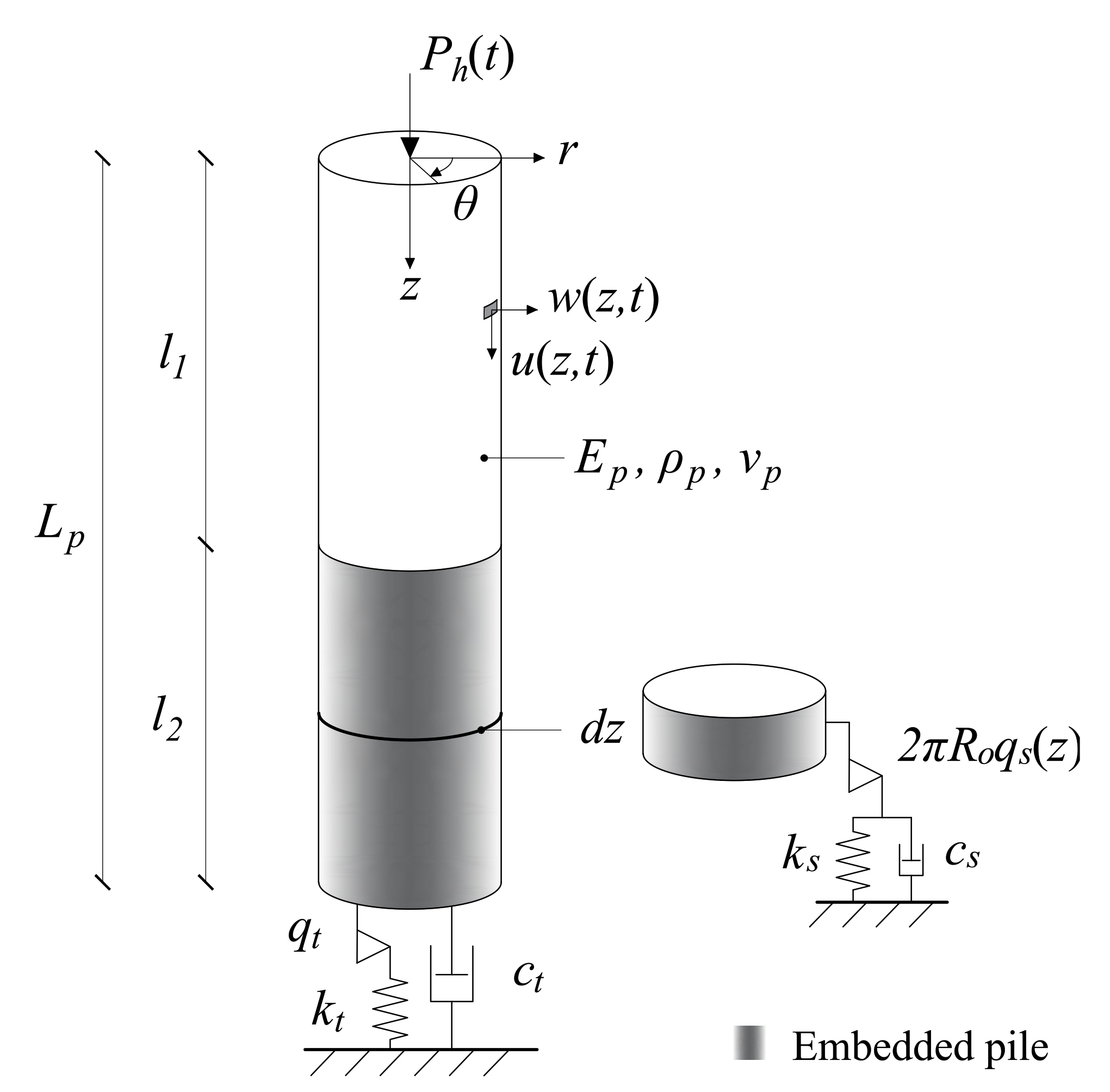
2.2. Non-Local Three-Dimensional Axisymmetric Pile Driving Model

An open-ended pipe pile, due to its cylindrical geometry, its small wall thickness compared to its other dimensions and considering the frequency range of interest, can be described as a thin cylindrical shell. In fact, the accurate description of elastic wave propagation in a pile requires a thin shell theory [26]. Notably, in the region of the frequency spectrum in which the wave dispersion is eminent, around the ring frequency of the shell $f_r$ [27], the motion of the structure is primarily radial and classical rod theory cannot capture that effect [18]. Alternative rod theories may be used, such as the Love rod theory [28] which includes dispersion, albeit it is still inaccurate in the vicinity of the ring frequency and falsely predicts a cut-off frequency. On the other hand, the thin shell theories are in excellent agreement with the results of three-dimensional elasticity theory, for the greater part of the frequency spectrum [29].

In great soil depths and thus high horizontal soil stresses, encountered during installation of monopiles in the offshore environment, the importance of accurate description of the pile motion cannot be overemphasized. Excitation of strong radial motions can affect the soil resistance during installation and render the drivability predictions inaccurate, as this effect is altogether neglected in most pile driving models. For small-diameter piles that have been mainly used offshore in the past, that issue had not arisen.

In view of the above considerations, in this work a drivability model that describes the pile by means of a thin shell theory is developed. As the pile, the force by the hammer impact, and the soil reaction, both along the shaft and at the tip, are symmetric around the pile longitudinal axis, the model used is considered axisymmetric. The latter means that all quantities of the problem are independent of the azimuth, $\theta$, i.e., ${\displaystyle \partial (·)/\partial \theta =0}$. Given the aforementioned considerations, the equations of the coupled axial-radial motion of the pile during impact driving, according to the Love-Timoshenko shell theory [30] read:

$${\displaystyle {\rho }_p{h}_p\frac{{\partial }^{2}u(z,t)}{\partial t^2}=\frac{E_p{h}_p}{\left(1-{\nu }_p^2\right)}\frac{{\partial }^{2}u(z,t)}{\partial z^2}+\frac{E_p{h}_p{\nu }_p}{\left(1-{\nu }_p^2\right)R_p}\frac{\partial w(z,t)}{\partial z}-\frac{H(z-l_1)p_s}{2\pi R_p}}$$

(7)

$${\displaystyle {\rho }_p{h}_p\frac{{\partial }^{2}w(z,t)}{\partial t^2}=-\frac{E_p{h}_p{\nu }_p}{\left(1-{\nu }_p^2\right)R_p}\frac{\partial u(z,t)}{\partial z}-\frac{E_p{h}_p}{\left(1-{\nu }_p^2\right)R_p^2}w(z,t)-\frac{E_p{h}_p^3}{12\left(1-{\nu }_p^2\right)}\frac{{\partial }^{4}w(z,t)}{\partial z^4}}$$

(8)

in which $h_p$ is the pile wall thickness and $w(z,t)$ is the radial displacement of the pile. It is remarked at this point that the soil reaction in the radial direction may also be considered, albeit in this work it is not introduced such that the two models are comparable and the effect of wave dispersion can be evaluated separately.

Similarly to Equation (3), the initial conditions are set equal to zero. For the thin cylindrical shell the axial force resultants are prescribed in the top and the bottom of the pile, while the remaining boundaries are formulated as free [31]. Accordingly, the boundary conditions read:

$$\begin{array}{c}\hfill {\displaystyle N_z(0,t)=-\frac{P_h\left(t\right)}{2\pi R_p},N_{z\theta }(0,t)=0,Q_z(0,t)=0,M_z(0,t)=0,}\\ \hfill {\displaystyle N_z(L_p,t)=-\frac{P_t}{2\pi R_p},N_{z\theta }(L_p,t)=0,Q_z(L_p,t)=0,M_z(L_p,t)=0}\end{array}$$

(9)

in which $N_z(z,t)$, $N_{z\theta }(z,t)$ and $Q_z(z,t)$ denote the axial, in-plane shear and out-plane shear force resultants, respectively, and $M_z(z,t)$ denotes the moment resultant of the thin cylindrical shell [26]. The natural boundary conditions from Equation (3) have been reformulated into Equation (9), such that the prescribed forces at the boundaries, $P_h\left(t\right)$ and $P_t$, are uniformly distributed along the pile circumference. Finally, the ultimate shaft and tip resistances are identical to the ones described in Section 2.1 and the described model is displayed in Figure 2.

As stated before, one of the main challenges in pile drivability predictions, lies in the strong need for a simple and accurate description of the soil reaction. Available models employ local and frequency-independent springs and dashpots, arranged together with non-linear elements to account for the soil reaction in a computationally efficient manner. The significance of the accuracy in the modelling of the linear part of these phenomenological models is enhanced when a pile is close to refusal during driving and essentially the linear regime is strongly present [32]. In view of the aforementioned, the employment of non-local elasticity comprises a significant step towards computationally efficient and more realistic foundation models [33], while it has been recently applied for capturing the lateral response of monopiles [34].

In the present study, the approach adopted is similar to Friswell [33]. It is assumed that the spatial kernel function is a Gaussian function $g(z,\xi )$, normalized as shown in [35], with the following form:

$${\displaystyle g(z,\xi )=\frac{\alpha }{\sqrt{2\pi }}{\mathrm{e}}^{-\frac{{\alpha }^2{(z-\xi )}^2}{2}}}$$

(10)

in which $\alpha$ is the inverse of the influence distance of the spatial kernel function $g(z,\xi )$ (see Figure 3). At this point let us remark that the local foundation models can also be described in this form and essentially comprise a special sub-category with spatial kernel function equal to the Dirac delta function, $g(z,\xi )=\delta (z-\xi )$. The latter means that the foundation is locally reacting. According to the previous, the non-local soil reaction along the pile shaft, ${\tilde{p}}_s$, reads:

$${\tilde{p}}_s=\left\{\begin{array}{cc}{\displaystyle \underset{l_1}{\overset{L_p}{\int }}g(z,\xi )\left(k_s\left(u(\xi ,t)-u_{eq,s}(\xi ,t)\right)+c_s\frac{\partial u(\xi ,t)}{\partial t}\right)d\xi =G(z,t),}\hfill & {\displaystyle \mathrm{for}\left|G(z,t)\right|\le 2\pi R_o{q}_s}\hfill \\ {\displaystyle 2\pi R_o{q}_{s}sgn\left(\frac{\partial u(z,t)}{\partial t}\right),}\hfill & {\displaystyle \mathrm{for}\left|G(z,t)\right|>2\pi R_o{q}_s}\hfill \end{array}\right.$$

(11)

The present non-local soil reaction model comprises an extension of its local counterpart, by coupling of the locally reacting elements through prescribed spatial kernel functions. The accuracy of such models can be evaluated properly, only by comparison with the dynamic reaction of the three-dimensional soil continuum, which is not considered in this work.

2.3. Numerical Solution

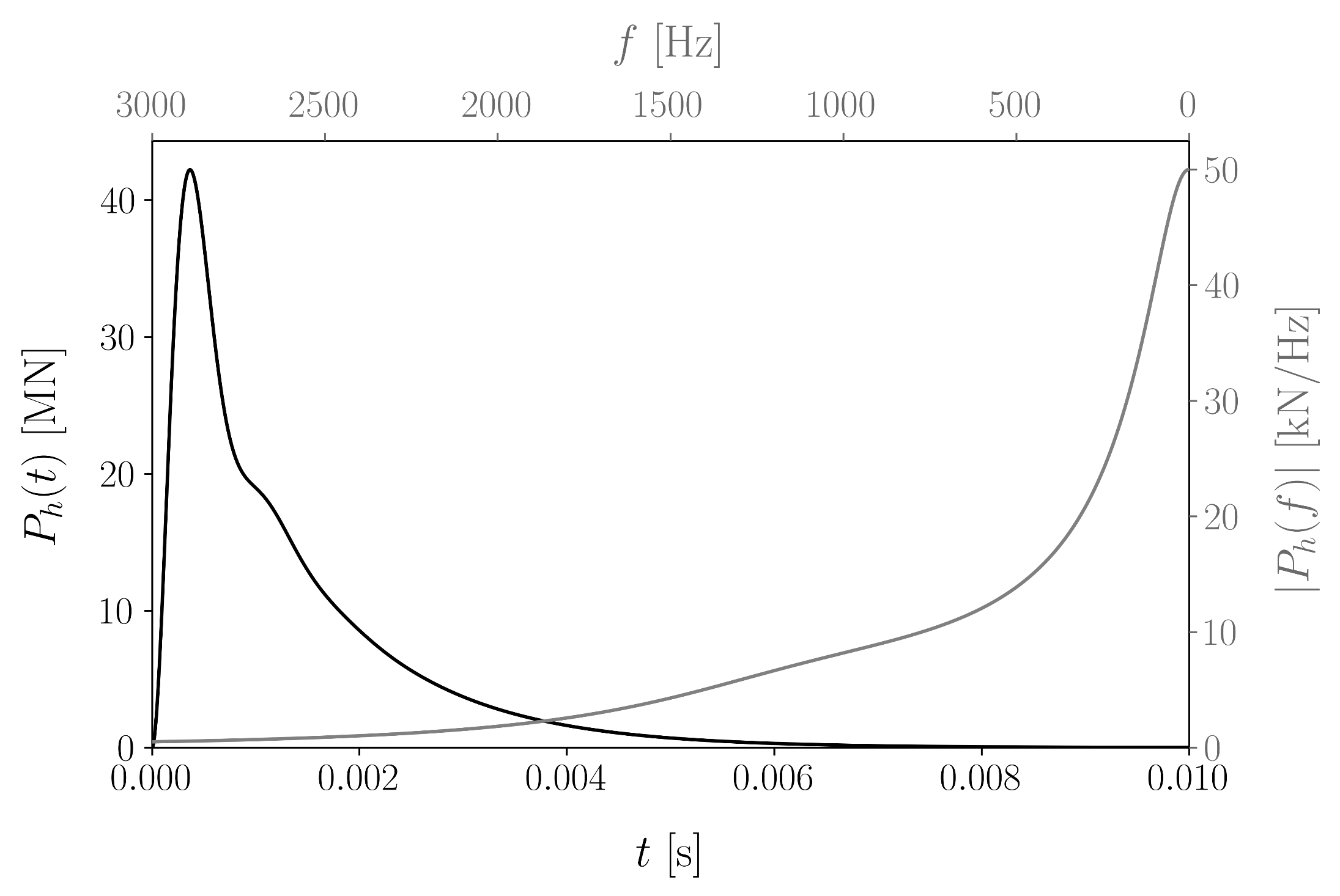
For the one-dimensional model presented in Section 2.1, henceforth called 1-d FD model for brevity, the method of central finite differences, of accuracy $\mathcal{O}(\Delta z^2)$, is employed for the spatial discretization. The boundary conditions are treated by introducing fictitious nodes [36] and the non-linear partial differential equation (PDE) governing the pile motion, is decomposed into a set of non-linear ordinary differential equations (ODEs) representing the dynamic equilibria of the pile nodes.

On the contrary, for the three-dimensional axisymmetric model, henceforth referred to as 3-d LT model for brevity, the Galerkin method is employed for the spatial discretization of the thin cylindrical shell [37]. A series discretization method is advantageous for this system, compared to a method such as finite differences that leads to ODEs at nodal points and thus increases the computational complexity, due to the dimensions of the problem. The Galerkin method circumvents the problem of dimensions, albeit requires a more laborious analytical treatment to utilize its benefits in our case. First, the reformulation of the boundary conditions is performed, as we have a time-dependent boundary condition at $z=0$ and a non-linear boundary condition at $z=L_p$. The concentrated body force method (CBFM) is used to reformulate the boundary conditions into stress-free boundaries and to translate the boundary stresses into the equation of motion by means of the Dirac delta function $\delta (·)$ [38]. At this point, the free vibration modes of the free-free cylindrical shell in vacuo are found and employed in our solution as trial and test functions. The solution to the free vibration problem can be written in the form:

$${\displaystyle u=\sum _{m=0}^{\infty }{U}_m\left(z\right){\mathrm{e}}^{i{\omega }_{m}t},w=\sum _{m=0}^{\infty }{W}_m\left(z\right){\mathrm{e}}^{i{\omega }_{m}t}}$$

(12)

with $U_m\left(z\right)$ and $W_m\left(z\right)$ being the modal displacements of the m-th free vibration mode in the axial and radial directions, respectively, and ${\omega }_m$ denoting the m-th natural frequency. Therefore, the solution of Equations (7) and (8) is approximated by the series:

$${\displaystyle u=\sum _{m=0}^{N_m}{U}_m\left(z\right)q_m\left(t\right),w=\sum _{m=0}^{N_m}{W}_m\left(z\right)q_m\left(t\right)}$$

(13)

in which $q_m\left(t\right)$ is the m-th generalized coordinate and $N_m$ is the upper limit of the truncated summation, adequate to provide a sufficiently accurate solution. By substituting Equation (13) into Equations (7) and (8) the residual is obtained and by integrating over the shell domain the product of each test function with the residual, the weighted residual, is derived. By setting the latter equal to zero a set of $N_m$ non-linear coupled ODEs of $q_m\left(t\right)$ is formulated. Conclusively, for both 1-d FD and 3-d LT models the resulting sets of ODEs are arranged in the state-space form, in order to facilitate numerical integration. The explicit Runge-Kutta method of accuracy $\mathcal{O}(\Delta t^4)$ is used in both cases [39].

For both models, the frequency with amplitude equal to the 10% of the maximum force amplitude (see Section 3.2) and the corresponding wavelength are used to determine the discretization parameters. For the 1-d FD model the time step is defined as $\Delta t=\Delta z/\left(10c_p\right)$, in which $\Delta z$ denotes the spatial mesh size, equal to the smallest wavelength to be analysed, and $c_p$ is the longitudinal wave velocity in the pile, such that 10 time steps are used to represent the wave with the shortest wavelength [40]. In the 3-d LT model, the upper frequency limit is used to select the truncation limit $N_m$ in Equation (13) and the time step is set equal to $\Delta t=\pi /\left(5{\omega }_m\right)$ (10 time steps for the highest frequency component ${\omega }_m$). Further refinement of the previous discretization parameters is performed until convergence is met, defined as:

$${\displaystyle {ϵ}_i=\frac{\left|u_{i+1}(z,t)-u_i(z,t)\right|}{\left|u_{i+1}(z,t)\right|}<1\%}$$

(14)

in which ${ϵ}_i$ is the relative error of the displacement field between the i-th and $(i+1)$-th analyses, used as the convergence criterion.

3. Results

In Section 3.1 the validity of the 3-d LT model is verified, by reducing it into a physically equivalent model to 1-d FD, for direct comparison. Furthermore, in Section 3.2 and Section 3.3 numerical examples that consider the influence of wave dispersion and non-local soil reaction, respectively, are presented.

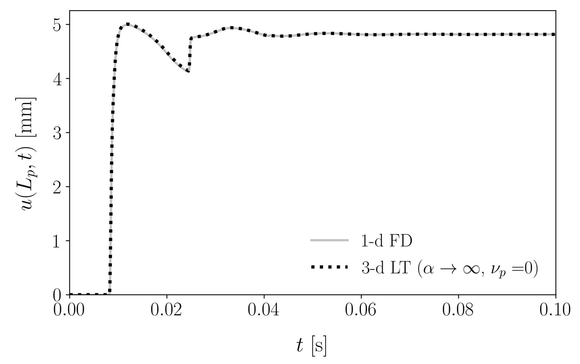
3.1. Validation of the 3-d LT Model

At first, a set of numerical analyses for a single hammer blow are performed to showcase the validity of the 3-d LT model. For this purpose, the 1-d FD model formulated in Section 2.1 is used as reference and its results are compared to the respective ones obtained from the 3-d LT model, upon proper reduction to an equivalent classical rod with local soil reaction. By setting the Poisson’s ratio of the pile ${\nu }_p=0$ and discarding Equation (8), the Love-Timoshenko shell theory is reduced to the classical rod theory. Furthermore, by considering $\alpha \to \infty$, the spatial kernel becomes $g(z,\xi )=\delta (x-\xi )$ and the soil reaction is rendered local. Under these considerations, the pile is equivalently described by the classical rod theory and the soil reaction is local, in both models. In view of the previous, the results of the numerical analyses by 1-d FD and reduced 3-d LT should be identical.

The parameters of the validation case are shown in

Table 1. Parameters of the validation case.

Pile	Young’s modulus	$E_p$	210 GPa
	Mass density	${\rho }_p$	7850 kg/m${}^3$
	Poisson’s ratio	${\nu }_p$	0.3
	Length	$L_p$	42 m
	Radius	$R_p$	1.1 m
	Wall thickness	$h_p$	0.03 m
	Initial embedment depth	$l_2$	25.2 m
Soil	Shear modulus	$G_s$	18.52 MPa
	Mass density	${\rho }_s$	1900 kg/m${}^3$
	Poisson’s ratio	${\nu }_s$	0.35
	Friction angle	${\varphi }^{\prime }$	35${}^{\circ }$
	Soil-pile interface friction angle	${\delta }^{\prime }$	31.5${}^{\circ }$
Hammer	Ram mass	$m_r$	10,000 kg
	Anvil mass	$m_a$	1000 kg
	Cushion stiffness	$k_c$	70.87 × ${10}^6$ kN/m
	Ram impact velocity	$v_0$	5 m/s

and the hammer force function, $P_h\left(t\right)$, together with the amplitude of its Fourier transform, $|P_h\left(f\right)|$, are depicted in Figure 4.

In Figure 5 the axial tip displacement, $u(L_p,t)$, is presented for a single hammer blow, as obtained by the two models in consideration. Evidently, the response obtained by the two approaches is in excellent agreement. Therefore, in the following analyses the capabilities of the 3-d LT model can be utilized fully, to study the two mechanisms under discussion in this work, namely the dispersion of elastic waves in the pile and the introduction of non-locality in the soil reaction along the pile shaft.

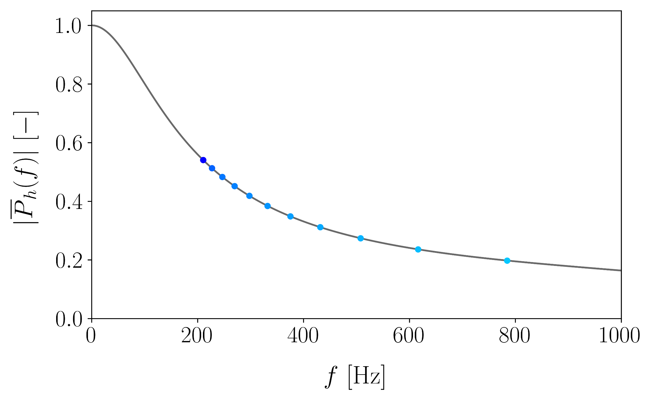
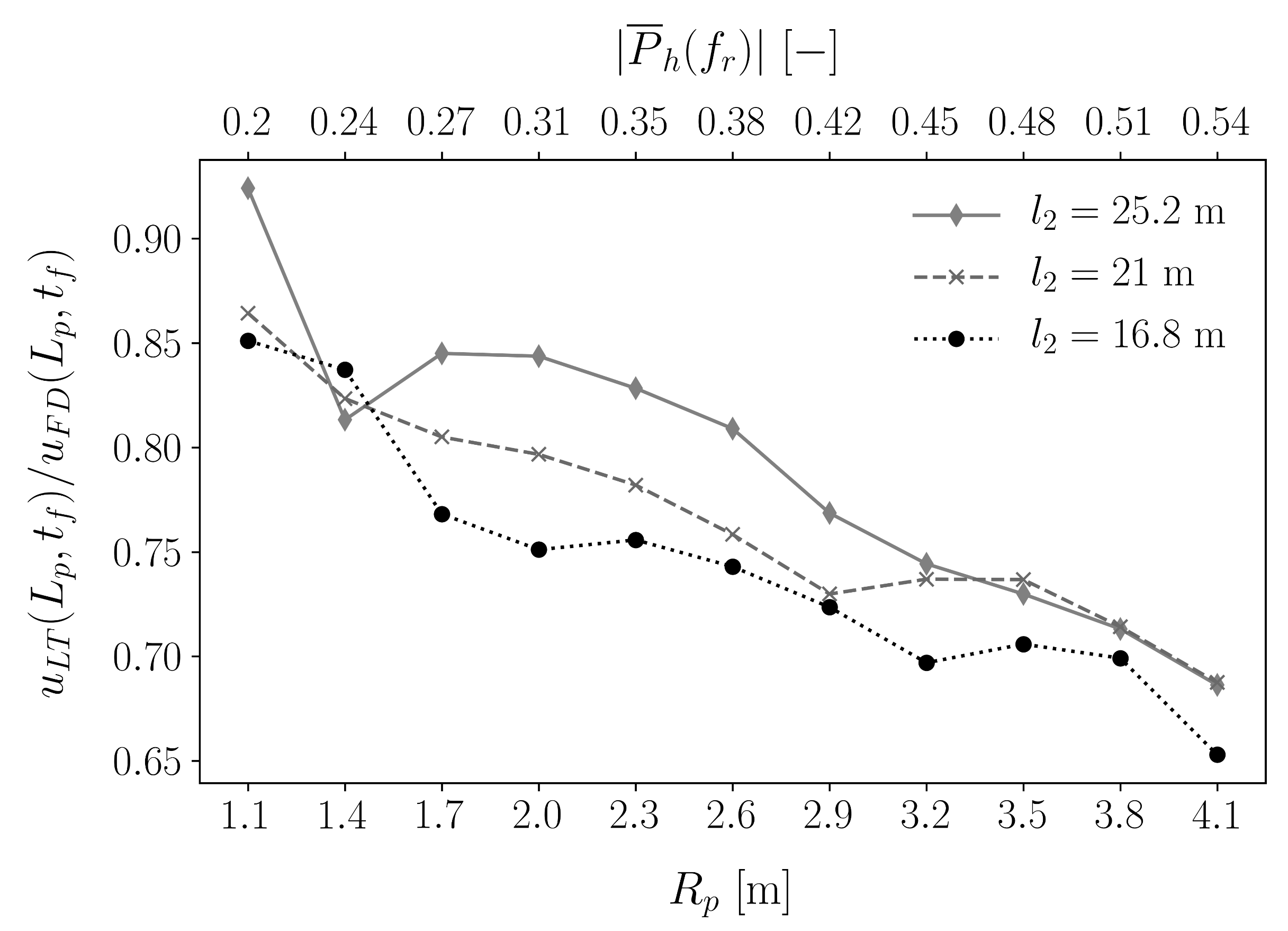
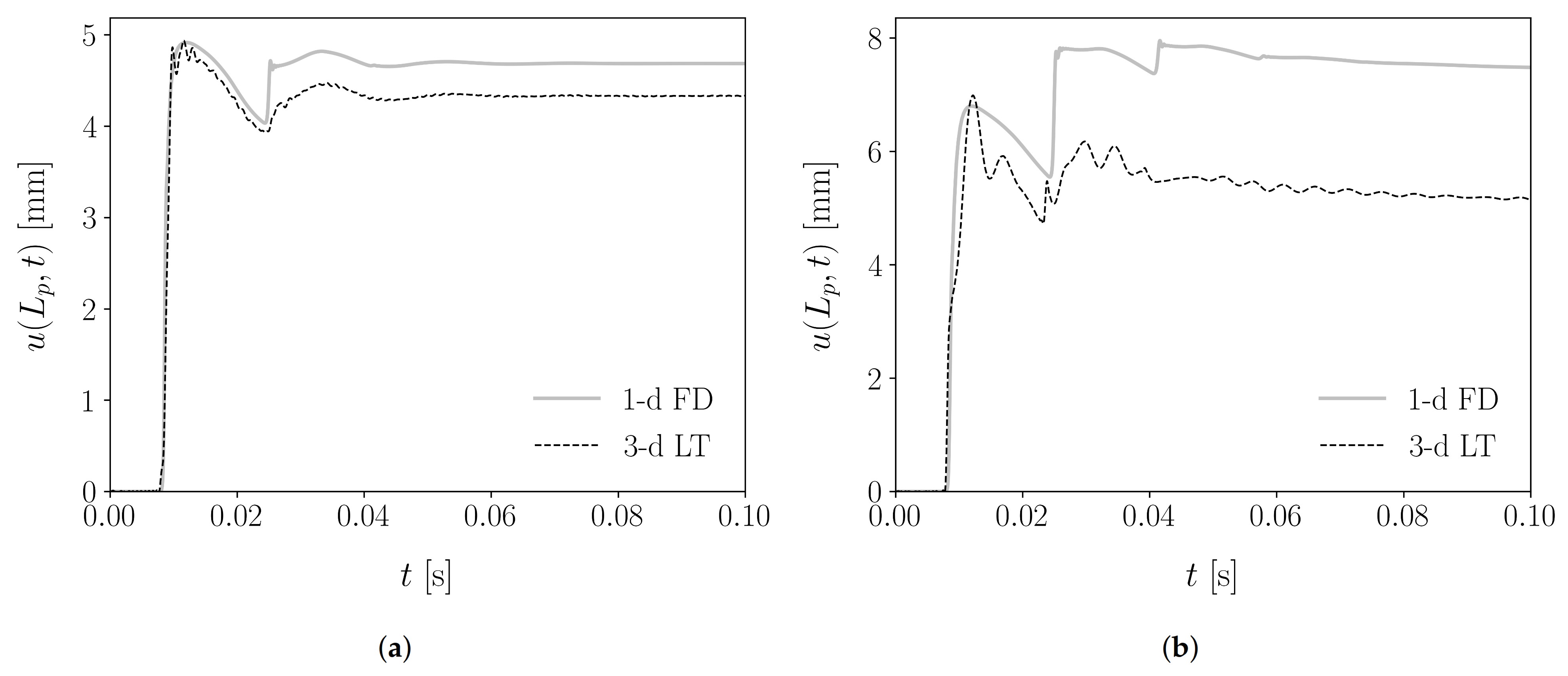
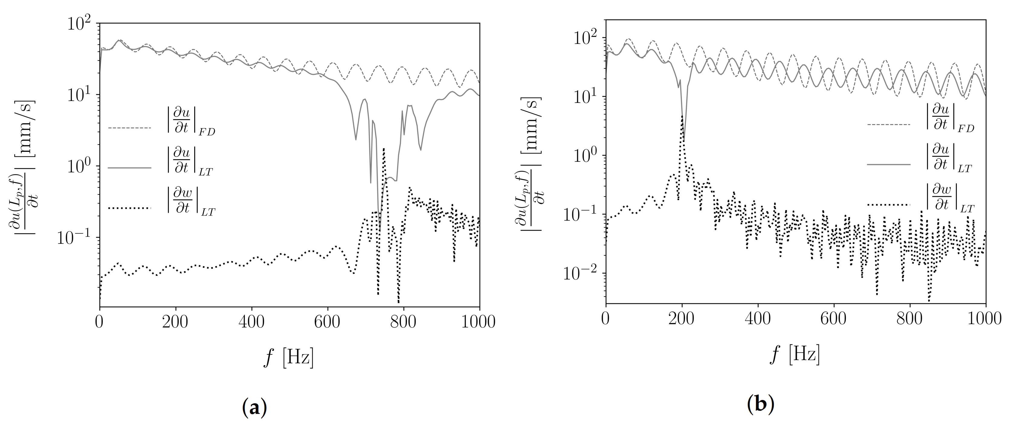
3.2. Influence of Wave Dispersion

To isolate the effect of wave dispersion, the 3-d LT model used in the following examples, had local soil reaction and differed from the 1-d FD solely in the pile description as a thin cylindrical shell. For the following numerical examples, all the parameters had the values given in Table 1, except for $R_p$, $h_p$, $l_2$ and the hammer parameters. The initial embedment depths of $l_2=0.4L_p,0.5L_p,0.6L_p$ were considered, while various pile radii, $R_p$, were used in the analyses (see

Table 2. Set of variable pile parameters.

$R_p$	1.1 m	1.4 m	1.7 m	2.0 m	2.3 m	2.6 m	2.9 m	3.2 m	3.5 m	3.8 m	4.1 m
$h_p$	0.03 m	0.03 m	0.03 m	0.04 m	0.04 m	0.04 m	0.04 m	0.05 m	0.05 m	0.05 m	0.05 m

), to identify the effect of these parameters on the wave dispersion. In Table 2 each column provides a pair of pile radius, $R_p$, and wall thickness, $h_p$, leading to eleven different pile geometries.

Regarding the properties of the hammer, attention was needed in order to have results that can be compared on a rational basis. For that purpose, normalization of the hammer force was performed for all pile driving cases, such that the maximum axial stress at the pile head was equal to 57% of the yield stress, $f_y=355$ MPa. The dimensionless mass ratio, $m_a\ast =m_a/m_r$, and the dimensionless cushion stiffness, $k_c^{*}=k_c{m}_r/Z_p^2$, with $Z_p$ denoting the pile impedance, were used in order to achieve the normalization in all cases [22]. The aforementioned parameters were set to $m_a\ast =0.1$ and $k_c^{*}=10$ in all the cases studied, while the ram impact velocity, $v_0$, was equal to 5 m/s. Therefore, depending on the pile geometry, the values of ram mass, $m_r$, anvil mass, $m_a$, and cushion stiffness, $k_c$, were scaled in order to preserve the dimensionless quantities and the maximum axial stress level constant. According to the previous, the Fourier transform of the hammer force, normalized over the maximum amplitude at zero frequency as $|{\overline{P}}_h\left(f\right)|=|P_h\left(f\right)|/|P_h\left(0\right)|$, is identical for all piles considered. In Figure 6 the normalized amplitude of the hammer force spectrum is depicted together with the normalized amplitude at the ring frequency of each pile of this study, indicated by the blue markers.

In Figure 7 the ultimate pile set ratio $u_{LT}(L_p,t_f)/u_{FD}(L_p,t_f)$ is displayed, in which $u_{LT}(L_p,t_f)$ and $u_{FD}(L_p,t_f)$ denote the tip displacement of 3-d LT and 1-d FD, respectively, at the final time moment of the analysis, $t_f$. It is noted that $t_f$ was adequate for the imparted energy into the pile to dissipate through the soil reaction and the final set to be obtained. As can be observed, for all the examined pile radii and embedment depths there is deviation from the dispersionless response (i.e., ratio equal to 1.0) of the 1-d FD model. Consequently, wave dispersion does have an effect even for small-diameter piles, albeit its influence on the final pile set is not as high as in the large-diameter cases. With ascending radius $R_p$, the amount of energy imparted in frequencies around the ring frequency $f_r$ becomes significant. As a result the increase of $|{\overline{P}}_h\left(f_r\right)|$ leads clearly to reduction of the ultimate set ratio, as direct consequence of dispersion effects. Embedment depth, $l_2$, seems to be beneficial for the ultimate set ratio and mitigate partially these effects, which is rational since additional damping is provided from the increased length of the shaft in contact with the soil. The motions that are responsible for the wave dispersion are high-frequency motions, thus increased embedment depth contributes into their decay and results in a weaker influence on the pile response overall. Notwithstanding the remarks about embedment depth, it seems that for large radii ($R_p\ge 3.0$ m), or better for high $|{\overline{P}}_h\left(f_r\right)|$, the set ratio is less sensitive to its influence. For these pile geometries the ring frequency, $f_r$, corresponds to frequencies that are significantly excited by the hammer impact as $|{\overline{P}}_h\left(f_r\right)|$ approaches 0.5 and relevant induced pile motions obtain large amplitudes. The aforementioned observations and relevant remarks are better understood through Figure 8 and Figure 9.

The tip displacement obtained by the two considered models, for the extreme scenarios of the smallest and the largest pile radii, are shown in Figure 8. Evidently, the two responses for $R_p=4.1$ m (Figure 8b) deviate much more than for $R_p=1.1$ m (Figure 8a). In Figure 8a, the displacement mainly diverges for the two approaches after the second arrival of the impact-induced stress wave at the pile tip (after $t=0.02$ s), but follows the same trend. On the contrary, in Figure 8b the response becomes dissimilar already after the first arrival of the stress wave at the pile tip, as the frequency content of this motion is much richer in components that display dispersive behaviour. The discrete Fourier transform (DFT) spectra of the velocities for the cases analysed in Figure 8, are given in Figure 9 to supplement the previous statement.

In Figure 9a the amplitude of the axial velocity spectrum for both models is in good agreement approximately up to 600 Hz. At that point the amplitude of the axial velocity in the 3-d LT model drops significantly and energy in axial motion is reduced at these frequencies. However, it is not the case that energy is not present in this region of the frequency spectrum in the pile motion. As can be observed, the radial velocity amplitudes surge in this region of the spectrum and even surpass the amplitudes of the axial velocity in some frequencies. For this case the ring frequency is $f_r$ = 784.48 Hz, which supports our findings. Considering further the case of $R_p=4.1$ m, in Figure 9b the velocity spectrum shows some differences with respect to Figure 9a. First, the drop corresponding to the vicinity of the ring frequency occurs much lower in the frequency axis, as $f_r$ = 210.47 Hz and even for the first small peaks in axial velocity, discrepancy exists between the two models. The latter already indicates that dispersion is present in lower frequency components than in Figure 9a, in which energy imparted from the hammer impact is greater (see Figure 6). The peaks that can be distinguished in both Figure 9a,b correspond to the natural frequencies of free vibration of the pile in vacuo, which are correctly represented by the 3-d LT model as has been discussed in Section 2.2. For $R_p=1.1$ m, the velocity amplitudes are in good agreement up to certain frequency (approximately 600 Hz), albeit for $R_p=4.1$ m they clearly deviate along the whole spectrum indicating the inaccurate description of wave propagation in the 1-d FD model. The aforementioned remarks lead to the discrepancy observed in Figure 8b.

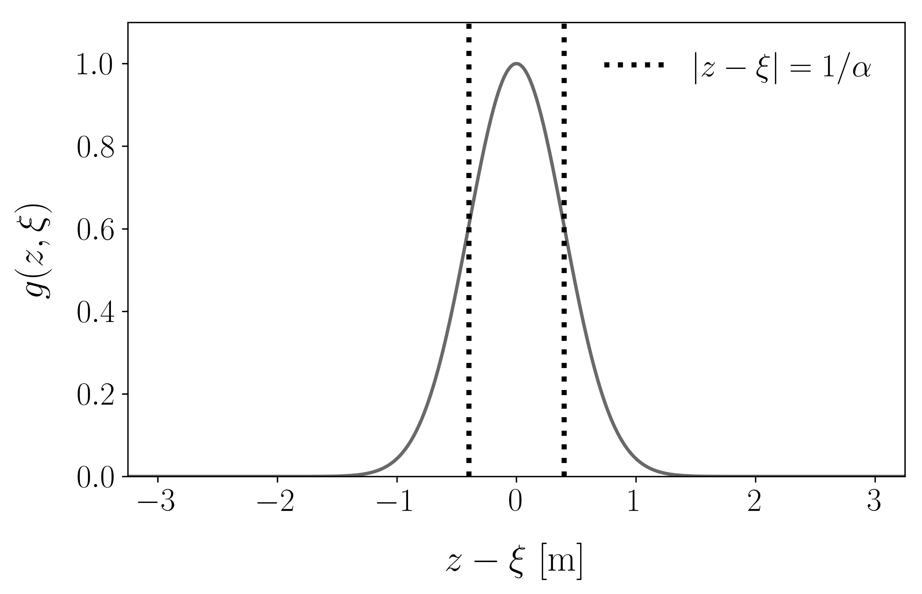
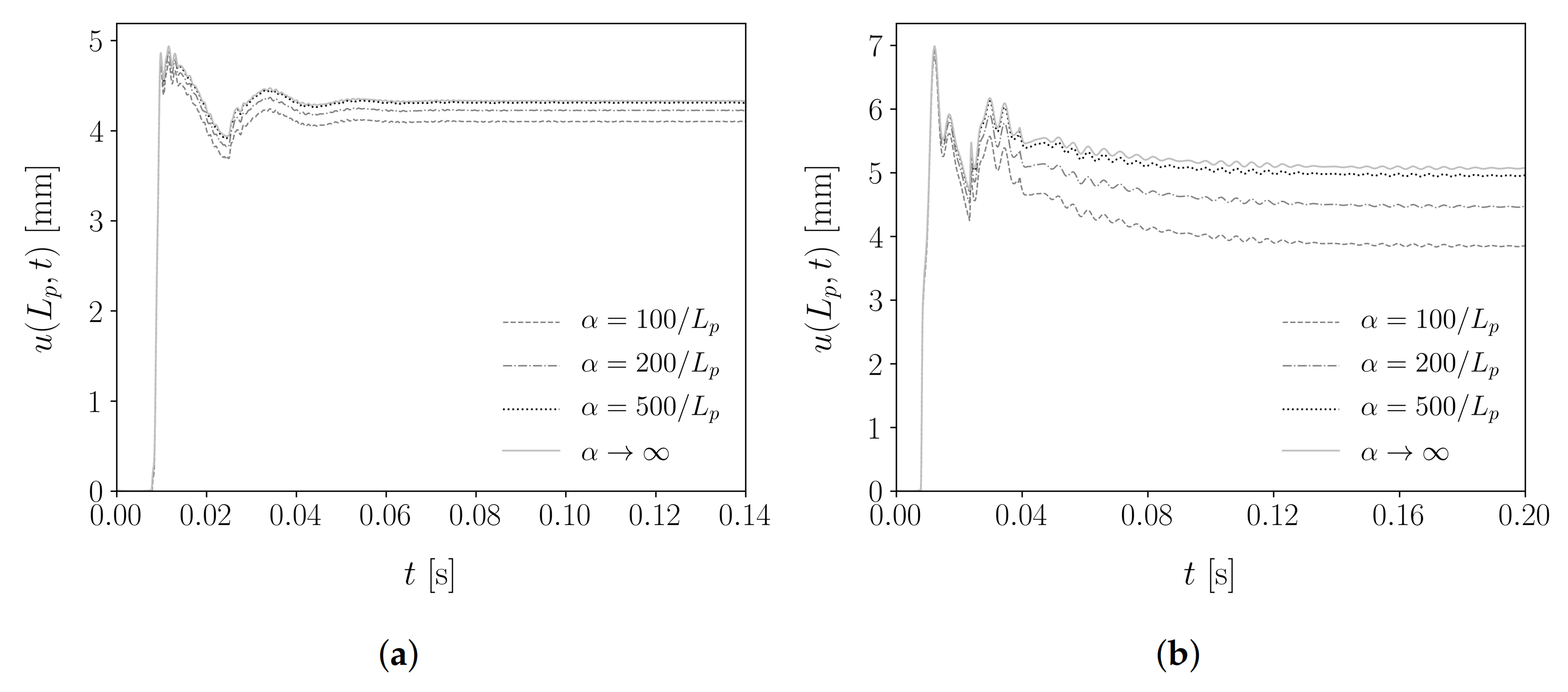
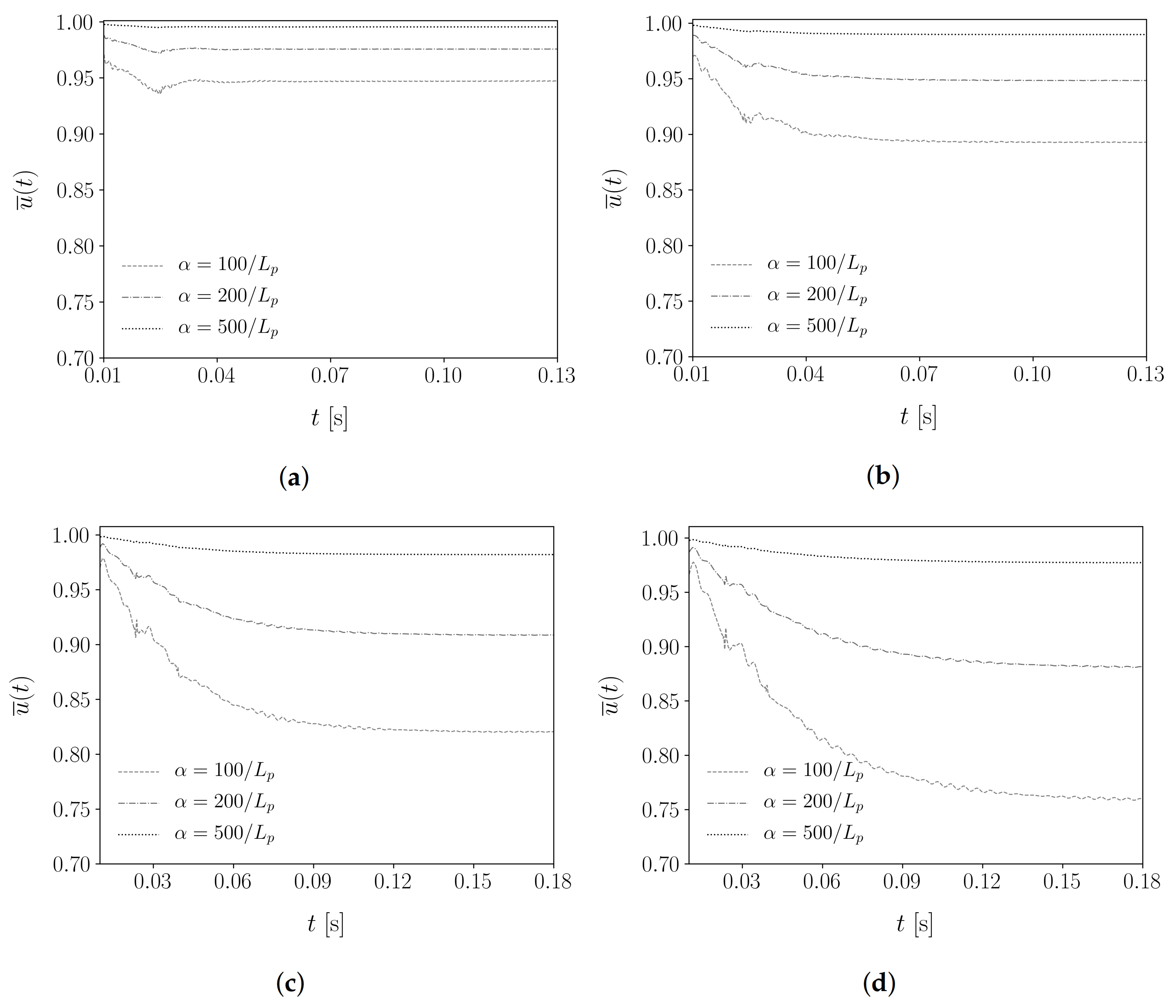
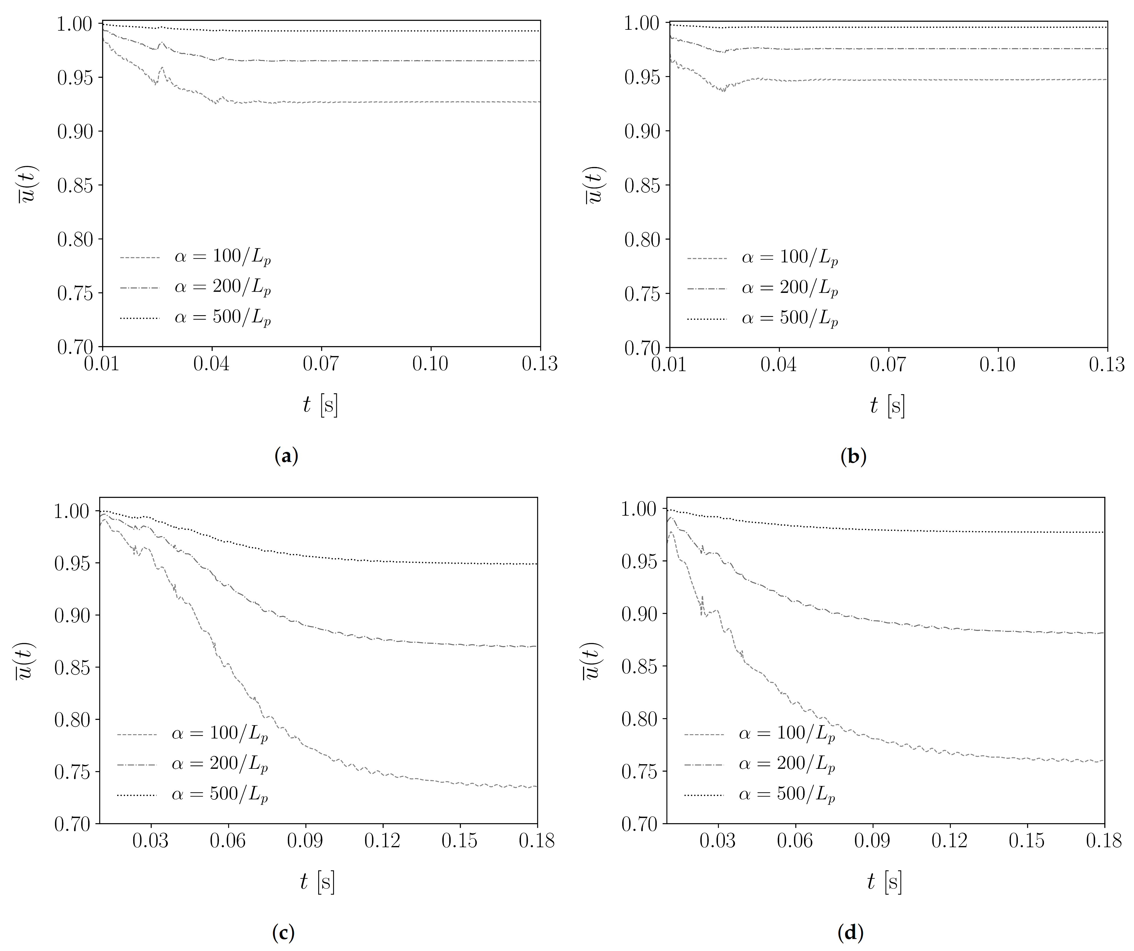
3.3. Influence of Non-Local Soil Reaction

At this point, the introduction of non-locality in the soil reaction of the 3-d LT model is examined. For that purpose, the 3-d LT with local soil reaction and its non-local counterpart are compared. The exact spatial distribution of the non-local soil reaction is not known and in this work the Gaussian function is assumed as the spatial kernel a priori, with three different values of influence distance considered, namely $1/\alpha =L_p/100,L_p/200,L_p/500$. In Figure 10 the axial tip displacement, $u(L_p,t)$, is presented for $R_p=1.1$ m and $R_p=4.1$ m ($l_2=25.2$ m). As can be seen, the divergence of the displacement obtained by the non-local models compared to the local one is much stronger for the large-diameter pile.

To better evaluate the effects of non-locality, in Figure 11 for each pile the displacement ratio of non-local to local models, ${\displaystyle \overline{u}\left(t\right)=u(L_p,t)/{\left.u(L_p,t)\right|}_{\alpha \to \infty }}$ is examined for four different pile radii. The effect of non-locality seems to become more eminent for large-diameter piles and the deviation even between the non-local models for different values of $\alpha$ becomes quite important. On the other hand, for $R_p=1.1$ m and $R_p=2.0$ m.

All the non-local reaction models considered present a ratio, $\overline{u}\left(t\right)$, from 0.9 to 1.0, practically meaning that for the values of $\alpha$ considered, local and non-local reaction do not significantly alter the final pile penetration. In all cases, the non-locality seems to reduce the final pile penetration for the considered soil profile. Furthermore, the increase of $\alpha$ (decrease of influence distance) tends to provide a response that converges to the one of the local reaction model, which is rational. To summarize, Figure 11 reveals that the non-locality of soil reaction can affect the pile response in variable degree and the pile radius seems to be a significant factor that determines the amount of this influence.

Apart from the pile radius, the parameter of the embedment depth $l_2$, is finally considered. In Figure 12, the smallest ($R_p=1.1$ m) and the largest ($R_p=4.1$ m) pile radii of this study are shown, for $l_2=16.8$ m and $l_2=25.2$ m. At a first glance, the different values of $l_2$ do not appear to significantly alter the displacement ratios, $\overline{u}\left(t\right)$. For both piles the larger $l_2$ value seems to lead to a minor reduction of $\overline{u}\left(t\right)$. Finally, the introduction of the soil reaction in the radial direction and its effect on the pile penetration comprises an additional step, not considered herein as this work focuses on dispersive wave propagation and non-local soil reaction in the direction of driving.

4. Conclusions

In this paper a three-dimensional axisymmetric pile driving model with non-local soil reaction is developed. The pile description is based on the Love-Tismohenko theory for thin cylindrical shells and the non-local soil reaction is formulated as a convolution integral of local soil reaction models and the Gaussian function as spatial kernel. Furthermore, a one-dimensional model, according to widely adopted approaches in the area of pile driving, is formulated and used for comparison, in order to investigate the effects of dispersion of elastic waves and non-locality of soil reaction.

First, the dispersion of elastic waves in the pile was studied, for various pile geometries and initial embedment depths. The main argument of the significance of wave dispersion in drivability of large-diameter monopiles was ascertained, as the effect of dispersion was found to increase with ascending pile radius. Embedment depth provided some mitigation of this effect for small-to-medium pile radii, while for large-diameter piles the effect of wave dispersion was sustained even for large pile embedments. In the vicinity of the ring frequency pile motion is predominantly radial and significantly excited by the hammer impact for large-diameter monopiles. This effect cannot be captured by one-dimensional models and can alter the soil resistance to driving. In the current effort to modify, or even reinvent, the existing drivability approaches for large-diameter monopiles the proper description of the pile motion is essential. Otherwise, certain response features in monopile installation data, resulting from wave dispersion, may be falsely attributed to other mechanisms, e.g., soil non-linear behaviour, and lead us further away from an accurate approach to predict monopile drivability.

Conclusively, the introduction of non-local soil reaction has been realized. A system of integro-differential equations is obtained, which is solved by means of the Galerkin method and numerical integration. The results from this study are mostly an indication of how non-local reaction can affect the pile penetration during impact piling. The effect of non-locality was found to be more influential in the case of large diameters, while the variable embedment depth yielded minor differences between local and non-local models. Decrease of the influence distance, $1/\alpha$, showcased the trend to converge to the response of the local reaction model, which is the expected behaviour. Results for various influence distances comprise an indication of the degree to which non-locality may or may not affect the overall behaviour. Finally, the refinement of the non-local soil reaction by introducing a frequency-dependent spatio-temporal kernel, based on the response of the three-dimensional soil continuum is considered the optimal next step for the development of the present model.

References

1. Poudineh, R.; Brown, C.; Foley, B. Economics of Offshore Wind Power: Challenges and Policy Considerations; Springer: Berlin/Heidelberg, Germany, 2017. [Google Scholar]
2. Sánchez, S.; López-Gutiérrez, J.S.; Negro, V.; Esteban, M.D. Foundations in offshore wind farms: Evolution, characteristics and range of use. Analysis of main dimensional parameters in monopile foundations. J. Mar. Sci. Eng. 2019, 7, 441. [Google Scholar] [CrossRef] [Green Version]
3. Asgarpour, M. Assembly, transportation, installation and commissioning of offshore wind farms. In Offshore Wind Farms; Elsevier: Amsterdam, The Netherlands, 2016; pp. 527–541. [Google Scholar]
4. Wu, X.; Hu, Y.; Li, Y.; Yang, J.; Duan, L.; Wang, T.; Adcock, T.; Jiang, Z.; Gao, Z.; Lin, Z.; et al. Foundations of offshore wind turbines: A review. Renew. Sustain. Energy Rev. 2019, 104, 379–393. [Google Scholar] [CrossRef] [Green Version]
5. Sa, L.; Yinghui, T.; Yangrui, Z.; Baofan, J.; Jinbiao, W. Premature refusal of large-diameter, deep-penetration piles on an offshore platform. Appl. Ocean Res. 2013, 42, 55–59. [Google Scholar] [CrossRef]
6. Ramírez, L.; Fraile, D.; Brindley, G. Offshore Wind in Europe: Key Trends and Statistics 2019; Technical Report; WindEurope: Brussels, Belgium, 2020. [Google Scholar]
7. Gerwick, B.C., Jr. Construction of Marine and Offshore Structures; CRC Press: Boca Raton, FL, USA, 2007. [Google Scholar]
8. Smith, E.A. Pile-driving analysis by the wave equation. Am. Soc. Civ. Eng. Trans. 1962, 127, 1145–1170. [Google Scholar] [CrossRef]
9. Randolph, M.F.; Simons, H.A. An improved soil model for one-dimensional pile driving analysis. In Proceedings of the 3rd International Conference on Numerical Methods in Offshore Piling, Nantes, France, 21–22 May 1986; pp. 1–17. [Google Scholar]
10. Lee, S.; Chow, Y.; Karunaratne, G.; Wong, K. Rational wave equation model for pile-driving analysis. J. Geotech. Eng. 1988, 114, 306–325. [Google Scholar] [CrossRef]
11. Novak, M. Vertical vibration of floating piles. J. Eng. Mech. Div. 1977, 103, 153–168. [Google Scholar] [CrossRef]
12. Novak, M.; Aboul-Ella, F.; Nogami, T. Dynamic soil reactions for plane strain case. J. Eng. Mech. Div. 1978, 104, 953–959. [Google Scholar] [CrossRef]
13. Byrne, T.; Doherty, P.; Gavin, K.; Overy, R. Comparison of pile driveability methods in North Sea sand. In Offshore Site Investigation and Geotechnics: Integrated Technologies-Present and Future; Society of Underwater Technology: London, UK, 2012. [Google Scholar]
14. Anusic, I.; Eiksund, G.R.; Liingaard, M.A. Comparison of pile driveability methods based on a case study from an offshore wind farm in North Sea. In Proceedings of the 17th Nordic Geotechnical Meeting Challenges in Nordic Geotechnic, Reykjavik, Iceland, 25–28 May 2016. [Google Scholar]
15. Byrne, T.; Gavin, K.; Prendergast, L.; Cachim, P.; Doherty, P.; Pulukul, S.C. Performance of CPT-based methods to assess monopile driveability in North Sea sands. Ocean Eng. 2018, 166, 76–91. [Google Scholar] [CrossRef] [Green Version]
16. Deng, Q.; Jiang, W.; Zhang, W. Theoretical investigation of the effects of the cushion on reducing underwater noise from offshore pile driving. J. Acoust. Soc. Am. 2016, 140, 2780–2793. [Google Scholar] [CrossRef]
17. Meijers, P.; Tsouvalas, A.; Metrikine, A. The effect of stress wave dispersion on the drivability analysis of Large-Diameter monopiles. Procedia Eng. 2017, 199, 2390–2395. [Google Scholar] [CrossRef]
18. Paliwal, D.; Pandey, R.K.; Nath, T. Free vibrations of circular cylindrical shell on Winkler and Pasternak foundations. Int. J. Press. Vessel. Pip. 1996, 69, 79–89. [Google Scholar] [CrossRef]
19. De Nicola, A.; Randolph, M.F. Tensile and compressive shaft capacity of piles in sand. J. Geotech. Eng. 1993, 119, 1952–1973. [Google Scholar] [CrossRef]
20. Deeks, A.J.; Randolph, M.F. Axisymmetric time-domain transmitting boundaries. J. Eng. Mech. 1994, 120, 25–42. [Google Scholar] [CrossRef]
21. Liyanapathirana, D.; Deeks, A.; Randolph, M. Numerical analysis of soil plug behaviour inside open-ended piles during driving. Int. J. Numer. Anal. Methods Geomech. 1998, 22, 303–322. [Google Scholar] [CrossRef]
22. Deeks, A.; Randolph, M. Analytical modelling of hammer impact for pile driving. Int. J. Numer. Anal. Methods Geomech. 1993, 17, 279–302. [Google Scholar] [CrossRef]
23. Egorov, K. Calculation of bed for foundation with ring footing. In Proceedings of the 6th International Conference of Soil Mechanics and Foundation Engineering, Montreal, QC, Canada, 8–15 September 1965; Volume 2, pp. 41–45. [Google Scholar]
24. Poulos, H.G.; Davis, E.H. Pile Foundation Analysis and Design; Number Monograph; Wiley: Hoboken, NJ, USA, 1980. [Google Scholar]
25. Kumar, J.; Chakraborty, M. Bearing capacity factors for ring foundations. J. Geotech. Geoenviron. Eng. 2015, 141, 06015007. [Google Scholar] [CrossRef]
26. Leissa, A.W. Vibration of Shells; Scientific and Technical Information Office, National Aeronautics and Space Administration: Hampton, VA, USA, 1973; Volume 288. [Google Scholar]
27. Tsouvalas, A.; Metrikine, A. A semi-analytical model for the prediction of underwater noise from offshore pile driving. J. Sound Vib. 2013, 332, 3232–3257. [Google Scholar] [CrossRef]
28. Graff, K. Wave Motion in Elastic Solids; Oxford University Press: Oxford, UK, 1975. [Google Scholar]
29. Greenspon, J.E. Vibrations of a Thick-Walled Cylindrical Shell—Comparison of the Exact Theory with Approximate Theories. J. Acoust. Soc. Am. 1960, 32, 571–578. [Google Scholar] [CrossRef]
30. Timoshenko, S.P.; Woinowsky-Krieger, S. Theory of Plates and Shells; McGraw-Hill: New York, NY, USA, 1959. [Google Scholar]
31. Reismann, H.; Padlog, J. Forced, axisymmetric motions of cylindrical shells. J. Frankl. Inst. 1967, 284, 308–319. [Google Scholar] [CrossRef]
32. Buckley, R.; Kontoe, S.; Jardine, R.; Maron, M.; Schroeder, F.; Barbosa, P. Common pitfalls of pile driving resistance analysis—A case study of the wikinger offshore windfarm. In Offshore Site Investigation Geotechnics, Proceedings of the 8th International Conference, London, UK, 12–14 September 2017; Society for Underwater Technology: London, UK, 2017; Volume 1246, pp. 1246–1253. [Google Scholar]
33. Friswell, M.I.; Adhikari, S.; Lei, Y. Vibration analysis of beams with non-local foundations using the finite element method. Int. J. Numer. Methods Eng. 2007, 71, 1365–1386. [Google Scholar] [CrossRef]
34. Versteijlen, W.; de Oliveira Barbosa, J.; van Dalen, K.; Metrikine, A. Dynamic soil stiffness for foundation piles: Capturing 3D continuum effects in an effective, non-local 1D model. Int. J. Solids Struct. 2018, 134, 272–282. [Google Scholar] [CrossRef]
35. Lei, Y.; Friswell, M.I.; Adhikari, S. A Galerkin method for distributed systems with non-local damping. Int. J. Solids Struct. 2006, 43, 3381–3400. [Google Scholar] [CrossRef] [Green Version]
36. Ames, W.F. Numerical Methods for Partial Differential Equations; Academic Press: Cambridge, MA, USA, 2014. [Google Scholar]
37. Fletcher, C.A. Computational Galerkin Methods; Springer: Berlin/Heidelberg, Germany, 1984. [Google Scholar]
38. Lowe, R.L.; Yu, S.T.J.; Yang, L.; Bechtel, S.E. Modal and characteristics-based approaches for modeling elastic waves induced by time-dependent boundary conditions. J. Sound Vib. 2014, 333, 873–886. [Google Scholar] [CrossRef]
39. Dormand, J.R.; Prince, P.J. A family of embedded Runge-Kutta formulae. J. Comput. Appl. Math. 1980, 6, 19–26. [Google Scholar] [CrossRef] [Green Version]
40. Bathe, K.J. Finite Element Procedures; Prentice Hall: Upper Saddle River, NJ, USA, 2014. [Google Scholar]
Figure 1. The one-dimensional pile driving model, with the pile described as a rod.
Jmse 09 00313 g001
Figure 2. The three-dimensional axisymmetric pile driving model, with the pile described as a thin cylindrical shell.
Jmse 09 00313 g002
Figure 3. The Gaussian function as spatial kernel, g ( z , ξ ) , for α = 2 π .
Jmse 09 00313 g003
Figure 4. Hammer force function P h ( t ) (in black) and the amplitude of its Fourier transform | P h ( f ) | (in grey) for a pile with R p = 1.1 m and h p = 0.03 m.
Jmse 09 00313 g004
Figure 5. Axial tip displacement, u ( L p , t ) , comparison between the 1-d FD and the reduced 3-d LT model ( α and ν p = 0 ).
Jmse 09 00313 g005
Figure 6. Normalized amplitude of the hammer force spectrum P ¯ h ( f ) (grey line), together with the corresponding normalized amplitudes at the ring frequency f r of all the examined piles (blue markers).
Jmse 09 00313 g006
Figure 7. Ratios of ultimate set obtained by 3-d LT model to 1-d FD model, u L T ( L p , t f ) / u F D ( L p , t f ) , for the all considered pile radii, R p and initial embedment depths, l 2 .
Jmse 09 00313 g007
Figure 8. Tip displacement, u ( L p , t ) , obtained by the 1-d FD and 3-d LT models for a pile with l 2 = 25.2 m, (a) R p = 1.1 m and (b) R p = 4.1 m.
Jmse 09 00313 g008
Figure 9. Amplitude of axial velocity spectra, u ( L p , f ) t and radial velocity spectra, w ( L p , f ) t (for the 3-d LT model), for a pile with l 2 = 25.2 m, (a) R p = 1.1 m and (b) R p = 4.1 m.
Jmse 09 00313 g009
Figure 10. Axial tip displacement, u ( L p , t ) , obtained by the local and non-local reaction models for various values of α , with l 2 = 25.2 m and (a) R p = 1.1 m and (b) R p = 4.1 m.
Jmse 09 00313 g010
Figure 11. Displacement ratio of non-local to local reaction models, u ¯ ( t ) = u ( L p , t ) / u ( L p , t ) α for a pile with l 2 = 25.2 m and (a) R p = 1.1 m, (b) R p = 2.0 m, (c) R p = 3.2 m and (d) R p = 4.1 m.
Jmse 09 00313 g011
Figure 12. Displacement ratio of non-local to local reaction models, u ¯ ( t ) = u ( L p , t ) / u ( L p , t ) α for a pile with (a) R p = 1.1 m and l 2 = 16.8 m, (b) R p = 1.1 m and l 2 = 25.2 m, (c) R p = 4.1 m and l 2 = 16.8 m and (d) R p = 4.1 m and l 2 = 25.2 m.
Jmse 09 00313 g012