1. Introduction
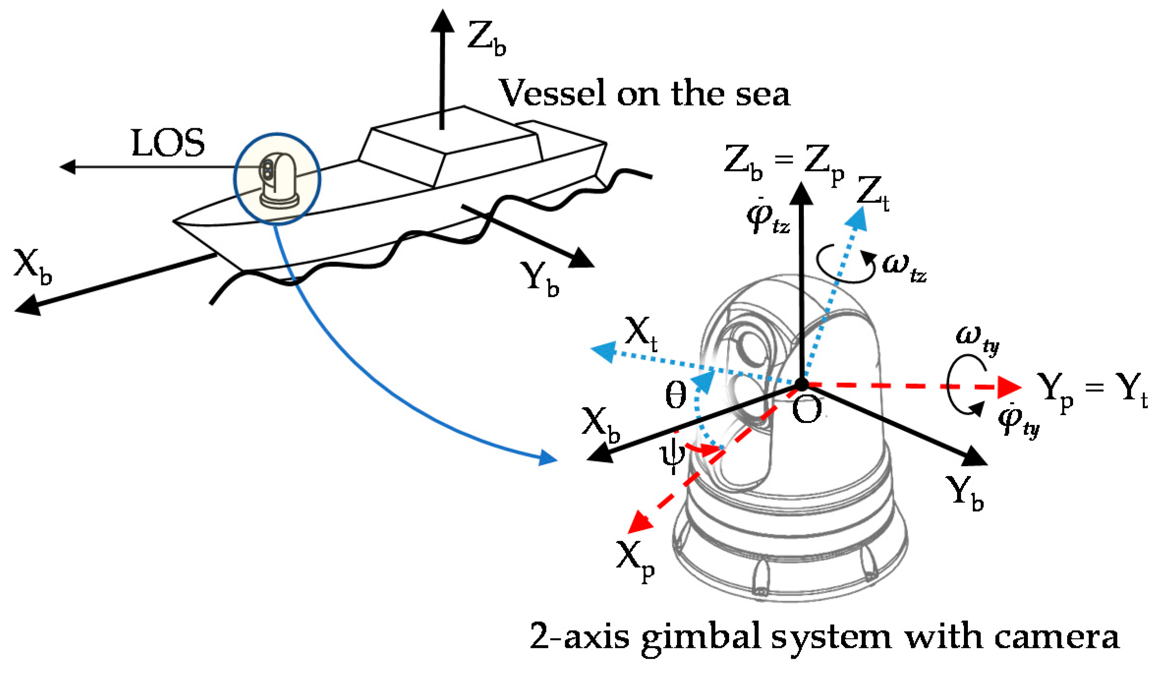
Gimbaled mechanisms are widely used in practical applications where the line-of-sight (LOS) of an optical sensor needs to be stabilized and steered to track a moving target. Carried on mobile vehicles, these mechanisms are electromechanical structures consisting of two or more independent channels. Each of these channels orientates about an axis different from the others. The optical sensors, such as vision and thermal cameras, radars, and laser sensors, are usually mounted on the inner channel of the gimbal. However, in some configurations, the sensors are fixed to the vehicle carrying the gimbal where mirrors or other optical elements are mounted. Moreover, a gyro or a set of gyros is used to measure rotational motions in the inertial space and feedbacks the data to the control systems. Requirements for these systems vary depending on applications. On one hand, in applications such as mapping, security, communications, and handheld cameras, the control problems mainly focus on attenuating unmeasured disturbances affecting the optical sensors. On the other hand, in target tracking, surveillance, missile guidance, gun-turret control, and astronomical telescopes applications, the sensor is required to track the target precisely in real time. The complexity of the system dynamics, unpredicted target direction, and disturbances make these tasks challenging even though control problems of gimbal systems have been studied for decades. In 2018, a special issue of IEEE Control Systems Magazine was dedicated to inertially stabilized platforms and presented several articles overviewing many aspects of this topic [
1,
2].
The gimbal itself is a simple structure, but its dynamics are complex with nonlinear factors, couplings, and disturbances. Mathematical models of the system have been derived from many studies to point out these problems. In [
1], the kinematics of a multi-axis gimbal was devised in terms of the trigonometric functions of the platform and rotations of the gimbal channels. Analyzing these equations highlights the kinematics coupling and unwanted effects on the LOS motion. Meanwhile, the representation of the simplest one-axis gimbal dynamics was introduced in [
2], and the dynamics of the two-axis one had been derived in several studies [
3]. Recent studies, such as [
4,
5,
6,
7,
8], analyzed in detail the system models with complex nonlinearities induced by cross-couplings, parameter uncertainties, and external disturbances. Thus, there is a need to design an effective control system so that robust stability and superior performance are achieved.
In order to attain these objectives, numerous control approaches were suggested. Classical control strategies of a gimbal system proposed two control loops: an inner rate or stabilization loop inside an outer tracking loop. The inner loop compensates for disturbances, and the tracking loop ensures that the sensor LOS remains pointing towards the target [
2]. Additionally, in [
3], two control methods have been deployed: direct stabilization using feedback signals from the LOS orientation and indirect stabilization based on the base motion. However, modern control techniques allow the design of a single controller that can both track the target and suppress disturbances. The popular schemes used to control gimbal mechanisms are the sliding mode control (SMC), robust control, and active disturbance rejection control, thanks to their robustness and effectiveness when facing disturbances. For instance, an integral sliding mode controller combined with an observer, namely a reduced-order cascade extended state observer [
6] and a disturbance/uncertainty estimator [
9] were suggested. A terminal SMC and a high-order sliding mode observer were designed in [
5] to overcome the cross-coupling and external disturbances that influence the system. Moreover, a backstepping sliding mode controller with an adaptive neural networks approach was designed in [
7], and a super-twisting sliding mode controller (STSMC) was introduced in [
10]. On the other hand, robust control theory was applied in [
8,
11] and several other studies. Especially, the study in [
8] introduced a new robust double active control scheme for a two-axis gimbal system, where an inner active compensator was combined with a feedback controller designed based on
framework. This configuration was introduced so that the system was able to suppress both external disturbances and mutual interferences. However, the design process of most of these controllers neglected the nonlinear characteristics of the system. Instead, they were treated as unknown disturbances and estimated by an observer.
Furthermore, practical gimbal systems and their components cannot operate ideally, which can significantly affect the performance of the control systems. Actuator saturation, gyro output parameterization, and communication network may be listed among practical factors contributing to performance deterioration. However, very few studies considered them while designing the controllers. For example, the study in [
7] dealt with a gimbal system with saturated actuators that degraded the system performance. Thus, the authors applied an auxiliary function to define the effect of saturation and obtained a suitable SMC law. However, the framework of this function was not thoroughly explained. Additionally, the authors in [
10] considered quaternion feedback from the gyro sensor in designing a super-twisting controller for a three degrees-of-freedom (DoF) inertial stabilization platform. Generally, gyro-type sensors provide several ways to represent the 3D orientation of an object in space, namely Euler angles, quaternions, axis angles, and rotation matrices. These concepts are different from the concept of angular position, angular velocity, and angular acceleration that are usually used in motion equations. That is the feedback values from the gyros are not the ones expected by the system model.
Besides the abovementioned factors, the time delay is receiving lots of attention thanks to the increasing use of networked control systems and closed-loop actuators. In these systems, a simple controller is integrated with an actuator, and they form a servo-system that works as a node in the network. In master and slave network configurations, the main controller works as the master, while sensors and actuators are slaves. Data, including sensor feedback and control signal data, are transmitted via a shared network or wireless connections. The study of Baillieul and Antsaklis [
12] reviewed the problems of control and communication in networked real-time systems. Communication time, which introduced the delay time to the system inputs and outputs, was listed as a challenge that reduces the system performances. An overview article from Richard [
13] recalled the characteristics of delay systems and summarized available approaches for their control. In this article, it was stated that the delay systems, both state or input delay, retard or neutral system, usually had bad reputations of system stability and performance. However, while most of the developed techniques have been proved to be effective for state delay systems, controlling input delay systems is more complex and difficult to deal with.
Several approaches have been suggested for input delay systems, namely predictor-like control, robust control, and sliding mode control. A classical hypothesis in the modeling of physical processes is to assume that the future behavior of the deterministic system can be summed up in its present state only. The idea of the predictor control is to establish an expression of the delay-free controller by predicting values of the state and the output ahead of time. The prediction can be achieved by either a state predictor technique, reduction transformation [
14], Smith predictor technique [
15], or inverse backstepping transformation [
16,
17,
18]. They have been claimed to be able to achieve a globally asymptotic stability even with time-varying delays; however, the system should be simple and linear. A combination of backstepping and adaptive techniques (in [
19,
20,
21]) was introduced for input-delay systems represented in a strict-feedback form with uncertainties to achieve—in the best cases—semi-uniform ultimate boundedness of systems. In addition, by taking advantage of modern hardware, more complex control techniques can be implemented with delay systems, such as aperiodic sampling [
22] and model predictive controller [
23]. Otherwise, by treating the difference between the current and delayed control signals as input disturbance, the control objective becomes the attenuation of the matching disturbances, which the SMC and robust control schemes are well known to be able to deal with. In [
13], several research studies using these two methods have been listed, and most of the time, even matching additive disturbance cannot be completely rejected. This implies the ultimate boundedness instead of the asymptotic convergence. For example, the study in [
8] used the same kind of actuators and communication network, and neither the proposed robust double active controller nor the integral sliding mode was able to effectively reject the influences of the time delay in the system. In [
24], the sliding mode algorithm was used to design an observer that estimates the matching disturbances, then reconstructs the states and delays for a system with input delay. However, it is worth noting that any estimation from an observer is always lagging behind the true values for some time. Along with the available delay time in the input channel and the limitations of the system bandwidth, a combination of a controller and an observer may lead to deterioration of the system performance and the system stability. Thus, the abovementioned approaches in [
4,
5,
6,
7,
8,
9,
10,
11], where the common control technique is a combination of the main controller and an observer, might not be suitable for input-delay systems.
Therefore, a novel nonlinear controller for a two-axis gimbal system is designed in this paper to cope with the system complexities and constraints, namely nonlinear dynamic characteristics, gyros feedback parameterization, and system delays. Designed based on the backstepping technique and Lyapunov stability theory, the proposed control scheme preserves the system stability, and accurate real-time tracking performances were achieved. The design procedure of the proposed controller is presented in detail. Simulation and experimental studies were conducted to evaluate the proposed control strategy. Comparison studies were conducted between the proposed control system and an STSMC. Accordingly, the contributions of this paper are listed as follows:
A mathematical representation of the two-axis gimbal system is derived, taking into consideration the Euler angle feedbacks and the input delay time.
A novel nonlinear backstepping controller is introduced for the two-axis gimbal systems to overcome the abovementioned difficulties.
Simulation and experimental results validate the effectiveness of the proposed controller.
The remainder of this paper is organized into five sections. The system mathematical model is described in
Section 2.
Section 3 presents the design process of the controller and stability analysis. Simulation and experimental studies are conducted in
Section 4, where the frequency and time responses of the controlled system are analyzed. Finally, conclusions are drawn in
Section 5.
4. Simulation and Experimental Studies
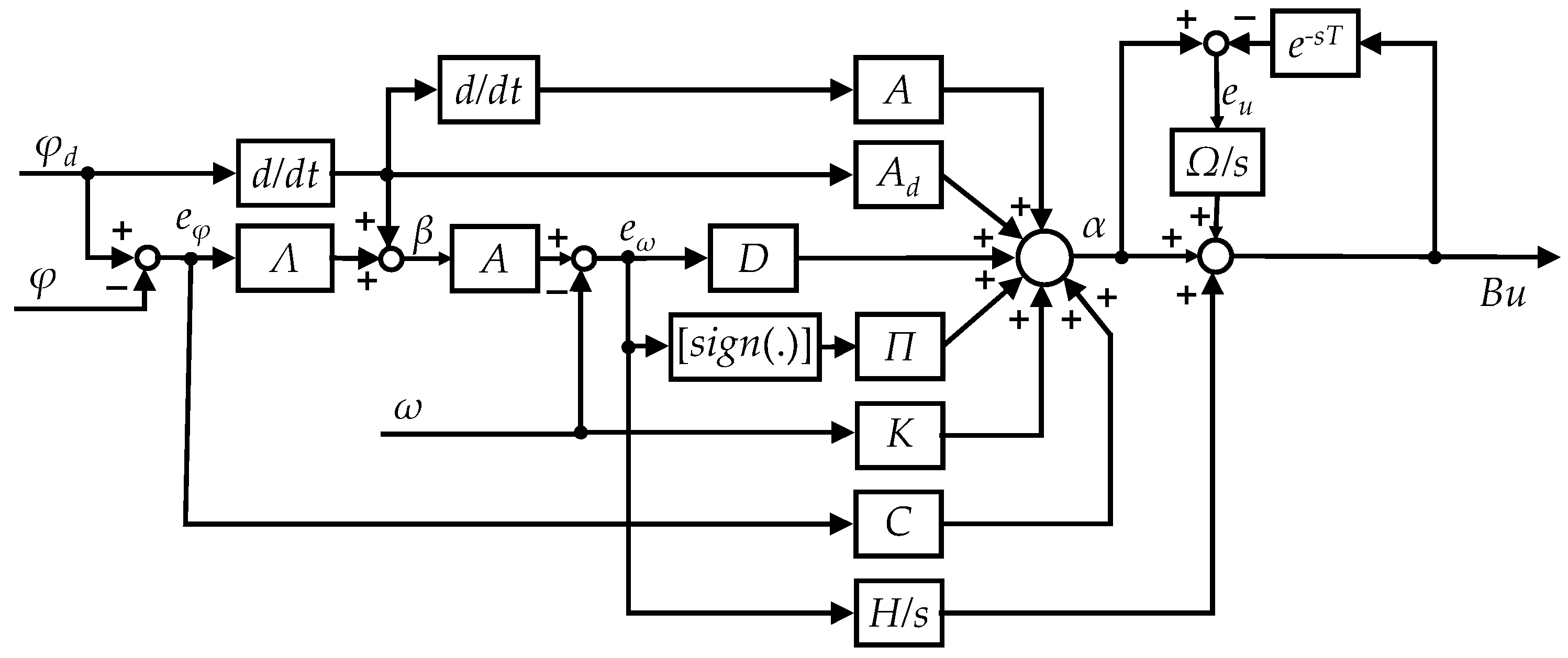
In this section, the proposed controller designed in Equation (29) is investigated. By comparing the performance of the STSMC in Equation (31) and the delay-free BC in Equation (17), the efficiency of the proposed control system is evaluated.
The configuration of the target system, the two-axis gimbal, is illustrated in
Figure 3.
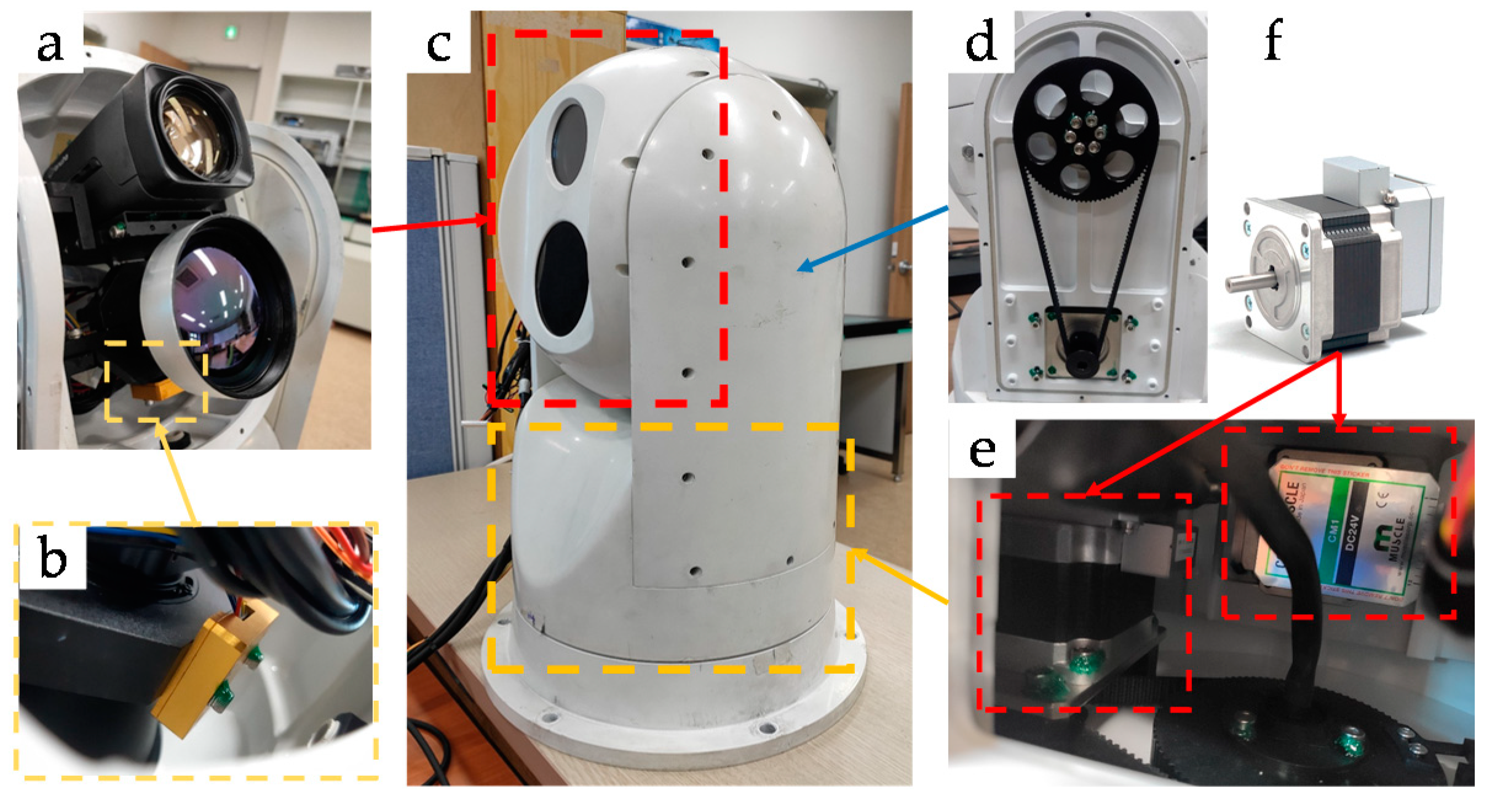
First,
Figure 3c shows the overall view of the system. The system’s payload is a set of cameras, including a vision camera and an infrared thermal imaging camera, as shown in
Figure 3a. Their orientations are sensed by an attitude heading reference system (AHRS) attached underneath,
Figure 3b. Assembled at the side of the gimbal, a belt and pulley mechanism transmits the rotation from the driving shaft of the tilt actuator to the tilt channel with a reduction ratio (
Figure 3e). The actuators are two integrated servo systems COOLMUSCLE CM1-C-23S30—as shown in
Figure 3f—each of them is controlled with a rate command sent through the RS-232 communication network. The sampling time of the control system is 0.02 [s], while the average delay time is three times larger, a value identified based on experimental results. Real-time tracking is an important requirement for gimbal systems in ocean surveillance applications. For instance, when the camera in
Figure 3a is tracking a faraway moving target, the operator is obliged to zoom in on the target for better visualization. In this case, the field of view of the camera is so small that a small tracking error or a moment of lagging can make the target disappear from the monitor; thus, the tracking fails.
Simulation tests in this study were conducted with the system model introduced in Equation (9) and the proposed controller alongside two others. Furthermore, experimental studies were performed on the target system. The system parameters are shown in
Table 1, while the gain matrices of the controllers are presented in
Table 2.
4.1. Simulation
In the simulation scenario, the gimbal has to track a mobile target moving along a circular route with different speeds. This task creates the desired trajectories for the tilt and the pan orientations for the inner gimbal given by:
where
is the maximum value of the angle, and
is the desired frequency value in proportion to the target’s speed. As abovementioned, the delay limits the bandwidth of the system. Therefore, by performing simulations with a chirp-type reference based on Equation (33), the frequency response and the influence of the time delay are evaluated.
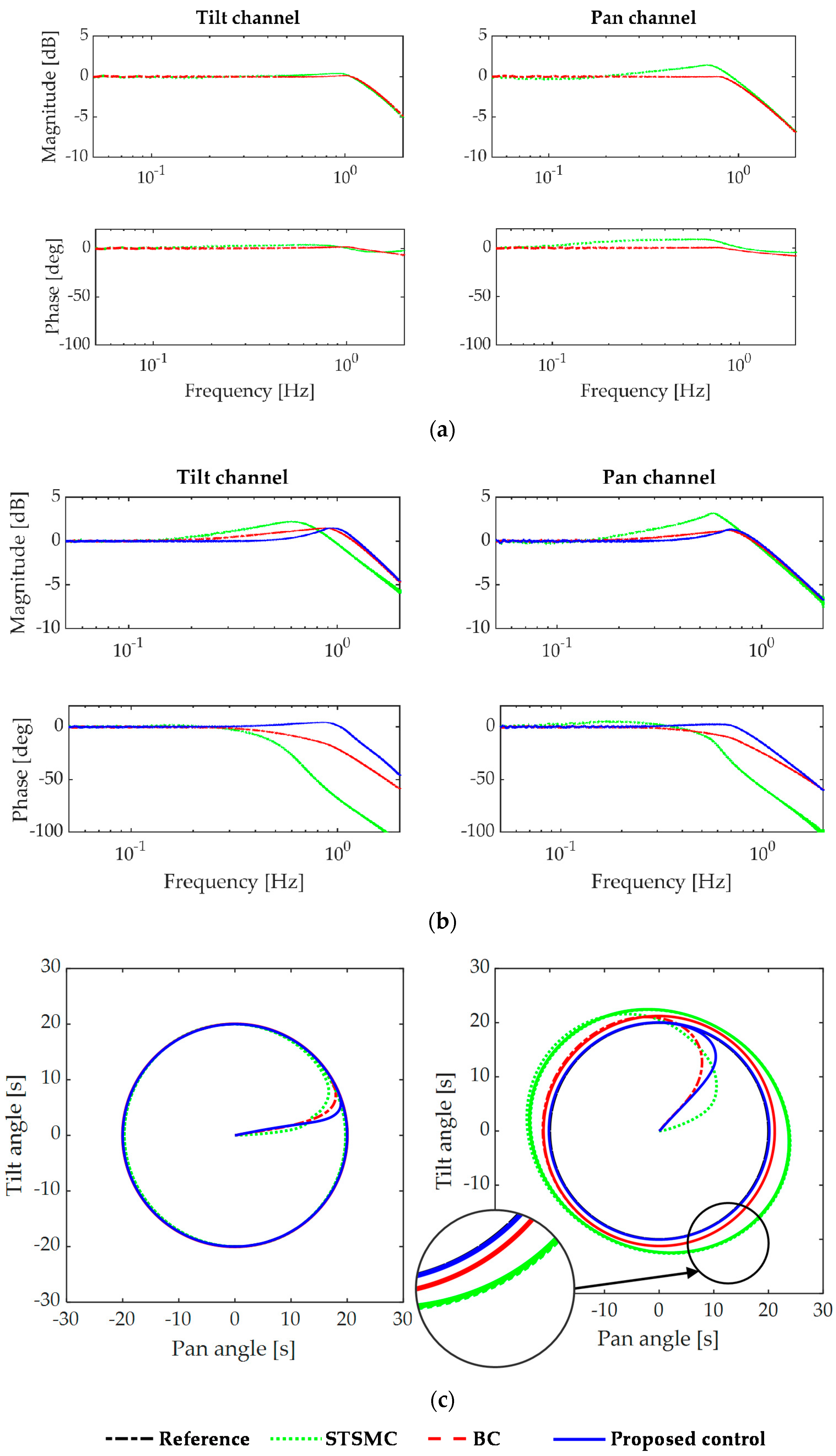
Simulation results are illustrated in
Figure 4 in which
Figure 4a,b show the frequency responses of the two channels with a delay-free input and a 0.06 [s] delay time, respectively. The responses are drawn from the Fourier transforms of the simulation outputs and the reference signals. This is similar to the concept of the complementary sensitivity function of a linear system, where the magnitude response shows the ratio of the amplitude of the output and the reference, and the phase response indicates the phase lag. The frequency responses of the gimbal system with no delay controlled by the STSMC and the BC are illustrated in
Figure 4a. The BC controls the tilt and pan channels accurately in real time with slow-varying reference frequencies up to 1 and 0.8 [Hz], respectively. The values of 0 [dB] in magnitude and 0 [deg] phase shift prove these statements.
On the other hand, using the STSMC, small errors of the amplitude and the phase are seen in the tilt channel response. However, great overshoot and incorrect phase shifts are present in the pan channel response. A possible explanation is the neglect of trigonometric nonlinearities in system dynamics while designing the pan channel controller.
Simulation results of the system with input delay are shown in
Figure 4b, and the influence of the time delay is easily noticed. The STSMC, BC, and the proposed controller ensure the results of 0 [dB] and 0 [deg] when following low-frequency trajectories. Thus, accurate tracking performances are achieved both in terms of magnitude and real-time characteristics. However, when the target moves faster, different control performances are obtained from the control schemes. Both the STSMC and the BC perform much worse than they do with the delay-free system. The frequency responses of the tilt channel in
Figure 4b show that the controllers based on the backstepping approach increase the bandwidth of the system up to 21% compared to the system controlled by the STSMC. These bandwidths are smaller than the ones shown in
Figure 4a, which shows the significant effects of such a small time lag. In their controllable range, the STSMC performs poorly, resulting in the highest magnitude among the three controllers. Starting from 0.2 [Hz] and increasing the frequency, the faster the target becomes, the bigger the amplitude of the system response. Besides, the phase shift begins to decrease at 0.3 [Hz]. Thus, the tracked trajectory using STSMC is far behind the reference. In contrast, the proposed control system provided the most accurate real-time tracking performance on a larger frequency range. The magnitude was maintained at 0 [dB], but starting from 0.4 [Hz], the magnitude began increasing; however, its peak was not higher than that of the BC. The phase lag was also small when the proposed controller was used, as shown in the phase shift plot.
In the case of the pan channel with the input delay, the control bandwidth did not improve much compared to the STSMC. However, both the magnitude and the phase responses improved in the controllable range. Two examples, in particular, illustrate the aforementioned analyses, the frequencies 0.05 and 0.3 Hz, as shown in
Figure 4c. These results validate the proposed controller as the one that preserves accurate tracking performance of the system on the largest frequency range.
4.2. Experimental Studies
Experimental studies were performed in two scenarios. The first one is similar to the simulation tests; the gimbal is tracking a moving target. In the second experiment, the system follows step-type references, similar to the point-to-point tracking. Both reference signals are rich in information that help evaluate the effectiveness of the control system.
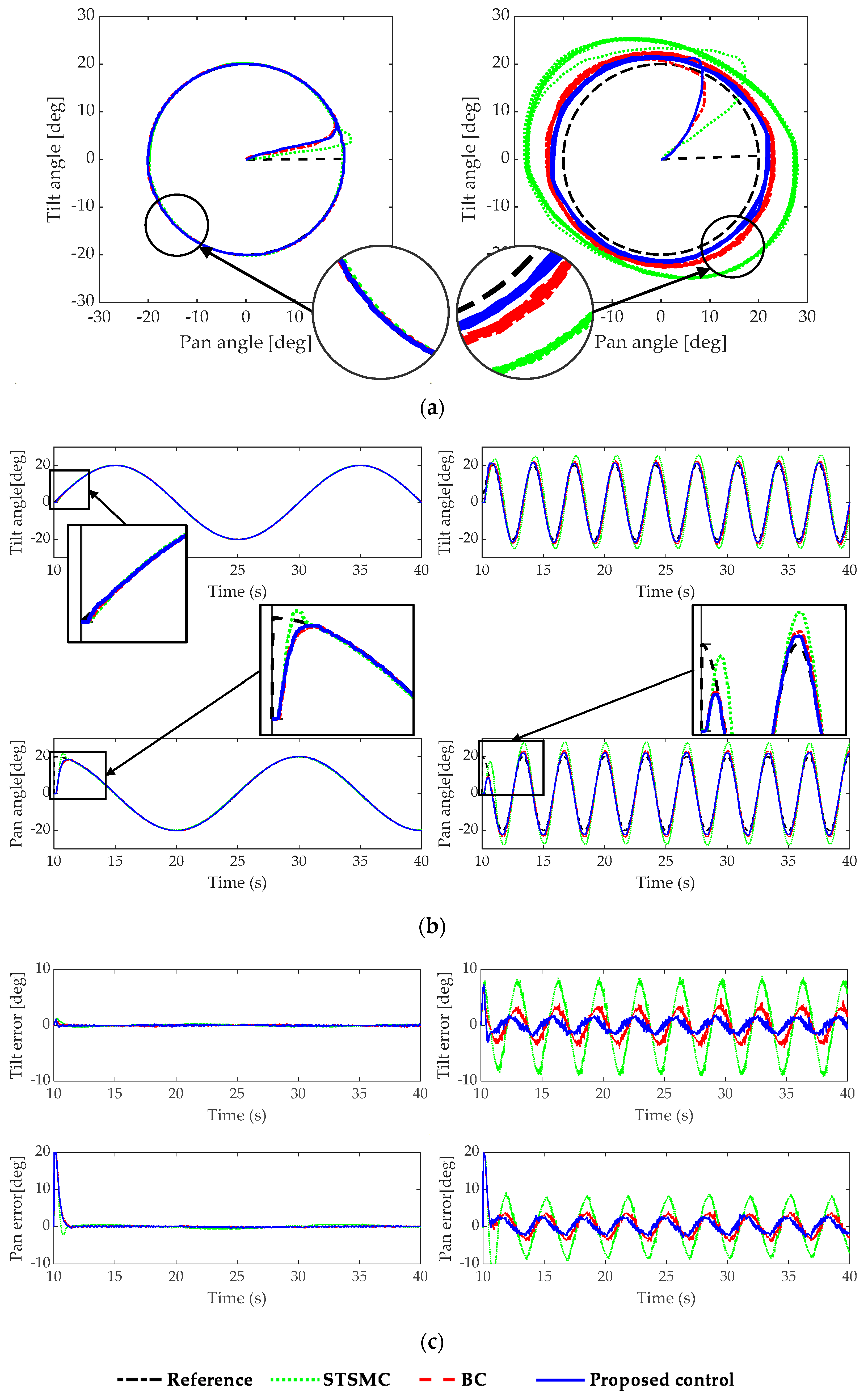
In the first experiment, the reference signals are chosen as in Equation (33) with a 90 [deg] difference in phase and 20 [deg] in radius. The experiments were conducted on a large frequency range to verify the performance of the system controlled by the proposed controller. Two responses at the specific frequencies 0.05 and 0.3 [Hz] are illustrated geometrically in
Figure 5a in a similar fashion to the simulation tests. Details of the time responses of these two frequencies are given in the following
Figure 5b,c. The difference between the responses of the two controllers was small in the case of 0.05 [Hz], but the differences are significant with a frequency of 0.3 [Hz]. The time responses in
Figure 5b,c indicate that the three controllers were able to attenuate the delay after a few seconds and then track the target in real time (the controllers began to operate the system from the 10th second). However, with 0.3 [Hz], the response given by the STSMC showed a greater overshoot and was slightly lagging behind the reference.
These results correspond with the response illustrated in
Figure 4b, where the STSMC gives the highest increase in magnitude and phase lag at 0.3 [Hz]. The proposed controller showed the best performance, as seen in the controlled system response in
Figure 5a,b, and a minimal tracking error as shown in
Figure 5c. In addition, root-mean-square error values in
Table 3 give numerical merits assessing the effectiveness of the proposed controller in comparison with the other control systems.
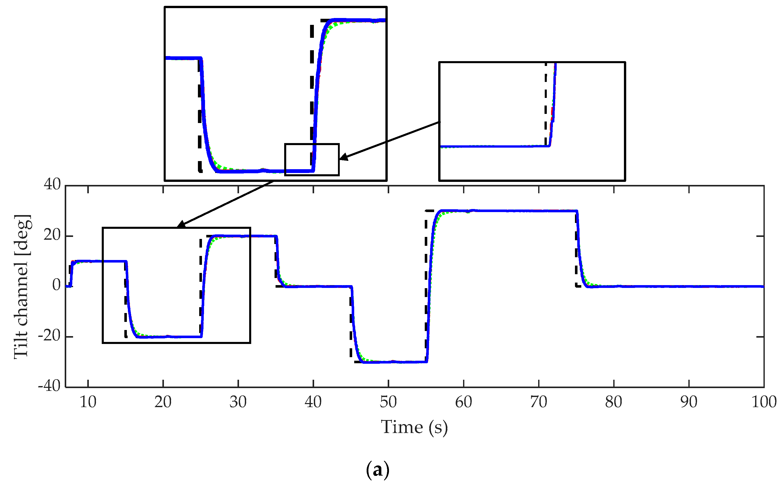
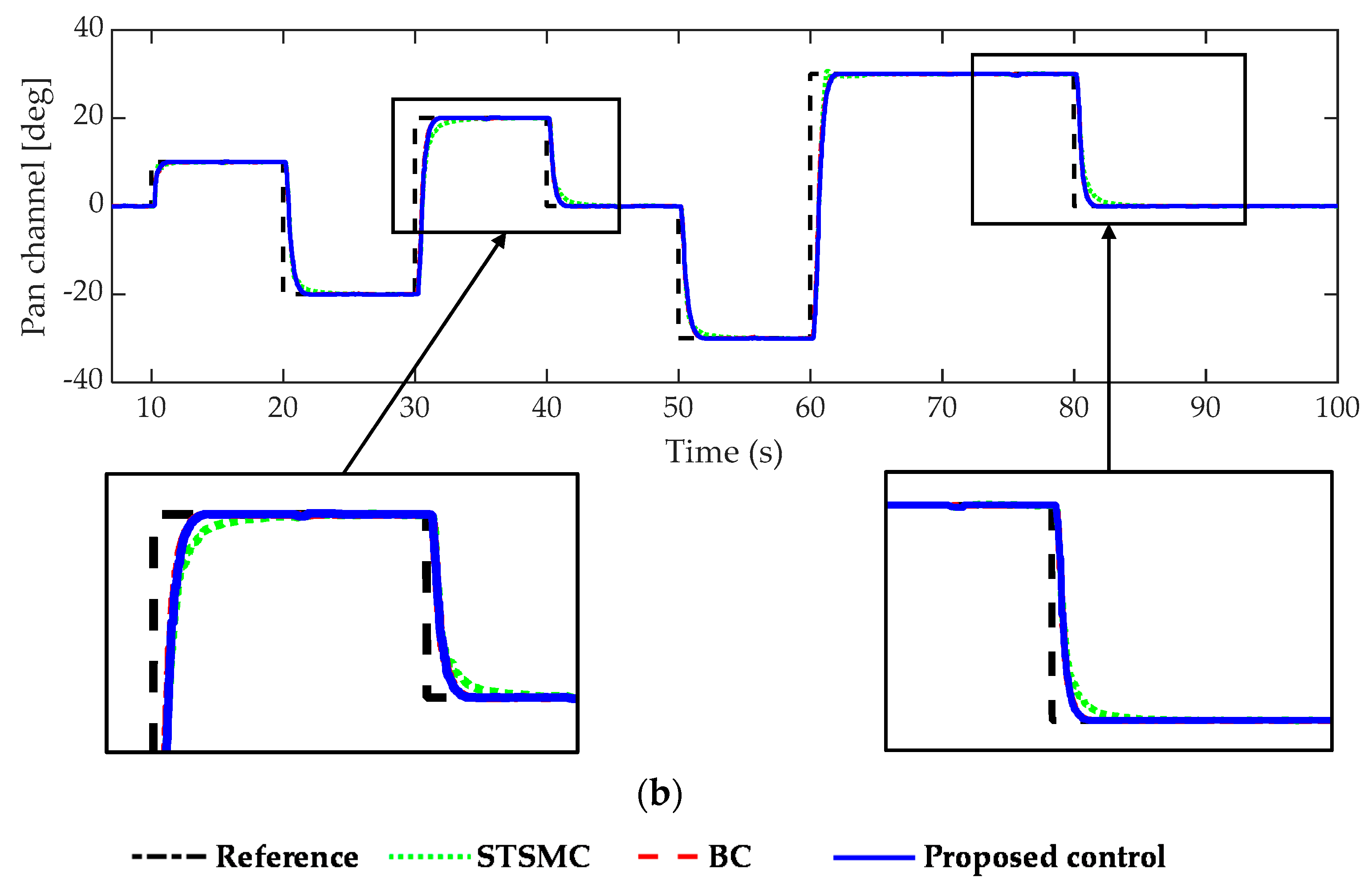
The second experiment was conducted with a step-type reference. The response of each channel is shown individually in
Figure 6a,b. The closeup figure at the top right of
Figure 6a shows clearly the delayed response. On the other hand, all the controllers were able to control the system to orientate towards the desired positions with no overshoot and small steady-state errors. The closeup figures, in particular, show that the proposed controller provides a better transient response so that the desired positions are reached in a short period of time.


