Nonlinear Wave Evolution in Interaction with Currents and Viscoleastic Muds

Abstract

A numerical model is extended to investigate the nonlinear dynamics of surface wave propagation over mud in the presence of currents. A phase-resolving frequency-domain model for wave-current interaction is improved to account for wave modulations due to viscoelastic mud of arbitrary thickness. The model compares well with published laboratory data and performs slightly better than the model with viscous mud-induced wave damping mechanism. Monochromatic and random wave simulations are conducted to examine the combined effect of currents, mud-induced wave dissipation and modulation, and nonlinear wave-wave interactions on surface wave spectra. Results indicate that current effects on wave damping over viscoelastic mud is not as straightforward as that over viscous mud. For example, while opposing currents consistently increase damping of random waves over viscous mud, they can decrease damping over viscoelastic mud due to high variations in frequency-dependent damping stemming from mud’s elasticity. It is shown that a model that assumes the mud layer to be thin for simplification can overestimate wave damping over thick mud layers.

1. Introduction

Interactions among gravity waves, currents, and bottom sediments in the coastal environment are complex. In areas with strong currents such as inlets or river mouths, hydrodynamic forces induced by waves and currents resuspend and transport sediments while bottom sediments can attenuate waves and currents through bottom friction or viscous damping within the sediment layer. To add to the complexity, waves and currents interact and their interactions can affect the kinematics of flow field and its impact on sediment transport. Understanding these interactions enable coastal engineers and scientists to better estimate wave forces, understand the fate of sediments in the coastal zone, and predict shoreline erosion.

Sediments in most coastal areas are heterogenous with varying proportions of clay. A well-known process over bottom mud is attenuation of surface waves which is considerable compared to sandy beds e.g., [1]. Wave-mud interaction has been the subject of many recent studies that explore spectral wave evolution [2,3,4,5,6]. However, only a few studies have considered the effect of currents on wave-mud interaction e.g., [7,8,9,10,11,12]. However, substantial mud deposition occurs in river deltas and strong currents can interact with wave and mud in the vicinity of river inlets. Therefore, a model that incorporates current effects on waves can better predict mud-induced wave attenuation. Interaction between waves and currents change the linear and nonlinear properties of surface waves [13]. Doppler shifting of frequencies is a linear effect of currents on waves that can result in nonlinear energy transfer across the wave spectrum [12]. Other nonlinear effects of currents have been previously studied focusing on large amplitude waves in the presence of adverse currents [7], waves near blocking condition [8,9], and deep water waves [10,11] and wave-wave interactions in shallow water for regular [14] and irregular [12] waves.

A reliable model for wave evolution over mud requires an accurate characterization of mud behavior. Various rheological models have been adopted for this purpose among which the most common ones are viscous fluid e.g., [15,16], viscoelastic medium e.g., [17,18,19,20,21], and Bingham plastic e.g., [22,23,24,25]. Since mud exhibits different behaviors depending on its state of consolidation and composition e.g., [26], a single rheological model may fail to predict mud behavior under a wide range of hydrodynamic forcing. Among the aforementioned rheological models, viscoelastic fluid and solid models can predict wave dissipation over the widest range of wave forcing and sediment characteristics [27]. To study wave damping over viscoelastic mud, Macpherson [17] developed the formulation for a two-layer system composed of clear water overlying a layer of viscoelastic Voigt solid. Piedra-Cueva [28] extended the work to include the effects of boundary layers at the water/mud interface (or lutocline). More recently, Liu and Chan [20] (referred to as LC hereafter) derived a model for surface wave damping rate assuming that the thicknesses of the mud layer is small and is of the same order of magnitude as the bottom boundary layer. An advantage of the LC model is that unlike Macpherson [17], the damping rates are explicit function of parameters in the problem.

An important characteristic of viscoelastic mud is the resonance effect. As a result of resonance, surface wave frequencies in the proximity of natural frequency of oscillation of the mud layer undergo stronger damping than other frequencies in a spectrum. Since surface waves undergo substantial evolution in shallow water due to nonlinear wave-wave interactions, predicting waves in shallow water ideally requires a model that resolves interaction among waves and those between waves and their surrounding environment, namely sediments, vegetation, or structures. Phase-resolving wave models represent these interaction explicitly to varying degrees whereas phase-averaged models parameterize them, resulting in potential inaccuracies. In a recent study, Tahvildari and Sharifineyestani [6] incorporated the LC model in a phase-resolving frequency-domain model and studied mud’s elastic effect on evolution of regular and irregular waves over mud. Model results showed that neglecting mud’s shear modulus can result in substantial errors in predicting bulk wave properties, such as root-mean-square wave height ($H_{rms}$), as well as nonlinear energy transfer across spectrum that affects the shape of the spectrum.

Mud can dissipate surface waves through direct and indirect mechanisms. Direct damping involves damping of surface wave energy due to viscosity in the mud layer which is a first-order phenomenon meaning that it occurs even if only linear motions are considered. However, field and laboratory experiments indicate that high [1,29] and low [30] surface wave frequencies exhibit higher damping than what is anticipated merely from direct dissipation. Numerical simulations and theory show that high-frequency dissipation is due to nonlinear energy transfer from short to long waves which are directly damped by the mud [2,5,29] while low-frequency dissipation is due to nonlinear energy transfer from low to high frequencies due to short wave modulation [21,31]. Another indirect mechanism for surface wave damping can be the generation of interfacial waves over lutocline by surface waves and their dissipation due to mud’s viscosity. The mud/water system can be idealized as a two-layer configuration that supports the generation of interfacial waves. One mechanism of generation of interfacial waves, relevant to coastal systems, is the resonant excitation of a pair of interfacial waves by a single surface wave [32,33,34,35]. Interfacial waves are subject to damping through viscosity within the mud layer as well as dissipation within interfacial boundary layers [35,36]. While the process is a second-order phenomenon and transient, it can result in substantial surface wave energy dissipation if it persists for long time.

Numerical wave models have enabled studying wave-mud interaction in complex wave conditions. Among mud rheological models, the viscous fluid model has been implemented in wave models most commonly. The phase-averaged models SWAN [37,38] and WAVEWATCH III [39] as well as phase-resolving models e.g., [2,5] have used the viscous mud-induced wave damping mechanisms. Kaihatu and Tahvildari [40] extended the Kaihatu et al. [2] study to account for the effect of currents on mud-induced wave dissipation and showed that the damping dominates spectral evolution even in the presence of relatively strong currents. Their results show that, in agreement with earlier studies, counter-propagating currents increase wave damping while co-propagating currents reduce it. It is noteworthy that increase in wave attenuation over counter-propagating currents is independent of bottom type and has been observed over other rough beds e.g., [41]. Recently Tahvildari and Sharifineyestani [6] incorporated a mechanism for surface wave modulation and dissipation by viscoelastic mud in a nonlinear frequency-domain model [2]. Their results show that bulk wave characteristics such as $H_{rms}$ are dictated by direct damping which is highly influenced by resonance of the mud layer. Furthermore, the relative magnitude of the spectral peak frequency and mud’s resonance frequency was found to be a key factor in the shape of the damped spectrum. It was also shown that similar to viscous mud, subharmonic interactions result in damping of high frequencies over viscoelastic mud, but the damping rates vary with mud’s shear modulus. All in all, it was shown that neglecting mud’s elasticity can introduce significant errors in bulk wave characteristics as well as spectral shape.

In this research, we extend the model of Kaihatu and Tahvildari [40] by generalizing the mud rheology to a viscoelastic solid. We utilize two models to represent mud-induced damping and modulation of surface wave in the wave model, namely the LC model and Macpherson [17]. Implementation of the latter model enables applying the wave model to muds of arbitrary thickness by eliminating the limitation of thin-mud-layer assumption imposed by LC. Therefore, the present model provides a more comprehensive predictive tool for wave propagation in coastal waters.

The paper is structured as follows. Following this introduction, Section 2 discusses the wave-current-mud interaction model, Section 3 presents model simulation results for current effects on evolution of monochromatic and random waves, Section 4 discusses the applications and limitations of the model, and Section 5 provides concluding remarks.

2. Numerical Model

The coupled wave-current-mud interaction model integrates the wave-current interaction model of Kaihatu [12] which simulates nonlinear propagation of waves in the presence of currents, and two mechanisms for mud-induced surface wave evolution formulated in LC and Macpherson [17].

2.1. Nonlinear Wave–Current Interaction Model

There have been numerous earlier studies on wave-current interactions which showed that background currents can strongly affect oceanic surface gravity waves e.g., [42]. To carry out a comprehensive investigation of wave-current-mud interaction, vertically varying currents and the effect of resulting shear and vorticity on waves need to be considered as it is well-known that currents affect wave kinematics within and outside the bottom boundary layer e.g., [43,44]. It is noted, however, that an irrotational theory that uses depth-averaged velocity can provide a good approximation for rotational theory [42]. Since the focus of this study is to begin to investigate current effects on nonlinear spectral evolution over viscoelastic mud, the current is assumed to be simply constant with depth. Based on this assumption, the shear and vorticity are neglected and the flow can be assumed irrotational.

The wave-current interaction model used in this study is developed by Kaihatu [12] based on the mild-slope equations [45], which explicitly solves the nonlinear triad interactions. The model is applicable to weakly two-dimensional flows as it uses the parabolic approximation [46]. The linear characteristics of wave-current interaction are adequately represented in the model by enforcing the conservation of wave action, which in one horizontal dimension is given by Bretherton and Garrett [13]:

$$\frac{\partial }{\partial x}\left(\frac{C_{g}E}{\sigma }\right)=0.$$

(1)

$C_g$ is the wave group velocity, given by,

$$C_g=\frac{C}{2}\left(1+\frac{2kh}{sinh2kh}\right),$$

(2)

where $C=\sigma /k$ is the wave celerity, $\sigma$ is the intrinsic frequency which is measured with respect to the coordinate system that is moving at the speed of the background current, and is equal to $2\pi /T$ where T is the wave period, k is the wave number, and h is the water depth. $\sigma$ satisfies the dispersion relation as ${\sigma }^2=gk$tanh$\left(kh\right)$. E is the wave energy per unit area, given by,

$$E=\frac{1}{8}\rho g{H}^2,$$

(3)

where H is the wave height. The absolute frequency, $\omega$, is measured with respect to a fixed reference frame, and has the following relationship with $\sigma$,

$$\omega =\sigma +kU,$$

(4)

where U is the ambient constant current which is vertically constant but can change in the horizontal direction. This is consistent with the governing equations which assume irrotational flow and slow-varying depth. The strength of the current is assumed to be $\mathcal{O}$(1). There is a plethora of wave-current interaction models. Since the purpose of this study is to examine nonlinear evolution of waves over mud in the presence of currents and how viscoelasticity of mud affects the process, we use the frequency domain phase-resolving nonlinear model of Kaihatu [12]. The model treats the nonlinear interactions between wave components explicitly, enabling to focus on nonlinear wave evolution. An advantage of the present model is that it can be used to benchmark more comprehensive wave models, for example Reynolds-Averaged Navier Stokes (RANS) models, for their performance in resolving triad interactions. In Kaihatu [12], second-order effects are added to the wave-current interaction model of Kaihatu and Kirby [47] and energy transfer calculations in high frequencies are improved. Here we only describe the main model equation and refer the reader to Kaihatu and Kirby [47] and Kaihatu [12] for more details. The evolution of surface wave amplitude over slowly varying depth in one horizontal dimension (x) is given by Kaihatu [12] in frequency domain:

$$\begin{array}{ccc}\hfill & & \frac{\partial A_n}{\partial x}+\frac{{\sigma }_n}{2\left(C_{gn}+U\right)}\left[\frac{\partial }{\partial x}\left(\frac{C_{gn}+U}{{\sigma }_n}\right)\right]A_n+D_n{A}_n\hfill \\ \hfill & & =\frac{-i}{8\left(C_{gn}+U\right){\sigma }_n}\left(\sum _{l=1}^{n-1}R{A}_l{A}_{n-1}{e}^{i{\mathsf{\Theta }}_{l,n-1}}+2\sum _{l=1}^{N-n}S{A}_l^{*}{A}_{n+1}{e}^{i{\mathsf{\Theta }}_{n+l,-1}}\right)\hfill \end{array}$$

(5)

where subscript n denotes the nth surface wave harmonic, $A_n$ is the harmonic amplitude, and $C_{gn}$ and $D_n$ are the group velocity and the dissipation rate of the nth harmonic, respectively, and $i=\sqrt{-1}$. The nonlinear interaction coefficients R and S represent the super- and sub-harmonic interactions, respectively, the asterisk denote complex conjugate, ${\mathsf{\Theta }}_{l,n-1}=\int k_l+k_{n-l}-k_{n}dx$, and ${\mathsf{\Theta }}_{n+l,-1}=\int k_{n+l}-k_l-k_{n}dx$. The subscript of the wave numbers in these integrals refer to the wave frequency in the spectrum. The Kaihatu [12] model includes a correction to $A_n$ to account for second-order effects in the dynamic free-surface boundary condition. The resulting corrected harmonic amplitude, $B_n$, is calculated as,

$$\begin{array}{c}\hfill B_n=A_n+\frac{1}{4g}\left[\sum _1^{n-1}I{A}_l{A}_{n-l}{e}^{{\mathsf{\Theta }}_{l,n-l}}+2\sum _1^{N-n}J{A}_l^{*}{A}_{n+l}{e}^{{\mathsf{\Theta }}_{n+l,l}}\right]\end{array}$$

(6)

where I and J are nonlinear interaction coefficients. Equation (5) is modeled with a fourth-order Runge-Kutta scheme [47]. At the leading order, ambient currents modify wave frequencies through Doppler shift. The term $D_n{A}_n$ in Equation (5) represents energy dissipation which can be due any interaction between waves and the surrounding environment, namely depth-limited breaking, mud, or aquatic vegetation.

2.2. Model for Surface Wave Evolution over Viscoelastic Mud

The effects of viscoelastic muds on surface waves include viscous dissipation and frequency modulation. In dissipative media, the wave number or frequency is considered to be a complex wave number and their imaginary part represents a spatial or temporal damping rate, respectively e.g., [17]. Frequency modulation, on the other hand, is represented by changes in the real part of wave number or frequency. Therefore, solving wave evolution over mud requires solving the dispersion relation of a two-layer mud/water system which has coefficients and variables composed of real and imaginary parts. Since the LC model is the thin-mud limit of Macpherson [17], comparison between results using these two models sheds light on the effect of thin-mud-layer assumption on surface wave evolution. Figure 1 represents a definition sketch of the wave-current-mud environment in a two layer system. In this figure, $d_m$, ${\nu }_m$, $G_m$, ${\rho }_m$ are mud’s depth, viscosity, shear modulus of elasticity, and density, respectively and h, ${\nu }_w$, and ${\rho }_w$ represent the water’s depth, viscosity and density, respectively. The surface wave amplitude is denoted by a.

2.2.1. Macpherson Model

Macpherson [17] investigated surface wave attenuation in a two-layer system composed of an inviscid water overlaying a viscoelastic layer of solid that represented sediment and was described by the Voigt model. The governing equation for motion of small amplitude waves in a Voigt solid resembles linearized Navier-Stokes equations if the viscosity coefficient in the Navier-Stokes equation is substituted with a complex term that represents elasticity as well. This effective viscosity coefficient is formulated as,

$${\nu }_{me}={\nu }_m+\frac{i{G}_m}{\sigma {\rho }_m},$$

(7)

where ${\nu }_{me}$ is the effective kinematic viscosity of mud e.g., [17], and the real and imaginary parts represent mud’s viscosity and elasticity, respectively. In this equation, ${\nu }_m$, $G_m$, ${\rho }_m$ are mud’s viscosity, shear modulus of elasticity, and density, respectively. The viscosity of the water is neglected and it is assumed that its density is smaller than that of mud. Also, shear stress and mixing at water-mud interface are neglected. The dispersion relation for this two-layer system wave then derived as [17],

$$\begin{array}{ccc}\hfill & & \frac{{\rho }_w\left({\sigma }^4-g^2{k}^2\right)tanh\left(kh\right)}{gktanh\left(kh\right)-{\sigma }^2}+{\rho }_{m}gk+T^{{}^{\prime }}{k}^3\hfill \\ \hfill & & +{\rho }_m{\left(2k^2{\nu }_{me}-i\sigma \right)}^2\left[\frac{\left(2k^2-\frac{i\sigma }{{\nu }_{me}}\right)\left[l{C}_m{C}_l-k{S}_m{S}_l\right]-2k^{2}l}{\left(2k^2-\frac{i\sigma }{{\nu }_{me}}\right)\left[l{S}_m{C}_l-k{C}_m{S}_l\right]}\right]\hfill \\ \hfill & & -4{\rho }_m{k}^3{{\nu }_{me}}^{2}l\left[\frac{\left(2k^2-\frac{i\sigma }{{\nu }_{me}}\right)-2k\left[k{C}_m{C}_l-l{S}_m{S}_l\right]}{2k\left[l{S}_m{C}_l-k{C}_m{S}_l\right]}\right]=0\hfill \end{array}$$

(8)

where $C_m=cosh\left(k{d}_m\right)$, $C_l=cosh\left(l{d}_m\right)$, $S_m=sinh\left(k{d}_m\right)$, $S_l=sinh\left(l{d}_m\right)$, $l={(k^2-\frac{i\sigma }{{\nu }_{me}})}^{0.5}$ where $d_m$ is the depth of the mud layer, h is the depth of the water layer, and $T^{\prime }$ is the surface tension which is assumed to be negligible here. Solving this dispersion relation for wave number, k, gives the modulated frequency, $k_r$ (Re(k)) and damping rate, $D_m$ (Im(k)). This dispersion relation should be solved numerically, and it should be noted that the roots in the complex plane may be non-unique making the solution procedure at times laborious and the correct root ambiguous [48]. This non-uniqueness problem can make implementation into predictive wave models difficult, unless relevant roots are precalucated and incorporated [49].

2.2.2. Liu and Chan Model

The LC model provides explicit solutions for real and imaginary parts of the surface wave number. The implementation of the solution in spectral wave models is straightforward [6] and the approach eliminates the possibility of obtaining multiple roots. The basic assumption in this formulation is that the mud layer is thin and is of the same order of magnitude as the bottom boundary layer within mud:

$$k_{r}a\approx k_r{d}_m\approx k_r{\delta }_{me}\ll 1$$

(9)

where $k_r$ is the real part of wave number and in non-dimensional form is as follows:

$$k_{r}h=k_{1}h-\frac{{\left(k_{1}h\right)}^2\gamma \left(\frac{{\delta }_{me}}{h}\right)}{sinh2k_{1}h+2k_{1}h}\left[2\lambda -\frac{{\mathsf{\Omega }}_{M}sinh2\lambda {\mathsf{\Omega }}_M+{\mathsf{\Omega }}_{P}sin\left(2\lambda {\mathsf{\Omega }}_P\right)}{cosh\left(2\lambda {\mathsf{\Omega }}_M\right)+cos\left(2\lambda {\mathsf{\Omega }}_P\right)}\right],$$

(10)

where $k_1$ is the surface wavenumber for a single layer fluid in the absence of mud and ${\delta }_{me}$ is the mud boundary layer and given by,

$${\delta }_{me}=\sqrt{\frac{2|{\nu }_{me}|}{\sigma }}.$$

(11)

The spatial damping rate in the LC model, $D_m$, in non-dimensional form is given by,

$$D_{m}h=\frac{{\left(k_{1}h\right)}^2\gamma \left(\frac{{\delta }_{me}}{h}\right)}{sinh2k_{1}h+2k_{1}h}\left[\frac{{\mathsf{\Omega }}_{P}sinh2\lambda {\mathsf{\Omega }}_M-{\mathsf{\Omega }}_{M}sin\left(2\lambda {\mathsf{\Omega }}_P\right)}{cosh\left(2\lambda {\mathsf{\Omega }}_M\right)+cos\left(2\lambda {\mathsf{\Omega }}_P\right)}\right]$$

(12)

where

$$\begin{array}{ccc}\hfill {\sigma }^2& =& g{k}_{1}tanh{k}_{1}h,\hfill \end{array}$$

(13)

$$\begin{array}{ccc}\hfill \lambda & =& \frac{d_m}{{\delta }_{me}},\hfill \end{array}$$

(14)

$$\begin{array}{ccc}\hfill {\mathsf{\Omega }}_P& =& cos\frac{\theta }{2}+sin\frac{\theta }{2},\hfill \end{array}$$

(15)

$$\begin{array}{ccc}\hfill {\mathsf{\Omega }}_M& =& cos\frac{\theta }{2}-sin\frac{\theta }{2},\hfill \end{array}$$

(16)

$$\begin{array}{ccc}\hfill tan\theta & =& \frac{G_m}{\sigma {\rho }_m{\nu }_m},\hfill \end{array}$$

(17)

$$\begin{array}{ccc}\hfill \gamma & =& \frac{{\rho }_w}{{\rho }_m}\hfill \end{array}$$

(18)

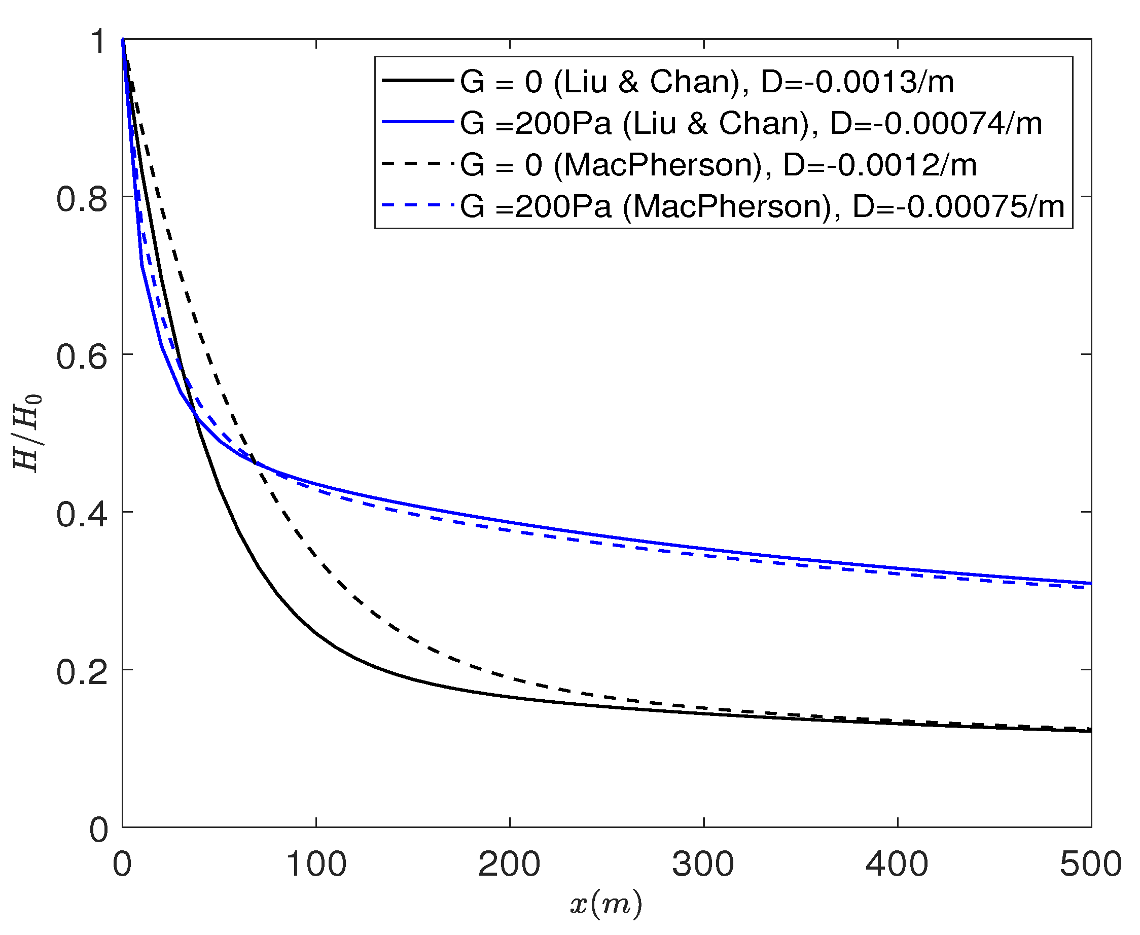
2.2.3. Comparison between Viscoelastic Mud Models

Figure 2 shows variation of damping rates for viscous ($G=0$) and viscoelastic mud with shear modulus of $G=100$ Pa using formulations of LC (Equation (12)) and Macpherson [17] (Equation (8)), and values extracted from the Piedra-Cueva [28] study. In this figure, we used the same parameters that Piedra-Cueva [28] used in their study: $\zeta =\sqrt{{\nu }_m/{\nu }_w}$ = 100, $d_m=0.06$ m, $h=0.30$ m, ${\rho }_m=1370$ kg/m${}^3$, ${\rho }_w$ = 1000 kg/m${}^3$ and wave frequency changes between 0–1.7 Hz. As seen, the variation of damping with $d_m.\sqrt{\omega /{\nu }_m}$ is non-monotinic for both viscous and viscoelastic scenarios and resonance effect, which is manifested by intensified damping, is evident for the viscoelastic case at $d_m.\sqrt{\omega /{\nu }_m}$ of around 2. The highest damping over viscoelastic mud occurs at a frequency equal to mud’s natural frequency of oscillation as it triggers large motions and subsequent viscous damping within the mud layer. All the three formulations show the resonance effect and agree well in the range of parameters used.

Figure 3 shows the variation of $D_m$ with surface wave frequency (f) for various values of mud shear modulus and currents. The damping rates shown in this figure assume that relative viscosity is $\zeta =\sqrt{{\nu }_m/{\nu }_w}$ = 100, $d_m=0.12$ m, $h=1.00$ m, ${\rho }_m=1111$ kg/m${}^3$, and ${\rho }_w=1000$ kg/m${}^3$. The damping rates are smallest at the low and high ends of the frequency range and their variation depends on mud shear modulus and current velocity. Viscous mud consistently causes the highest dissipation rate at low frequencies, regardless of the current magnitude. As seen in the figure, the variation of $D_m$ with f is stronger over viscoelastic muds compared to viscous mud, and the maximum damping rate consistently increases with mud shear modulus up to $G_m=100$ Pa and decreases thereafter. Three current magnitudes of $U=0,\pm 0.15$ m/s corresponding to Froude numbers $Fr=U/\sqrt{gh}=0,\pm 0.05$ are used. As seen, for the viscous case and when $f<0.5$ Hz, the wave damping rate over opposing current is larger than both the cases without current and with co-propagating current. This trend is reversed for $f>0.5$ Hz. The case with viscous mud damping is the same as that studied in Kaihatu and Tahvildari [40] but with thinner mud layer. The same trend in $D_m-f$ variation is seen for viscoelastic muds (Figure 3), and it is noted that reversal in trend occurs at $0.5$ Hz regardless of the value of mud shear modulus. As mud shear modulus increases, current effects on damping rates become more pronounced for frequencies larger than $0.5$ Hz.

The total energy of a frequency over mud depends on direct damping, which is calculated using Equations (8) and (12), and its energy loss or gain due to nonlinear energy transfer across the spectrum [2,5,6]. Therefore, the evolution of surface waves over mud is adequately understood only if a spectral model with capability of resolving nonlinear wave interactions is utilized. To achieve this, we incorporate mechanisms for viscoelastic mud-induced evolution in a nonlinear frequency-domain spectral model for wave-current interaction developed by Kaihatu [12], and apply the coupled model to solve the spatial evolution of surface waves.

3. Model Results

In this section, we first show the validity of the model by comparing with laboratory data. We then utilize the model to demonstrate the effect of wave-current-mud interaction on evolution of monochromatic waves, in the form of cnoidal waves, and random wave spectra.

3.1. Model Validation

As discussed earlier, mud can show different rheological properties under various wave conditions. Properties of the mud layer such as density, viscosity, and thickness can vary widely in the field depending on hydrodynamic conditions, and sediment consolidation and composition. These variations translate to a complex relationship between wave evolution and sediment properties, making it hard to compare observations with predictions from numerical models which highly idealize sediment properties. In contrast, the uncertainty in mud properties and complexities in flow conditions are smaller in laboratory experiments. Therefore, there is a closer correspondence between laboratory experiments and numerical wave models as the models generally assume that mud rheology and other properties are constant over time and space. While there are some laboratory datasets on wave dissipation over mud e.g., [50,51,52], there are a limited number of studies on wave-mud interaction in the presence of currents. Here we utilize two sets of such experimental data, namely Zhao et al. [19] and An and Shibayama [53], to validate our model. The damping rate is calculated using the following equation and is compared with reported values in the two studies:

$$H\left(x\right)=H_0{e}^{-D_s.x},$$

(19)

where $D_s$ indicates surface wave damping rate. For comparison with experiments, we use the wave model with the LC mechanism.

The range of parameters used in Zhao et al. [19] experiments is: $d_m$ = 6–12 cm, h = 24–28 cm, ${\rho }_m$ = 1190–1400 kg/m${}^3$, G = 0.4–25 Pa, wave period = 0.82–1.61 s, and wave height 1.8–10 cm. The range of current velocities in the experiments that were used for validation was -0.18-0.6 m/s. Figure 4 shows the comparison between the damping rates acquired from the wave-current-mud interaction model, in viscous and viscoelastic modes, and the laboratory experiments of Zhao et al. [19]. While the model compares well with the lab data using either viscous and viscoelastic mud mechanisms, it shows a slightly better performance when the viscoelastic mechanism is used. The RMSE of the viscoelastic and viscous mud models are 0.00255 m${}^{-1}$ (with $R^2=0.99$) and 0.00342 m${}^{-1}$ (with $R^2=0.98$), respectively. Figure 5 shows a comparison between the attenuated height of monochromatic waves as reported from several experiments of Zhao et al. [19] and those obtained from the present model. The averaged RMSE for these six cases is $0.0015$ m${}^{-1}$ (with averaged $R^2=0.91$).

The model is compared with the results reported in An and Shibayama [53] for further validation. Mud layer existed only in five of their experiments and those experiments where selected for the validation. The range of parameters in An and Shibayama [53] is: $d_m=8$ cm, $h=26.3$ cm, wave period $=1.01$ s, wave height $=4.48$ cm, and currents $=-19.11$ cm/s to $+18.64$ cm/s. The model with viscoelastic mud compares very well with the experiments (Figure 6) showing a RMSE of 0.0056 m${}^{-1}$ (with $R^2=0.89$).

The values used for mud characteristics that are observed in real field condition are highly variable spatially and temporally, and differ from those used in the experiments used for model validation. In field experiments in the Atchafalaya Bay in the Gulf of Mexico, Elgar and Raubenheimer [30] observed a thick yogurt-like layer of mud with 30 cm thickness lying under a 5-m layer of water. Rogers and Holland [54] reported mud layer with an average thickness of 0.4 m offshore the Cassino Beach, Brazil in water depths ranging from 9–15 m. Liao et al. [4] reported mud depths in the range of 0.03–0.12 m in water depth of 3.20-3.60 m, kinematic viscosity of 0.079–3.17$\times {10}^{-3}$ m${}^2/\mathrm{s}$, and mud density ${\rho }_m$ = 1095–1206 kg/m${}^3$ in the same general area as the experiments of Elgar and Raubenheimer [30] were conducted. Here, similar to Kaihatu and Tahvildari [40], we focus on a combination of water depth and incident wave condition that enable illuminating some aspects of nonlinear evolution over viscoelastic mud in the presence of currents. The mud properties and wave characteristics that are used in the following sections are generally within the range observed in Cassino Beach [54] while the water depth is chosen to be smaller. The setup is comparable to many muddy areas which have long shallow shelves and small variations in bottom bathymetry over long distances. As an example, the shelf near the Marsh Island, Louisiana, USA, is shallower than 2 m over a stretch that is more than 7 km long [40].

3.2. Effect of Currents on Propagation of Monochromatic Waves over Mud

We simulate the evolution of monochromatic waves using cnoidal waves. Investigating the evolution of permanent wave solution is informative since we can assess the combined effect of nonlinearity and frequency-dependent dissipation without the complexities that an irregular wave spectrum entails as it contains numerous frequencies. While multiple frequencies are present in cnoidal waves, they propagate at the same speed and their superposition creates the permanent form solution to Equations (5) and (6) [55]. The permanent form solution used in our simulations is developed by Kaihatu [12] (Equation (5)) and is produced by superposition of the component amplitudes that are harmonics of a fundamental frequency.

Figure 7 shows the variation of amplitude spectrum of cnoidal waves with frequency for different magnitudes of shear modulus, G = 0–200 Pa. The simulations are performed in a domain of length 1000 m in which the mud patch is placed at x = 300–800 m and the grid resolution is $\mathsf{\Delta }x=0.025$ m. A total of 10 harmonics are utilized for generation of a cnoidal wave with the fundamental frequency of $f=0.10$ Hz. The wave height is $H=0.1$ m and the current has three values of $0,\pm 0.15$ m/s corresponding to Froude numbers $F_r=U/\sqrt{gh}=0,\pm 0.05$. The values of mud layer thickness and water depth are 0.12 and 1.00 m, respectively, and the relative viscosity is $\zeta =\sqrt{{\nu }_m/{\nu }_w}=100$. The range of frequency is $0.10\le f\le 1$ Hz corresponding to $0.20\le kh\le 4$. This range of frequencies, mud properties, and water depth were selected such that mud layer remains dynamically thin, consistent with the LC model. Figure 7 shows the initial spectrum at $x=0$ and the spectrum in the lee of the mud patch at $x=800$ m. Generally, it is seen that damping decreases as G increases regardless of the direction of the current. For viscous mud, frequencies smaller than $f=0.6$ Hz experience stronger damping in the presence of an opposing current than a following current. However, this trend changes in larger frequencies such that opposing current results in weaker dissipation. As mud’s shear modulus increases, the frequency at which the change in dissipation trend occurs increases to $f=0.82$ Hz for $G=50$ Pa and $f=0.92$ Hz for $G=100$ Pa. No change in trend is observed for a mud with $G=200$ Pa.

The trend in dependency of mud-induced dissipation on mud’s shear modulus cannot be explained entirely by frequency-dependent damping rates (Figure 3). As discussed earlier, the damping rates in the presence of an opposing current is stronger than those in the presence of a following current for frequencies less than ∼0.5 Hz regardless of shear modulus. However, the point of reversal in this trend is ∼0.60 Hz which shifts to higher frequencies as G increases. Since the LC mode uses linearized equations of motion, it can be concluded that nonlinear wave-wave interactions are responsible for this slight shift. To better understand the reason of this difference, the model is run with subharmonic nonlinear interactions deactivated by setting $S=0$ in Equation (5). Figure 8 shows simulations for cases with and without currents while subharmonic interactions are deactivated. Figure 8 indicates that the variation of amplitudes with frequency follows the pattern of direct damping rate. As seen, when there is no current the amplitude spectrum over viscous mud intersects with viscoleatsic mud with shear modulus of $G=100$, and 200 Pa at 0.5 Hz and 0.65 Hz respectively, which are close to the intersection frequencies of viscoelastic and viscous damping rates in Figure 3. The intensity of damping across frequencies can shift to lower or higher end of the spectrum depending on the direction of the current. As seen in the Figure 8, for a viscoelastic mud with $G=100$ Pa, damping in the presence of a following current is stronger than that in the presence of an opposing current in the range of mid to high frequencies as a following (opposing) current shifts more energy to higher (lower) frequencies where they experience higher (weaker) damping (Figure 3). It is also noted that on the high-frequency end of the spectrum, the change in frequency amplitudes with respect to incident wave spectrum is small. This is in agreement with findings of Tahvildari and Sharifineyestani [6] for waves over viscoelastic mud in the absence of currents and with Kaihatu and Tahvildari [40] for waves over viscous mud in the presence of currents indicating that damping of higher frequencies are due to subharmonic interactions regardless of the magnitude of mud shear modulus, and presence and direction of currents.

Figure 9 shows the spatial variation of the total wave height of the cnoidal wave spectrum, shown in Figure 7, for different values of mud shear modulus. As expected, $H_{rms}$ follows the pattern reported in Kaihatu and Tahvildari [40] for viscous mud where damping in the presence of the following current is less than that in the presence of opposing current. For scenarios with $G=50,100$ Pa, $H_{rms}$ shows undulations with x and at the end of the mud patch the wave is most heavily (weakly) damped in the presence of a following (opposing) current. The trend in $H_{rms}$ variation for viscoelastic mud with $G=200$ Pa is similar to that over viscous mud. The variation of $H_{rms}$ with space is attributed to frequency-dependent damping rate (Figure 3). Most of the energy in the cnoidal wave spectrum is confined in frequencies lower than $0.50$ Hz where $D_m$ is consistently higher for opposing currents for viscous mud and viscoelastic mud with $G=200$ Pa. However, as discussed earlier, $D_m$ is larger for opposing currents for muds with $G=50$ and 100 Pa over low frequencies while $D_m$ for a following currents exceeds that of an opposing current for larger frequencies in the $0<f<0.50$ Hz range.

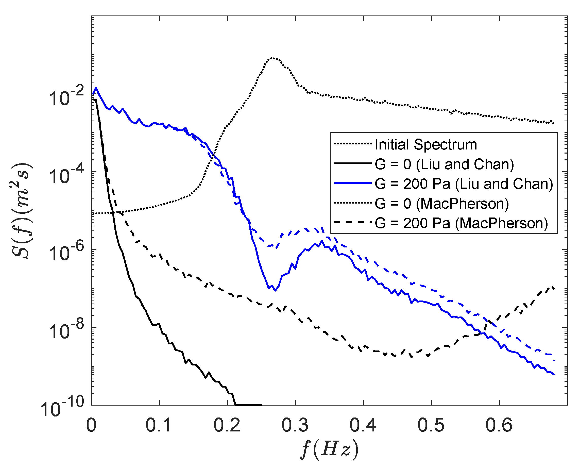
3.3. Effects of Currents on Propagation of Random Wave Spectra over Mud

The random wave simulations use the TMA form spectrum [56] and are performed in a 4900-m long domain (or 70 wave lengths) to ensure that the spectrum reaches a flat equilibrium [12]. The mud patch is placed between 1000–1500 m so that waves undergoes several recurrence cycles [40]. It was noted that the length of the location of the mud patch had negligible effect on results, but selecting the same domain length as Kaihatu and Tahvildari [40] enabled comparing our results with the earlier work. The $H_{rms}$ of initial spectrum and depth of water are $0.24$ m and $2.00$ m, respectively resulting in the Ursell number of $2.08$, where

$$\begin{array}{c}\hfill U_r=\frac{\delta }{{\mu }^2},\end{array}$$

(20)

where $\delta =\frac{H_{rms}}{2h}$, and $\mu =kh$.

The exchange of energy across a spectrum is highly dependent on the Ursell number. Prior work using the same wave model has shown that a spectrum with $U_r=2.08$ exhibits immediate broadening due to strong cross-spectrum energy transfer and does not experience recurrence effect. In contrast, a spectrum with lower $U_r$ of 0.78 preserved its harmonic structure over a longer distance and exhibited recurrent cycling [12]. Here we investigate the evolution of two spectra with peak frequencies $f_p=0.0625$ and $0.26$ Hz. The water and mud properties are selected such that relatively high damping rates are produced: the depth of water and mud layers are h = 2 m, and $d=0.20$ m, respectively, and $\zeta =100$. As an example, this combination results in the resonance frequency of $f_r=0.26$ Hz for $G=50$ Pa. We ran the model for various magnitudes of shear modulus. With these specifications, we chose the frequencies in a range which resulted in $k_r.d_m<1$ corresponding to a relatively thin mud layer. Figure 10 shows the variation of damping rate over f = 0–1.0 Hz. Within this range, f = 0–0.46 Hz, corresponds to thin mud condition with the abovementioned parameters.

Figure 11 shows the evolution of random wave spectra with peak frequency $f_p=0.0625$ Hz over viscous and viscoelastic muds. The initial spectrum and the spectrum at the end of the mud patch (x = 1500 m) are shown for $Fr=\pm 0.15$ and shear moduli of $G=0,100$, and 200 Pa. In the scenario with viscous mud (Figure 11a), higher frequencies clearly undergo stronger damping in the presence of an opposing current though energy level in low to mid-range frequencies in the presence of the opposing current is comparable to that in the presence of the following current at the end of the mud patch. The difference between wave damping in the presence of following and opposing currents is smaller over viscoelastic mud compared to viscous mud (Figure 11b,c). It is noted that spectrum expands quickly in frequency regardless of mud shear modulus and current direction and there is no apparent peaks in the spectrum at the lee of mud. Kaihatu and Tahvildari [40] simulation also indicate that the spectrum with relatively high $U_r$ ($2.08$) undergoes rapid broadening.

Figure 11d–i shows the spatial evolution of several frequencies, namely the subharmonic ($f_p/2$), first ($f_p$), second ($2f_p$), and third ($3f_p$) harmonics of peak frequency. The spectra undergoes some initial evolution where the subharmonic gains energy at the expense of the first three harmonics, but all the frequencies reach a quasi-equilibrium state in 20 wavelengths. It is also noted that dissipation of the subharmonic and all the higher harmonics are stronger over viscous mud than viscoelastic mud. The damping becomes stronger in higher harmonics.

Figure 12 shows the spatial variation of $H_{rms}$. Similar to the case with cnoidal waves, the damping due to opposing current is stronger than that in the following current over viscous mud while the trend reverses as mud shear modulus increases. It is noteworthy that this reversal in trend is consistent with x for all G values for a random wave spectrum and the undulations seen for a cnoidal wave (Figure 9) are not present.

As discussed earlier, a significant property of viscoelastic mud is its capacity to resonate with the surface wave. To better evaluate resonance effects on a random wave spectrum, we simulated the propagation of a spectrum with peak frequency at $f=0.28$ Hz which is equal to the frequency at which maximum direct damping occurs over a mud layer with $G=50$ Pa. Figure 13 shows the spatial variation of $H_{rms}$ for various values of shear modulus of elasticity (G = 0–200 Pa) and currents with $F_r=0,\pm 0.15$. As seen, spatial variability in damping rate of $H_{rms}$ is affected by G and U such that for $G=0$ and 50 Pa, damping rate of $H_{rms}$ is stronger at the beginning of the mud patch compared to the rate at the end of the patch where the $H_{rms}$ reaches an equilibrium. This variability is weaker for muds with $G=0,$ and 200 Pa. On the other hand, the opposing current results in higher damping consistently along the domain for $G=$ 50 and 100 Pa. However, the damping over viscous mud is increased by the opposite current in the beginning of the mud patch and decreased towards the middle and end of the patch. The reverse of this trend applies to the case with $G=200$ Pa where the opposing current intensifies damping up to $x=1250$ m and decreases it onward. The strongest overall damping occurs when the random wave is propagating over a mud with shear modulus $G=50$ Pa as expected from the pattern of direct mud-induced wave damping (Figure 10).

3.4. Propagation of Cnoidal and Random Wave Spectra over Mud of Arbitrary Depth

In this section, the model is used to investigate the effect of mud layer thickness on wave dissipation and evolution. As discussed earlier in Section 2.2.2, LC’s damping mechanism is applicable when mud thickness is at the same order of magnitude as the thickness of the bottom boundary layer. However, the Macpherson [17] model does not apply such a limitation on mud layer thickness. To assess the effect of mud layer thickness on waves, we use the dissipation mechanicsm of Macpherson [17] as the damping coefficient in the model (Equation (5)) and compare the results with the model that uses LC’s model. As before, we use both monochromatic and random wave scenarios.

While the damping rates obtained from the LC and Macpherson [17] models are similar for a thin mud layer (Figure 2), they differ relatively thick muds. As shown in Figure 14, damping rates from the LC model are larger than those obtained from the Macpherson [17] model for viscous mud. For a viscoelastic mud with shear modulus of $G=200$ Pa, the damping rate from Macpherson [17] is slightly larger (smaller) than that calculated from the LC model for frequencies smaller (larger) than $0.22$ Hz and this difference is most substantial around the resonance frequency, which is $0.26$ Hz in this case.

Figure 15 shows the variation of a cnoidal wave spectrum with frequency for $G=0$ and 200 Pa. Mud specifications are the same as those used to calculate $D_m$ in Figure 3 while water depth and mud thickness are $0.8$ m and $0.4$ m, respectively. Also, a wider range of frequency (0–1.85 Hz) is considered. The figure shows the initial spectrum at x = 0 and the spectrum in the end of the mud patch at x = 800 m. Over viscous mud, the LC model clearly overestimates damping in low frequencies while it slightly underestimates it in high tail of the spectrum. Over a viscoelastic mud with $G=200$ Pa, the LC and Macpherson [17] models give comparable damping rates over high and low frequencies but differ considerably over $0.5<f<1$ Hz.

Figure 16 shows the corresponding spatial variation of cnoidal wave height over viscous and viscoelastic muds. The figure shows that for the viscoelastic case with $G=200$ Pa, the Macpherson [17] and LC models are almost identical while for the viscous case, the Macpherson [17] model shows weaker damping than the LC model. The damping rate from both models converge for long mud patches.

Next, we investigate the evolution of random waves over relatively thick mud. The shear moduli used are $G=0,200$ Pa and other mud properties are the same as those specified earlier. Figure 15 shows that in the scenario with viscous mud, the wave model with the LC damping mechanism overestimates attenuation across the spectrum compared to the model with the Macpherson [17] mechanism, consistent with damping pattern of permanent form waves shown in Figure 14. The pattern is more complex for a viscoelastic mud with G = 200 Pa such that for low ($f<0.22$ Hz) and high ($f>0.22$ Hz) frequencies, the Macpherson [17] model gives slightly weaker and slightly higher damping compared to the LC model, respectively. As seen, the distinction between two models is stronger for the case with viscous mud compared to viscoelastic mud. The same result is seen in Figure 17 which shows the spatial variation of random wave $H_{rms}$. As seen, similar to cnoidal wave scenario for the viscoelastic case with $G=200$ Pa, the Macpherson [17] and LC models are almost identical while for the viscous case, the LC model shows stronger damping than the Macpherson [17] model. Comparing Figure 16 and Figure 17, one can conclude that cnoidal waves undergoes stronger attenuation over viscous mud whereas random waves undergo stronger attenuation over viscoelastic mud.

Figure 18 shows the impact of mud thickness on dissipation of the random wave spectrum that was examined in this section. Both viscous and viscoelastic ($G=200$ Pa) behaviors are considered. The thick-mud model of Macpherson [17] predicts a slightly stronger overall damping compared to the LC model (Figure 17), which as seen in Figure 18, is due to relatively weaker gain of energy at lower frequencies which contain most of the energy. Higher frequencies experience a stronger damping when the LC model is used. It is also noted that, as expected, damping intensifies around the peak due to resonance, regardless of the mud model used. For the case of viscous mud, the LC model overestimates damping compared to the Macpherson [17] model across the spectrum consistently.

4. Discussion

River mouths, which are areas with potentially high concentration of cohesive sediments, are also areas where significant interactions between currents and waves can occur. The presented model improves previous frequency-domain wave-mud-current interaction models by assuming that mud can be viscoelastic and can have any thickness.

Model simulations show that waves undergo substantial modulation over mud in the presence of currents and a phase-resolving nonlinear model that represents characteristics of the mud layer in a comprehensive manner enables better prediction of wave evolution. The thin-mud model of Liu and Chan [20] (LC) yields nearly identical damping rates to the finite-depth mud model of Macpherson [17] in lower frequencies while it produces larger damping rates over higher frequencies. Thus, using the LC model or its viscous equivalent (Ng [16]), which is used in operational wave models like SWAN [37] and WAVEWATCH III [39], can result in overestimation of mud-induced damping if the mud layer is dynamically thick.

The trend in dependency of mud-induced dissipation on mud’s shear modulus cannot be illustrated only by direct damping and frequency amplitudes are affected by nonlinear wave-wave interactions. It was shown that with deactivating the subharmonic interactions, the frequency amplitudes follow the pattern of direct damping rate. It was also shown that the variation of amplitude with frequency is small at the high-frequency tail of the in the absence of subharmonic interactions. This observation was consistent with earlier studies that examined wave interactions with viscoleastic mud [6] and wave-current-viscous mud interactions [40]. This suggests that subharmonic interactions are responsible for damping of higher frequencies regardless of the magnitude of mud shear modulus, and presence or direction of currents.

The primary advantage of the present model is in explicit treatment of triad interactions, making it most suitable to study nonlinear spectral evolution. Most previous models developed for wave-mud interaction are phase-averaged models that parameterize wave-wave interactions e.g., [37], or RANS models that in addition to resolving these interactions, represent many other processes simultaneously, potentially making it difficult to distinguish the effects of triad interactions on wave evolution. Furthermore, the present model is substantially more efficient than RANS models. These advantages can be the basis for the model to serve as a benchmark for validation of phase-averaged or RANS models for their performance in representing or simulating triad interactions.

The model has several limitations for field applications since the model’s fundamental equations are based on potential and inviscid flow assumption. Therefore, the model cannot simulate wave propagation if turbulence and mixing is so substantial that they alter wave processes. Similarly, the model does not account for shear at mud/water interface which could contribute to mud movement. Furthermore, turbulent currents can form a two-way interaction with waves. Turbulence in bottom boundary layer and core of the flow can result in wave attenuation over long distances, and in turn, waves alter the mean flow through generation of Reynolds stresses which, as a second order effect, can enhance (reduce) a wave-following (opposing) current e.g., [43,44]. These interactions are not captured with the present model. A comprehensive investigation of wave-mud interaction in the presence of turbulent currents requires a high-resolution application of RANS models e.g., [31] or direct numerical simulation e.g., [57]. It is noted, however, that the computational cost of theses classes of models can be high and may limit simulations to small domains. The present model assumes the velocity profile to be uniform vertically. This can correspond to the condition with a thin bottom boundary layer. However, if turbulence extends into the water column towards the surface, it is expected that strong shear and turbulence will affect wave attenuation.

The present model enables simulating one-dimensional wave evolution with currents propagating along the wave direction. However, waves and currents can propagate in different directions, making the interaction two dimensional in the horizontal space. A future effort can focus on expanding the model to the two-dimensional space.

5. Summary and Conclusions

A numerical model for wave-current-mud interactions, based on a nonlinear frequency-domain phase-resolving formulation, was improved in two aspects:

(1) The representation of mud in the model is extended to incorporate viscoelastic muds.

(2) The requirement in earlier similar models that dictated mud to be thin was eliminated by incorporating a model for a viscoelastic medium with finite thickness.

The model compares well with published laboratory data, showing some improvement over the viscous mud model. The model was applied to simulate regular and random wave propagation. Spatial variation of $H_{rms}$ over muds with different shear moduli is described well by examining the dependency of the damping rate on wave frequency. For viscous mud, while there was a comparable damping in the presence of opposing current in low to mid-range frequencies, stronger damping was observed in the presence of opposing current at the end of mud patch, consistent with earlier studies e.g., [40]. The distinction between wave damping in the presence of following and opposing currents was smaller over viscoelastic mud in comparison with viscous mud. Like the cnoidal wave scenario, the opposing currents resulted in more damping than the following currents for a viscous mud while the opposite happened when mud shear modulus increased. It is noteworthy that this reversal in trend was consistent spatially for all G values. Furthermore, the spatial undulations seen for cnoidal waves were not observed for random waves.

We simulated the propagation of a spectrum with a peak frequency equal to resonance frequency and examined the resulting root-mean-square wave height. $H_{rms}$ follows the pattern in direct damping such that it increases with increasing G up to 50 Pa and decreases thereafter. Furthermore, with increase in shear modulus up to $G=100$ Pa, the opposing current results in more damping than the following current over the domain consistently. However, this trend is only seen at the end of the mud patch for $G=200$ Pa and the following currents results in more damping in the beginning of the mud patch. It is notable that spatial variability in damping rate of $H_{rms}$ is influenced by G and U such that for $G=0$ and 50 Pa, initial damping rate of $H_{rms}$ is stronger at the beginning of the mud patch compared to its end where the $H_{rms}$ curve becomes nearly horizontal. However, this variability is weaker for muds with $G=0$, and 200 Pa.

To investigate wave propagation over a mud layer of arbitrary depth, both cnoidal and random wave solutions were examined for two cases of viscous and viscoelastic muds with $G=200$ Pa. The distinction between the two models is more pronounced for viscous mud compared to viscoelastic mud. In the cnoidal wave scenario, the LC model overestimates damping in lower frequencies and slightly underestimates it over higher frequencies compared to the Macpherson [17] model for viscous mud. The overestimation of damping by the LC model is seen across the spectrum for viscous mud in the random wave scenario. The pattern is more complicated for the viscoelastic case. In the permanent form solution, while two models show a comparable damping over low and high frequencies, they show considerably different damping over mid-high range frequencies ($0.5<f<1$). In the random scenario, the Macpherson [17] model shows slightly stronger damping compared to the LC model in low frequencies and weaker damping over higher frequencies. Also, the spatial variation of cnoidal and random waves were considered for both viscous and viscoelastic muds. For the wave spectrum parameters and mud characteristics used, $H_{rms}$ is almost identical for both LC and Macpherson [17] models for viscoelastic mud while the LC model shows stronger dissipation over the viscous mud compared to the Macpherson [17] model.

References

1. Sheremet, A.; Stone, G.W. Observations of nearshore wave dissipation over muddy seabeds. J. Geophys. Res. 2003, 108, 3357–3368. [Google Scholar] [CrossRef]
2. Kaihatu, J.; Sheremet, A.; Holland, K. A model for the propagation of nonlinear surface waves over viscous muds. J. Coast. Eng. 2007, 54, 752–764. [Google Scholar] [CrossRef]
3. Tahvildari, N.; Kaihatu, J.M. Optimized determination of viscous mud properties using a nonlinear wave–mud interaction model. J. Atmos. Ocean. Technol. 2011, 28, 1486–1503. [Google Scholar] [CrossRef]
4. Liao, Y.P.; Safak, I.; Kaihatu, J.; Sheremet, A. Nonlinear and directional effects on wave predictions over muddy bottoms: Central chenier plain coast, western louisiana shelf, usa. Ocean Dyn. 2015, 65, 1567–1581. [Google Scholar] [CrossRef]
5. Safak, I.; Sheremet, A.; Davis, J.; Kaihatu, J.M. Nonlinear wave dynamics in the presence of mud-induced dissipation on atchafalaya shelf, Louisiana, USA. Coast. Eng. 2017, 130, 52–64. [Google Scholar] [CrossRef]
6. Tahvildari, N.; Sharifineyestani, E. A numerical study on nonlinear surface wave evolution over viscoelastic mud. Coast. Eng. 2019, 154, 103557. [Google Scholar] [CrossRef]
7. Smith, R. Giant waves. J. Fluid. Mech. 1975, 77, 417–431. [Google Scholar] [CrossRef]
8. Crapper, G. Nonlinear gravity waves on steady non-uniform currents. J. Fluid. Mech. 1972, 52, 713–724. [Google Scholar] [CrossRef]
9. Chawla, A.; Kirby, J. Monochromatic and random wave breaking at blocking points. J. Geophys. Res. 2002, 107. [Google Scholar] [CrossRef] [Green Version]
10. Turpin, F.M.; Benmoussa, C.; Mei, C. Effects of slowly varying depth and current on the evolution of a stokes wavepacket. J. Fluid. Mech. 1983, 132, 1–23. [Google Scholar] [CrossRef]
11. Kirby, J. Higher-order approximations in the parabolic equation method for water waves. J. Geophys. Res. 1986, 91, 933–952. [Google Scholar] [CrossRef]
12. Kaihatu, J. Application of a nonlinear frequency domain wave current interaction model to shallow water recurrence in random waves. J. Ocean Model. 2009, 26, 190–250. [Google Scholar] [CrossRef]
13. Bretherton, F.; Garrett, C. Wavetrains in inhomogeneous moving media. Proc. R. Soc. Ser. A 1968, 302, 529–554. [Google Scholar]
14. Chen, Q.; Madsen, P.; Basco, D. Current effects on nonlinear interactions of shallow-water waves. J. Waterw. Port Coast. Ocean Eng. 1999, 125, 176–186. [Google Scholar] [CrossRef]
15. Dalrymple, R.; Liu, P. Waves over soft muds: A two-layer fluid model. J. Phys. Oceanogr. 1978, 8, 1121–1131. [Google Scholar] [CrossRef] [Green Version]
16. Ng, C.O. Water waves over a muddy bed: A two-layer stokes’ boundary layer model. Coast. Eng. 2000, 40, 221–242. [Google Scholar] [CrossRef]
17. Macpherson, H. The attenuation of water waves over a non-rigid bed. J. Fluid. Mech. 1980, 97, 721–742. [Google Scholar] [CrossRef]
18. Jiang, F.; Mehta, A.J. Mudbanks of the southwest coast of india iv: Mud viscoelastic properties. J. Coast. Res. 1995, 11, 918–926. [Google Scholar]
19. Zhao, Z.D.; Lian, J.J.; Shi, J.Z. Interactions among waves, current, and mud: Numerical and laboratory studies. Adv. Water Resour. 2006, 29, 1731–1744. [Google Scholar] [CrossRef]
20. Liu, P.L.F.; Chan, I.C. A note on the effects of a thin visco-elastic mud layer on small amplitude water-wave propagation. Coast. Eng. 2007, 54, 233–247. [Google Scholar] [CrossRef]
21. Mei, C.C.; Krotov, M.; Huang, Z.; Huhe, A. Short and long waves over a muddy seabed. J. Fluid. Mech. 2010, 643, 33–58. [Google Scholar] [CrossRef] [Green Version]
22. Mei, C.C.; Liu, K. A bingham-plastic model for a muddy seabed under long waves. J. Geophys. Res. 1987, 92, 14581–14594. [Google Scholar] [CrossRef]
23. Laigle, D.; Lachamp, P.; Naaim, M. Sph-based numerical investigation of mudflow and other complex fluid flow interactions with structures. Comput. Geosci. 2007, 11, 297–306. [Google Scholar] [CrossRef]
24. Chan, I.; Liu, P. Responses of bingham-plastic muddy seabed to a surface solitary wave. J. Fluid. Mech. 2009, 618, 155–180. [Google Scholar] [CrossRef]
25. Minatti, L.; Pasculli, A. Sph numerical approach in modelling 2d muddy debris flow. In Proceedings of the International Conference on Debris-Flow Hazards Mitigation: Mechanics, Prediction, and Assessment, Padova, Italy, 14–17 June 2011; pp. 467–475. [Google Scholar]
26. Shakeel, A.; Kirichek, A.; Chassagne, C. Rheological analysis of natural and diluted mud suspensions. J. Non Newton. Fluid Mech. 2020, 286, 104434. [Google Scholar] [CrossRef]
27. Jain, M.; Mehta, A.J. Role of basic rheological models in determination of wave attenuation over muddy seabeds. Cont. Shelf. Res. 2009, 29, 642–651. [Google Scholar] [CrossRef]
28. Piedra-Cueva, I. On the response of a muddy bottom to surface water waves. J. Hydraul. Res. 1993, 31, 681–696. [Google Scholar] [CrossRef]
29. Almashan, N.; Dalrymple, R. Damping of waves propagating over a muddy bottom in deep water: Experiment and theory. J. Coast. Eng. 2015, 105, 34–46. [Google Scholar] [CrossRef]
30. Elgar, S.; Raubenheimer, B. Wave dissipation by muddy seafloors. Geophys. Res. Lett. 2008, 35. [Google Scholar] [CrossRef] [Green Version]
31. Torres-Freyermuth, A.; Hsu, T.J. On the dynamics of wave-mud interaction: A numerical study. J. Geophys. Res. Ocean 2010, 115. [Google Scholar] [CrossRef] [Green Version]
32. Hill, D.F.; Foda, M.A. Subharmonic resonance of short internal standing waves by progressive surface waves. J. Fluid Mech. 1996, 321, 217–233. [Google Scholar] [CrossRef]
33. Jamali, M.; Seymour, B.; Lawrence, G.A. Asymptotic analysis of a surfaceinterfacial wave interaction. Phys. Fluids 2003, 15, 47–55. [Google Scholar] [CrossRef]
34. Tahvildari, N.; Jamali, M. Cubic nonlinear analysis of interaction between a surface wave and two interfacial waves in an open two-layer fluid. Fluid Dyn. Res. 2012, 44, 055502. [Google Scholar] [CrossRef]
35. Tahvildari, N.; Kaihatu, J.M.; Saric, W.S. Generation of long subharmonic internal waves by surface waves. Ocean Model. 2016, 106, 12–26. [Google Scholar] [CrossRef]
36. Hill, D.F. The Faraday resonance of interfacial waves in weakly viscous fluids. Phys. Fluids 2002, 14, 158–169. [Google Scholar] [CrossRef]
37. Winterwerp, J.; De Graaff, R.; Groeneweg, J.; Luijendijk, A. Modelling of wave damping at guyana mud coast. Coast. Eng. 2007, 54, 249–261. [Google Scholar] [CrossRef]
38. Kranenburg, W.; Winterwerp, J.; de Boer, G.; Cornelisse, J.; Zijlema, M. Swan-mud: Engineering model for mud-induced wave damping. J. Hydraul. Eng. 2011, 137, 959–975. [Google Scholar] [CrossRef]
39. Rogers, W.; Orzech, M. Implementation and Testing of Ice and Mud Source Functions in Wavewatch III, Nrl Memorandum Report; Technical Report NRL/MR/7320-13-9462; Naval Research Laboratory: Washington, DC, USA, 2013. [Google Scholar]
40. Kaihatu, J.M.; Tahvildari, N. The combined effect of wave-current interaction and mud-induced damping on nonlinear wave evolution. Ocean Model. 2012, 41, 22–34. [Google Scholar] [CrossRef]
41. Kemp, P.H.; Simons, R.R. The interaction of waves and a turbulent current: Waves propagating against the current. J. Fluid Mech. 1983, 130, 73–89. [Google Scholar] [CrossRef] [Green Version]
42. Soulsby, R.; Hamm, L.; Klopman, G.; Myrhaug, D.; Simons, R.; Thomas, G. Wave-current interaction within and outside the bottom boundary layer. Coast. Eng. 1993, 21, 41–69. [Google Scholar] [CrossRef]
43. Huang, Z.; Mei, C.C. Effects of surface waves on a turbulent current over a smooth or rough seabed. J. Fluid Mech. 2003, 497, 253–287. [Google Scholar] [CrossRef]
44. Tambroni, N.; Blondeaux, P.; Vittori, G. A simple model of wave–current interaction. J. Fluid Mech. 2015, 775, 328–348. [Google Scholar] [CrossRef] [Green Version]
45. Smith, R.; Sprinks, T. Scattering of surface waves by a conical island. J. Fluid Mech. 1975, 72, 373–384. [Google Scholar] [CrossRef]
46. Radder, A. On the parabolic equation method for water-wave propagation. J. Fluid Mech. 1979, 95, 159–176. [Google Scholar] [CrossRef] [Green Version]
47. Kaihatu, J.M.; Kirby, J.T. Nonlinear transformation of waves in finite water depth. Phys. Fluids 1995, 7, 1903–1914. [Google Scholar] [CrossRef]
48. Mendez, F.J.; Losada, I.J. A perturbation method to solve dispersion equations for water waves over dissipative media. Coast. Eng. 2004, 51, 81–89. [Google Scholar] [CrossRef]
49. Ng, C.O.; Chiu, H.S. Use of mathcad as a calculation tool for water waves over a stratified muddy bed. Coast. Eng. J. 2009, 51, 69–79. [Google Scholar] [CrossRef]
50. De Wit, P.J. Liquefaction of cohesive sediments caused by waves. Oceanogr. Lit. Rev. 1996, 3, 252. [Google Scholar]
51. Jiang, F.; Mehta, A.J. Mudbanks of the southwest coast of india. v: Wave attenuation. J. Coast. Res. 1996, 12, 890–897. [Google Scholar]
52. Soltanpour, M.; Samsami, F. A comparative study on the rheology and wave dissipation of kaolinite and natural hendijan coast mud, the persian gulf. J. Ocean Dyn. 2011, 61, 295–309. [Google Scholar] [CrossRef]
53. An, N.; Shibayama, T. Wave-current interaction with mud bed. In Proceedings of the 24th International Conference on Coastal Engineering, Kobe, Japan, 23–28 October 1994; pp. 2913–2927. [Google Scholar]
54. Rogers, W.E.; Holland, K.T. A study of dissipation of wind-waves by mud at cassino beach, brazil: Prediction and inversion. Cont. Shelf. Res. 2009, 29, 676–690. [Google Scholar] [CrossRef]
55. Kaihatu, J.M. Improvement of parabolic nonlinear dispersive wave model. J. Waterw. Port Coast. Ocean Eng. 2001, 127, 113–121. [Google Scholar] [CrossRef]
56. Bouws, E.; Günther, H.; Rosenthal, W.; Vincent, C. Similarity of the wind wave spectrum in finite depth water: 1. spectral form. J. Geophys. Res. Ocean. 1985, 90, 975–986. [Google Scholar] [CrossRef]
57. Ozdemir, C.E.; Hsu, T.J.; Balachandar, S. Direct numerical simulations of instability and boundary layer turbulence under a solitary wave. J. Fluid Mech. 2013, 731, 545–578. [Google Scholar] [CrossRef] [Green Version]
Figure 1. Definition sketch for wave-current-mud interaction in a two-layer system.
Jmse 09 00529 g001
Figure 2. Surface wave damping rate as a function of frequency for different shear moduli of mud using formulation of LC (solid line), Macpherson [17] (dashed line) and Piedra-Cueva [28] (dot line), ζ = 100 , h = 0.3 m, d m = 0.09 m, and ρ m = 1370 kg/m 3 .
Jmse 09 00529 g002
Figure 3. Surface wave damping rate as a function of frequency for different shear moduli of mud in the presence of co-propagating current with U = + 0.15 m/s (solid line), without current (dot line), and in the presence of counter-propagating current with U = 0.15 m/s (dashed line), ζ = 100 , h = 1.00 m, d m = 0.12 m, and ρ m = 1111 kg/m 3 .
Jmse 09 00529 g003
Figure 4. Comparison between the attenuation rates from the present model and laboratory experiments of Zhao et al. [19], U > 0 indicates experiments where current are in the same direction, and U < 0 indicates the opposite.
Jmse 09 00529 g004
Figure 5. Comparison between the attenuated wave heights from the present model (black line) and experiments of Zhao et al. [19] (squares). The experiment number as labeled by Zhao et al. [19] is mentioned in each sub-figure.
Jmse 09 00529 g005
Figure 6. Comparison between the attenuation rates from the present model and laboratory experiments of An and Shibayama [53].
Jmse 09 00529 g006
Figure 7. Propagation of cnoidal wave spectrum over mud with shear moduli of G = 0–200 Pa. Blue-solid-x line: the initial spectrum at x = 0 , black-solid line: the spectrum with U = + 0.15 m/s, black-dashed line: the spectrum for U = 0.15 m/s, and black-dot line: the spectrum with U = 0 , at the end of mud patch (x = 800 m), h = 1.00 m, d m = 0.12 m, ρ m = 1111 kg/m 3 , and ζ = 100.
Jmse 09 00529 g007
Figure 8. Evolution of a cnoidal wave spectrum with subharmonic interactions deactivated. Wave and mud parameters and water depth are the same as those in Figure 7.
Jmse 09 00529 g008
Figure 9. Spatial variation of cnoidal wave H over viscous ( G = 0 ) and viscoelastic mud with shear moduli of G = 50–200 Pa. dot-line: U = 0 , solid-line: U = +0.15 m/s, and dashed-line: U = −0.15 m/s. The mud patch is located at x = 300–800 m, ζ = 100, h = 1.00 m, d m = 0.12 m, and ρ m = 1111 kg/m 3 .
Jmse 09 00529 g009
Figure 10. Variation of surface wave damping rate with frequency for different values of mud shear modulus. Solid line: F r = + 0.15 m/s, dot line: F r = 0 , and dashed line: F r = 0.15 m/s, ζ = 100 , h = 2.00 m, d m = 0.20 m, and ρ m = 1111 kg/m 3 .
Jmse 09 00529 g010
Figure 11. Evolution of random wave spectra with peak frequency of f p = 0.0625 Hz for two values of mud shear modulus of G = 0 , 100 and 200 Pa ( U r = 2.08 , h = 2.00 m, d m = 0.20 m, and ρ m = 1111 kg/m 3 , and ζ = 100). In (ac): dot-line is initial spectra at x = 0 , solid-line is spectra at x = 21 L p for F r = + 0.15 , and dashed-line is spectra at x = 21 L p for F r = 0.15 ( L p is the wavelength of spectral peak). (di): energy density at spectral peak (dot-line), second (dashed line), and third (dashed-dot line) harmonic of the peak, and subharmonic of the peak ( f p / 2 ) (solid line).
Jmse 09 00529 g011
Figure 12. Spatial variation of random wave H r m s over viscoelastic mud with shear moduli of G = 0–200 Pa with F r = +0.15 (solid line), F r = 0 (dot line), and F r = −0.15 (dashed line). Simulation parameters are the same as in Figure 11.
Jmse 09 00529 g012
Figure 13. Spatial variation of random wave height, H r m s , over viscoelastic mud with shear moduli of G = 0–200 Pa in presence of currents with F r = +0.15 (solid line), F r = 0 (dot line), and F r = −0.15 (dashed line). Simulation parameters are the same as those in Figure 12 but the spectral peak frequency is 0.28 Hz.
Jmse 09 00529 g013
Figure 14. Variation of surface wave damping rate with frequency for mud with shear moduli G = 0 , 100 and 200 Pa. Solid line: LC model, dashed line: Macpherson [17], ζ = 100 , h = 0.8 m, d m = 0.4 m, and ρ m = 1111 kg/m 3 .
Jmse 09 00529 g014
Figure 15. Propagation of cnoidal wave spectrum over mud with shear moduli G = 0 , 100 , 200 Pa, h = 0.80 m, d m = 0.40 m, and ρ m = 1111 kg/m 3 .
Jmse 09 00529 g015
Figure 16. Spatial variation of cnoidal wave height, H, over viscous ( G = 0 ) and viscoelastic mud with shear modulus of G = 200 Pa, as normalized by incident wave height H 0 , solid-line: LC, dashed-line: Macpherson [17]. The mud patch is located at x = 300–800 m, ζ = 100, h = 0.80 m, d m = 0.40 m, and ρ m = 1111 kg/m 3 .
Jmse 09 00529 g016
Figure 17. Spatial variation of random wave H r m s over viscous ( G = 0 ) and viscoelastic mud with shear modulus of G = 200 Pa, as normalized by incident wave height H 0 , ζ = 100, h = 0.80 m, d m = 0.40 m, and ρ m = 1111 kg/m 3 .
Jmse 09 00529 g017
Figure 18. Evolution of random wave spectrum over mud with LC and Macpherson [17] mechanisms, shear moduli G = 0 , 200 Pa, h = 0.80 m, d m = 0.40 m, ρ m = 1111 kg/m 3 , and ζ = 100.
Jmse 09 00529 g018
Publisher’s Note: MDPI stays neutral with regard to jurisdictional claims in published maps and institutional affiliations.