
Spatio-Temporal Hydrological Model Structure and Parametrization Analysis


Abstract
1. Introduction
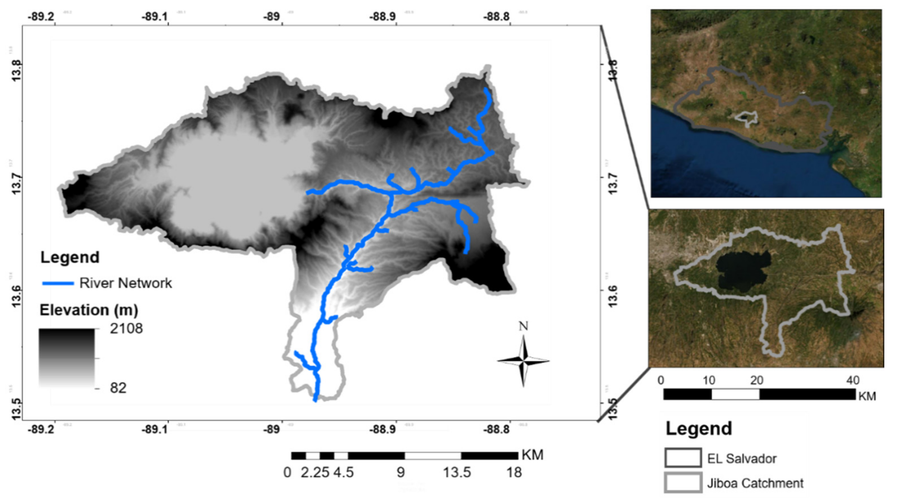
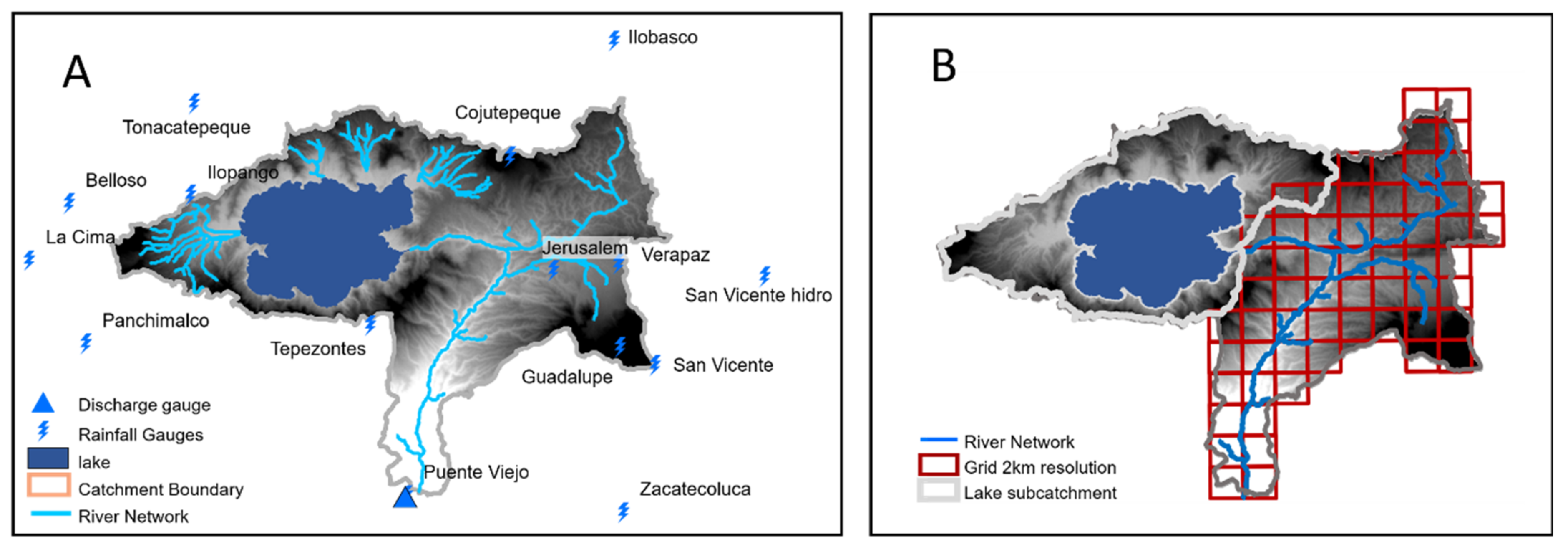
2. Case Study
3. Methods
3.1. Hydrological Model Setup
3.1.1. Hydrological Grid-Based Model “Hapi”
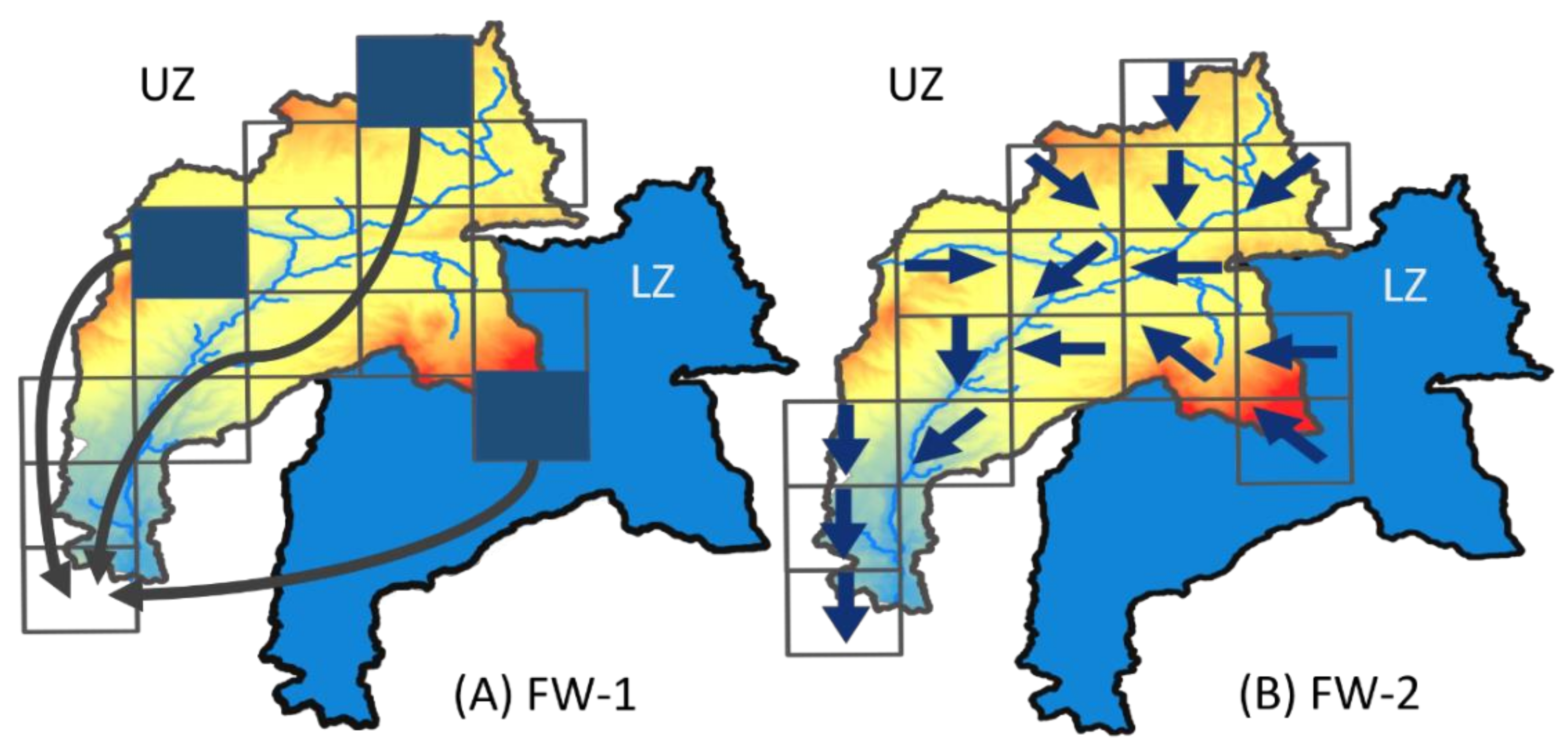
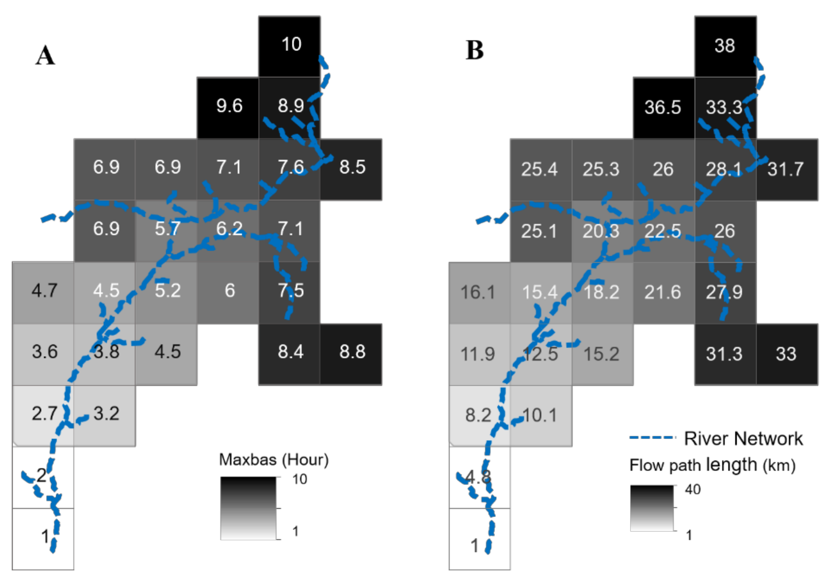
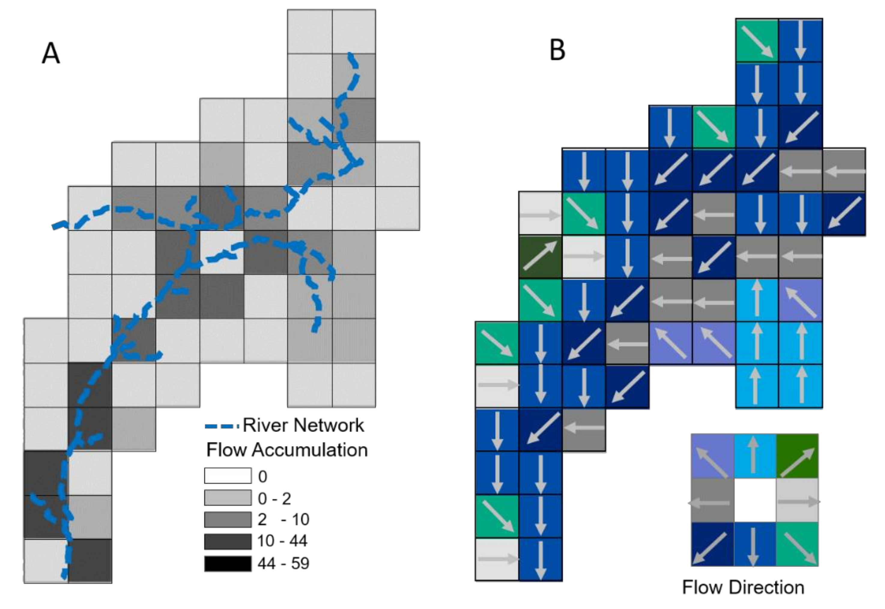
3.1.2. Spatial Discretization and Spatial Connectivity
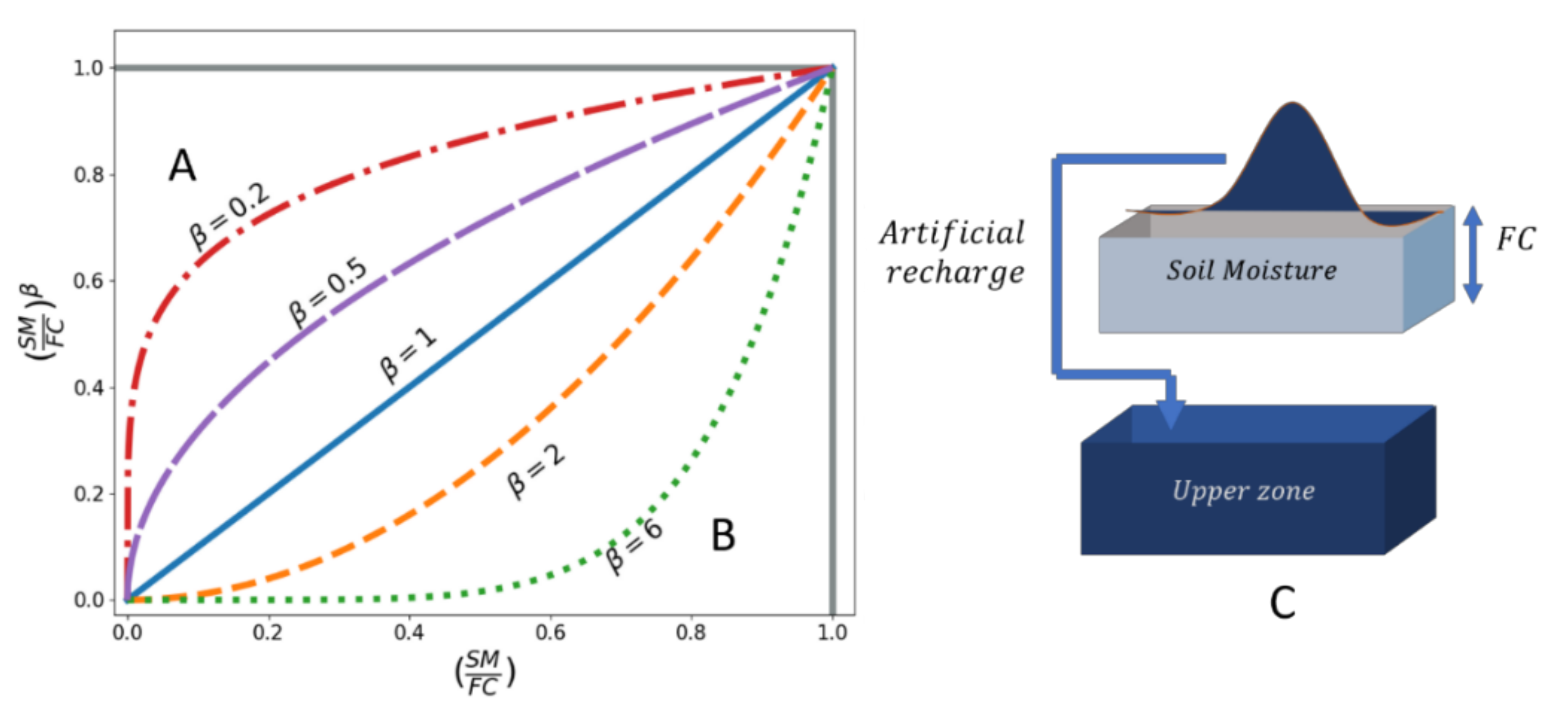
3.1.3. Model Structure
3.1.4. Model Inputs and Outputs
3.1.5. Model Parameters
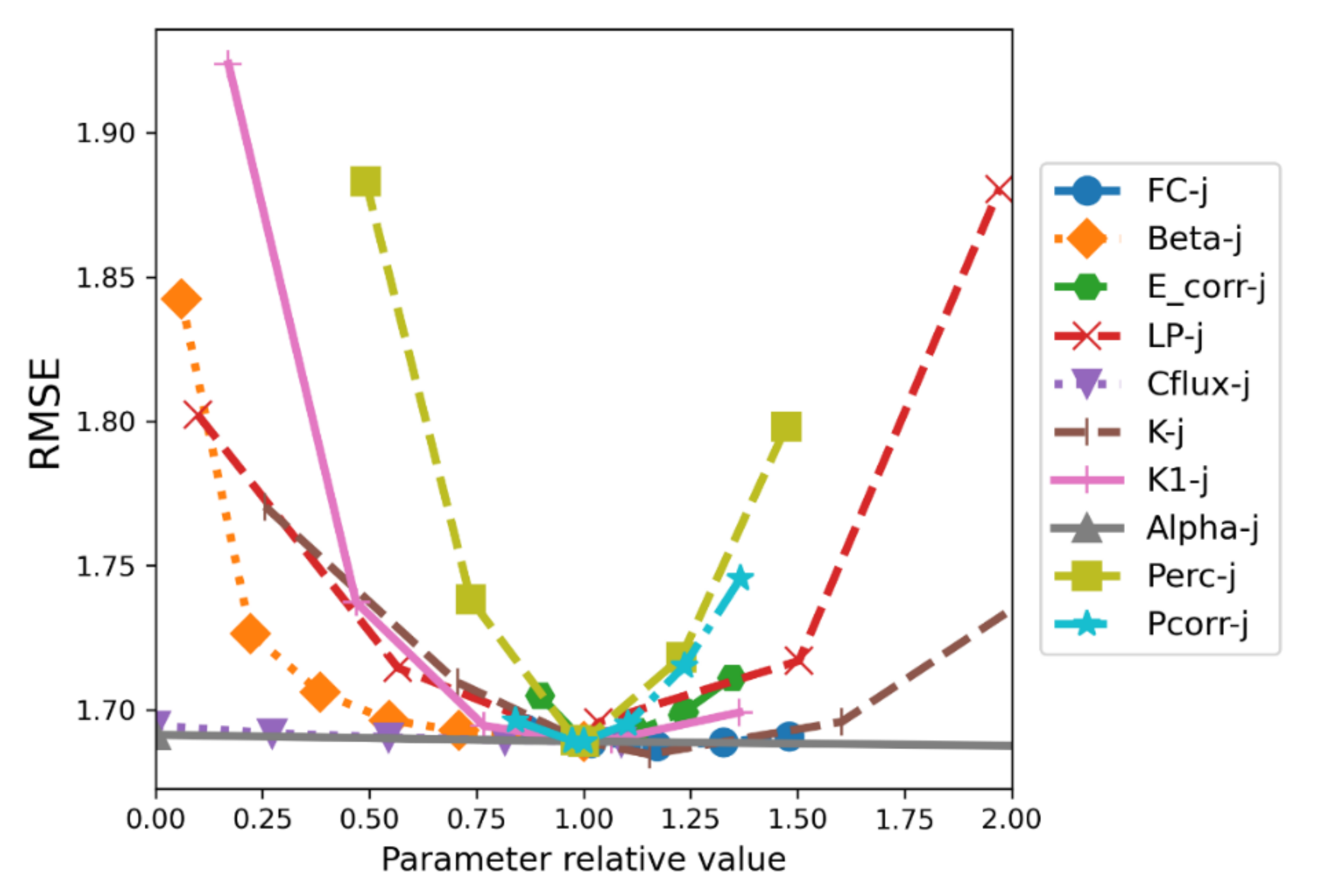
3.1.6. Parameterization Approaches
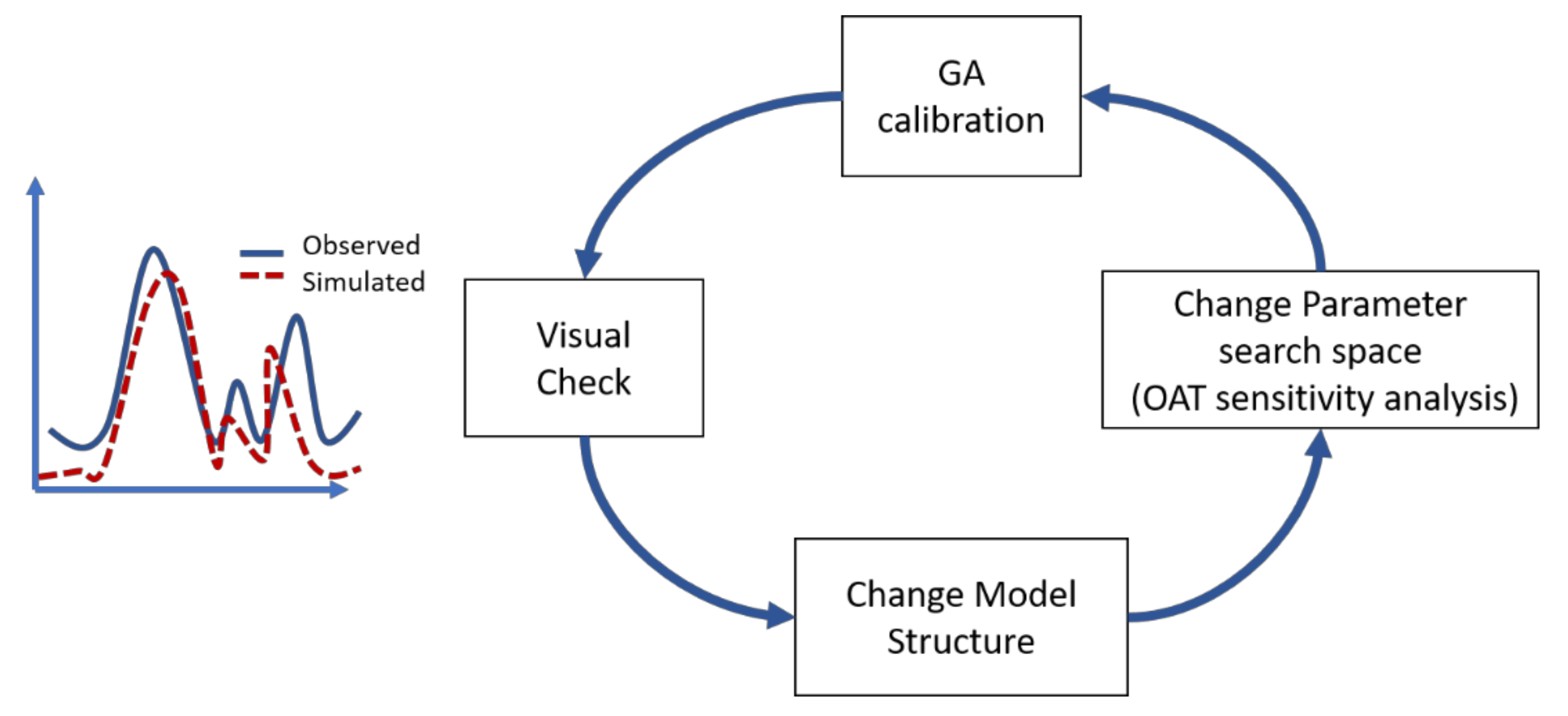
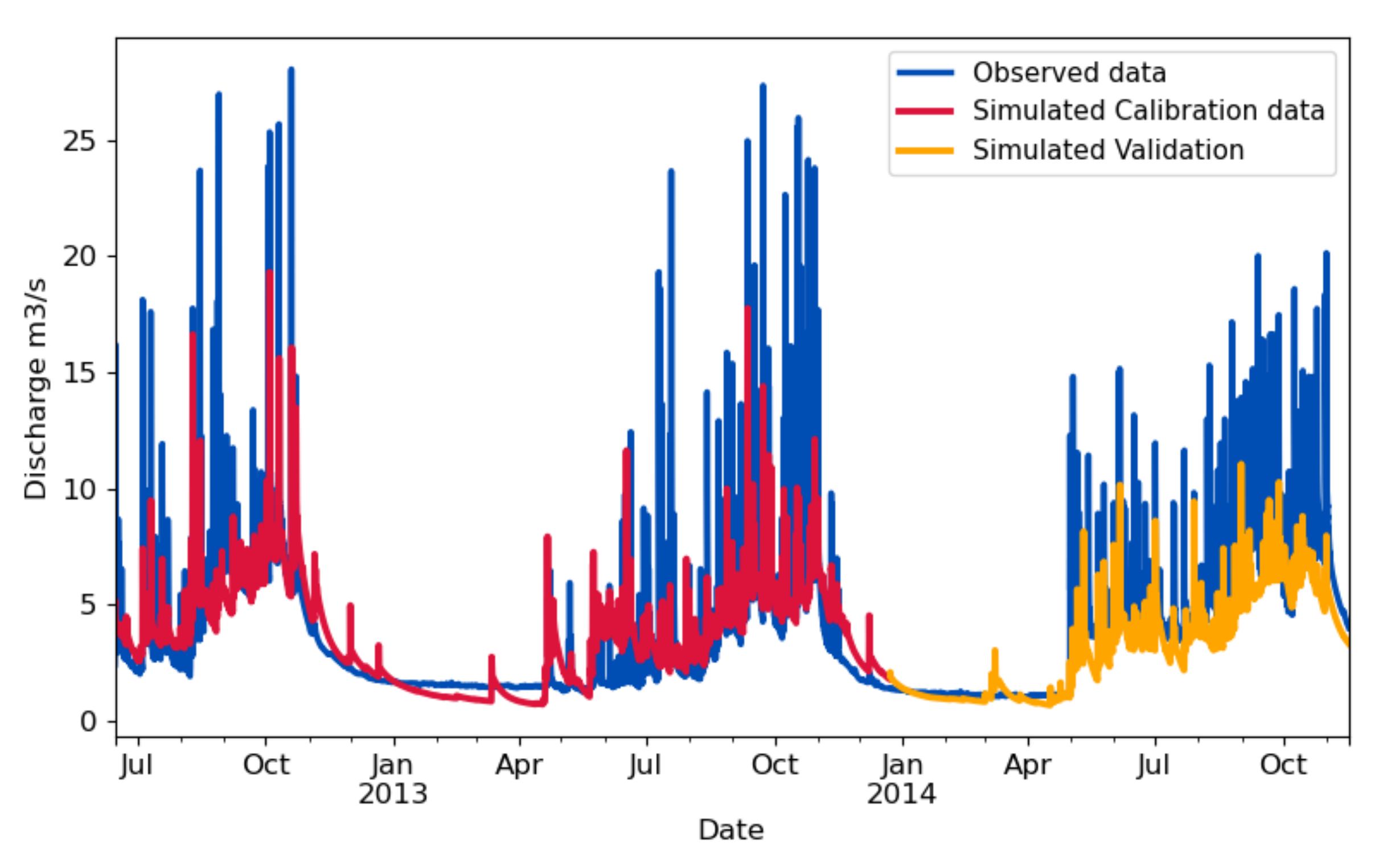
3.2. Model Calibration
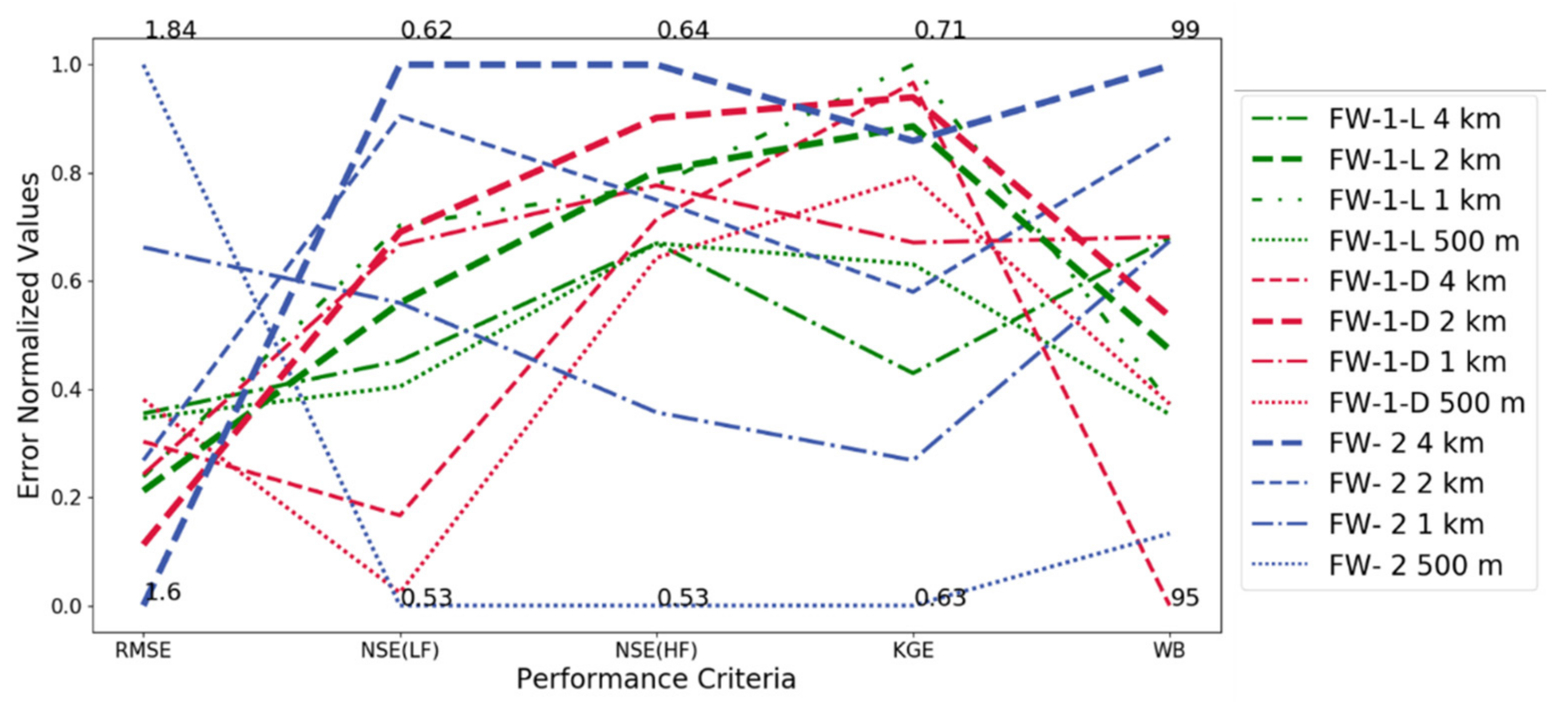
Model Performance Metrics
3.3. Data
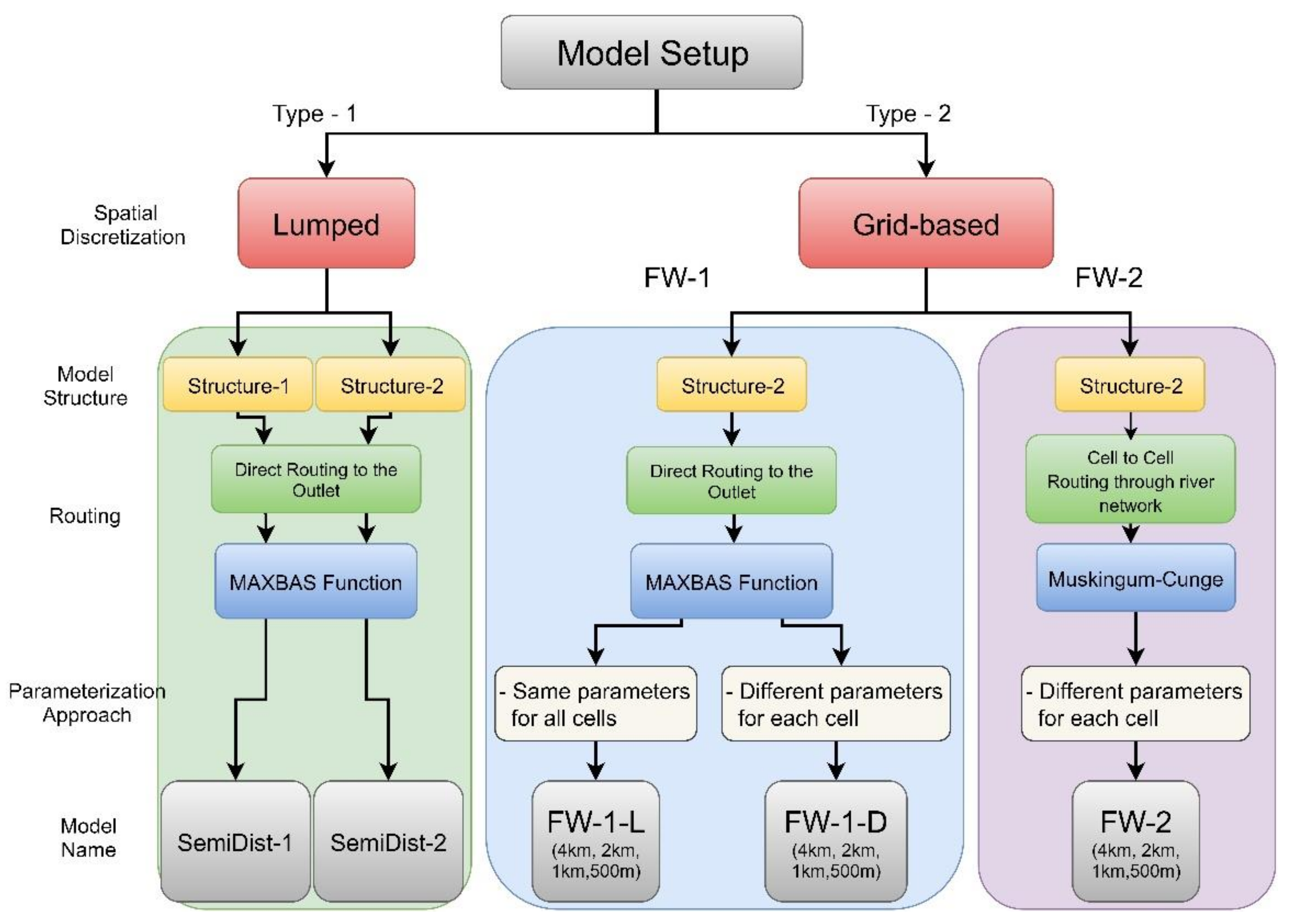
3.4. Model Setup
- Lumped model: two models are built using the lumped spatial discretization SemiDist-1 and SemiDist-2, the former is built using Model Structure-1, and the latter is built with Model Structure-2.
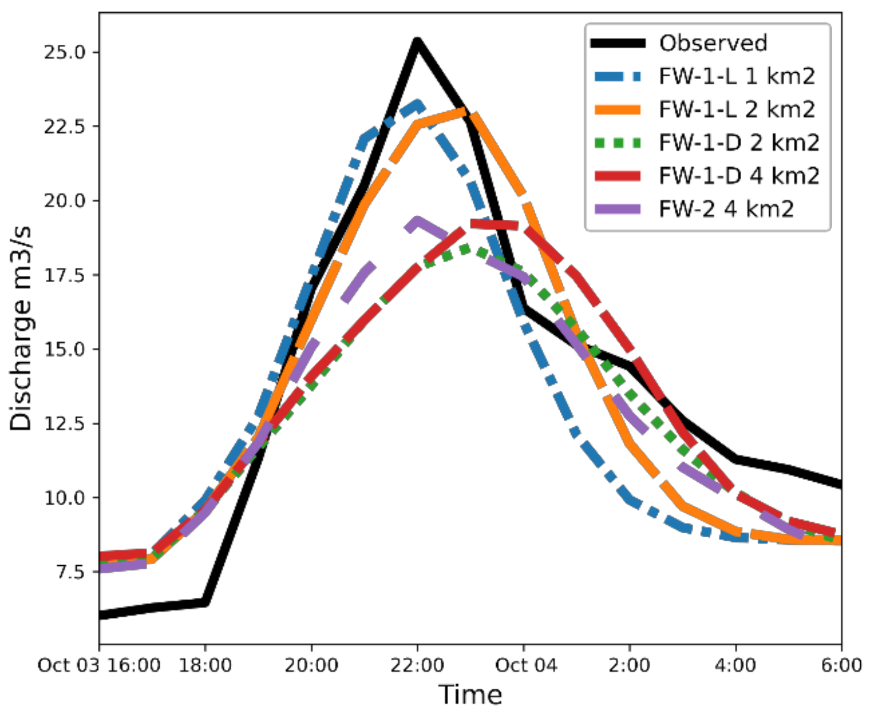
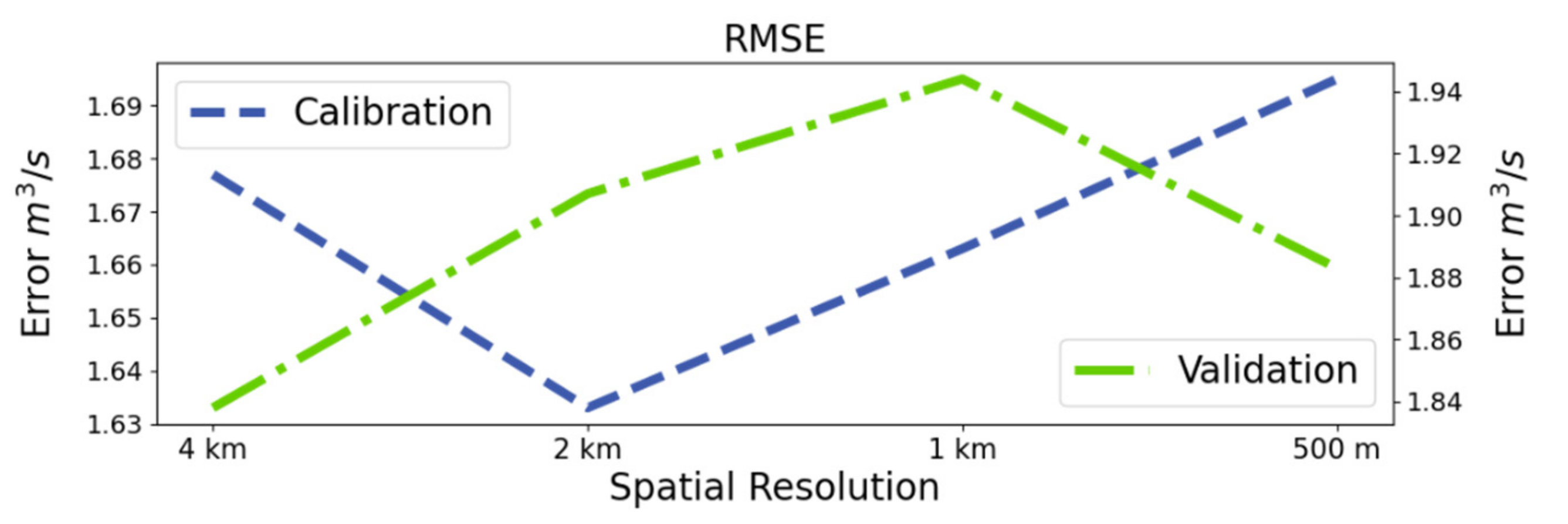
- Conceptual distributed model built with FW-1 considering lumped catchment parameters FW-1-L using different spatial resolutions (4 km, 2 km, 1 km, and 500 m).
- Conceptual distributed model built with FW-1 considering distributed catchment parameters (different parameter for each cell) FW-1-D using different spatial resolutions (4 km, 2 km,1 km, and 500 m).
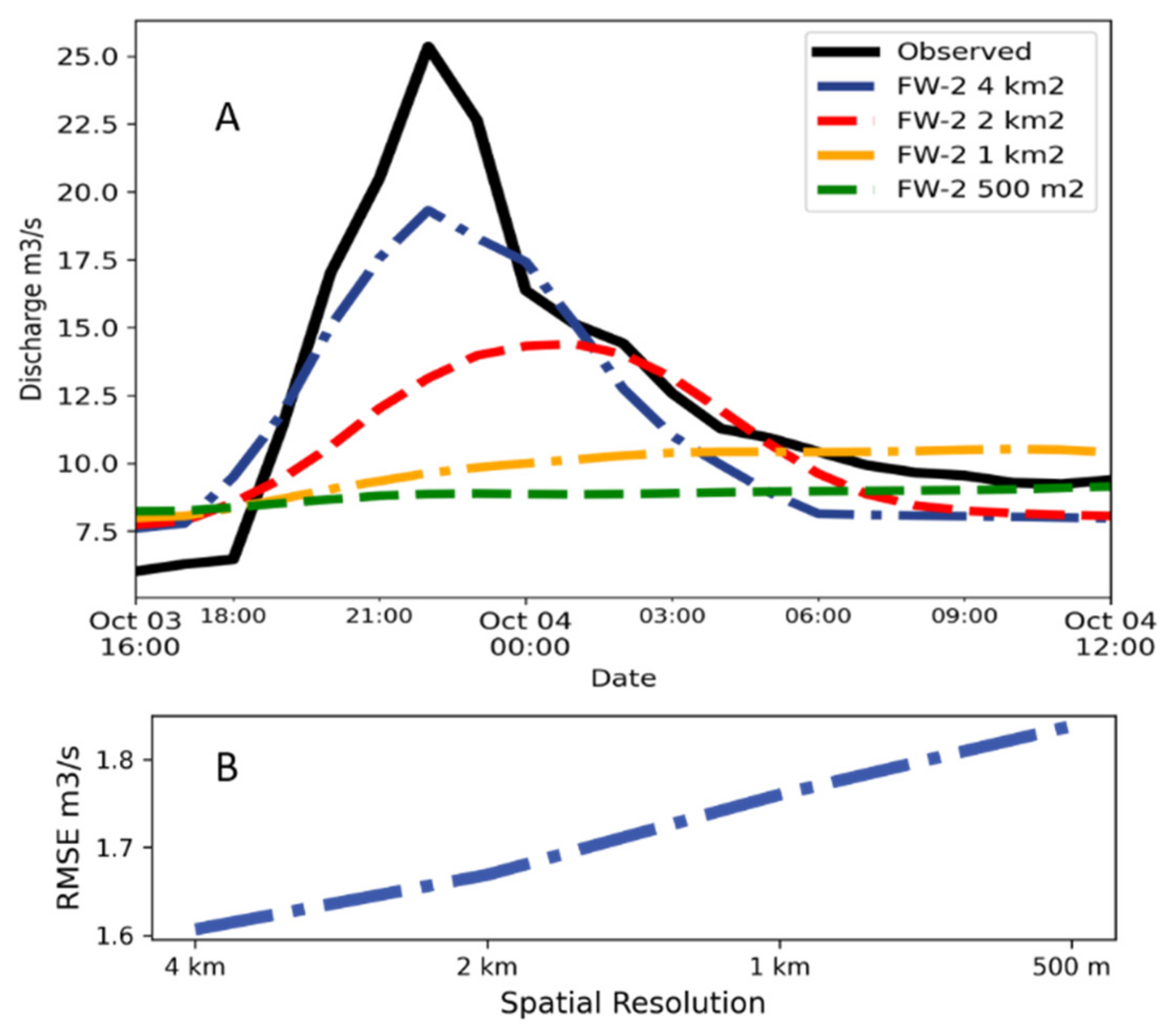
- Conceptual distributed model built with FW-2 considering distributed catchment parameters (different parameter for each cell) using different spatial resolutions (4 km, 2 km,1 km, and 500 m)
4. Results and Discussion
5. Conclusions
Author Contributions
Funding
Institutional Review Board Statement
Data Availability Statement
Acknowledgments
Conflicts of Interest
Code Availability
References
- Reggiani, P.; Rientjes, T.H.M. Flux parameterization in the representative elementary watershed approach: Application to a natural basin. Water Resour. Res. 2005, 41, 1–18. [Google Scholar] [CrossRef]
- Beven, K.; Calver, A.; Morris, E.M. The Institute of Hydrology distributed model Technical Report 98. Inst. Hydrol. Wallingford 1987, 595–626. [Google Scholar]
- Abbott, M.B.; Bathurst, J.C.; Cunge, J.A.; O’Connell, P.E.; Rasmussen, J. An introduction to the European Hydrological System—Systeme Hydrologique Europeen, “SHE”, 1: History and philosophy of a physically-based, distributed modelling system. J. Hydrol. 1986, 87, 45–59. [Google Scholar] [CrossRef]
- Bao, H.; Wang, L.; Zhang, K.; Li, Z. Application of a developed distributed hydrological model based on the mixed runoff generation model and 2D kinematic wave flow routing model for better flood forecasting. Atmos. Sci. Lett. 2017, 18, 284–293. [Google Scholar] [CrossRef]
- Abbott, M.B.; Refsgaard, J.C. The Role of Distributed Hydrological Modelling in Water Resources Management; Springer: Dordrecht, The Netherlands, 1996; Volume 22, ISBN 978-94-010-6599-3. [Google Scholar]
- Butts, M.B.; Payne, J.T.; Kristensen, M.; Madsen, H. An evaluation of the impact of model structure on hydrological modelling uncertainty for streamflow simulation. J. Hydrol. 2004, 298, 242–266. [Google Scholar] [CrossRef]
- Leavesley, G.H.; Lichty, R.W.; Troutman, B.M.; Saindon, L.G. Precipitation-runoff modeling system; user’s manual. Water Resour. Investig. Rep. 1983, 83, 207. [Google Scholar] [CrossRef]
- Iizuka, T.; Arita, K.; Yamamoto, I.; Yamamichi, S.; Yamaguchi, H.; Matsuki, T.; Sone, S.; Yabuta, H.; Miyasaka, Y.; Kato, Y. Low Temperature Recovery of Ru/(Ba, Sr)TiO3/Ru Capacitors Degraded by Forming Gas Annealing. Jpn. J. Appl. Phys. 2000, 39, 2063–2067. [Google Scholar] [CrossRef]
- Beven, K.J.; Kirkby, M.J. A physically based, variable contributing area model of basin hydrology. Hydrol. Sci. Bull. 1979, 24, 43–69. [Google Scholar] [CrossRef]
- Samaniego, L.; Kumar, R.; Attinger, S. Multiscale parameter regionalization of a grid-based hydrologic model at the mesoscale. Water Resour. Res. 2010, 46, 1–25. [Google Scholar] [CrossRef]
- Liang, X.; Lettenmaier, D.P.; Wood, E.F.; Burges, S.J. A simple hydrologically based model of land surface water and energy fluxes for general circulation models. J. Geophys. Res. Atmos. 1994, 99, 14415–14428. [Google Scholar] [CrossRef]
- Harbaugh, A.W. MODFLOW-2005: The U.S. Geological Survey Modular Ground-Water Model—the Ground-Water Flow Process; USGS: Reston, VA, USA, 2005.
- Lindström, G.; Johansson, B.; Persson, M.; Gardelin, M.; Bergström, S. Development and test of the distributed HBV-96 hydrological model. J. Hydrol. 1997, 201, 272–288. [Google Scholar] [CrossRef]
- Reggiani, P.; Hassanizadeh, S.M.; Sivapalan, M.; Gray, W.G. A unifying framework for watershed thermodynamics: Constitutive relationships. Adv. Water Resour. 1999, 23, 15–39. [Google Scholar] [CrossRef]
- Fan, Y.; Bras, R.L. On the concept of a representative elementary area in catchment runoff. Hydrol. Process. 1995, 9, 821–832. [Google Scholar] [CrossRef]
- Reggiani, P.; Sivapalan, M.; Majid Hassanizadeh, S. A unifying framework for watershed thermodynamics: Balance equations for mass, momentum, energy and entropy, and the second law of thermodynamics. Adv. Water Resour. 1998, 22, 367–398. [Google Scholar] [CrossRef]
- Dehotin, J.; Braud, I. Which spatial discretization for distributed hydrological models? Proposition of a methodology and illustration for medium to large-scale catchments. Hydrol. Earth Syst. Sci. 2008, 12, 769–796. [Google Scholar] [CrossRef]
- Refsgaard, J.C.; Storm, B.; Refsgaard, A. Recent developments of the Systeme Hydrologique Europeen (SHE) towards the MIKE SHE. IAHS Publ. 1995, 231, 427. [Google Scholar]
- Wood, E.F.; Sivapalan, M.; Beven, K.; Band, L. Effects of spatial variability and scale with implications to hydrologic modeling. J. Hydrol. 1988, 102, 29–47. [Google Scholar] [CrossRef]
- Tian, F.; Hu, H.; Lei, Z.; Sivapalan, M. Extension of the Representative Elementary Watershed approach by incorporating energy balance equations. Hydrol. Earth Syst. Sci. Discuss. 2006, 3, 427–498. [Google Scholar] [CrossRef]
- Bergström, S. Development and Application of a Conceptual Runoff Model for Scandinavian Catchments. Smhi 1976, 7, 134. [Google Scholar] [CrossRef]
- Fenicia, F.; Kavetski, D.; Savenije, H.H.G.; Pfister, L. From spatially variable streamflow to distributed hydrological models: Analysis of key modeling decisions. Water Resour. Res. 2016, 52, 954–989. [Google Scholar] [CrossRef]
- Savenije, H.H.G. HESS opinions “topography driven conceptual modelling (FLEX-Topo)”. Hydrol. Earth Syst. Sci. 2010, 14, 2681–2692. [Google Scholar] [CrossRef]
- Mayr, E.; Hagg, W.; Mayer, C.; Braun, L. Calibrating a spatially distributed conceptual hydrological model using runoff, Annual mass balance and winter mass balance. J. Hydrol. 2013, 478, 40–49. [Google Scholar] [CrossRef]
- Braun, L.N.; Aellen, M. Modelling discharge of glacierized basins assisted by direct measurements of glacier mass balance. IAHS Publ. 1990, 99–106. [Google Scholar]
- Farrag, M.; Corzo, G. MAfarrag/HAPI: HAPI. Zenodo 2021. [Google Scholar] [CrossRef]
- Schumann, A.H. Development of conceptual semi-distributed hydrological models and estimation of their parameters with the aid of GIS. Hydrol. Sci. J. 1993, 38, 519–528. [Google Scholar] [CrossRef]
- Bergström, S. The HBV model - its structure and applications. Smhi Rh 1992, 4, 35. [Google Scholar]
- Cunge, J.A. On the subject of a flood propagation computation method (Muskingum method). J. Hydraul. Res. 1969, 7, 205–230. [Google Scholar] [CrossRef]
- Johnson, D.; Miller, A. A spatially distributed hydrologic model utilizing raster data structures. Comput. Geosci. 1997, 23, 267–272. [Google Scholar] [CrossRef]
- Chaudhry, M.H. Open Channel Flow; Springer Science & Business Media: Berlin/Heidelberg, Germany, 2007; ISBN 9780387301747. [Google Scholar]
- Mishra, S.K.; Singh, V.P. Hysteresis-based flood-wave analysis using the concept of strain. Hydrol. Process. 2001, 15, 1635–1651. [Google Scholar] [CrossRef]
- Tewolde, M.H.; Smithers, J.C. Flood routing in ungauged catchments using Muskingum methods. Water SA 2006, 32, 379–388. [Google Scholar] [CrossRef]
- Rusli, S.R.; Yudianto, D.; Liu, J. Effects of temporal variability on HBV model calibration. Water Sci. Eng. 2015, 8, 291–300. [Google Scholar] [CrossRef]
- Lee, K.S.; Geem, Z.W. A new meta-heuristic algorithm for continuous engineering optimization: Harmony search theory and practice. Comput. Methods Appl. Mech. Eng. 2005, 194, 3902–3933. [Google Scholar] [CrossRef]
- Nash, E.; Sutcliffe, V. PART I-A DISCUSSION OF PRINCIPLES * The problem of determining river flows from rainfall, evaporation, and other factors, occupies a central place in the technology of applied hydrology. J. Hydrol. 1970, 10, 282–290. [Google Scholar] [CrossRef]
- Gupta, H.V.; Kling, H.; Yilmaz, K.K.; Martinez, G.F. Decomposition of the mean squared error and NSE performance criteria: Implications for improving hydrological modelling. J. Hydrol. 2009, 377, 80–91. [Google Scholar] [CrossRef]
- SNET Balance hídrico integrado y dinámico en El Salvador. Available online: https://www.snet.gob.sv/Documentos/balanceHidrico.pdf (accessed on 25 April 2021).
- Das, T.; Bárdossy, A.; Zehe, E.; He, Y. Comparison of conceptual model performance using different representations of spatial variability. J. Hydrol. 2008, 356, 106–118. [Google Scholar] [CrossRef]
- Sivapalan, M. Process complexity at hillslope scale, process simplicity at the watershed scale: Is there a connection? Hydrol. Process. 2003, 17, 1037–1041. [Google Scholar] [CrossRef]
- Dooge, J.C.I. Bringing It All Together. Hydrol. Earth Syst. Sci. 2005, 9, 3–14. [Google Scholar] [CrossRef]
- Savenije, H.H.G. Equifinality, a blessing in disguise? Hydrol. Process. 2001, 15, 2835–2838. [Google Scholar] [CrossRef]
- Gharari, S.; Hrachowitz, M.; Fenicia, F.; Savenije, H.H.G. Hydrological landscape classification: Investigating the performance of HAND based landscape classifications in a central European meso-scale catchment. Hydrol. Earth Syst. Sci. 2011, 15, 3275–3291. [Google Scholar] [CrossRef]


| Parameter Name | Description | Units | Lower Bound | Upper Bound |
|---|---|---|---|---|
| RFCF | Precipitation correction factor | - | 0.93 | 1.3 |
| FC | Maximum soil moisture storage | mm | 150 | 500 |
| Beta | Nonlinear runoff parameter | - | 0.01 | 5 |
| ETF | Evapotranspiration correction factor | - | 0.0 | 1.25 |
| LP | Limit for potential evaporation | % | 0.1 | 0.55 |
| CFLUX | Maximum capillary rate | mm/h | 0.05 | 0.55 |
| K | Upper storage coefficient | 1/h | 0.00055 | 0.008 |
| K1 | Lower storage coefficient | 1/h | 0.0035 | 0.012 |
| A | Nonlinear response parameter | - | 0 | 0.3 |
| Perc | Percolation rate | 1/h | 0.15 | 0.7 |
| Clake | Lake correction factor | % | 0.85 | 1.15 |
| Maxbas | Transfer function length | h | 1 | 7 |
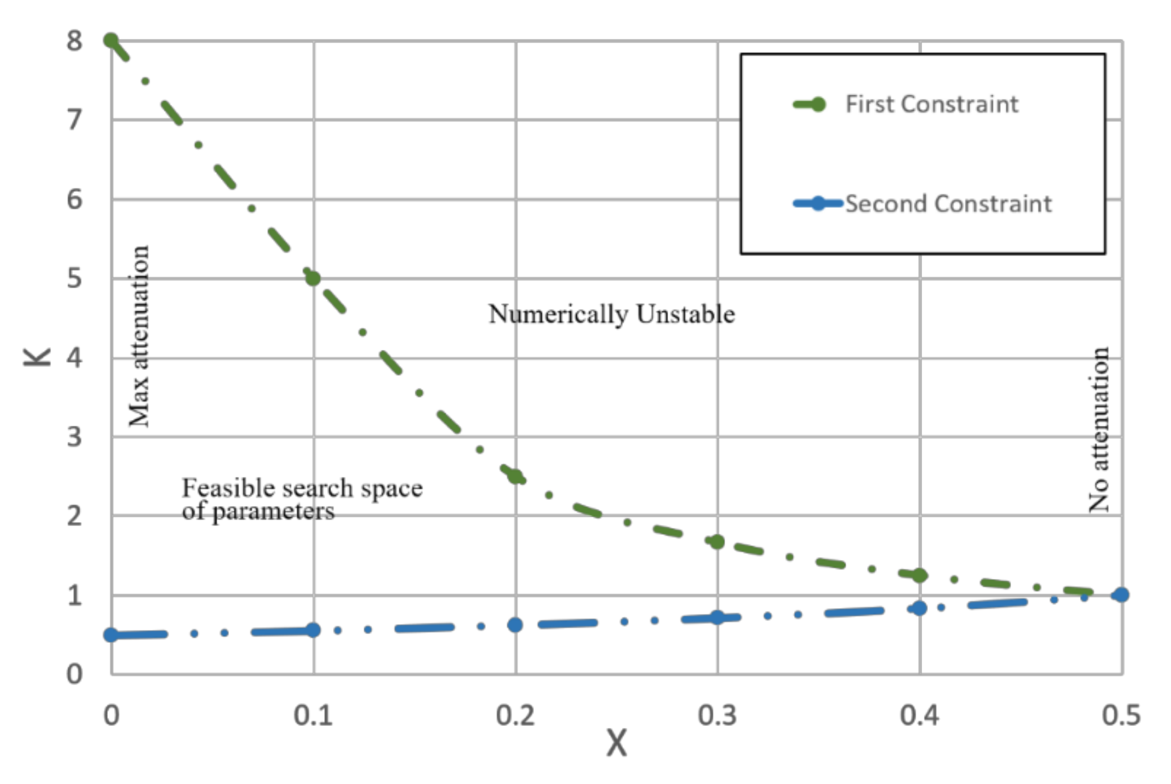
| K | Travel time | h | ||
| X | Weighting coefficient | - | 0 | 0.5 |
| Period | Ho | b | A |
|---|---|---|---|
| 05/2012–04/2013 | 0.15 | 1.89 | 13.20 |
| 05/2013–11/2013 | 0.16 | 1.90 | 13.27 |
| 11/2013–04/2014 | 0.02 | 3.00 | 15.45 |
| 05/2014–04/2015 | 0.15 | 1.25 | 13.46 |
| 05/2015–04/2016 | 0.18 | 1.73 | 20.04 |
| Model Name | Model Description | Resolution |
|---|---|---|
| SemiDist | Two models are built using the lumped spatial discretization SemiDist-1 and SemiDist-2, the former is built using Model Structure-1, and the latter is built with Model Structure-2. | Semi-distributed |
| FW-1-L | Conceptual distributed model built with FW-1 and lumped catchment parameters FW-1-L. | 4 km, 2 km, 1 km, and 500 m |
| FW-1-D | Conceptual distributed model built with FW-2 and distributed catchment parameters. | 4 km |
| FW-2 | Conceptual distributed model built with FW-2 and distributed catchment parameters. | 4 km, 2 km, 1 km, and 500 m |
| Cell Size (Km2) | RMSE | Low Flow NSE | High Flow NSE | WB | KGE | |||||
| Cal. | Val. | Cal. | Val. | Cal. | Val. | Cal. | Val. | Cal. | Cal. | |
| FW-1-L (4) | 1.69 | 1.9 | 0.57 | 0.8 | 0.6 | 0.62 | 97.8 | 73.7 | 0.66 | 0.57 |
| FW-1-L (2) | 1.65 | 1.89 | 0.58 | 0.82 | 0.61 | 0.62 | 96.7 | 74.9 | 0.69 | 0.56 |
| FW-1-L (1) | 1.66 | 1.91 | 0.59 | 0.81 | 0.61 | 0.62 | 96.2 | 74 | 0.71 | 0.56 |
| FW-1-L (500 m2) | 1.68 | 1.89 | 0.57 | 0.81 | 0.6 | 0.62 | 96.1 | 74.1 | 0.68 | 0.57 |
| FW-1-D (4) | 1.67 | 1.84 | 0.54 | 0.82 | 0.61 | 0.65 | 94.31 | 74.74 | 0.71 | 0.59 |
| FW-1-D (2) | 1.63 | 1.9 | 0.59 | 0.81 | 0.63 | 0.62 | 97.08 | 73.03 | 0.7 | 0.55 |
| FW-1-D (1) | 1.66 | 1.94 | 0.58 | 0.82 | 0.61 | 0.61 | 97.84 | 72.5 | 0.68 | 0.54 |
| FW-1-D (500 m2) | 1.69 | 1.88 | 0.53 | 0.82 | 0.6 | 0.63 | 96.24 | 73.49 | 0.69 | 0.56 |
| FW-2 (4) | 1.6 | 1.95 | 0.62 | 0.81 | 0.64 | 0.6 | 99.48 | 72.18 | 0.69 | 0.53 |
| FW-2 (2) | 1.67 | 1.98 | 0.61 | 0.8 | 0.61 | 0.58 | 98.79 | 71.54 | 0.67 | 0.53 |
| FW-2 (1) | 1.76 | 1.98 | 0.58 | 0.81 | 0.56 | 0.59 | 97.8 | 72.57 | 0.65 | 0.54 |
| FW-2 (500 m2) | 1.84 | 1.97 | 0.53 | 0.82 | 0.53 | 0.59 | 95 | 73.53 | 0.63 | 0.54 |
| SemiDist-I | 1.33 | 1.19 | 0.64 | 0.87 | 0.75 | 0.85 | 0.83 | 0.92 | 99.31 | 97.45 |
| SemiDist-II | 1.65 | 1.72 | 0.59 | 0.82 | 0.62 | 0.69 | 0.71 | 0.65 | 99.49 | 85.1 |
| Model | RFCF | FC | Β | E_corr | LP (%) | CFLUX (mm/h) | K (1/h) | K1 (1/h) | A | Perc (mm/h) | MAX-BAS |
|---|---|---|---|---|---|---|---|---|---|---|---|
| SemiDist-1 | 1 | 547.7 | 0.0443 | 0.589 | 0.071 | 1.421 | 0.0053 | 0.0063 | 0.096 | 0.304 | 3 |
| SemiDist-2 | 1.07 | 359.3 | 4.19 | 0.942 | 0.045 | 0.333 | 0.0043 | 0.0062 | 0.020 | 0.438 | 5 |
Publisher’s Note: MDPI stays neutral with regard to jurisdictional claims in published maps and institutional affiliations. |
© 2021 by the authors. Licensee MDPI, Basel, Switzerland. This article is an open access article distributed under the terms and conditions of the Creative Commons Attribution (CC BY) license (https://creativecommons.org/licenses/by/4.0/).
Share and Cite
Farrag, M.; Perez, G.C.; Solomatine, D. Spatio-Temporal Hydrological Model Structure and Parametrization Analysis. J. Mar. Sci. Eng. 2021, 9, 467. https://doi.org/10.3390/jmse9050467
Farrag M, Perez GC, Solomatine D. Spatio-Temporal Hydrological Model Structure and Parametrization Analysis. Journal of Marine Science and Engineering. 2021; 9(5):467. https://doi.org/10.3390/jmse9050467
Chicago/Turabian StyleFarrag, Mostafa, Gerald Corzo Perez, and Dimitri Solomatine. 2021. "Spatio-Temporal Hydrological Model Structure and Parametrization Analysis" Journal of Marine Science and Engineering 9, no. 5: 467. https://doi.org/10.3390/jmse9050467
APA StyleFarrag, M., Perez, G. C., & Solomatine, D. (2021). Spatio-Temporal Hydrological Model Structure and Parametrization Analysis. Journal of Marine Science and Engineering, 9(5), 467. https://doi.org/10.3390/jmse9050467