Rapid Assessment of Tsunami Offshore Propagation and Inundation with D-FLOW Flexible Mesh and SFINCS for the 2011 Tōhoku Tsunami in Japan

Abstract

This study demonstrates the skills of D-FLOW Flexible Mesh (FM) and SFINCS (Super-Fast INundation of CoastS) in combination with the Delft Dashboard Tsunami Toolbox to numerically simulate tsunami offshore propagation and inundation based on the example of the 2011 Tōhoku tsunami in Japan. Caused by a megathrust earthquake, this is one of the most severe tsunami events in recent history, resulting in vast inundation and devastation of the Japanese coast. The comparison of the simulated with the measured offshore water levels at four DART buoys located in the north-western Pacific Ocean shows that especially the FM but also the SFINCS model accurately reproduce the observed tsunami propagation. The inundation observed at the Sendai coast is well reproduced by both models. All in all, the model outcomes are consistent with the findings gained in earlier simulation studies. Depending on the specific needs of future tsunami simulations, different possibilities for the application of both models are conceivable: (i) the exclusive use of FM to achieve high accuracy of the tsunami offshore propagation, with the option to use an all-in-one model domain (no nesting required) and to add tsunami sediment dynamics, (ii) the combined use of FM for the accurate simulation of the tsunami propagation and of SFINCS for the accurate and time efficient simulation of the onshore inundation and (iii) the exclusive use of SFINCS to get a reliable picture of the tsunami propagation and accurate results for the onshore inundation within seconds of computational time. This manuscript demonstrates the suitability of FM and SFINCS for the rapid and reliable assessment of tsunami propagation and inundation and discusses use cases of the three model combinations that form an important base for tsunami risk management.

1. Introduction

The concentration of the world’s population, industry and tourism in coastal areas make tsunamis a major risk to today’s society. Events like the 2004 Indian Ocean tsunami or the 2011 Tōhoku tsunami in Japan have demonstrated the devastating power of tsunamis in coastal areas, resulting in huge human, ecological and economical losses. Prediction of future tsunami inundation is the very essence of tsunami risk management. In the long-term it facilitates sustainable spatial planning and the construction of defence structures; in the short-term it allows effective evacuation and rescue of the coastal population in the inundation area.

While storm surge forecast techniques are highly advanced, prediction of tsunami impact is particularly challenging owing to the sudden and infrequent nature of this phenomenon. Besides information on past tsunami events, e.g., [1,2,3], numerical hydrodynamic models are an important tool for the assessment of tsunami hazards in both the long- and short-term. Modern computational power allows for the simulation of tsunami events with numerical models within seconds to hours computational time (i.e., shorter than real-time) in high spatial and temporal resolution. In this study, we investigate the capability of two numerical hydrodynamic models, i.e., the D-FLOW Flexible Mesh (FM) module [4,5] and SFINCS (Super-Fast INundation of CoastS; [6]), in combination with the Delft Dashboard (DDB) Tsunami Toolbox [7], to assess rapidly and reliably the offshore propagation and inundation associated with the 2011 Tōhoku tsunami in Japan.

FM is the derivative of Delft3D-FLOW version 4 (D3D)—a fully validated program module to simulate both tsunami offshore propagation and inundation, including sediment transport [8]. D3D has been successfully employed for 1-D [9], 2-D [10,11,12,13,14,15,16,17] and 3-D tsunami simulations [8,18,19,20,21]. Accordingly, SFINCS is a validated model for the simulation of compound flooding in an accurate and, at the same time, computationally highly efficient way [6,22]. The model is particularly suited for the simulation of water levels in the swash zone and onshore. Finally, the DDB Tsunami Toolbox allows for the determination of the initial tsunami wave, based on the focal mechanism of an earthquake and was successfully applied to perform simulations of the 2011 Tōhoku tsunami with a D3D model [7].

The 2011 Tōhoku tsunami, used as test case in this study, is one of the most severe tsunami events of the recent history. The tsunami caused vast inundation and devastation of the north-east coast of Honshū Island, i.e., the main island of Japan (Figure 1A). Altogether, more than 20,000 people fell victim to this event [23,24]. The estimated total financial damage associated with the tsunami and triggering earthquake amounts to almost $335 billion for the year 2011 only [25], making it the costliest natural disaster ever recorded. The tsunami is having long lasting consequences for the area, especially due to the radioactive contamination associated with nuclear meltdowns after the flooding of the Fukushima II nuclear power plant located south of the Sendai coast (Figure 1B).

The Tōhoku tsunami was caused by a megathrust earthquake with a magnitude of M_w = 9.1 about 130 km offshore Sendai in north-eastern Japan on 11 March 2011 ([26]; Figure 1A). Tsunami formation was favoured by the shallow focus depth (approximately 30 km) and the considerable vertical seafloor displacement by up to 9.7 m [27,28,29]. The latter was associated with a comparatively small rupture area of almost 45,000 km² with highly concentrated slip [30]. Moreover, the rupture velocity of the source mechanism was comparatively low (1.5 km s⁻¹ to 2 km s⁻¹; [26]). This altogether caused the generation of high-amplitude tsunami waves with maximum run-up heights of about 39 m and a maximum inland penetration of nearly 5 km at the north-east coast of Honshū island [23,24,31].

The objective of the current study is to demonstrate the skills of D-FLOW Flexible Mesh and SFINCS in combination with the Delft Dashboard Tsunami Toolbox to simulate tsunami offshore propagation and inundation as a valuable base for rapid and reliable assessment of tsunami hazards. For this objective, we use the test case of the 2011 Tōhoku tsunami and the study by [7] as basis and (i) derive the initial water level displacement associated with the crust movement during the Tōhoku earthquake, (ii) setup an all-in-one propagation and inundation FM model covering the north-western Pacific Ocean including the Sendai coast in high resolution, (iii) setup a separate propagation and inundation SFINCS model and (iv) validate the simulated tsunami propagation and inundation at the Sendai coast against measurements and compare the results with earlier studies including [7]. Finally, we discuss the benefits of the different model configurations for the simulation of tsunami propagation and inundation and provide use cases for their application.

2. Materials and Methods

In this study, we apply the D-FLOW Flexible Mesh module and SFINCS to simulate the 2011 Tōhoku tsunami. Moreover, the D3D reference model—a further developed model based on [7]—is applied for a direct comparison with the FM and SFINCS simulation results. In total, four different model configurations are applied in order to test the ability of each model to reproduce both the observed (i) tsunami offshore propagation and (ii) the associated inundation (cf. Figure 2):

(1)

Based on an all-in-one FM model, both the tsunami propagation in the north-eastern Pacific and inundation at the coast of the Sendai Bay are simulated within a single model domain (no nesting required; Figure 2A).

(2)

Based on the all-in-one FM model, the tsunami propagation is simulated, while the inundation is simulated with a nested SFINCS model (a similar approach as needed for the D3D reference model; Figure 2B), which is forced with hydrodynamic boundary conditions derived from the all-in-one FM model.

(3)

Same as (2) but the nested SFINCS model is forced with hydrodynamic boundary conditions derived from an overall SFINCS model in order to also test the ability of SFINCS to reproduce deep-water tsunami wave propagation (Figure 2B).

(4)

The D3D reference model is a further developed model based on [7] (separated in an overall and nested model; Figure 2B), using updated topography data, bottom roughness and initial tsunami water levels as applied in the other models of this study (Section 2.1).

In the case of both, the SFINCS and D3D nested models (i.e., model configurations (2)–(4)), the coupling with the overall models is one-way, which means that the solutions of the nested models do not propagate back into the overall models.

For the validation of the simulated tsunami propagation, we compare simulated with measured water level time-series at four offshore DART (Deep-ocean Assessment and Reporting Tsunami) buoys located in the north-western Pacific Ocean (Figure 1A; [32]). The simulated maximum inundation water levels (as derived from Fourier analyses) are compared with the inundation levels derived from 620 observed high-water marks (corrected for tidal elevations) at the coast of the Sendai Bay according to [23,33]. For a quantitative comparison of the simulated and measured offshore and inundation water levels, the statistical parameters RMSE (root-mean-square error), bias and SCI (scatter index) are determined.

2.1. Delft3D-FLOW Reference Model

The D3D reference model (version 6.03.00.65936M) is a further developed model based on [7] and comprises a separate overall and nested model (Figure 2B). The overall model covers the north-western Pacific Ocean (Figure 1A) with a resolution of about 0.05° (approximately 4400 m by 5600 m offshore the Sendai Bay) and a total number of (rectangular) computational grid cells of 472,888. The nested model covers the wider Sendai Bay and adjacent coast (Figure 1B) with a resolution of 68 m by 86 m and 400,000 (rectangular) grid cells.

Compared to the study of [7], improvements were made in the model schematisation regarding the onshore elevation data, off- and onshore bottom roughness and the initial displacement of the water column:

• In order to increase the accuracy of the model’s topography, the onshore elevation data were changed from SRTM (Shuttle Radar Topography Mission; [34]) data to more accurate ALOS (Advanced Land Observing Satellite, [35]) data with a spatial resolution of 30 m. The ALOS data were referenced to local mean sea level (MSL) using the DTU10 Mean Dynamic Topography dataset [36]. The ALOS topography data were merged with GEBCO (General Bathymetric Chart of the Oceans) bathymetry data [37] as used by [7].
• It was found that to simulate the maximum onshore water levels more accurately, the bottom roughness had to be increased, as suggested by [38] for the application of depth-integrated tsunami inundation models. Based on this and on several tests with different bottom roughness fields in the FM model (Section 2.2), we therefore applied a Manning’s n coefficient of 0.025 s m^−1/3 offshore and a higher value of 0.1 s m^−1/3 onshore in the D3D, FM and SFINCS models. These values yielded the best reproduction of the observed water levels and inland penetration at the coast of the Sendai Bay over the three applied models.
• Finally, the initial displacement of the water column was calculated more accurately based on fault segment data by [28]. These data contain information on the location, depth, slip, rake, strike and dip for 190 separate fault segments. The total length of the applied fault line amounts to approximately 500 km [28]. The fault segment data were processed using the DDB Tsunami Toolbox [7]. This toolbox makes use of a set of analytical expressions by [39] (referred to as the Okada model) to model fluid surface deformation fields (in two dimensions) caused by seafloor displacement during earthquakes. Based on this input, the DDB tool generates a spatially varying initial water level field interpolated on the computational grid/mesh of the D3D/SFINCS/FM models, representing the initial tsunami wave. The use of the fault segment data by [28] results in a steeper and higher initial tsunami wave with a shorter wave period compared to [7].

The simulation time of the D3D reference as well as of the FM and SFINCS models amounts to 6 h 15 min and starts at the time when the earthquake occurred (05:46 UTC on 11 March 2011) with the initial displacement of the water column associated with the crust movement during the earthquake. Owing to the steeper initial tsunami wave applied in the updated model, it was necessary to apply a smaller time step for the overall model of 3.75 s in order to guarantee numerical stability. All other model settings including the boundary conditions and physical and numerical parameters are the same as described by [7].

2.2. D-FLOW Flexible Mesh Model

The D-FLOW Flexible Mesh module as part of the Delft3D Flexible Mesh suite solves the non-linear shallow water equations of unsteady flow and transport phenomena derived from the three-dimensional Navier Stokes equations for incompressible free surface flow [4,5]. The module is designed for flow phenomena where the horizontal spatial and temporal scales are much larger than the vertical scales, such as tidal waves, storm surges or (weakly to non-dispersive) tsunamis. D-FLOW Flexible Mesh can be applied in two-dimensional (depth-averaged) or three-dimensional mode, the latter based on the use of vertical layers (not fully three-dimensional). As the water density in the oceans can approximately be regarded as vertically homogeneous, the two-dimensional, depth-averaged calculation mode is appropriate for tsunami simulations conducted here.

The FM model (version 2.09.09.64406) is in principle based on the D3D reference model by [7] but uses an all-in-one computational mesh. This allows the simulation of both the tsunami propagation and inundation in a single model run without nesting. The FM model has the same domain and offshore mesh resolution as the D3D model (Figure 1A). Towards the coast of the Sendai Bay, the mesh resolution stepwise increases to a maximum resolution of 68 m by 86 m (Figure 1B and Figure 2A), which is equal to the resolution of the nested D3D model. In total, the mesh comprises 1,195,114 nodes. The mesh is generally based on rectangular cells and uses triangular cells for connecting rectangular cells with different resolution. The model’s bathymetry and topography as well as off- and onshore Manning’s n bottom roughness coefficients are the same as in the D3D reference model (Section 2.1). Following the approach by [7], all offshore model boundaries are open hydrodynamic boundaries based on the Riemann invariant, in order to avoid any unintended wave reflection, cf. [5,40].

For the model calibration, we varied the maximum time step (Dtmax 1 s–30 s), the value for the compromise in explicit/implicit time integration (Theta0 0.5–0.55) and the bottom roughness fields (Manning’s n roughness coefficient between 0.018 s m^−1/3 and 0.025 s m^−1/3 offshore and between 0.03 s m^−1/3 and 0.1 s m^−1/3 onshore; cf. Section 2.1). The final chosen Dtmax is 30 s in combination with a Theta0 of 0.54, which resulted in the best match with the measured water levels at the four DART buoys.

2.3. SFINCS Model

SFINCS has been established as an alternative approach to advanced process-based models in order to optimise computational demand and the required physics. SFINCS uses an efficient numerical scheme to solve a set of simplified depth-averaged shallow-water equations in which horizontal viscosity is neglected (i.e., the linear shallow water equations). Moreover, Coriolis as well as advection terms can be turned off, resulting in the local inertial equations. The SFINCS model was successfully applied to reproduce the wave-driven flooding of the village of Hernani in the Philippines during typhoon Haiyan in 2013 [6]. In this study, we apply SFINCS to model onshore inundation forced by the FM model and also—for the first time—to simulate offshore tsunami propagation.

The computational grid of the overall SFINCS model (code revision 226) has a similar extent to that of the D3D/FM models (Figure 1A) and has a uniform spatial resolution of 1000 m by 1000 m. The resolution is needed to be higher than the coarsest offshore resolution of the FM mesh in order to simulate the tsunami wave propagation into the Sendai Bay in sufficient detail. The overall model grid counts 9,452,582 cells and is forced with the same initial water displacement as the D3D/FM models.

The nested SFINCS model grid covers the inner Sendai Bay, with a maximum offshore extent roughly at the −30 m water depth contour (Figure 1B). The nested model grid counts 168,966 active cells and has a uniform resolution of 68 m by 86 m (i.e., identical to the nested D3D model and the high-resolution area of the FM model). The hydrodynamic boundary conditions of the nested SFINCS model were directly derived from the output at various observations points in (i) the FM model and (ii) the overall SFINCS model, which are exactly located at each cell along the open boundary of the nested SFINCS model. For this, the water level time-series computed by the overall FM/SFINCS models for each observation point during the simulation time of 6 h 15 min was separated into incoming and outgoing wave components and only the incoming tsunami wave was applied at the boundaries of the nested SFINCS model. The nested SFINCS model is forced with a slowly and a fast-varying component using a 10-min moving mean using the method of [41] as described in [6], to keep the front of the nested tsunami wave as steep as forced.

The SFINCS models use the same bathymetry and topography data as well as the same off- and onshore Manning’s n bottom roughness coefficients as the D3D reference and FM models (Section 2.1 and Section 2.2). The nested SFINCS model is applied with default settings with an increased theta value (no advection, no Coriolis, alpha = 0.75, theta = 0.99). For the offshore propagation, this is a first-time application and calibration tests showed that best results are obtained by using the new subgrid version of SFINCS [22], together with modified numerical settings to avoid too strong reflections at the coast and too much smoothing of the tsunami wave (advection turned on, Coriolis on, alpha = 0.55, theta = 0.99, advlim = 5, spinup = 0). Here, Coriolis is included based on a constant latitude. The SFINCS models are run on a NVIDIA V100 tensor core GPU (Graphics Processing Unit) for maximum computational speed-up.

3. Results

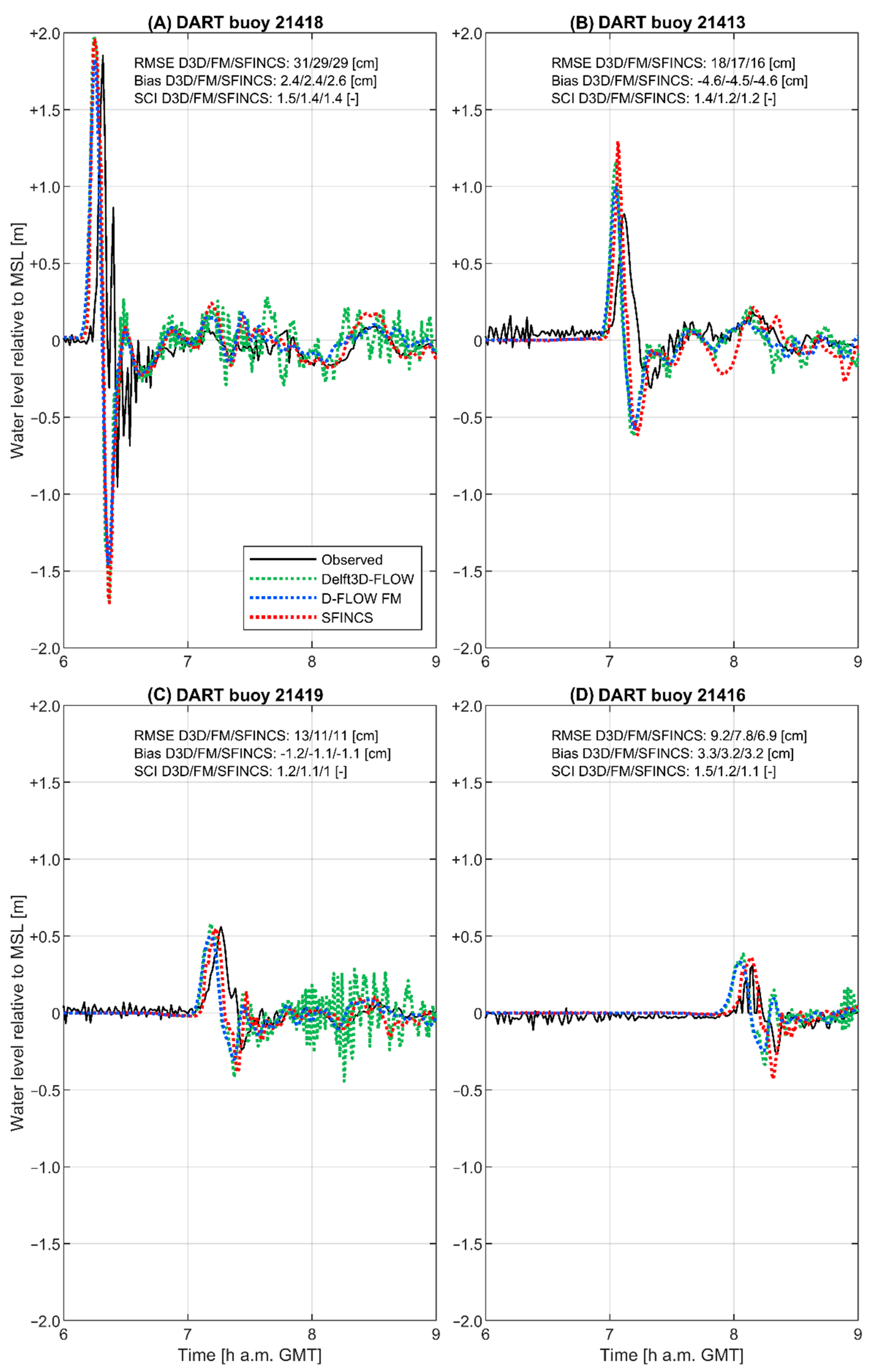
3.1. Tsunami Propagation

Figure 3A displays the maximum water levels above MSL simulated with the FM model for the north-western Pacific Ocean. The maximum (initial) water levels along the rupture zone amount to more than 12 m above MSL resulting in tsunami wave amplitudes of more than 10 m above MSL along most parts of the Honshū coast, where the first wave crest arrives about 25 min after the earthquake occurred. A clear elongated beaming of the tsunami wave energy in a south-eastern (seaward) and north-western (landward) direction, i.e., at a right angle to the fault line, can be observed. This beaming is favoured by the considerable length of the fault line of about 500 km, cf. [3,42]. The maximum water levels along the eastern model boundary, almost 2000 km distant from the rupture zone, still exceed 1.6 m above MSL. The islands chains to the north-east and south-west of Japan’s main islands form a clear barrier against tsunami propagation. In the Sendai Bay, the simulated maximum water levels before landfall exceed 12 m above MSL (Figure 3B).

Figure 4A indicates a similar order and spatial pattern of simulated maximum water levels in the north-western Pacific Ocean for the case of the overall SFINCS model. However, the beaming of tsunami wave energy is more pronounced resulting in higher water levels along the main axis of tsunami propagation. In the Sendai Bay, the simulated maximum water levels are slightly below the predictions by the FM model (Figure 4B).

In Figure 5, the water level time-series as simulated with the FM model are compared with the water level time-series measured at four DART buoys in the north-western Pacific Ocean (see Figure 3 for the locations). The measured water level time-series at all four DART buoys (black solid lines in Figure 5) indicate an asymmetrical leading-elevation N-wave [3,43] with a clearly larger wave crest than wave trough. The absolute peak at each DART buoy is reached during the first crest, followed by a comparatively small wave trough and ongoing minor water level oscillations. DART buoys 21418 and 21413 are located in the beam of the tsunami wave energy (Figure 3A) and therefore show the highest measured water levels of up to 1.9 m and 0.8 m above MSL respectively. DART buoys 21419 and 21416 are located outside the beam further north-eastward and therefore show smaller peaks in the measured water levels of about 0.6 m and 0.3 m above MSL respectively.

At DART buoys 21418 and 21413 located in the beam of the tsunami, the amplitude, period and timing of the entire tsunami wave train are generally well reproduced by the FM model (blue dotted lines in Figure 5A,B), although the first wave crest and trough are slightly shifted at both buoys and the amplitude of the first wave trough is overestimated. On average, the model slightly over-/underestimates the measured water levels by about 2.4 cm/4.5 cm at DART buoys 21418/21413. The corresponding RMSE values of 29 cm and 17 cm, respectively, indicate that the statistical dispersion of the simulated water levels is larger than of the measured water levels. This is particularly due to the time shift observed for the first wave crest and trough.

At DART buoys 21419 and 21416 located outside the beam of the tsunami (Figure 5C,D), the measured water levels are even better reproduced by the model, although a slight shift in the timing can still be observed. The lower values of the RMSE of 11 cm and 7.8 cm respectively indicate that the statistical dispersion of the simulated water levels compared to the measured water levels is generally lower than at DART buoys 21418 and 21413.

The simulation results of the SFINCS model show that—although the software is not developed for deep-water wave propagation—the model is able to reproduce the measured tsunami water levels at all four DART buoys (red dotted lines in Figure 5). While the timing of the first wave crest and trough is better at almost all DART buoys in the SFINCS model compared to the FM model, the amplitudes are clearly overestimated, especially at DART buoys 21418 and 21413. Moreover, the following water level oscillations in the SFINCS model show a larger discrepancy with the measurements at all buoys. Nevertheless, the values of the RMSE, bias and SCI are very similar to those of the FM model.

A comparison of the FM and SFINCS model results with those of the D3D reference model (green dotted lines in Figure 5) demonstrates that the D3D model can capture the first wave crest and trough but—despite the reduced time step (cf. Section 2.1)—is less stable afterwards. The latter results in higher RMSE values, especially at DART buoys 21419 and 21416.

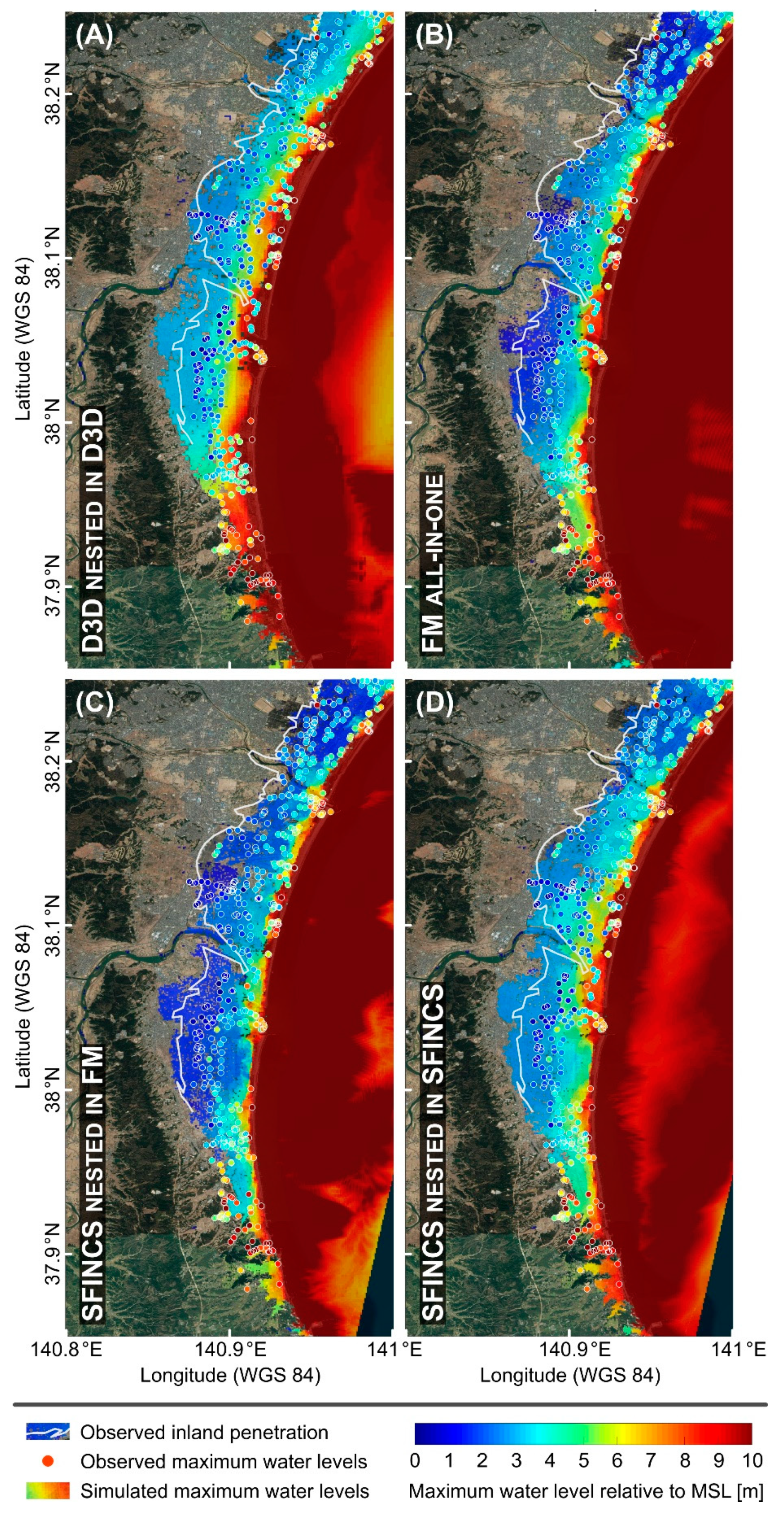
3.2. Tsunami Inundation

After a simulation time of 1 h 5 min (i.e., 1 h 5 min after the earthquake has occurred) in the applied models, the main tsunami crest hits the coast of the Sendai Bay. The resulting simulated maximum water levels at the Sendai coast are displayed in Figure 6, which, for comparison, also shows the inland penetration (i.e., the maximum onshore inundation extent) as observed in the field and the maximum water levels as derived from 620 observed high-water marks (cf. Section 2).

The observed inland penetration, which is strongly controlled by the topography of the study area (low lying delta bounded by mountains and river valleys), is well reproduced by the FM model (Figure 6B). The simulated maximum water levels show a reasonable match with the observed high-water marks. On average, the FM model overestimates the maximum water levels by about 1.2 m and shows a larger dispersion than the observations (RMSE = 2.5 m). The overestimation is particularly obvious in case of the larger water levels of more than 6 m near the coastline.

The inundation SFINCS model nested in the FM model (Figure 6C) predicts a similar inland penetration as the FM model. There is a slight underestimation of the maximum onshore water levels of 0.3 m on average, with a RMSE value of 2.2 m. The inundation patterns closely agree with those predicted by the FM model, though with a lower magnitude.

In the case of the inundation SFINCS model nested in the overall SFINCS model (Figure 6D), the simulated tsunami wave crest hitting the coast is higher compared to the SFINCS nested in FM, resulting in more pronounced and extensive inundation of the coast. Consequently, this model configuration shows an overestimation of the observed maximum water levels of 0.87 m (still lower than in the FM model) and a RMSE value of 2.4 m.

The D3D reference model shows a significant overestimation of the observed inland penetration and maximum water levels. For the latter, the bias is 2.4 m, the RMSE value is 3.2 m. The overestimation of the maximum water levels is particularly obvious from the central part of the Sendai coast, while the model predictions are more accurate in the north and south of the coast.

3.3. Computational Time

Based on the same simulation period of 6 h 15 min, the computational time of the three applied models differs significantly (

Table 1. Comparison of the computational time and grid cells/mesh nodes per domain of the Delft3D-FLOW, D-FLOW Flexible Mesh (both based on four computational nodes and 4 processors; Intel Xeon CPU E3-1276 v3 @ 3.60GHz) and SFINCS (based on a NVIDIA V100 tensor core GPU) models, which were applied in this study to simulate the propagation and inundation associated with the 2011 Tōhoku tsunami. Note that the computational times can further be reduced by using more computational power.

	Delft3D-FLOW	D-FLOW Flexible Mesh	SFINCS
Computational time per domain	Overall: 25 min	All-in-one domain: 20 min Total: 20 min	Overall: 1 min 19 s
	Nest: 15 min		Nest: 1 s
	Total: 40 min		Total: 1 min 20 s
Number of grid cells/mesh nodes	Overall 472,888	All-in-one domain: 1,195,114 Total: 1,195,114	Overall: 9,452,582
	Nest: 400,000		Nest: 168,966
	Total: 872,888		Total: 9,621,548

). With a combined total computational time of 40 min based on four computational nodes and four processors (Intel Xeon CPU E3-1276 v3 @ 3.60GHz), the D3D reference model is the slowest of the three models. The runtime of the FM model is about half (20 min) of that of the D3D model (based on the same computational power), with the additional benefit that no nesting procedure is required. Although the SFINCS model does require a nesting procedure, the combined total computational time based on a NVIDIA V100 tensor core GPU amounts to only 1 min 20 s and by this is 15 times faster than the FM model and 30 times faster than the D3D model (note that the spatial resolution of the overall SFINCS model was chosen to be five times higher compared to D3D and FM in order to simulate the tsunami wave propagation into the Sendai Bay in sufficient detail; cf. Section 2.3).

4. Discussion

The results presented in Section 3 demonstrate that the observed tsunami propagation and inundation are generally well reproduced by both the FM and SFINCS models as well as by the D3D reference model (Figure 5). Although the model outcomes are mainly consistent, there are differences between the models in the accuracy of the simulated propagation and inundation. All in all, the offshore water levels measured at the DART buoys are best reproduced by the FM model despite a slight shift in the timing of the first wave crest and trough. Although the timing is more accurate in the SFINCS model, this model shows larger discrepancies regarding the wave amplitudes, also for the following smaller water level oscillations. While the amplitudes of the first wave crest and trough are well captured by the D3D model, the model shows unrealistic highwater level oscillations following the first peak. Compared to the study by [7], all three models show a better reproduction of the first tsunami wave crest and trough, especially at DART buoys 21419 and 21416. This is a result of the improved initial water level displacement based on fault segment data (Section 2.1). Additionally, the water level oscillations after the first peak are predicted more accurately especially by the FM but also by the SFINCS model, which is probably related to the combined effects of the improved initial water levels and higher numerical stability in these two models.

In general, both the FM and SFINCS models as well as the D3D reference model can approximate the observed tsunami inland penetration and maximum water level patterns at the Sendai coast, although the local accuracy varies from area to area and from model to model (Figure 6). The best match with the observations can be found for the FM model and the SFINCS model nested in the FM, while the SFINCS model nested in SFINCS and the D3D reference model overestimate the inundation in particular at the central part of the coast. The fact that the SFINCS model nested in SFINCS shows a more severe inundation at the Sendai coast compared to the SFINCS model nested in FM, might be related to a larger tsunami wave dissipation and/or less beaming of tsunami wave energy in the direction of the Sendai Bay in the overall SFINCS model.

Although the initial tsunami wave used in this study is clearly steeper and higher compared to the study by [7], the predicted inundation at the Sendai coast is similar in both studies. This can be ascribed to the much lower onshore bottom roughness (Manning’s n = 0.04 s m^−1/3) in the original D3D model by [7], which compensates for the lower and gentler tsunami wave. Furthermore, it has to be considered that the original D3D model is based on less accurate SRTM onshore elevation data.

Besides the consistency of the simulated tsunami propagation and inundation between the FM and SFINCS models as well as the D3D reference model, there is also a general agreement with other numerical simulation studies. In particular, the patterns of the maximum offshore water levels including the elongated beaming of the tsunami as predicted by the FM model (Figure 3) are highly consistent with those simulated, e.g., with a coupled GloBouss-MOST model by [44], with a MOST model by [45] and with NEOWAVE models by [46] and by [47]. The accuracy of the water level time-series at DART buoys 21418, 21413, 21419 and 21416 predicted by the MOST model by [45] and the NEOWAVE model by [47] is comparable to the accuracy of the FM model (Figure 5). In contrast, the predicted water level time-series based on the coupled GloBlouss-MOST by [44] and the NEOWAVE model by [46] are less accurate compared to FM. All models predict comparable times for the landfall of the first wave crest at the Japanese coast. The maximum tsunami water levels of more than 12 m above MSL predicted by the FM and SFINCS models (Figure 3 and Figure 4) for the Sendai Bay are in close agreement with the model predictions by [44,45,46,47]. Moreover, there is an excellent match of the maximum water level patterns in the Sendai Bay between the FM model and the MOST model by [45] as well as with the NEOWAVE model by [47]. While the simulated tsunami inland penetration is similar for all models (mainly controlled by topography; cf. Section 3.2) and can easily be compared between the models, the comparison of the predicted maximum onshore water levels is more difficult because the studies focus on different parts of the study area. The best comparison can be made with the study by [44], which clearly overestimates the observed maximum water levels by 2.63 m for a similar stretch of the Sendai coast as depicted in Figure 6. For this area, the predictions by the FM (bias = 1.2 m) and SFINCS (bias = −0.3 m) are much more accurate.

The comparison of the FM and SFINCS model outcomes with measurements (Section 3.1 and Section 3.2) and with former simulation studies (see above) demonstrate that both models are capable of reproducing the observed tsunami propagation and inundation and yield comparable results as other simulation approaches. However, the comparison for the DART buoys reveals some minor shortcomings of both the FM and particularly of the SFINCS model. While the shortcomings of the SFINCS model are partly related to the fact that SFINCS is not designed for the simulation of deep-water wave propagation (cf. Section 2.3), there is most probably a general inaccuracy of the initial water displacement applied in both models:

• The Okada model applied for the generation of the initial tsunami wave does—in contrast to the finite-fault model used, e.g., by [46,47]—not account for the slip time history over the prescribed rupture plane (i.e., the chronology of the individual ruptures of the earthquake), which can be important for the tsunami wave excitation.
• The applied Okada model does—in contrast to the finite-fault model used, e.g., by [46,47]—not account for the velocity of the individual ruptures of the earthquake which determines to which degree the water column responds to the crust movement and to which degree the wave energy is beamed at a right angle to the fault lines, cf. [3,48]. This is likely important for the tsunami wave excitation due to the relatively slow rupture velocity of the Tōhoku earthquake [26].

The discrepancy between the simulated and observed tsunami inundation at the Sendai coast by both the FM and SFINCS models might stem from:

• inaccuracies of the applied initial displacement of the water column due to the reasons mentioned above,
• inaccuracies of the nearshore and onshore elevation data (inaccuracies related to the crustal deformation due to the earthquake are assumed to have a minor impact since the subsidence in the area of the Sendai coast was limited to 0.18 m to 0.31 m [49]) and/or
• the fact that both models do not account for the tidal water levels in the Sendai Bay at the time of the tsunami impact, which may affect the tsunami propagation and inundation in the models (tidal elevations were subtracted from the observed inundation water levels but not applied in the model; cf. Section 2).

Besides the accuracy of the simulated tsunami propagation and inundation based on the FM and SFINCS models, also the efficiency of both models with regard to computational times and nesting procedures are assessed. Both the FM and particularly the SFINCS model are clearly more efficient than the D3D reference model (Section 3.3) and compute the tsunami propagation and inundation within minutes (FM) to seconds (SFINCS). Based on further mesh/grid optimisation (e.g., exclusion of the marginal seas landwards of Japan and its island chains in the model domains; cf. Figure 1A) and reduction of the simulation period (a shorter period than 6 h 15 min would be sufficient to simulate the inundation at the Sendai coast) these computational times can further be reduced. The higher accuracy of the predicted offshore tsunami water levels (Figure 5) is in favour of the FM model for simulating the tsunami propagation, despite the longer computational time compared to SFINCS. In contrast, similar or even better results of the SFINCS model compared to the FM model for the predicted onshore water levels (Figure 6) together with the short computational time of 1 s suggest the SFINCS model to be the preferred model for simulating the tsunami inundation, although this approach requires a nesting procedure (no all-in-one domain possible as in FM).

5. Conclusions

The results of the current study demonstrate that both D-FLOW Flexible Mesh and SFINCS together with the Delft Dashboard Tsunami Toolbox are powerful tools to simulate tsunami offshore propagation and inundation with high accuracy and in an efficient way. The comparison of the model outcomes with measurements available for the 2011 Tōhoku tsunami demonstrates a good match for the offshore water levels at several DART buoys located in the north-western Pacific Ocean as well as for the inundation at the Sendai coast. Moreover, there is wide consistency with the results of earlier numerical simulation studies performed for the 2011 Tōhoku tsunami.

Besides the accuracy of the simulated tsunami propagation and inundation, the presented approach is highly efficient and practical:

• The DDB Tsunami Toolbox with the implemented Okada model allows for an efficient determination of the initial tsunami wave, cf. [7].
• FM and SFINCS can simulate the tsunami propagation and inundation within minutes to seconds respectively, i.e., much shorter than real-time. Nevertheless, it has to be stressed that real-time prediction would rely on the information of the seafloor displacement provided by either a moment tensor solution or a finite fault solution, both of which were not available before the tsunami hit the Japanese coast in 2011.
• The use of an unstructured computational mesh by the D-FLOW Flexible Mesh module allows for the simulation of both the tsunami propagation and inundation within an all-in-one domain with high resolution in the area of interest, allowing for a fast and efficient model setup. An additional feature of this module is the possibility to include the simulation of sediment transport and morphodynamics associated with the tsunami inundation, cf. [14,50], which makes it a broadly applicable tool for the numerical simulation of tsunamis.

While FM turns out to be the more accurate but also less efficient model regarding the simulated tsunami propagation, SFINCS produces similar or even better results (depending on whether SFINCS or FM boundary conditions are used) for the inundation onshore within a much shorter computational time. Based on these findings, different possibilities for the application of both models are conceivable, depending on the specific needs of future tsunami simulations: (i) the exclusive use of FM in the case that high accuracy of the offshore tsunami propagation is of interest and an all-in-one model domain is preferred with the possibility to add tsunami sediment dynamics in the model, (ii) the combined use of FM for the accurate simulation of the tsunami offshore propagation and of SFINCS for the accurate and time efficient simulation of onshore inundation and (iii) the exclusive use of SFINCS to get a reliable picture of the tsunami propagation and accurate results for the onshore inundation within seconds and to simulate large ensembles (i.e., thousands) of different tsunami scenarios in a short amount of time. Considering these potential model applications, FM and SFINCS are highly suited and flexible models for the rapid and reliable assessment of tsunami offshore propagation and inundation and by this form an important base for tsunami risk management in both the short- and long-term.

References

1. Shishikura, M.; Sawai, Y.; Namegaya, Y. Reconstruction of the 869 Jōgan earthquake, the predecessor of the 2011 Tōhoku earthquake, by geological evidence combined with tsunami simulation. In Proceedings of the TC302 Symposium; Iwasaki, Y., Ed.; Kyoto University: Osaka, Japan, 2011; pp. 25–28. [Google Scholar]
2. Sugawara, D.; Goto, K.; Imamura, F.; Matsumoto, H.; Minoura, K. Assessing the magnitude of the 869 Jōgan tsunami using sedimentary deposits: Prediction and consequence of the 2011 Tōhoku-oki tsunami. Sediment. Geol. 2012, 282, 14–26. [Google Scholar] [CrossRef]
3. Röbke, B.R.; Vött, A. The tsunami phenomenon. Prog. Oceanogr. 2017, 159, 296–322. [Google Scholar] [CrossRef]
4. Kernkamp, H.W.J.; van Dam, A.; Stelling, G.S.; de Goede, E.D. Efficient scheme for the shallow water equations on unstructured grids with application to the Continental Shelf. Ocean Dyn. 2011, 61, 1175–1188. [Google Scholar] [CrossRef]
5. Deltares. Delft3D-FLOW. Simulation of Multi-Dimensional Hydrodynamic Flows and Transport Phenomena, Including Sediments. User Manual, Version 3.15.65593. 2020. Available online: https://content.oss.deltares.nl/delft3d/manuals/Delft3D-FLOW_User_Manual.pdf (accessed on 1 July 2020).
6. Leijnse, T.; van Ormondt, M.; Nederhoff, K.; van Dongeren, A. Modeling compound flooding in coastal systems using a computationally efficient reduced physics solver: Including fluvial, pluvial, tidal, wind- and wave-driven processes. Coast. Eng. 2021, 163, 1–18. [Google Scholar] [CrossRef]
7. van Ormondt, M.; Nederhoff, K.; van Dongeren, A. Delft Dashboard: A quick set-up tool for hydrodynamic models. J. Hydrodyn. 2020, 22, 510–527. [Google Scholar] [CrossRef]
8. Apotsos, A.; Buckley, M.; Gelfenbaum, G.; Jaffe, B.; Vatvani, D. Nearshore tsunami inundation model validation: Toward sediment transport applications. Pure Appl. Geophys. 2011, 168, 2097–2119. [Google Scholar] [CrossRef]
9. Apotsos, A.; Jaffe, B.; Gelfenbaum, G. Wave characteristic and morphologic effects on the onshore hydrodynamic response of tsunamis. Coast. Eng. 2011, 58, 1034–1048. [Google Scholar] [CrossRef]
10. Apotsos, A.; Gelfenbaum, G.; Jaffe, B. Time-dependent onshore tsunami response. Coast. Eng. 2012, 64, 73–86. [Google Scholar] [CrossRef]
11. Röbke, B.R.; Schüttrumpf, H.; Wöffler, T.; Fischer, P.; Hadler, H.; Ntageretzis, K.; Willershäuser, T.; Vött, A. Tsunami inundation scenarios for the Gulf of Kyparissia (western Peloponnese, Greece) derived from numerical simulations and geo-scientific field evidence. Z. Für Geomorphol. Suppl. Issues 2013, 57, 69–104. [Google Scholar] [CrossRef]
12. Röbke, B.R.; Vött, A.; Willershäuser, T.; Fischer, P.; Hadler, H. Considering coastal palaeogeographical changes in a numerical tsunami model—A progressive base to compare simulation results with field traces from three coastal settings in western Greece. Z. Für Geomorphol. Suppl. Issues 2015, 59, 157–188. [Google Scholar] [CrossRef]
13. Röbke, B.R.; Schüttrumpf, H.; Vött, A. Effects of different boundary conditions and palaeotopographies on the onshore response of tsunamis in a numerical model—A case study from western Greece. Cont. Shelf Res. 2016, 124, 182–199. [Google Scholar] [CrossRef]
14. Röbke, B.; Schüttrumpf, H.; Vött, A. Hydro- and morphodynamic tsunami simulations for the Ambrakian Gulf (Greece) and comparison with geoscientific field traces. Geophys. J. Int. 2018, 213, 317–339. [Google Scholar] [CrossRef]
15. Chacón-Barrantes, S.; Narayanan, R.; Mayerle, R. Several tsunami scenarios at the North Sea and their consequences at the German Bight. J. Tsunami Soc. Int. 2013, 32, 8–28. [Google Scholar]
16. Períañez, R.; Abril, J. Modelling tsunamis in the Eastern Mediterranean Sea. Application to the Minoan Santorini tsunami sequence as a potential scenario for the biblical Exodus. J. Mar. Syst. 2014, 139, 91–102. [Google Scholar] [CrossRef]
17. Períañez, R.; Abril, J. A numerical modeling study on oceanographic conditions in the former Gulf of Tartessos (SW Iberia): Tides and tsunami propagation. J. Mar. Syst. 2014, 139, 68–78. [Google Scholar] [CrossRef]
18. Gelfenbaum, G.; Vatvani, D.; Jaffe, B.; Dekker, F. Tsunami inundation and sediment transport in vicinity of coastal mangrove forest. In Coastal Sediments ’07; Kraus, N., Rosati, J., Eds.; American Society of Civil Engineers: New Orleans, LA, USA, 2007; pp. 1117–1128. [Google Scholar] [CrossRef]
19. Apotsos, A.; Jaffe, B.; Gelfenbaum, G.; Elias, E. Modeling time-varying tsunami sediment deposition. In Proceedings of Coastal Dynamics; Mizuguchi, M., Sato, S., Eds.; World Scientific: Tokyo, Japan, 2009; pp. 1–15. [Google Scholar] [CrossRef]
20. Apotsos, A.; Gelfenbaum, G.; Jaffe, B. Process-based modeling of tsunami inundation and sediment transport. J. Geophys. Res. Earth Surf. 2011, 116, 1–20. [Google Scholar] [CrossRef]
21. Apotsos, A.; Gelfenbaum, G.; Jaffe, B.; Watt, S.; Peck, B.; Buckley, M.; Stevens, A. Tsunami inundation and sediment transport in a sediment limited embayment on American Samoa. Earth Sci. Rev. 2011, 107, 1–11. [Google Scholar] [CrossRef]
22. Leijnse, T.; Nederhoff, K.; Van Dongeren, A.; Mccall, R.T.; Van Ormondt, M. Improving computational efficiency of compound flooding simulations: The SFINCS model with subgrid features. In AGU Fall Meeting; AGU: Washington, DC, USA, 2020. [Google Scholar]
23. Mori, N.; Takahashi, T.; Yasuda, T.; Yanagisawa, H. Survey of 2011 Tōhoku earthquake tsunami inundation and run-up. Geophys. Res. Lett. 2011, 38, 1–6. [Google Scholar] [CrossRef]
24. NGDC/WDS—National Geophysical Data Center/World Data Service. Global Historical Tsunami Database. Tsunami Event Data. 2015. Available online: http://www.ngdc.noaa.gov/hazard/tsu_db.shtml (accessed on 15 December 2015).
25. Daniell, J.; Vervaeck, A. Damaging Earthquakes Database 2011—The Year in Review. 2012. Available online: http://www.cedim.de/download/CATDATDamagingEarthquakesDatabase2011AnnualReview.pdf (accessed on 15 December 2015).
26. Hwang, R.-D. First-order rupture features of the 2011 Mw 9.0 Tōhoku (Japan) earthquake from surface waves. J. Asian Earth Sci. 2004, 81, 20–27. [Google Scholar] [CrossRef]
27. Fujii, Y.; Satake, K.; Sakai, S.; Shinohara, M.; Kanazawa, T. Tsunami source of the 2011 off the Pacific coast of Tōhoku earthquake. Earth Planets Space 2011, 63, 815–820. [Google Scholar] [CrossRef] [Green Version]
28. Shao, G.; Li, X.; Ji, C.; Maeda, T. Focal mechanism and slip history of the 2011 Mw 9.1 off the Pacific coast of Tōhoku earthquake, constrained with teleseismic body and surface waves. Earth Planets Space 2011, 63, 559–564. [Google Scholar] [CrossRef] [Green Version]
29. Lin, A.; Ikuta, R.; Rao, G. Tsunami run-up associated with co-seismic thrust slip produced by the 2011 Mw 9.0 Off Pacific Coast of Tōhoku earthquake, Japan. Earth Planet. Sci. Lett. 2012, 337–338, 121–132. [Google Scholar] [CrossRef]
30. Maercklin, N.; Festa, G.; Colombelli, S.; Zollo, A. Twin ruptures grew to build up the giant 2011 Tohoku, Japan, earthquake. Sci. Rep. 2012, 2, 1–7. [Google Scholar] [CrossRef] [PubMed] [Green Version]
31. Esteban, M.; Tsimopoulou, V.; Mikami, T.; Yun, N.; Suppasri, A.; Shibayama, T. Recent tsunami events and preparedness: Development of tsunami awareness in Indonesia, Chile and Japan. Int. J. Disaster Risk Reduct. 2013, 5, 84–97. [Google Scholar] [CrossRef]
32. NOAA—National Oceanic and Atmospheric Administration. March 11, 2011 DART©data. 2011. Available online: https://www.ngdc.noaa.gov/hazard/dart/2011Honshū_dart.html (accessed on 6 May 2020).
33. Mori, N.; Takahashi, T.; Esteban, M. Nationwide post event survey and analysis of the 2011 Tohoku earthquake tsunami. Coast. Eng. J. 2012, 54, 1–27. [Google Scholar] [CrossRef] [Green Version]
34. Jarvis, A.; Reuter, H.; Nelson, A.; Guevara, E. Hole-Filled Seamless SRTM Data V4, International Centre for Tropical Agriculture (CIAT). 2008. Available online: http://srtm.csi.cgiar.org (accessed on 8 April 2014).
35. JAXA—Japan Aerospace Exploration Agency. ALOS World 3D–30 m (AW3D30). Version 3.1. 2020. Available online: https://www.eorc.jaxa.jp/ALOS/en/aw3d30/index.htm (accessed on 12 March 2021).
36. Andersen, O.B.; Knudsen, P. The DNSC08 mean sea surface and mean dynamic topography. J. Geophys. Res. Ocean. 2009, 114, 1–12. [Google Scholar] [CrossRef]
37. IOC—Intergovernmental Oceanographic Commission; UNESCO—United Nations Educational, Scientific and Cultural Organization. General Bathymetric Chart of the Oceans (GEBCO). GEBCO 2019 Grid. Liverpool. 2019. Available online: https://www.gebco.net/data_and_products/historical_data_sets/#gebco_2019/ (accessed on 26 April 2020).
38. Bricker, J.D.; Gibson, S.; Takagi, H.; Imamura, F. On the need for larger Manning’s roughness coefficients in depth-integrated tsunami inundation models. Coast. Eng. J. 2015, 57, 1550005-1–1550005-13. [Google Scholar] [CrossRef]
39. Okada, Y. Surface deformation due to shear and tensile faults in a halfspace. Bull. Seismol. Soc. Am. 1985, 75, 1135–1154. [Google Scholar] [CrossRef] [Green Version]
40. Verboom, G.; Slob, A. Weakly-reflective boundary conditions for twodimensional shallow water flow problems. Adv. Water Resour. 1984, 7, 192–197. [Google Scholar] [CrossRef]
41. van Dongeren, A.; Svendsen, A. Quasi 3-D modeling of nearshore hydrodynamics. In Research Report No. CACR-97-04; Center for Applied Coastal Research: Newark, NJ, USA, 1997; pp. 1–243. [Google Scholar]
42. Dawson, A.; Stewart, I. Tsunami deposits in the geological record. Sediment. Geol. 2007, 200, 166–183. [Google Scholar] [CrossRef]
43. Tadepalli, S.; Synolakis, C. The run-up of N-waves on sloping beaches. Proc. R. Soc. A Math. Phys. Eng. Sci. 1994, 445, 99–112. [Google Scholar] [CrossRef]
44. Løvholt, F.; Kaiser, G.; Glimsdal, S.; Scheele, L.; Harbitz, C.; Pedersen, G. Modeling propagation and inundation of the 11 March 2011 Tōhoku tsunami. Nat. Hazards Earth Syst. Sci. 2012, 12, 1017–1028. [Google Scholar] [CrossRef] [Green Version]
45. Tang, L.; Titov, V.; Bernard, E.; Wei, Y.; Chamberlin, C.; Newman, J.; Mofjeld, H.; Arcas, D.; Eble, M.; Moore, C.; et al. Direct energy estimation of the 2011 Japan tsunami using deep-ocean pressure measurements. J. Geophys. Res. 2012, 117, 1–28. [Google Scholar] [CrossRef]
46. Yamazaki, Y.; Cheung, K.F.; Lay, T. Modeling of the 2011 Tōhoku near-field tsunami from finite-fault inversion of seismic waves. Bull. Seismol. Soc. Am. 2013, 103, 1444–1455. [Google Scholar] [CrossRef]
47. Yamazaki, Y.; Cheung, K.F.; Lay, T. A self-consistent fault slip model for the 2011 Tohoku earthquake and tsunami. J. Geophys. Res. Solid Earth 2018, 123, 1435–1458. [Google Scholar] [CrossRef]
48. Sugawara, D. Numerical modeling of tsunami: Advances and future challenges after the 2011 Tōhoku earthquake and tsunami. Earth Sci. Rev. 2021, 214, 103498. [Google Scholar] [CrossRef]
49. Imakiire, T.; Koarai, M. Wide-area land subsidence caused by “the 2011 off the Pacific coast of Tōhoku earthquake”. Soils Found. 2012, 52, 842–855. [Google Scholar] [CrossRef] [Green Version]
50. Röbke, B.; Oost, A.; Bungenstock, F.; Fischer, P.; Grasmeijer, B.; Hadler, H.; Obrocki, L.; Pagels, J.; Willershäuser, T.; Vött, A. Dyke failures in the Province of Groningen (Netherlands) associated with the 1717 Christmas flood: A reconstruction based on geoscientific field data and numerical simulations. Neth. J. Geosci. 2020, 99, 1–13. [Google Scholar] [CrossRef]
Figure 1. (A) Satellite image and bathymetry of the north-western Pacific Ocean and Japan including the location of the epicentre of the 2011 Tōhoku earthquake, major plate boundaries, the location of four DART (Deep-ocean Assessment and Reporting Tsunami) buoys and the domains of the D-FLOW Flexible Mesh (FM), as well as of the overall Delft3D-FLOW (D3D) and SFINCS models, which are applied in this study. (B) Satellite image of the Sendai coast and surroundings including the area of maximum resolution of the FM model and the domain of the nested SFINCS/D3D models of this study.
Jmse 09 00453 g001
Figure 2. Conceptional diagram showing (A) the all-in-one domain approach of the D-FLOW Flexible Mesh (FM) model and (B) the nesting approach of the SFINCS/Delft3D-FLOW (D3D) models as well as the spatial resolution of the corresponding computational mesh/grids.
Jmse 09 00453 g002
Figure 3. Maximum water levels above mean sea level (MSL) simulated for the 2011 Tōhoku tsunami with the all-in-one D-FLOW Flexible Mesh (FM) model for the north-western Pacific Ocean (A) and for the Sendai Bay (B).
Jmse 09 00453 g003
Figure 4. Maximum water levels above mean sea level (MSL) simulated for the 2011 Tōhoku tsunami with the overall SFINCS model for the north-western Pacific Ocean (A) and with the nested SFINCS model for Sendai Bay (B).
Jmse 09 00453 g004
Figure 5. Comparison of the water level time-series as simulated with the Delft3D-FLOW (D3D) model (green dotted lines), D-FLOW Flexible Mesh (FM) model (blue dotted lines) and the overall SFINCS model (red dotted lines) with the water level time-series measured (black solid lines) at four DART buoys (AD) in the north-western Pacific Ocean for the 2011 Tōhoku tsunami. For a quantitative comparison of the simulated and measured water levels, the statistical parameters RMSE (root mean-square error), bias and SCI (scatter index) are given for each DART buoy. The location of the DART buoys is illustrated in Figure 1A, Figure 3A and Figure 4A).
Jmse 09 00453 g005
Figure 6. Map of the Sendai coast showing the maximum tsunami water levels as simulated with (A) the Delft3D-FLOW (D3D) reference model, (B) the D-FLOW Flexible Mesh (FM) model, (C) the nested SFINCS model forced by the FM model and (D) the nested SFINCS model forced by the overall SFINCS model (coloured patches) and as derived from 620 observed high water marks (coloured dots; corrected for tidal elevations) according to [23,33] for the 2011 Tōhoku tsunami. The white line indicates the observed inland penetration, i.e., the maximum onshore inundation extent.
Jmse 09 00453 g006