Abstract
In the present study, Computational Fluid Dynamics (CFD) is used to investigate the roll decay of the benchmark surface combatant DTMB-5512 ship model appended with bilge keels, sailing in calm water at different speeds (Fr = 0.0, 0.138, 0.2, 0.28 and 0.41) and with different initial roll angles. The numerical simulations are carried out using the viscous flow solver ISIS-CFD of the FINETM/Marine software provided by NUMECA. The solver uses the finite volume method to build the spatial discretization of the transport equation to solve the unsteady Reynolds-Averaged Navier–Stokes equations. Two-phase flow approach is applied to model the air–water interface, where the free surface is captured using the volume of fluid method. The closure to turbulence is achieved by making use of the blended Menter shear stress transport and the explicit algebraic Reynolds stress models. First, a systematic validation against the experimental data at medium speed and initial roll angle of 10° are performed; then, the effect of the initial roll angle and ship speed is later studied. Numerical errors and uncertainties are assessed using grid and time step convergence study based on Richardson Extrapolation method. A special focus on the flow in the vicinity of the bilge keels during the simulation is also investigated and presented in the form of velocity contours and vortical structure formations. The resemblance between the CFD results and experimental data for roll motion and flow characteristics are within a satisfactory congruence; however, some discrepancies are recorded for the over predicted roll amplitudes in the second and, sometimes, the third roll cycle, which appeared mostly in the cases with high initial roll angles.
1. Introduction
Roll motion of a ship has always been a prime concern for many researchers in the marine field due to its importance and its possible consequence on the ship stability, operability, cargo handling activities, or comfort on board and sometimes even on the survivability of the ship. It is also considered as one of the least understood ship motion among all the six degrees of freedom of a ship as it was argued by Falzarano et al. [1], who correlated this lack of understanding to the shortage in predicting the viscous roll damping. The damping effect is one of the most important aspects that should be taken into consideration when talking about roll motion prediction, especially if the ship is designed to sail in moderate or rough sea conditions, where the parametric rolling and possibly loss of stability are subjected to occur. Roll damping is mainly dominated by the viscous effect besides the interaction of the ship hull with free-surface, waves, and wind [2]. Unlike the other degrees of freedom of a ship that can be predicted accurately using the potential based methods, roll motion requires a special modification to include the viscous effect. This could be applied based on either experimental or analytical based approaches. In the experimental method, the roll damping can be estimated based on one of three techniques: roll decay, forced roll, and excited roll tests. Various research can be found in the literature and all are aimed at predicting the roll damping based on the experimental approaches. Irvine et al. [3] reported the free roll decay towing tank test results for the DTMB-5512 model at different Froude numbers in which they concluded that the damping period and the damping coefficient increases as the bilge keel is applied to the hull and also the damping effect increases as a result for the increment in both ship speed and the initial roll angle. The results also included the Particle Image Velocimetry (PIV) measurements for the flow field around the hull and the free-surface. These measurements were the reference data used for comparison in the roll decay case that was proposed for analysis in the Gothenburg Workshop on CFD in Ship Hydrodynamics [4]. Moreover, these data are used for validating the numerically obtained results in this current study. Aloisio and Di Felice [5] represented the results of the experimental analysis of the flow field around the bilge keel of the DTMB-5415 model in a forced roll decay test. The transfer of energy between the hull and the surrounding flow were highlighted by focusing on the vortical structures formation around the bilge keel at zero speed and at the medium speed range, i.e., Fr = 0.138. A free oscillation test has been performed and presented in [6] to predict the roll damping of a floating ship-shaped structure model with various bilge keel dimensions and at different drafts. The measured data were used to validate the CFD study performed and presented in the same research, which concluded a proper agreement between the computed and measured data. A systematic series of roll decay tests with a single degree-of-freedom at various speeds for the DTMB-5617 model have been performed in a free decay and forced oscillation tests [7]. The measured flow features resulted in a similar conclusion as the one reported by Aloisio in [5], where the flow separations at the tip of the bilge keel and vortex formations during the roll period have been observed and reported. Roll decay test of intact and damaged ship model has also been reported in [8] for different initial roll angles, results were also used to validate the CFD study for the same test conditions. Generally speaking, the experimental method is considered as the most accurate and straight forward technique; however, it has some drawbacks represented in the complex model preparation, time consumption, significant overall cost, and the fact that it is not flexible for optimization purposes, as multiple model configurations may be necessary.
On the analytical side, the historically considered effort in analyzing the roll damping started in the early 1950s using some analytical formulations deduced from experimental data. Despite the fact that those methods were outdated and mostly limited for zero speed roll motion, it can be said that these analytical formulations have established the basic principles in understanding the fundamentals of roll motion and its major influencing parameters [9]. The highly recognized turnover in the roll damping researches returns to the late 1970s; thanks to the work of Ikeda and Himeno [10] which resulted in the roll damping components hypothesis in which the total roll damping coefficient is divided into various components: friction; eddy; lift, wave, and finally, bilge keel. They could also provide empirical formulas deduced from extensive experimental tests on conventional ship models for predicting these components. Later, several corrections have been applied to improve these formulas, an effort that ended by the modified or simplified Ikeda method presented in [11] which was proposed to predict the roll damping for any ship in the early design stage. Nevertheless, regardless of the popularity of these analytical methods, they are either limited for special types of ships or the components formulas were highly simplified.
Computational Fluid Dynamics (CFD) in the past two decades has played a significant role in predicting ship hydrodynamic performance. Thanks to the significant development in physical and numerical modeling techniques, it is now possible to study and investigate more complex ship hydrodynamic problems on both levels for model and full scale ships. This development was also accompanied with a massive evolution in computational powers that resulted recently in the High Performance Computing (HPC) which opened the gate for using finer grids, less physical modeling assumptions and faster simulation turnaround time. Furthermore, the augmented awareness of computational errors and uncertainties that was established through the systematic verification and validation methods increased the confidence in the numerically obtained results and set the milestone of understanding and resolving numerical simulation problems. The integration between the numerical and experimental methods can help concurring more complex fields in ship hydrodynamics that require more understanding and disclosing such as the roll damping problem. Like the other problems in ship hydrodynamics, roll decay has received a special focus from CFD researches. Most of the performed studies were based on the unsteady Reynolds-Averaged Navier–Stokes (RANS) model with the majority of discretization based on Finite Volume Method (FVM) and few based on the Finite Difference Method (FDM). Grid generation was mostly based on the overset or sliding grid technique to stand for the large roll angles, while very few researches were based on deforming grids. Time step was selected mostly according to the criteria proposed by the recommended procedures of the International Towing Tank Conference (ITTC) [12] or even a smaller time step for results boost. Verification and validation studies were performed based on a grid convergence and time step convergence criteria. A study for the roll decay of the DTMB ship model with and without bilge keel at different conditions is presented in [13]. The results showed a good agreement with the Experimental Fluid Dynamics (EFD) data especially for the case when the ship was appended with the bilge keels. On the other hand, a high error was reported for the damping coefficient estimated for the ship without the bilge keel. The DTMB ship model was presented for CFD study in the roll decay condition in the Gothenburg 2010 Workshop [4], with four different participants in the study using four different software the results were promising and the agreement between the presented results and the provided EFD data was satisfying, a fact that indicated the capability of the CFD method to predict accurately the roll decay of a ship [4]. A consistent study for the DTMB ship model equipped with the bilge keels in the free roll decay condition is solved numerically using FVM, RANS solver with a deforming grid is presented in [14]. Intact and damaged ship condition for the DTMB ship model and for a Burgundy section model are presented in [15] and [16], respectively. The outcome from both studies showed the capability of the CFD method in predicting the roll decay of the ship in both, intact and damaged ship conditions with a satisfying level of accuracy.
Following the same effort performed by other researchers regarding this topic, this study investigates the capability of CFD to predict the roll decay of the DTMB ship model at different ship speed and different initial roll angel. The free-surface and the flow configuration around the hull in different simulation conditions is thoroughly investigated in order to understand the mechanism of the free-surface deformation during the roll decay process and the vortex formations around the hull and more specifically around the bilge keels. To insure the consistency of the computed results, a verification and validation study for the numerical results is performed and reported in the following sections of this study.
2. Model Geometry, Characteristics, and Analysis Conditions
The ship model subjected to this study is the David Taylor Model Basin (DTMB), recently known as Naval Surface Warfare Center, Carderock Division (NSWC). The ship was introduced in the marine field in 1980 as a preliminary design of surface combatant. DTMB stands as an unconventional modern benchmark hull form, basically intended for flow explanation and CFD validation. The bare hull of the ship includes a sonar dome and transom stern; whereas the appended hull is equipped with two bilge keels, twin open-propellers driven by propeller shafts which are connected to the hull by means of brackets (struts) and finally, two rudders. In the current study, the hull is analyzed for roll decay. For this purpose, only the bare hull equipped with the bilge keels is introduced in the numerical simulations. The geometry of the bare hull model with bilge keels is depicted in Figure 1, while the characteristic dimensions and main particulars of the DTMB-5512 model with a scale λ = 46.6 compared to the full-scale ship are tabulated in Table 1.
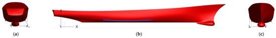
Figure 1.
Geometry of the DTMB model with bilge keels. (a): rear view; (b): profile; (c): front view.

Table 1.
Main particulars of the DTMB 5512 ship model.
The model was introduced as one of the three benchmark geometries in the Workshop on CFD in Ship Hydrodynamics that was held in Gothenburg in 2000 [17] along with two other geometries for conventional commercial ships; the first is the 300 K modern tanker called KVLCC, while the second is a 3600 TEU container model known as KCS. Both hulls were designed by the Korea Research Institute of Ships and Ocean Engineering (KRISO) formerly known as the Maritime and Ocean Engineering Research Institute (MOERI). The full scale DTMB ship does not exist; however, various geometrically similar models were built, tested and reported all over the world. Unlimited data base is available for the ship model in the public domain from experimental tests reported by very well recognized towing tank tests facilities such as the Istituto Nazionale per Studi Ed Esperienze di Architettura Navale (INSEAN) in Italy, Iowa Institute of Hydraulic Research (IIHR) which is now titled as IIHR–Hydroscience & Engineering in the United States of America, FORCE Technology of Denmark, Maritime Research Institute of Netherlands, (MARIN) and many others. Towing tank tests were performed and reported for different aspects in ship hydrodynamics, such as resistance, free-surface, local flow, propulsion, seakeeping, and maneuvering, all aimed at understanding the flow physics and providing a verification and validation reference for CFD applications. Table 2 provides a summary for the basic and most famous test cases performed on the DTMB models and reported by the previously listed institutes and research centers.
Table 2.
Benchmark test cases available in the public domain for the DTMB model reconstructed from [3,5,7,18,19,20].
From these tests, this study is an attempt by the authors to replicate the roll decay experiment performed by Irvine et al. in [3] using the CFD method, in order to validate the capability of the RANS modeling to predict the roll performance of the ship. This work is an extension of the previous attempt by the author that was introduced in [21] which was focusing on the same concept without taking into consideration the systematic verification of the CFD data, grid, and time-step effect on the numerical simulation, prediction, and validation of the viscous flow around the hull and particularly around the bilge keels and how it is affected by the turbulence model used. This is covered consistently in this study.
The analysis condition includes two levels of numerical simulations, the first intends to validate the numerical simulation against the experimental data, where the ship is sailing at a medium speed corresponding to a Froude number Fr = 0.138 where . This analysis condition covers different initial roll angle starting from 2.5 to 20 degrees with a step 2.5 degrees in every simulation. A special focus is applied for the 10 degrees condition, where the validation and verification of numerical result against experimental data takes place, following the same concept of case 3.6 from Gothenburg Workshop on CFD in ship hydrodynamics that was reported and summarized in the Workshop book [4]. The second level is aimed at investigating the effect of the ship speed on the roll damping of the ship. For this purpose, a set of five ship speeds is analyzed and reported for corresponding Froude numbers Fr = 0, 0.138, 0.20, 28, and 0.41 The viscous flow configuration around the ship hull and specifically around the bilge keel is also investigated and introduced.
3. The CFD Framework
3.1. Numerical Solver
All the numerical simulations performed in this study are carried out using the CFD viscous flow solver ISIS-CFD of the FINETM/Marine software which is available under the NUMECA umbrella. The solver implements the finite volume method to build the special discretization for the transport equation in order to solve the unsteady Reynolds-Averaged Navier–Stokes (RANS) equations. A face-based approach is used to construct the fluxes face by face, which makes the solver flexible for using any arbitrary shape control volume. This advantage makes it suitable to rely on the unstructured grids to easily discretize the complicated ship geometries and appendages. The temporal discretization is cell-centered based on a second order three-level scheme [22]. The velocity and pressure coupling in the governing equations is carried out using a Rhie and Chaw SIMPLE type algorithm, where the velocity field is obtained from the momentum equation, while the pressure is obtained from the mass constraint or continuity equation transformed into a pressure equation. Convection and diffusion terms in the governing equations are discretized using second-order upwind and central differencing scheme, respectively. Two-phase interface capturing technique is applied to predict the free-surface interface between air and water based on the Volume of Fluid (VOF) method, where the incompressible and non-miscible flow phases are modelled by introducing conservation equations of the volume fraction for each volume phase/fluid [22]. Various turbulence closures models are available within the code, from which, the blended Menter Shear Stress Transport K-ω SST model [23], and the Explicit Algebraic Reynolds Stress (EASM) model, which showed a promising success in predicting ship wake flow by code developer in [24] are chosen for this analysis, regarding to the reliable results previously obtained using both models by the author and in the marine applications in general.
3.2. Governing Equations
The time averaged continuity and momentum equations for the incompressible flow with external forces, can be written in tensor form, in the Cartesian coordinate system as
where is the relative averaged velocity vector of flow between the fluid and the control volume, is the Reynolds stresses, is the mean pressure and is the mean viscous stress tensor components for Newtonian fluid under the incompressible flow assumption, and it can be expressed as
3.3. Computational Domain and Boundary Conditions
The computational domain is configured as a rectangular prism whose dimension in (x-, y-, and z-) directions are imposed as (5.0 LWL, 4.0 LWL, and 2.5 LWL) distributed as follows: the upstream inflow boundary is located at 1.0 LWL from the Forward Perpendicular (F.P.); the outflow is located at 3.0 LWL downstream from the Aft Perpendicular (A.P.); the side boundaries are set at 2.0 LWL on both sides from the centerline of the ship; top and bottom boundaries are chosen to be at 1.0 LWL and 1.5 LWL above and underneath the undisturbed free-surface level, respectively. Figure 2 depicts the computational domain and the boundary conditions of the exterior boundaries.
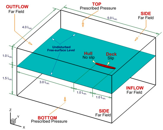
Figure 2.
Computational domain and boundary conditions.
No slip condition is applied for the ship hull, while the deck is set to slip condition, assuming that it remains in air during the simulation, where the viscous effect in the air compared to that in water can simply be ignored. Table 3 summarizes the initial conditions for the open boundaries and solid surfaces with respect to the simulation unknown quantities represented in: the three components of velocity U, V, and W; the pressure p; turbulent kinetic energy K; turbulent frequency dissipation ω; and finally, the mass fraction coefficient c in the VOF equation.
Table 3.
Boundary conditions for open boundaries and solid walls.
3.4. Discretization Grids
The discretization grid is generated using the HEXPRESSTM module included in the FINETM/Marine package which represents an automatic unstructured hexahedral grid generator. The grid generation process is initiated based on the validation case parameters; i.e., the ship velocity is corresponding to Fr = 0.138. This is considered acceptable from the numerical grid generation point of view, since the other test cases are subjected to a higher speed, which means that the refinement parameters for free-surface and hull vicinity will be implicitly sufficient. The grid is generated at the upright condition corresponding to an initial inclination angle equals zero. This provides better control for the symmetry of the grid on both sides; however, since the simulation will include significant inclination angles up to 20 degrees, it is difficult to control the stability of the grid deformation without having any grid issues. One of the common techniques followed in this case is to use an overset or sliding grid technique; nevertheless, it is rather more complicated and not straightforward; besides, they usually require larger memory. In order to avoid this problem, an isotropic refinement box was applied (as shown in Figure 3b,c) containing the entire ship and extended at 0.1 LWL from the A.P. in x-direction behind the ship, while the forward face is set slightly ahead the F.P., the box side faces are positioned at 0.25 LWL in y-direction and finally, the box height is extended 0.075 LWL and 0.065 LWL in z-direction underneath and above the ship base line, respectively. An extra refinement box is applied in the vicinity of the bilge keel aimed at capturing more flow details in that zone (as shown in Figure 3c,d). Finally, the free-surface is refined using a Kelvin-pattern-like refinement section having an opening angle of 60 degrees, equally distributed on both sides with respect to the ship centerline, and longitudinally extended about 2.0 LWL behind the hull (as shown in Figure 3e). The longitudinal and horizontal refinement imposed on the Kelvin pattern section is imposed to provide 60 grid cells per wave length in x- and y-directions, i.e., Δx = Δy = 2πFr2 LWL/60; while in z-direction, the thickness of the refinement zone is chosen to cover the stagnation wave amplitude defined by ζmax = 0.5 U2/g, The cell size in z-direction for the free-surface refinement sector is chosen as Δz = 0.001 LWL. The fine grid details are plotted in Figure 3 showing the entire grid with longitudinal, lateral and horizontal sections to highlight the box refinement around the hull and the free-surface refinement, respectively.
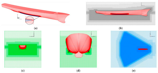
Figure 3.
The finest discretization grid. (a): entire 3D hull grid; (b): longitudinal section showing the refinement zone; (c,d): transversal section showing the refinement boxes in the vicinity of hull and bilge keel, respectively; (e): top view showing the free-surface refinement zone.
In the scope of performing a verification and validation study, a special focus on the numerical simulation errors is considered for both grid and time step. Four grids are generated for this purpose, where the first grid is globally refined systematically in order to obtain a geometrically similar grid configuration to apply the Richardson Extrapolation method. Despite the fact that it is rather difficult to maintain the grid similarity in the unstructured grids, a systematic methodology previously applied by the author in [25] following the same concept proposed in [26] can maintain the grid similarity, especially before the viscous layer insertion. The concept is based on changing two parameters involving the initial grid cell size and the refinement diffusion depth. This resulted in a set of four systematically varied grids with an initially targeted grid refinement ratio of rG = 1.5, that actually resulted in an average grid refinement ratio within rG ≈ 1.457. The summary of the generated grids is tabulated in Table 4, where M1 refers to the finest mesh and M4 refers to the coarsest.
Table 4.
Computational grids for the grid convergence study.
3.5. Simulation Strategy
The simulation is performed in two levels considerably similar to the strategy applied in the experiment; in the first simulation, the ship is towed ahead with the corresponding forward speed and imposed roll angle in order to change the roll angle from zero degree to the desired angle within an acceleration period of 8 s, computed based on the equation Tacc = 2.0 LWL/U. This simulation is performed until the flow around the hull is stabilized; 40 s were selected to insure a sufficient stabilization period. The time step in this case is selected similar to the general resistance tests with respect to the ITTC recommended procedures [12,27] such that Δt = 0.005 LWL/U which resulted in Δt = 0.02 s and only 8 nonlinear iterations were considered sufficient to maintain the residuals within an acceptable level. The second simulation continues from where the first simulation ends, towed a head with the ship free to roll in order to record the roll response of the ship. The number of nonlinear iterations is increased to 12 in this case and the time step is reduced to Δt = 0.005 s, which is 3 times less than the ITTC recommendations for roll decay simulations. The simulation is performed for at least six full roll periods to provide sufficient number points for comparison against EFD data. All the computations are performed on a High Performance Computing (HPC) machine with available 120 cores at 2.5 up to 3.3 GHz, with the number of cores is sometimes divided according to the grid density (e.g., 48/72 cores for coarser grids and the total 120 cores for the finest grids). The total computation time for first level simulation is within 13–38 physical hours, while for the second level freed roll simulation, the total computation time is within 22–73 h, which are definitely influenced by the grid resolution, time step and number of cores used in the simulation.
4. Results and Discussion
4.1. Results Validation
In order to investigate the accuracy of the applied method in predicting the roll decay behavior of the DTMB ship, a direct comparison between the CFD results and EFD data is performed at different roll angle for the medium speed range condition; i.e., Fr = 0.138. The comparison is brought to attention in Figure 4 for initial roll angles from = 2.5° to 20°, step 2.5°. The comparison shows that the computed results resembles accurately with the measured data, except for a slight discrepancy in the peak points of roll motion response for the first, second and sometimes the third roll period, otherwise the rest are within a proper coherence. A slight over-prediction was also recorded for the computed roll period compared to the EFD data, where the computed roll period TCFD = 1.572 s while the one reported by Irvine et al. [3] in the test was TEFD = 1.54 s. The percentage error for the computed CFD roll period is within 2.1%, which is assumed to be within an acceptable range. As for the amplitudes of the roll motion, the error range was measured within 1.06% and 24.28% for the minimum and maximum deviated values, respectively. The simulation values tend to depart from the measured ones, especially for the second period as the initial roll angle increases; this might be related to one of two reasons: the first might be as a consequence for the instability of the turbulence model, as the accuracy of the turbulence model may encounter stability drawbacks when a severe flow separation occurs; or the other reason might be related to the grid consistency after deformation for the large angles of motion, which might cause some numerical issues and consequently results in this deviation. Best resemblance was recorded for initial roll angles = 2.5 and 5°, while the highest error was recorded for the peaks of the second and third periods for the initial roll angles of = 15 and 20°.
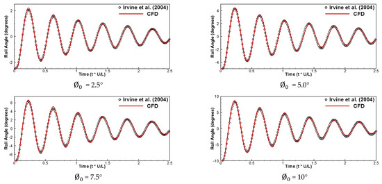
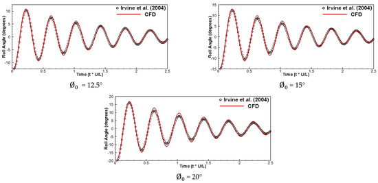
Figure 4.
Roll angle simulation history for various initial roll angles.
4.2. Validation with the Fitted Decay Curve
The results from the main simulation case that is assigned for validation in this study which is corresponding to the initial roll angle = 10° and Fr = 0.138 for the finest grid are used to plot the decay curve based on the mean value of the decay response, which can be computed as the average value between two consecutive roll peaks such that: and the decrement of the roll angle computed based on the equation according to the ITTC recommended procedures [12]. The fitted curve should be represented as a third-degree polynomial whose constants a, b, and c are representing the extinction coefficients according to the equation
The numerically computed results for the decay extinction curve obtained from the peaks of the roll motion are presented in Table 5 compared to the EFD data, while the diagram is plotted in Figure 5. The results shows that the maximum absolute computed error for the obtained CFD results is about 7.519%, while the minimum is 1.06% and finally, the average error is about 4.245%, which may be considered within a reasonable range.
Table 5.
Results for the motion amplitudes and decay fitting curves parameters.
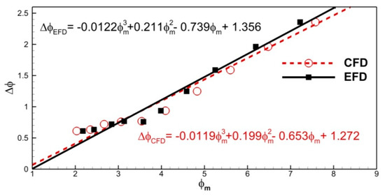
Figure 5.
CFD vs. EFD fitted decay curves computed based on the roll amplitudes.
4.3. Verification and Validation of the Numerical Errors
A systematic verification and validation procedures are performed in order to assess the numerical errors through a grid and time step convergence studies, based on the generalized Richardson Extrapolation (RE) method that is explained in details in [28,29]. First, the verification study is applied to assess the numerical uncertainty USN, which can be expressed as
where represents the iterative uncertainties, represents for the grid uncertainties, stands for the time step uncertainty and finally, stands for any other parameter. The iterative uncertainties in this study were ignored as they were found to be very small in comparison to the grid and the time step uncertainties. The verification procedures start with the convergence study based on the convergence ratio that can be estimated based on the equation
According to the ITTC guidelines presented in [28] Equation (6) imposes three different conditions such that
- Monotonic convergence:;
- Oscillatory convergence: , ;
- Divergence:.
If a monotonic convergence is achieved, the RE error can be estimated based on the refinement ratio and the order of accuracy according to Equation (7)
and the uncertainty can be estimated by imposing the correction method or the factor of safety as proposed in the ITCC [28]. However, in roll decay, the convergence test requires the uncertainty of a point variable where the evaluation of , and can propose a problem where the solution changes can tend to zero. For this reason, the profile average value can be used instead and it can be estimated as
For the second condition, if an oscillatory convergence is achieved, the uncertainty is estimated using the lower and upper values of oscillation and , respectively, such that
and finally, if the monotonic divergence condition is achieved, this means that the errors and uncertainties cannot be estimated.
On the other hand, the validation is accomplished through comparing the estimated error E with the validation uncertainties UV based on the data uncertainty UD, according to the equation
When |E| is within range, solutions are validated at the interval; otherwise, the results might be validated at another required validation level ; else, the results are not validated.
The computed parameters for the grid convergence study are tabulated in Table 6 for the four grids, where M1 indicates the finest grid, while M4 specifies the coarsest. The results have a descending behavior where the coarsest grid seems to over predict the roll amplitude almost within the six periods of the simulation time. In addition, a slight phase shift can be noticed between the finer and coarser grids. On the other hand, as the grid density increases, the results resemble closer to the EFD data, as expected, and the finest two grids show almost similar values for the roll amplitudes. Globally, a monotonic convergence is obtained for the grid convergence study where the grid convergence ratio = 0.517. However, locally when focusing on the fourth and fifth amplitudes, the value was alternating between M2 and M1 showing a local oscillatory convergence.
Table 6.
Results for grid convergence study.
As for the time convergence study, the effect of changing the time step was not significant. This gives a proper indication about the choice of time step; since the criteria proposed by the ITTC states that the proper time step for CFD simulations should be within 100 time steps per roll period, while the initial time step applied in this study provides 325 time steps per roll period. This value was divided by two in every level to provide a finer time step for the next simulation. Taking into consideration the fact that the difference between the simulations was highly insignificant, and following the same experience from other researches, for example [14,30], in which they concluded that the time step had a minor effect on the computed results; only the first period was tested because the simulation physical time was increasing dramatically. The time step convergence parameters are listed in Table 7, while the time history for grid and time step convergence is plotted in Figure 6.
Table 7.
Results for time-step convergence study.
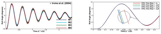
Figure 6.
Roll decay curves for the grid convergence test (left) and the time step convergence test (right).
The validation results are presented in Table 8 showing that the average computed error should be within 4.063%, this means that the results are not validated to the level as the average error for the finest grid is within 4.245%. Nevertheless, the results are still within an acceptable range of accuracy, especially for the finest grids M1 and M2 as the error range lies beneath 5% which could be considered reasonable.
Table 8.
Results for validation study.
4.4. Local Flow Analysis
Analysis of local flow of the ship in different simulation conditions can give a proper understanding of the flow configuration around the hull especially for the present study, where the flow is expected to have a strong interaction with the hull and specifically with the bilge keels. As the turbulence model can influence the well prediction of the velocity contours and flow wake in the RANS solvers, two turbulence models were investigated, Menter’s K-ω SST and Explicit Algebraic Stress Model (EASM) to study their accuracy and their capability to predict the expected flow separation and vortex shedding. In ship hydrodynamic field, both models have proven to be very successful for the wake and flow separation prediction for various types of ships; however, EASM requires longer simulation time as the time step should be adapted accordingly to enhance the convergence of the model, as it was proposed by the ITTC recommended procedures [12].
In order to investigate the accuracy of our simulation in predicting the local flow, the computed and measured [3] data for the transversal section positioned at x = 0.675 Lpp from the forward perpendicular are depicted in Figure 7 for two phases from the second roll cycle: the first is when the ship is reaching the trough of the cycle, while the second is when the ship is reaching the zero position heading back to the crest of the third cycle. As previously explained, the validation process is always presented here for the condition when the initial roll angle is = 10° and the Fr = 0.138. From the given comparison; it can be observed that the computed velocity contours have a proper agreement with the measured data, though it can be noticed that it is slightly under predicted and the computed streamwise velocity contours seems to be more contracted towards the hull. The agreement between the contours computed based on the EASM model resembles better than the one obtained using K-ω SST model, yet both are having a satisfying level of accuracy.
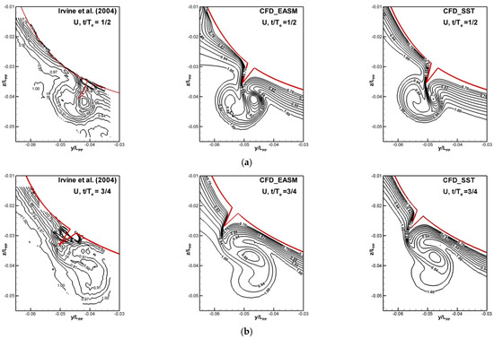
Figure 7.
Axial velocity contours at section x/Lpp = 0.675 measured at the second period of roll at: (a) t/T = 1/2; (b): t/T = 3/4.
In the scope of studying the flow configuration around the hull, a proper understanding of the mechanism of the vortices generated during the roll decay process is necessary. For this reason, Figure 8a depicts the iso-surface second invariant Q* = 25 colored by the non-dimensional helicity for the hull bottom view obtained using the EASM turbulence model when the ship is at the four quarter phases of the second roll period i.e., t/T = 0, 0.25, 0.50, and 0.75. In addition, Figure 8b,c are showing the side view of the generated vortices at t/T = 0 from starboard and port sides, respectively. The generated vortical structures are quite similar to the ones predicted in the study reported in [13], except the fact that both turbulence models could not capture the full vortical structures till the ship stern, it seems like it dissipated directly after the amidships. Near the ship bow, the mechanism consists of two layers of vortical tubes that are resulting after the flow shedding from the sonar dome named as Sonar Dome Vortices (SDV) and the ones generated at the intersection of the keel with the sonar dome named the Fore-Body Keel Vortices (FBKV). The SDV dissipates faster slightly after the first third of the ship length, while the FBKV continues downstream. Unlike the straight formation expected in the classic resistance test, the vortical structure of the FBKV is having a sinusoidal fluctuating behavior horizontally and vertically, apparently due to the ship rolling effect as Figure 8 bears out. Heading downstream, the Bilge Keel Vortices (BKV) are generated at the forward tip of the bilge keel and continues downstream.
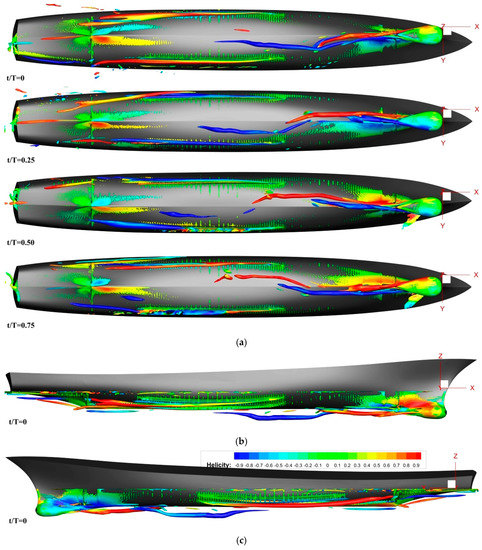
Figure 8.
The iso-surface second invariant Q* = 25 colored by the non-dimensional helicity at the peak of the second period of roll t/T = 0, 0.25, 0.5 & 0.75 showing: (a) bottom, (b) starboard side and (c) port side views, respectively for t/T = 0.
The BKV are split in two counter rotating vortices on each side of the bilge keel (suction and pressure sides), or it can be said beneath and above the bilge keel when the ship is at the peak or the trough of the roll motion. The intensity changes and the interaction between these two vortices with respect to the ship roll motion can be observed (see Figure 9).
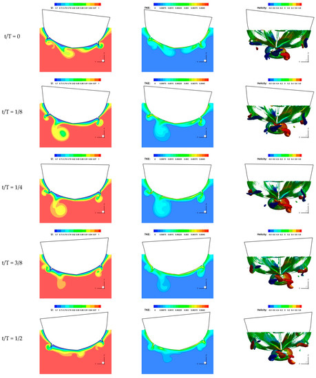
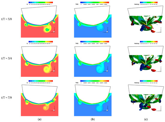
Figure 9.
Local flow characteristics at section x/Lpp = 0.675 at 8 instances from the second period of roll. (a): streamwise velocity contours U; (b): turbulent kinetic energy TKE; (c): Second invariant Q* = 25 colored by non-dimensional helicity.
If we combine those vortical structures along with the streamwise velocity and the Turbulent Kinetic Energy (TKE) contours as Figure 9 bears out, the entire picture for the flow evolution in the vicinity of the hull and bilge keels during the roll decay process can be comprehended.
The streamwise velocity contours suffers an obvious deformation as the flow is converted from the high momentum zone to the boundary layer where both vortical structures are apparently combined, rotating inward and positioned underneath the bilge keel when the ship is reaching the peak of the roll motion (t/T = 0 and t/T = 1/8). When the ship returns back to the 0 position, both BKV can be visualized as they are positioned on both sides of the keel, and the boundary layer appear to be evenly distributed on the both sides of the ship. Mirror-like effect with less intensity as the roll angle is decreased by the damping effect happens as the ship heads to the trough of the roll motion, where the starboard side vortices are almost combined this time at the trough of the roll motion and moved underneath the bilge keel (t/T = 3/8 and t/T = 1/2). The same process continues as the ship rolls until the full decay is achieved. The consumed energy during this cyclic process of vortex shedding contributes in the increment in ship resistance.
4.5. Free-Surface Analysis
The free-surface topology for the medium speed condition is plotted in Figure 10 for the four quarter phases of the second period of roll motion at Fr = 0.28 and initial roll angle = 10°. It can be observed that the free-surface is affected by the viscous and pressure effect on the hull resulted from the roll motion of the ship. Though for this ship speed the free-surface seems to be consistent, the influence of the ship motion can be observed in the vicinity of the hull, were the viscous effect at the hull skin resulted from the no-slip condition induces a vertical velocity that creates a crest or trough based on the ship heeling angle. This adds or subtract from the generated Kelvin waves. Similarly, the pressure effect pushes the flow laterally as the ship rolls causing the crest or the trough of the of the Kelvin waves to propagate upstream, resulting in a slight distortion in the generated waves as it can be observed in the vicinity of the hull, especially after the forward shoulders. This effect is less observed as the ship speed increases, as it will be observed in the following section at Fr = 0.41 case.
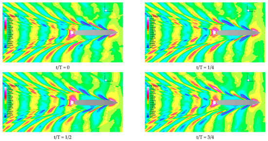
Figure 10.
Free-surface at the four quarters of the second roll period for = 10 and the Fr = 0.28.
4.6. Ship Speed Effect
In order to investigate the effect of ship speed on the roll damping process, five ship speeds were tested for the initial roll angle condition = 10° having Fr = 0.0, 0.138, 0.2, 0.28, and 0.41, respectively. It is worth mentioning that for the zero speed case an approximation was applied, since the program does not accept a stationary ship. For this purpose, a very small speed was imposed for the flow 1 × 10⁻³ which is corresponding to an order of magnitude less Froude number meaning a very close value to zero. The results for the five ship speeds are plotted for a qualitatively comparison purpose in Figure 11. The comparison reveals that the roll damping increases as the ship speed increases which tends to diminish the motion amplitudes after the fourth cycle for the Fr = 0.41. This observation has also been concluded in the tank tests performed and reported in [3,7].
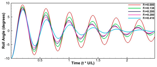
Figure 11.
Roll decay curves varying based on the ship velocity for Fr = 0.0, 0.138, 0.20, 0.28, and 0.41, respectively.
From another perspective, the effect of the velocity on the free-surface is brought to attention in Figure 12 that represents the absolute wave elevation for all five simulation cases at the end of the sixth period of oscillation. At the zero speed condition, the wave elevation is very small and it is influenced only by the roll motion of the hull. For both cases when Fr = 0.138 and 0.20, the aforementioned viscous and pressure effects from the hull are present, where a generated Kelvin pattern is not very well developed due to the lower speed of the ship, a high interaction between the hull and surrounding waves can be visualized causing a change in the generated Kelvin wave pattern. The same observation for the low speed in other researches also persists here, as it can be concluded that only 60 cells/wave length lacks a proper predicting for the free-surface development. This may require increasing this value for better results. A slight effect in the Fr = 0.41 case can also be observed, showing that as the speed increases, the wave-hull interaction decreases.
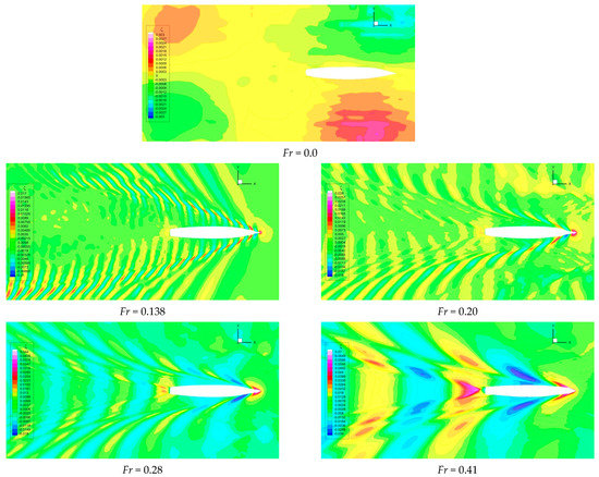
Figure 12.
Free-surface topology at the end of the 6th-period of roll for different ship speeds.
5. Conclusions
The CFD simulation for the free roll decay of the DTMB 5512 surface combatant ship model sailing in calm water and appended with bilge keels was performed based on unsteady RANS where the closure to turbulence was achieved using the K-ω SST and the EASM models. The simulation is executed for different initial roll angles and for various ship speeds in order to investigate their influence on the roll decay of the ship. Standard deforming unstructured grid approach with a special refinement in the vicinity of the hull and close to the interface was implemented to count for the expected large ship motion rather than using overset or sliding grid, where they have some relative drawbacks compared to the standard grids represented in their complexity and the large required memory for simulation. The initial validation of the roll decay at different initial roll angles was qualitatively and quantitatively investigated in comparison with the EFD data showing that the resemblance between the CFD and EFD was satisfying, especially for the computed roll period which was estimated with less than 2% error; on the other hand, the discrepancies in roll amplitudes were significant for the second and sometimes the third roll period with an error up to 24.28%. The amplitude deviation was increasing as the initial roll angle increases.
Verification and validation (V&V) study based on the Richardson Extrapolation method was performed based on grid and time step convergence study with four geometrically similar grids and four time steps, respectively. The V&V study showed a global monotonic convergence for the predicted roll amplitude and occasionally local oscillatory convergence as the finest grids results were very close in values. Validation was not achieved at the validation uncertainty level where the average estimated error for computed data was 4.245% and = 3.378%; nevertheless, the average error was considered acceptable especially for the finest grids.
Since the roll decay is dominated by the viscous effect, a special focus on the flow in the vicinity of the hull and specifically at the bilge keel was presented by means of velocity field, TKE and vortex formation showing the interaction between the hull and surrounding flow during roll motion, which tends to impose an oscillation in the vortical tubes dissipated from the sonar dome and the keel vortices, both horizontally and vertically. On the other hand, the vortex formation around the bilge keels and its development was also represented showing the interaction between the bilge keel and the surrounding flow during the roll second period.
Roll decay influence on the free-surface was also illustrated showing the effect of the body motion on the Kelvin wave pattern during the simulation, which resulted in a slightly deformed Kelvin wave pattern due to the viscous and pressure effects imposed by the roll damping process. In addition, the effect of the speed on the free surface, as well as on the roll damping, which showed to be compatible with the same conclusions for the similar tank tests. For the low speed cases, it was concluded that only 60 cells/wave length is not adequate to predict the full development of the free-surface at that speed.
Overall, comparing the main objective of this study with the outcomes, it can be said that the implemented approach was successful in predicting the roll decay of the ship. Some discrepancies exist for different parameters, yet they are not very significant and they could be considered more than satisfying for initial design and for optimization purposes. Though the simulation time was relatively high, yet the flexibility of the simulation method makes it feasible compared to experimental method. Obviously, the integration between CFD and EFD is the key for improving the ship design process and for solving more complicated ship hydrodynamic problems.
Despite the fact that the turbulence model performed well, as it was illustrated in this study, more details in the flow could be captured using DES or LES models and can help in providing more understanding for the flow mechanism around the bilge keels. This can be a base for further investigation.
Author Contributions
Conceptualization, A.B.; methodology, A.B.; validation, A.B., formal analysis, A.B.; investigation, A.B.; data curation, A.B.; writing—original draft preparation, A.B.; writing—review and editing, A.B.; visualization, F.P.; supervision, F.P.; project administration, F.P. All authors have read and agreed to the published version of the manuscript.
Funding
This research received no external funding.
Institutional Review Board Statement
Not applicable.
Informed Consent Statement
Not applicable.
Data Availability Statement
Data sharing is not applicable to this article.
Acknowledgments
This work was carried out in the framework of the research project DREAM (Dynamics of the REsources and technological Advance in harvesting Marine renewable energy), supported by the Romanian Executive Agency for Higher Education, Research, Development and Innovation Funding—UEFISCDI, grant number PN-III-P4-ID-PCE-2020-0008.
Conflicts of Interest
The authors declare no conflict of interest.
References
- Falzarano, J.; Somayajula, A.; Seah, R. An overview of the prediction methods for roll damping of ships. Ocean Sys. Eng. 2015, 5, 55–76. [Google Scholar] [CrossRef]
- Bassler, C.C.; Reed, A.M. An analysis of the bilge keel roll damping component model. In Proceedings of the 10th International Conference on Stability of Ships and Ocean Vehicles (STAB2009), St. Petersburg, Russia, 22–26 June 2009; Degtyarev, A.B., Ed.; Glasgow, Scotland, UK, 2009; pp. 369–386. [Google Scholar]
- Irvine, M.; Longo, J.; Stern, F. Towing tank tests for surface combatant for free roll decay and coupled pitch and heave motions. In Proceedings of the 25th Symposium on Naval Hydrodynamics, St Johns, NL, Canada, 8–13 August 2004; National Academy of Sciences, the National Academies Press: Washington, DC, USA, 2005. [Google Scholar]
- Larsson, L.; Stern, F.; Visonneau, M. (Eds.) Numerical Ship Hydrodynamics, an Assessment of the Gothenburg 2010 Workshop; Springer: Dordrecht, The Netherlands, 2013; pp. 190–196. [Google Scholar]
- Aloisio, G.; Di Felice, F. PIV analysis around the bilge keel of a ship model in a free roll decay. In Proceedings of the XIV Congresso Nazionale A. I. VE. LA., Rome, Italy, 6–7 November 2006. [Google Scholar]
- Irkal, M.A.; Nallayarasu, S.; Bhattacharyya, S. CFD approach to roll damping of ship with bilge keel with experimental validation. Appl. Ocean Res. 2016, 55, 1–17. [Google Scholar] [CrossRef]
- Atsavapranee, P.; Carneal, J.B.; Grant, D.; Percival, A.S. Experimental investigation of viscous roll damping on the DTMB model 5617 hull form. In Proceedings of the ASME 26th International Conference on Offshore Mechanics and Arctic Engineering, San Diego, CA, USA, 10–15 June 2007. OMAE2007-29324. [Google Scholar]
- Begovic, E.; Day, A.H.; Incecik, A.; Mancini, S.; Pizzirusso, D. Roll damping assessment of intact and damaged ship by CFD and EFD methods. In Proceedings of the 12th International Conference on the Stability of Ships and Ocean Vehicles, Glasgow, UK, 13–19 June 2015; pp. 14–19. [Google Scholar]
- Piehl, H.P. Ship Roll Damping Analysis. Ph.D. Thesis, Faculty of Engineering, Maschinenbau und Verfahrenstechnik, Institute of Ship Technology, The University of Duisburg-Essen (UDE), Duisburg, Germany, 22 April 2016. [Google Scholar]
- Ikeda, Y.; Himeno, Y.; Tanaka, N. A Prediction Method for Ship Roll Damping; Department of Naval Architecture, University of Osaka Prefecture: Osaka, Japan, 1978. [Google Scholar]
- Kawahara, Y.; Maekawa, K.; Ikeda, Y. Characteristics of roll damping of various ship types and a simple prediction formula of roll damping on the basis of Ikeda’s method. In Proceedings of the 4th Asia-Pacific Workshop on Marine Hydrodynamics, Taipei, Taiwan; 2008; pp. 79–86. [Google Scholar]
- ITTC. Recommended Procedures and Guidelines: Numerical Estimation of Roll Damping; 7.5-02 -07-04.5, 2011, Rev. 00; ITTC: Rio de Janeiro, Brazil, 2011; pp. 1–32. [Google Scholar]
- Wilson, R.V.; Carrica, P.M.; Stern, F. Unsteady RANS method for ship motions with application to roll for a surface combatant. Comput. Fluids 2006, 35, 501–524. [Google Scholar] [CrossRef]
- Gokce, M.K.; Kinaci, O.K. Numerical simulations of free roll decay of DTMB 5415. Ocean Eng. 2017, 159, 539–551. [Google Scholar] [CrossRef]
- Begovic, E.; Mancini, S.; Day, A.H.; Incecik, A. Applicability of CFD Methods for Roll Damping Determination of Intact and Damaged Ship. In High Performance Scientific Computing Using Distributed Infrastructures; Andronico, G., Bellotti, R., De Nardo, G., Lacetti, G., Maggi, G., Merola, L., Russo, G., Silvestris, L., Tassi, E., Eds.; Toh Tuck Link: Singapore, 2015; Chapter 29; pp. 343–359. [Google Scholar]
- Gao, Q.; Vassalos, D. Numerical study of the roll decay of intact and damaged ships. In Proceedings of the 12th International Ship Stability Workshop, Session 7 Stability of Damaged Ships—Numerical Simulation of Progressive Flooding and Capsize, Washington, DC, USA, 12–15 June 2011. [Google Scholar]
- Larsson, L.; Stern, F.; Bertram, V. (Eds.) A Workshop on Numerical Ship Hydrodynamics, Proceedings Gothenburg 2000; Chalmers University of Technology: Gothenburg, Sweden, 2000. [Google Scholar]
- ITTC. Recommended Procedures and Guidelines: Benchmark Databases for CFD Validation for Resistance and Propulsion; 7.5-03 -02-02, 2017, Rev. 01; ITTC: Wuxi, China, 2017; pp. 1–9. [Google Scholar]
- Irvine, M.; Longo, J.; Stern, F. Pitch and heave tests and uncertainty assessment for a surface combatant in regular head waves. J. Ship Res. 2008, 52, 146–163. [Google Scholar] [CrossRef]
- Workshop on Verification and Validation of Ship Manoeuvring Simulation Methods, SIMMAN2014. Available online: https://simman2014.dk/ship-data/us-navy-combatant/overview-of-tests-us-navy-combatant/ (accessed on 14 April 2021).
- Bekhit, A.S.; Lungu, A. Numerical free roll decay prediction for the DTMB hull. In AIP Conference Proceedings, Proceedings of the 16th International Conference on Numerical Analysis and Applied Mathematics, ICNAAM 2018, Rhodes, Greece, 13–18 September 2019; American Institute of Physics: Melville, NY, USA, 2019; Volume 2216, p. 450050. [Google Scholar]
- Queutey, P.; Visnonneau, M. An interface capturing method for free-surface hydrodynamic flows. Comput. Fluids 2007, 36, 1481–1510. [Google Scholar] [CrossRef]
- Menter, F.R. Zonal two equation kappa-omega turbulence models for aerodynamic flows. In Proceedings of the 24th AIAA Fluid Dynamics Conference, Orlando, FL, USA, 6–9 July 1993. [Google Scholar]
- Guilmineau, E.; Deng, G.B.; Leroyer, A.; Queutey, P.; Visonneau, M.; Wackers, J. Influence of the turbulence closures for the wake prediction of a marine propeller. In Proceedings of the 4th International Symposium on Marine Propellers (SMP’15), Austin, TX, USA, 31 May–4 June 2015. [Google Scholar]
- Bekhit, A.; Obreja, D. Numerical and experimental investigation on the free-surface flow and total resistance of the DTMB surface combatant. In Proceedings of the 8th International Conference on Modern Technology in Industrial Engineering, MODTECH 2020, Romania, Online Edition. 23–27 June 2020; Volume 916, p. 012008. [Google Scholar]
- Crepier, P. Ship resistance prediction: Verification and validation exercise on unstructured grids. In Proceedings of the 7th International Conference on Computational Methods in Marine Engineering, Nantes, France, 15–17 May 2017; Visonneau, M., Queutey, P., Le Touzé, D., Eds.; CIMNE: Barcelona, Spain, 2017; pp. 365–376. [Google Scholar]
- ITTC. Recommended Procedures and Guidelines: Practical Guidelines for Ship CFD Applications; 7.5-03 02-03, 2011, Rev. 01; ITTC: Rio de Janeiro, Brazil, 2011; pp. 1–18. [Google Scholar]
- ITTC. Recommended Procedures and Guidelines, Uncertainty Analysis in CFD Verification and Validation Methodology and Procedures; 2017, Rev. 03; ITTC: Wuxi, China, 2017; pp. 1–12. [Google Scholar]
- Stern, F.; Wilson, R.V.; Coleman, H.W.; Paterson, E.G. Comprehensive approach to verification and validation of CFD simulations—Part 1: Methodology and procedures. Fluids Eng. 2001, 123, 793–802. [Google Scholar] [CrossRef]
- Mancini, S.; Begovic, E.; Dayb, A.H.; Incecik, A. Verification and validation of numerical modelling of DTMB 5415 roll decay. Ocean Eng. 2018, 162, 209–223. [Google Scholar] [CrossRef]
Publisher’s Note: MDPI stays neutral with regard to jurisdictional claims in published maps and institutional affiliations. |
© 2021 by the authors. Licensee MDPI, Basel, Switzerland. This article is an open access article distributed under the terms and conditions of the Creative Commons Attribution (CC BY) license (https://creativecommons.org/licenses/by/4.0/).