Article

Operational Analysis of Container Ships by Using Maritime Big Data

1
School of Naval Architecture and Ocean Engineering, University of Ulsan, Ulsan 44610, Korea
2
Research Institute of Marine Systems Engineering, Seoul National University, Seoul 08826, Korea
3
Department of Naval Architecture and Ocean Engineering, Seoul National University, Seoul 08826, Korea
4
Interdisciplinary Program in Offshore Plant Engineering, Seoul National University, Seoul 08826, Korea
5
ICT Solution Team, Digital Technology Center, Korean Register, Busan 46762, Korea
6
Digital Technology Center, Korean Register, Busan 46762, Korea
*
Author to whom correspondence should be addressed.
J. Mar. Sci. Eng. 2021, 9(4), 438; https://doi.org/10.3390/jmse9040438
Submission received: 19 February 2021 / Revised: 14 April 2021 / Accepted: 15 April 2021 / Published: 18 April 2021
(This article belongs to the Special Issue Simulation Based Maritime Design)

Abstract

:
The shipping company or the operator determines the mode of operation of a ship. In the case of container ships, there may be various operating patterns employed to arrive at the destination within the stipulated time. In addition, depending on the influence of the ocean’s environmental conditions, the speed and the route can be changed. As the ship’s fuel oil consumption is closely related to its operational pattern, it is possible to identify the most economical operations by analyzing the operational patterns of the ships. The operational records of each shipping company are not usually disclosed, so it is necessary to estimate the operational characteristics from publicly available data such as the automatic identification system (AIS) data and ocean environment data. In this study, we developed a visualization program to analyze the AIS data and ocean environmental conditions together and propose two categories of applications for the operational analysis of container ships using maritime big data. The first category applications are the past operation analysis by tracking previous trajectories, and the second category applications are the speed pattern analysis by shipping companies and shipyards under harsh environmental conditions. Thus, the operational characteristics of container ships were evaluated using maritime big data.

1. Introduction

In global supply chains, maritime transport has the largest volume of trade. Bell and Meng [1] emphasized that the maritime transport industry is facing major challenges concerning freight rates, fuel prices, environmental sustainability, etc. These challenges need to be addressed to ensure greater efficiency. The importance of sustainable development in liner shipping management is also emphasized by Vejvar et al. [2]. The authors identified four major research domains in liner shipping management. One of them is shipping performance. The fuel oil consumption is a factor in evaluating shipping performance. Le et al. [3] proposed voyage-based statistical fuel consumption models, and Kim et al. [4] suggested a method to estimate the fuel oil consumption using the AIS data and ocean environmental data. Additionally, container shipping influences supply chain integration all over the world [5]; therefore, it is important to analyze container ships’ operations for sustainable development.
In this study, we present a method to streamline container ships’ operations by analyzing maritime big data, such as automatic identification system (AIS) data and ocean environment data. Big data technologies have become very popular in many industries of late. We applied these technologies to analyze the big size of data. As a result, it was possible to obtain the operational characteristics of container ships, such as average speed, waiting time at ports, and the efficiency of voyage compared to other ships. As the characteristics can affect the operational cost directly, it can be used to evaluate the efficiency of the operation. Therefore, the operational characteristics leveraged from maritime big data can improve the operations of container ships.
The operational characteristics of container ships are different for each shipping company or operator. Some operators control the speed of the ship to coincide with the appointed arrival time at a port. On the other hand, other operators run the ships fast and prefer to wait near the port to enter. The operational characteristics are closely related to fuel oil consumption, thus affecting the operational expenditure. Shipping companies can reduce their cost by analyzing and optimizing the operations. Furthermore, they can compare their shipping efficiency to that of their competitors’ by comparing operational characteristics. Generally, shipping companies do not disclose their operational profile, making it difficult to compare the operational efficiency of different companies. The fuel oil consumption is the most important factor to estimate the efficiency of the ship. However, it is difficult to calculate the fuel oil consumption because gathering that information is expensive [3]. Furthermore, this information is not published in general, even if it is gathered. Therefore, it is necessary to obtain the operational characteristics from publicly available data such as the AIS data [6,7]. In addition, the ocean environmental conditions, for instance, wind, wave, current, significant wave height, etc., can affect the operations. The size of the AIS and ocean environment data is very large, making it necessary to use big data technologies. Nowadays, big data technology is developing rapidly, and a lot of valuable information is obtained by big data analysis. In this study, we combined the two different big data to analyze the operations of container ships. We present the operational analysis methodology of container ships by analyzing the maritime big data using big data technologies. Two categories of the applications are proposed for the operational analysis of container ships; one is the past operation analysis by tracking previous trajectories, and the second is the speed pattern analysis by shipping companies and shipbuilders. For a better understanding of the analysis results, we developed a visualization program for the AIS data and ocean environment data.
The purpose of this study was to present some applications that can be obtained from the big data analysis. This study may not include a novel algorithm to obtain the result but can be considered a practical study to introduce the applications using the public operational data.
The remainder of the paper is structured as follows. The related work is described in Section 2. Section 3 presents the maritime big data used for the operational analysis of container ships, and the big data framework to process the big data. In addition, the developed visualization program for the analysis was also introduced in Section 3. The applications of the maritime big data analysis are presented along with the discussion in Section 4, and the paper is concluded in Section 5.

2. Related Work

Some earlier studies have presented applications using the AIS data. Yang et al. [8] conducted a review of the AIS data applications. The authors reviewed many AIS data applications, from simple data collections to vessel performance monitoring. Related to this, one of the applications was proposed by Jia et al. [9]. The seaborn transport pattern maps could be generated using the AIS data. The author also proposed the estimation method of vessel payloads in bulk shipping using the AIS data [10]. Perera et al. [11] proposed a decision-making system for ship collision avoidance, and the AIS data were used to obtain the navigational information. Wen et al. [12] suggested a model that evaluated the maritime traffic flow complexity and proposed that marine traffic could be measured using the AIS data that are used in most ports to collect information regarding the position, course, and speed of each ship. A method for restoring the trajectory of inland waterway ships using the AIS data was proposed by Sang et al. [13]. The authors proposed a method of cleansing the AIS data, and a trajectory restoring method using the line, curve, and arc. To predict the destination and arrival time, Dobrkovic et al. [14] proposed the maritime waypoint discovery method from the AIS data by using machine learning. Furthermore, the same authors [15] proposed a maritime pattern extraction method from the AIS data using the genetic algorithm. Xiao et al. [16] simulated ship traffic behavior using the AIS data. The authors analyzed the number of passages, speed distribution, average speed, and traffic density in the waterways. Like other applications of the AIS data analysis, Wu et al. [17] analyzed waterway transportation in a Southeast Texas waterway to reduce the potential risk of vessel collisions. Zhang et al. [18] also proposed a method of near-miss collision detection from the AIS data. The AIS data were also used in Yu et al. [19] to classify vessel motion patterns in inland waterways. A similar topic was also studied in Wu et al. [20]. More studies using the AIS data were well introduced by Svanberg et al. [21], and the most recent studies are found in Liu et al. [22], Yan et al. [23], Wu et al. [24], and Yan et al. [25].
Research to estimate the expected weather conditions in the main European coastal traffic routes was carried out by Vettor and Soares [26]. They used the state-of-the-art ERA-interim weather database to predict the expected weather conditions for the actual locations where the ships were most likely to navigate. The weather impact for the container ship routing was emphasized by Kepaptsoglou et al. [27]. Similarly, in this study, we also used ocean environment data to analyze the operation of container ships.
Some studies focused on the size of the AIS data. Tsou [28] suggested the online analysis process and a data warehouse to process the large volume of the AIS data so that useful information can be obtained. Mao et al. [29] proposed using the AIS database for the maritime trajectory prediction and data mining. However, these studies did not consider the current big data technologies such as Hadoop [30] and Spark [31].
In this study, we propose an operational analysis method of container ships by combining the AIS data and ocean environment data. As the size of the data was so huge, it was necessary to use the latest big data technologies to handle the maritime big data. Some case studies of the analysis were also proposed to evaluate the applicability of this study. Some of the most recent studies are compared with this study and summarized in Table 1. This study presents the data mining method using big data technology and some operational applications that can be obtained by the AIS data and ocean environment data analysis.

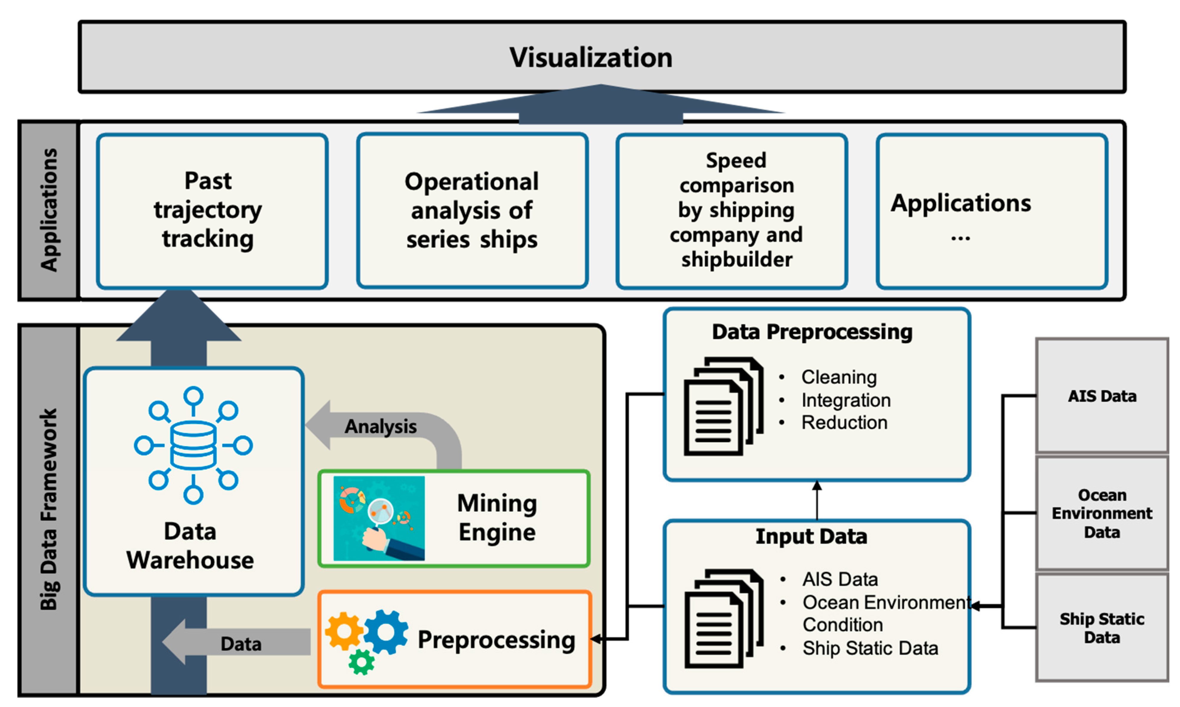
3. Maritime Big Data and the Big Data Handling Framework for Operational Analysis

3.1. Input Data

3.1.1. AIS Data

According to IMO regulations [6,7], all ships are required to carry an automatic identification system (AIS) that automatically provides information on the ship to other ships and coastal authorities. AIS sends 27 messages, including all the information on the ship’s navigation status every few seconds. Among these messages, ‘Message 1′ includes the navigational information, such as the time, course over ground, speed over ground, position, and ‘Message 5′ includes the IMO number of the ship, actual draft, departure, destination, etc. In this study, the analysis was carried out using ‘Messages 1 and 5′. The target ships were 624 container ships operated by 90 shipping companies. The target period was one year from January 2017 to December 2017.

3.1.2. Ocean Environment Data

The ocean environmental conditions can affect the ship’s operation. Therefore, it was necessary to consider the effects of the ocean environment where the ship is sailing. The ocean environment data can be obtained from the global national climatic data center, such as the European Centre for Medium-Range Weather Forecast (ECMWF) [32] and National Oceanic and Atmospheric Administration (NOAA) [33]. The data include the time, latitude, longitude, 10 m U wind component, V wind component, significant wave height with wind waves and swell, wave direction, wave period, surface water temperature, current speed and direction.

3.2. Combining the Maritime Big Data and the Data Handling Framework

The AIS data and ocean environment data can be combined using the time variable. When a certain time is selected, the longitude and latitude of a ship can be obtained from the AIS data. Then, it is possible to collect the ocean environmental information from the ocean environment data using the time and position. As AIS data are saved every few seconds, the size of this database was very large. The data size for the 624 ships analyzed in this study was over 43 GB. Furthermore, the data size for the ocean environment data was much larger. This can differ depending on the resolution of the ocean map and time, but usually it runs into several terabytes per year. It is difficult to collect only the relevant target information from such big data using a normal computing system. In this study, we used the Hortonworks [34] big data framework for the maritime data analysis. Hortonworks provides the Apache Hadoop [30] based big data framework, including related projects for big data analysis. Apache Spark [31] is one of the projects used for data mining and analysis, and Zeppelin [35] is used as a user interface and visualization tool for the analysis.
Figure 1 shows the configuration of the big data framework for operational analysis. The AIS data, ocean environment data, and ship static data such as dimensions, engine specifications and the IMO number were saved. The data included some noise; therefore, cleaning, integration, and reduction processes are necessary as preprocessing. After preprocessing, the relevant, valuable information was obtained according to the applications. Subsequently, the information can be visualized using the developed visualization program described in Section 3.3, or other programs such as Microsoft Excel.

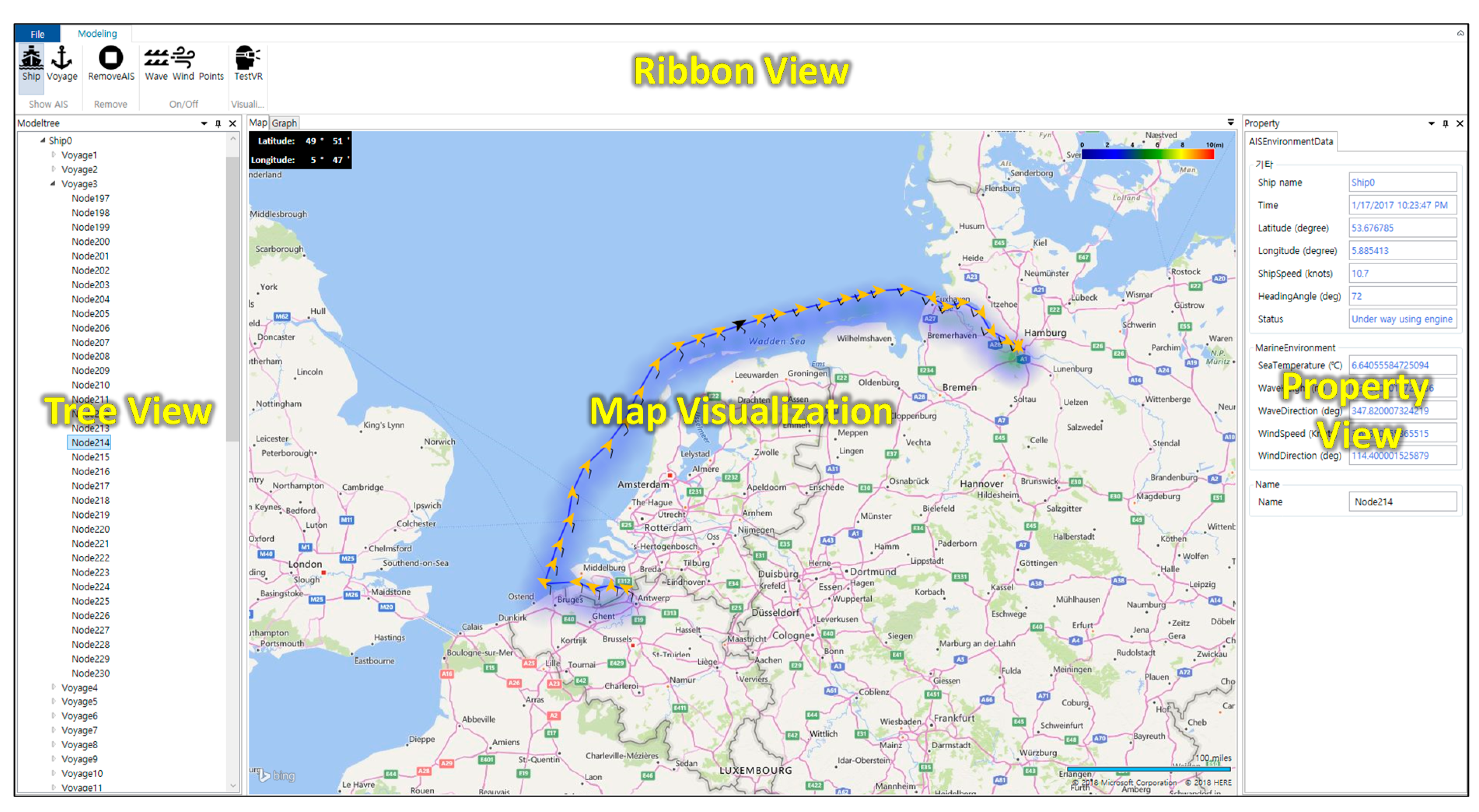
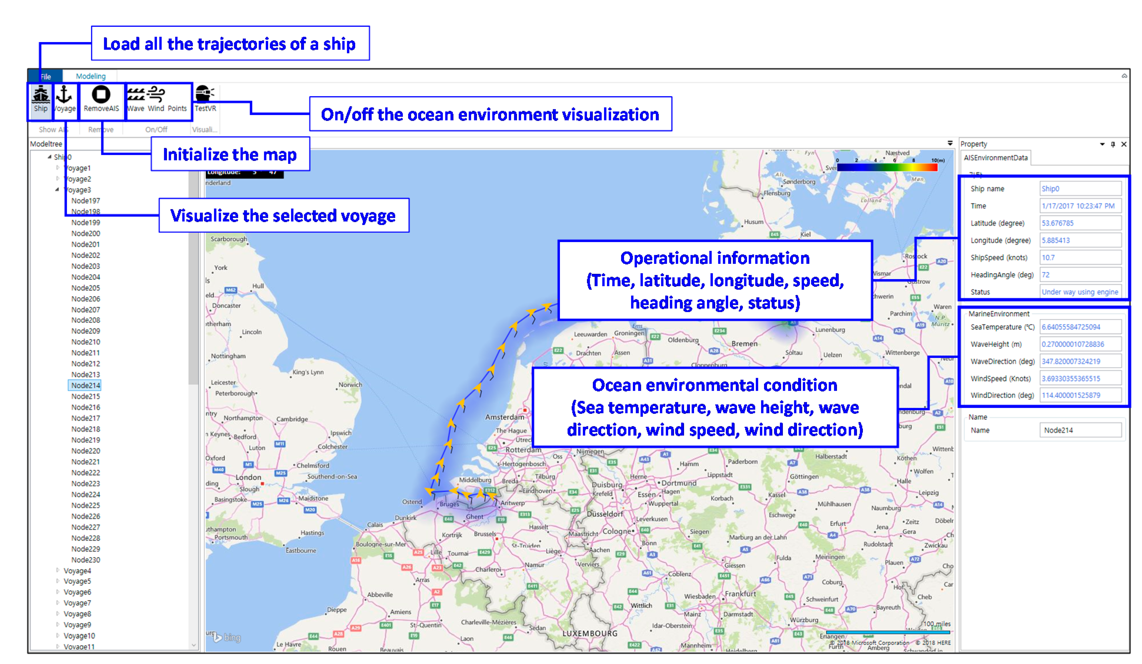
3.3. Visualization Program for Maritime Data Analysis

It is necessary to check the speed, location, and ocean environmental conditions of the target ship at a specific time to analyze the ship’s operational characteristics. In particular, the location of the ship can give rise to different interpretations. If the ship’s speed is slow near the port area, then it is a normal operation. However, if the ship is operating in the middle of the ocean at low speed, there might be a problem on board. Therefore, a visualization tool is necessary to analyze the maritime data. In this study, we developed a visualization program to analyze the ship’s operation, as shown in Figure 2. This consists of a map visualization view, tree view, ribbon view, and property view. The map visualization view shows the trajectory of a ship and the ocean environmental conditions at a certain position using a heat map. The arrow shows the heading angle, and the wind direction and strength were presented using a wind barb symbol, as shown in Figure 3. The wind barb shows the speed and direction using the ‘flag’ on the end. The tree view shows each voyage of a ship and nodes that are at certain positions during the voyage. Additionally, each voyage can be individually selected and visualized. In the property view, the AIS data information, such as time, longitude, latitude, heading angle, speed, wave height, and wind speed and direction, is shown at the selected node. The ribbon view can load AIS data and select the visualization methods.
The visualization program was implemented using C# and WPF (Windows Presentation Foundation) for the graphic user interface, and Microsoft Bing Maps library [36] for the map and color label visualization. This visualization program was used to show the voyage information for the applications in Section 4.

4. Operational Analysis of Container Ships

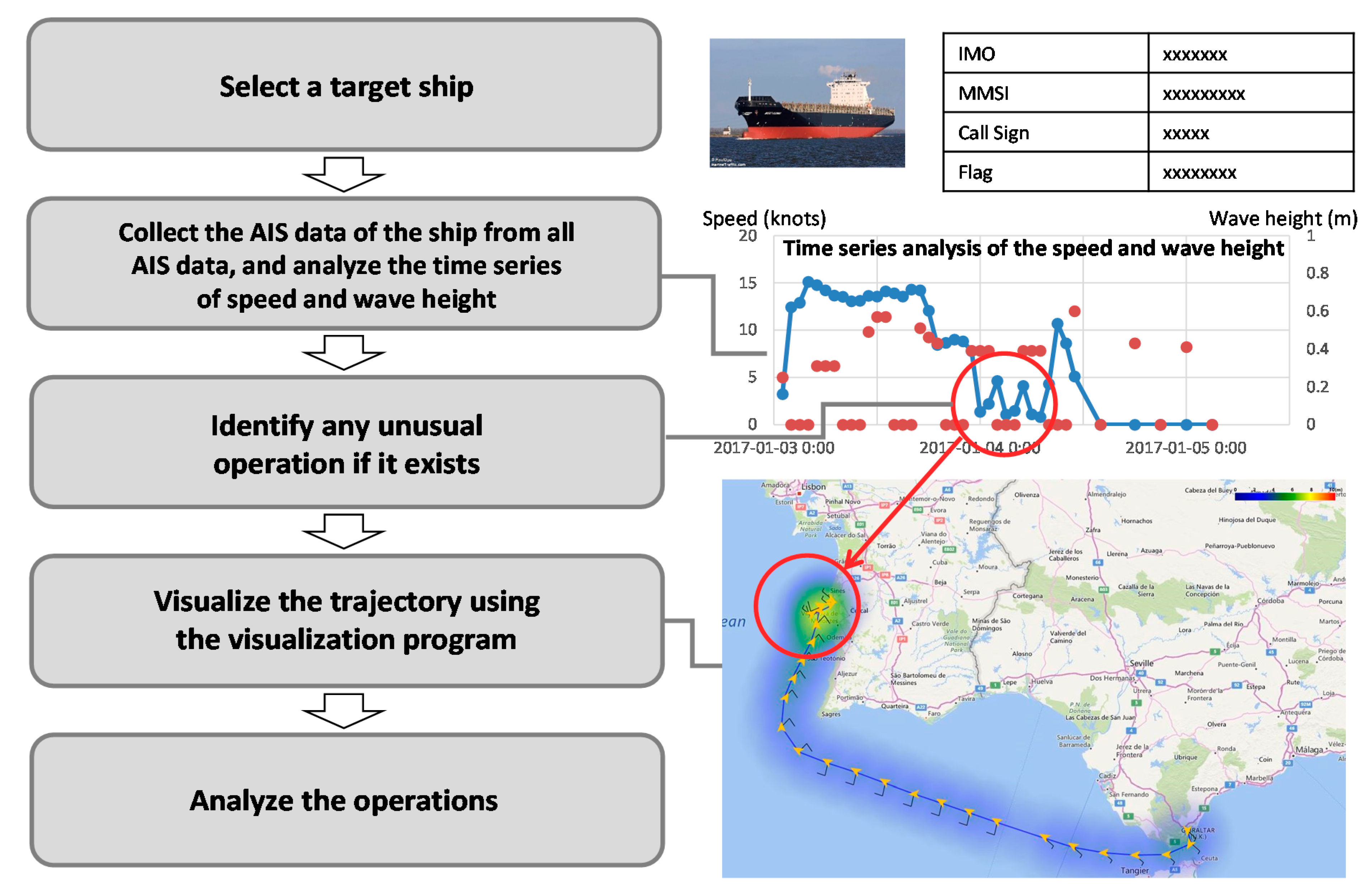
4.1. Trajectory Tracking and Analysis

The overall process of trajectory tracking and analysis is shown in Figure 4. Generally, AIS data include information on all ships. Therefore, it is necessary to first collect the data of the target ship using the big data framework. Thereafter, the details of the voyage can be obtained by analyzing the ship’s status, such as the underway, at anchor, and mooring. Each voyage can be shown in the time series of speed and wave height. From the time series analysis, it is possible to identify any unusual operation if one exists. The voyage data then need to be checked as regards to where the ship sailed and what the wave condition was by using the visualization program proposed in Section 3.3. Finally, we can analyze the operation of the ship. For instance, the ship in Figure 4 was waiting near the port while moving at a very low speed (circled area).

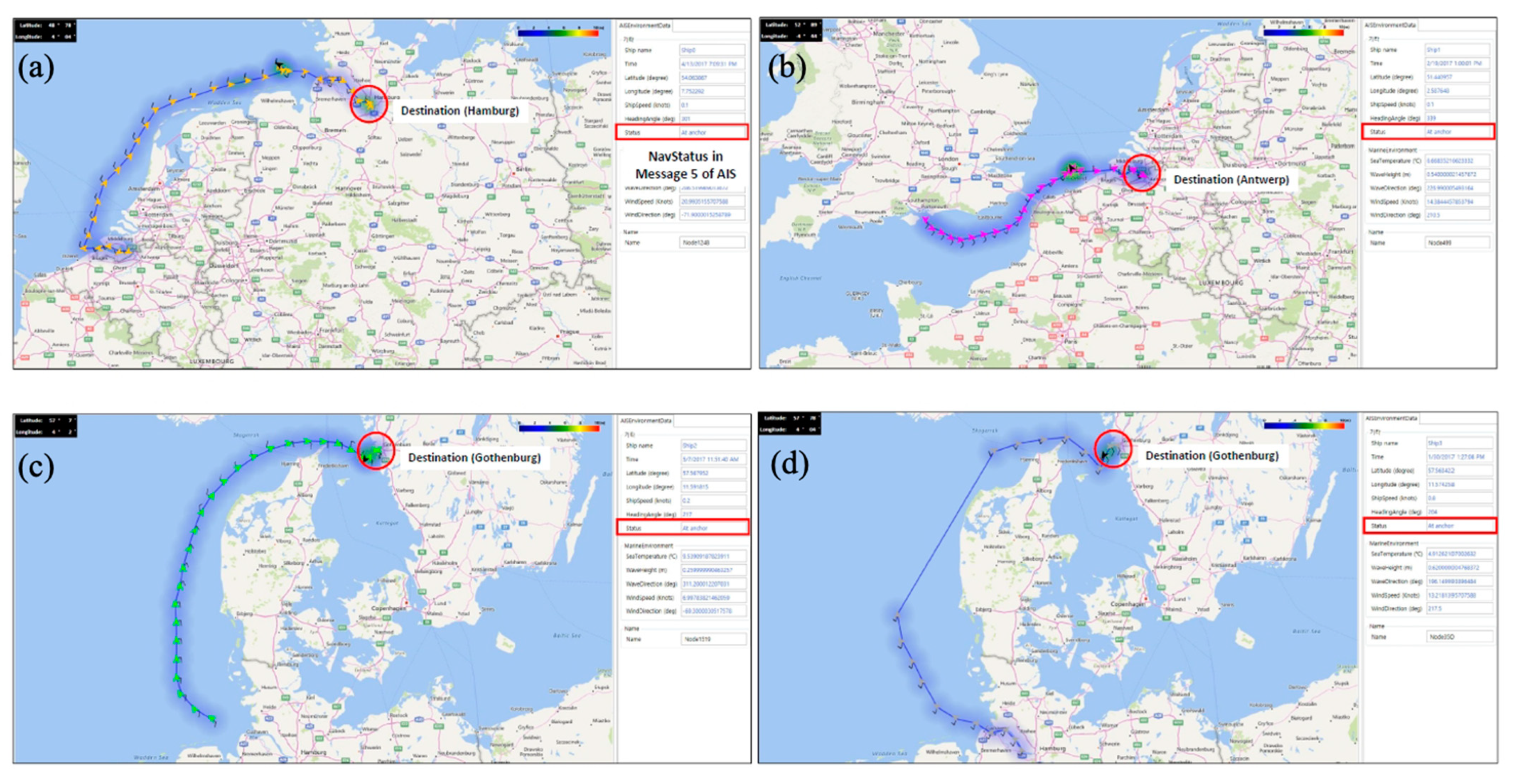
4.1.1. Past Trajectory Tracking of a Container Ship

AIS data contain the positions of ships at a certain time. Therefore, if we track the position of a ship by time, the past routes can be obtained, and it is possible to analyze the operations. Figure 5 shows the previous trajectories of a 10,000 TEU container ship. It departed from Valencia, Spain, and arrived at Duqm, Oman.
Some of the voyages are shown in a time sequence in Figure 6. The first voyage is shown in Figure 6a, in which the ship departed from Valencia and arrived in Algeciras. The average speed was 15.27 knots, and the ship was waiting before entering the port. The wave height was lower than 1 m. Figure 6b shows the second voyage of the container ship. The average speed was 15.11 knots, and the wave height was similar to the first voyage. The ship was waiting near the port (the circled area), and also just before entering the port. Figure 6c shows the long-distance voyage from Sines to Fort Lauderdale. As the ship sailed the transatlantic section, it maintained a very high speed. The average speed was 21.37 knots. The wave condition was good, as shown in the graph.
By analyzing the AIS data and ocean environment data, it was possible to trace the previous trajectories of the container ship. In addition, the operational history could be obtained, such as speed, waiting time, and wave condition. Waiting around the ports was common for all operations. It was impossible to know the stipulated time of arrival, but evidently, the ship arrived before the scheduled time and had to wait before entering the ports. Depending on the routes, the average speeds were different. It was found that the ship sailed at a higher speed on the long-distance route.

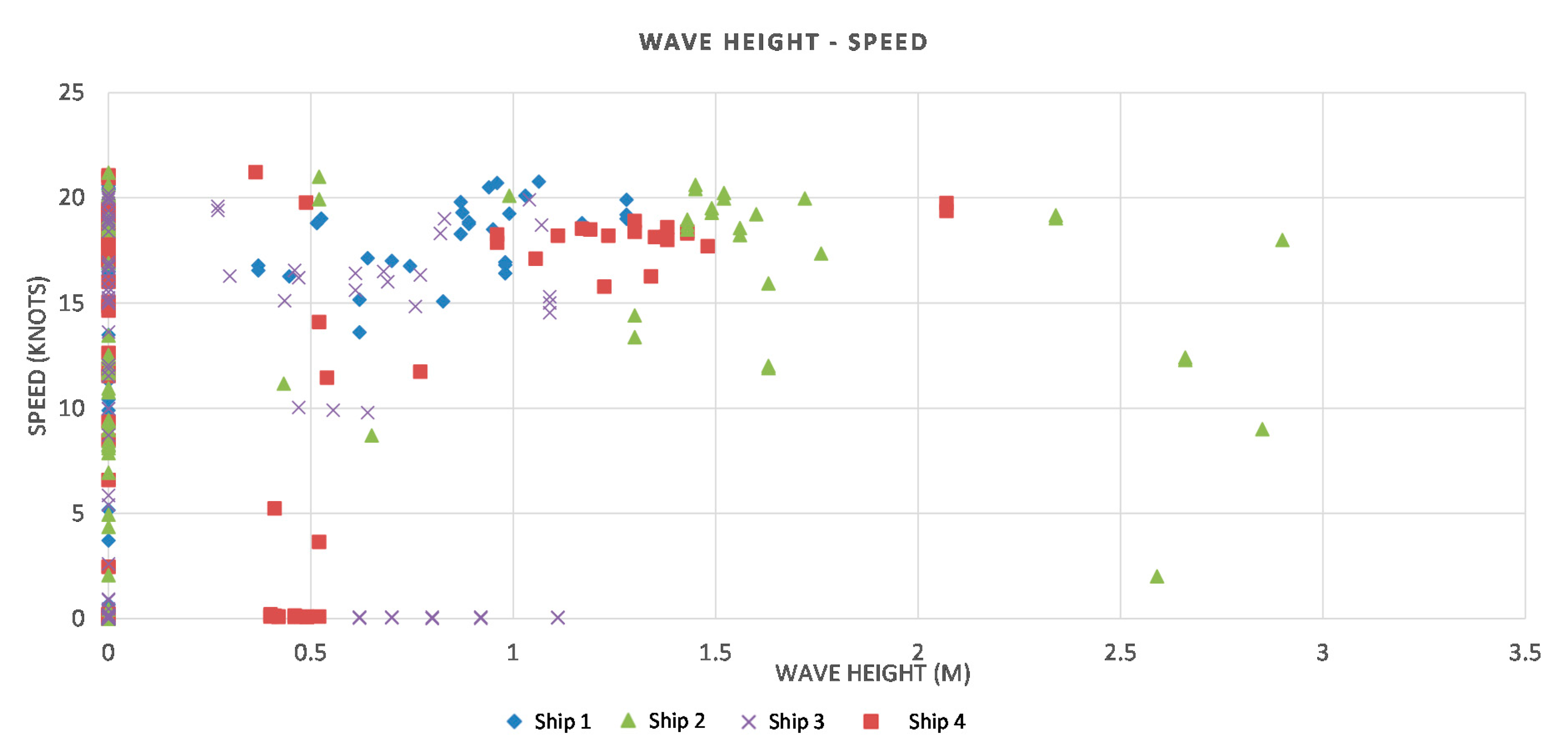
4.1.2. Speed Comparison of a Container Ship for the Same Route

The operating speeds of the same 10,000 TEU container ship in Section 4.1.1 are analyzed for the same routes in this section. Figure 7 shows the operational analysis of the container ship from Sines, Portugal to New York, USA. The sailing time was nine days for all the voyages, but the average speeds were different. Figure 7a shows one voyage for the sailing period from 2 to 11 January 2017. The average speed was 18.64 knots. Figure 7b shows another voyage with the same route. The sailing period was 21 to 30 April 2017, and the average speed was 20.87 knots. One more example of the same route is shown in Figure 7c from 7 to 16 June 2017. The average speed was 17.7 knots. We can assume that the voyage distances were similar, as the ship sailed similar routes. In addition, the wave conditions were good with mostly low wave heights. Although a high wave of approximately 2.5 m height was found in Figure 7a, it was for a short period. Further discussion regarding the ship’s speed and wave height will be presented in Section 4.1.3. By comparing the average speeds during the three voyages, we can deduce that the energy efficiency of the voyage in Figure 7b was not as good as that in the other voyages. Normally, higher ship speed means more fuel oil consumption [37]. Furthermore, for the same sailing period, a higher average speed translates to a longer waiting time near the port. More information regarding the waiting time, such as mooring or anchoring time, will be analyzed in greater detail in Section 4.1.4.
In this section, we compared the speed of a container ship for the same route. The operational pattern may vary depending on the operational status of the port, such as the density of ships simultaneously waiting to enter the port, the stipulated delivery time, and ocean environmental conditions. It was found that even if it took the same number of days for sailing in similar weather conditions, there could be different patterns that affect energy efficiency. From this analysis, it is possible to arrive at the most energy-efficient operational patterns. Furthermore, it can be a benchmark for other competitors.

4.1.3. Operation Comparison among Series Container Ships for the Same Route

The operations of series container ships were compared in this study. As an example, four 13,000 TEU container sister ships that sailed the same route were selected. By analyzing their speed and time graph, we obtained the operational patterns of the series container ships. Figure 8 shows the operational patterns of the series container ships that sailed from Beilun, China to Mawan, China. When we consider the three voyages taking place in the same direction as shown in Figure 8a–c, ship 1 had the lowest average speed, whereas ship 3 had the highest. On the other hand, the sailing time was the longest at three days for ship 3. The wave heights were not very high during the operations except for a short period during ship 2′s voyage when they were almost 3 m. From this comparison, it is clear that ship 3 had the lowest efficiency of operation for the voyage than the others. The ship’s speed was the highest, but it also took the longest time. This means that not only did ship 3 wait a long time near the port, but also consumed more fuel due to its high speed as compared to the other ships.
The worst case is seen in Figure 8d for ship 4, which traveled the same route, albeit in the opposite direction. The voyage took a total of four days, with the lowest average speed of 16.54 knots. However, there was a substantial waiting period before its arrival into port. The average speed was just 2 knots lower, and yet the voyage took two days more. It is clear that the scheduling of the operation was not efficient as compared to the other ships’ voyages. There are some studies [38,39,40] related to the port operations to reduce the waiting time. Generally, it is not easy to calculate the waiting time unless the port provides the estimated waiting time at the arrival. However, it is possible to estimate the waiting time if we have enough data to calculate the average waiting time at the port from the AIS data. Then, it can be possible to optimize the voyage.
It is found that ship 2 encountered the highest wave height of approximately 3 m, and its speed was reduced. We analyzed the relationship between the ship’s speed and the wave height for more voyages on the same route, and the result was shown in Figure 9. In most of the voyages, the waves were not high, but in some cases, the wave heights were more than 2.5 m. Ship 4 operated in over 2.5 m wave heights four times, and one of the operating speeds was about 2.4 knots. Further information is required to find the ship’s status at the operation. More severe weather conditions were not found because normally ships are not operated under harsh environmental conditions on the route. Additionally, the wave height below 3 m does not affect the ship’s speed. It can be concluded that the stipulated time of arrival is a more important factor than the wave height.
In this section, we compared the operations of the series container ships for the same route. Although the ships sailed the same route, the operational patterns were different, and we could observe whether a particular voyage was more efficient or not by comparing it to the other voyages. From this analysis, it is possible to estimate the departure date and average speed when the arrival time is given. For example, ship 4 in Figure 8d could have operated at a lower speed for four days and saved on fuel oil consumption and waiting time. We also analyzed the relationship between the ship’s speed and the wave height. Even though the waves were not very high, no correlation was found. If the wave height is too large, then the ship departs on a different day or changes its route. It can be concluded that the more important factors for speed are the stipulated arrival time and the characteristics of the first officer.

4.1.4. Mooring or Anchoring Time Analysis around Ports

Mooring or anchoring time analysis is one of the applications that can be obtained by trajectory tracking. The AIS data include the ship’s status, such as underway using the engine, at anchor, and mooring. If we find a ship that is anchored or mooring near the port and calculate the time spent in that status, then the mooring or anchoring time can be obtained. We selected four 13,000 TEU container ships to analyze the mooring or anchoring time as an example for analysis. The results are shown in Figure 10.
Ship 4 had the shortest mooring time of 46 h, and ship 3 had the longest mooring time of 75 h. The mooring time can differ depending upon the complexity of the port, but the mooring time should be taken into consideration for efficient operation. For example, ship 3 in Figure 10c waited 28 h more than ship 4 in Figure 10d. Furthermore, it was observed that all the ships chosen for this example waited at least two days before entering the port.
The mooring time can be obtained by analyzing the trajectory tracking and the ship’s status from the AIS data. When a ship is positioned near a port, and its status is mooring or anchoring, it can be assumed that the ship is waiting to enter the port, and the mooring time can be calculated. It is evident that a shorter mooring time is better for efficient operation. It is also used to establish the best schedule considering the overall shipping time and the ship’s speed. By analyzing the mooring time, it is possible to have a more efficient operation.

4.2. Speed Pattern Analysis of Container Ships by Shipping Companies and Shipbuilders

Shipping companies operate their ships according to their unique governing principles. Therefore, the operational characteristics can differ from company to company. For example, if the wave height is high, then the operator may reduce the ship’s speed to achieve lower fuel oil consumption. Sometimes, the operator may maintain a constant speed in spite of bad weather conditions in order to meet the stipulated arrival time. From the point of view of shipyards, it is difficult to know how the ship is operating once the ship is delivered, and how the level of the ship’s performance is decreasing during the operation time. In this study, these operational characteristics regarding the speed on the basis of shipping companies and shipbuilders were analyzed. A total of 624 ships owned by 90 shipping companies were chosen for analysis. The analysis period selected was January to December 2017. The wave conditions from the ocean environment data for that period were used. We selected wave height conditions of 4 m and above to find the operational patterns that emerge because of the relation between speed and harsh environmental conditions.
To obtain the operational characteristics, we applied the very popular data clustering method—k-means clustering [41,42]—to maritime big data. The clustering algorithm is shown in the Appendix A. The overall process of the analysis is shown in Figure 11, and the proposed algorithm is shown as Algorithm A1. A total of 624 container ships were used for the analysis in this study. The container ships were classified by three classes, namely: 8600 TEU; 13,000 TEU; and 18,000 TEU classes. These are the exact sizes of the selected container ships for the analysis. The clustering constraints are the class of the container ship (size), period, and wave height. The analysis period is one year viz. 2017. The 4 m and above wave height are selected as the ocean environmental conditions. We selected these harsh environmental conditions to analyze how the shipping companies operate the ships, and how fast the ships were operated depending on which shipyard built the ship. The number of cluster K is given as three so that we can classify the ship’s speed into low, medium, and high-speed clusters. Among the 624 container ships, the number of clustered ships that were suitable for the given constraints was 491; out of which 274 were 8600 TEU class, 143 were 13,000 TEU class, and 74 were 18,000 TEU class container ships. The results of the analysis will be discussed in the following sections.

4.2.1. Speed Pattern Analysis by Shipping Companies
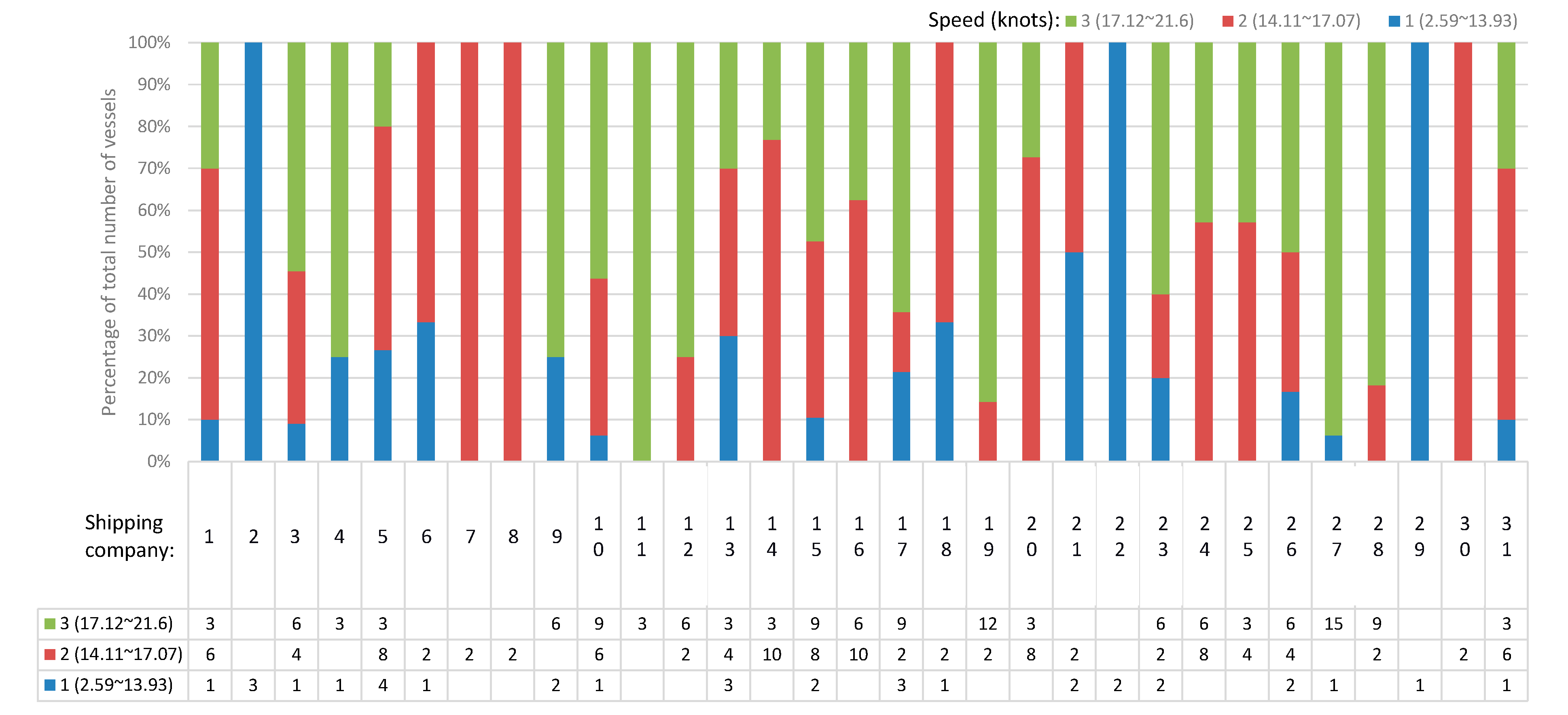
The speed patterns of ships operated by different shipping companies can be analyzed using Algorithm A1. After the clustering, the clustered data can be mapped to the shipping companies. Then, we can analyze how the shipping companies operated the ships in certain conditions. The clustering was done by using the given data. If we already know that the data contain a very small number of ships operated at a certain condition, we can remove them before the analysis. However, it is very difficult to find such information from big data.
1.
Speed pattern analysis of the 8600 TEU container ships operated by different shipping companies
The analysis result of the speed pattern by shipping companies for the 8600 TEU container ships that sailed in 4 m and above wave conditions is shown in Figure 12. As the number of cluster K was given as three, the result shows that the speed groups are 2.59–13.93 knots; 14.11–17.07 knots; and 17.12–21.6 knots. Thirty-one shipping companies were found from the result. This means that the 8600 TEU class container ships owned by 31 companies were operated in 4 m and above wave conditions in 2017. The largest number of ships owned by a single shipping company that sailed in these wave conditions was 19 and were owned by shipping company 15. Most of them had medium to high speeds. The ships that are owned by shipping companies 19, 27, and 28 were operated at very high speed under harsh environmental conditions. The ships that are owned by shipping companies 1, 5, 14, 20, and 31 were operated in the middle-speed range. Some shipping companies with patterns operating at low speeds in a range between 2.59 and 13.93 knots under harsh environmental conditions were found.
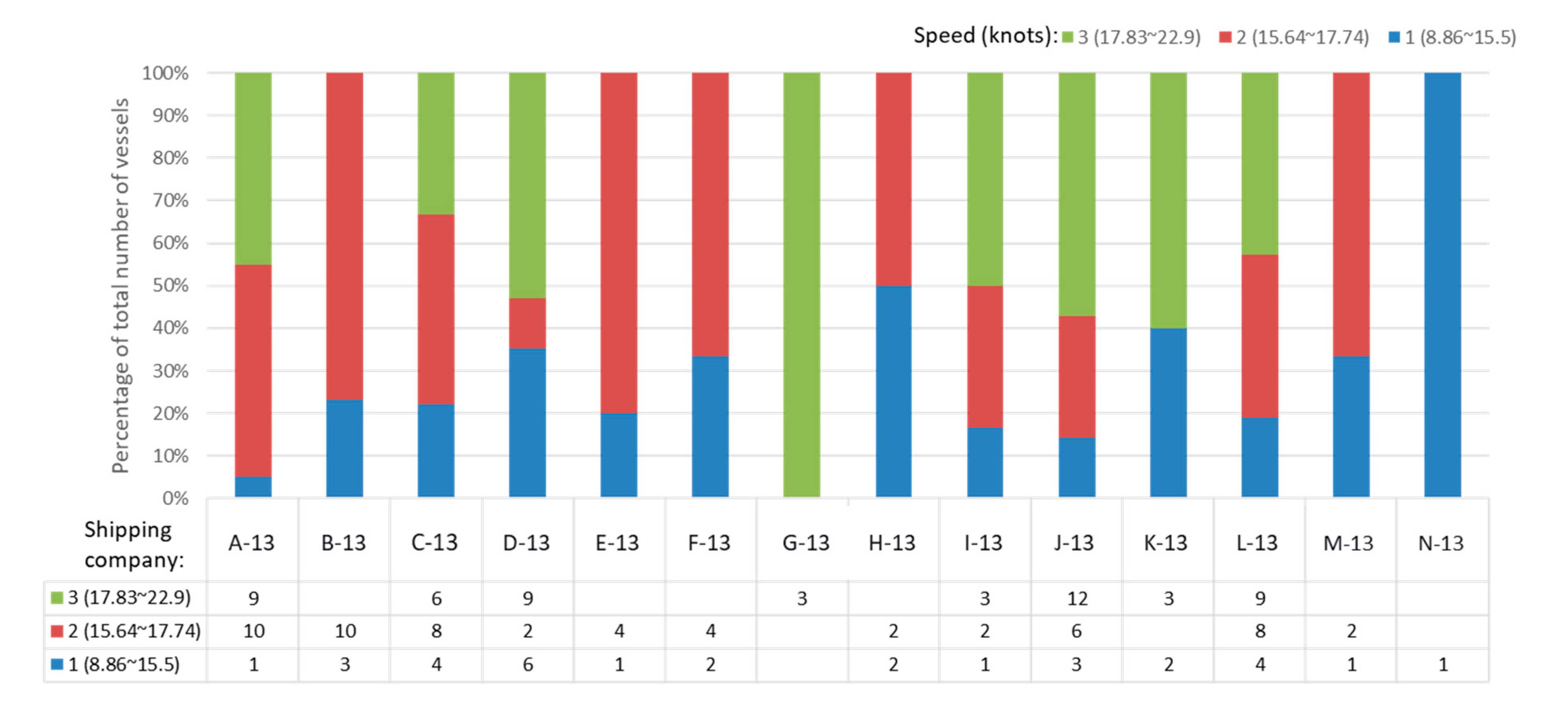
2.
Speed pattern analysis of the 13,000 TEU container ships by different shipping companies
The speed pattern clustering result is shown in Figure 13. Fourteen shipping companies that satisfied the clustering constraints were found. The number of clustering groups here is also three, but the speed values are higher than those for the 8600 TEU container ships. This means that the 13,000 TEU container ships were operated at a higher speed than the 8600 TEU container ships. The ships owned by shipping company D-13 operated at low and high speeds, and the ships owned by company G-13 operated only at high speeds. The ships owned by company B-13 operated at middle speed, and many ships of company J-13 operated at high speeds.
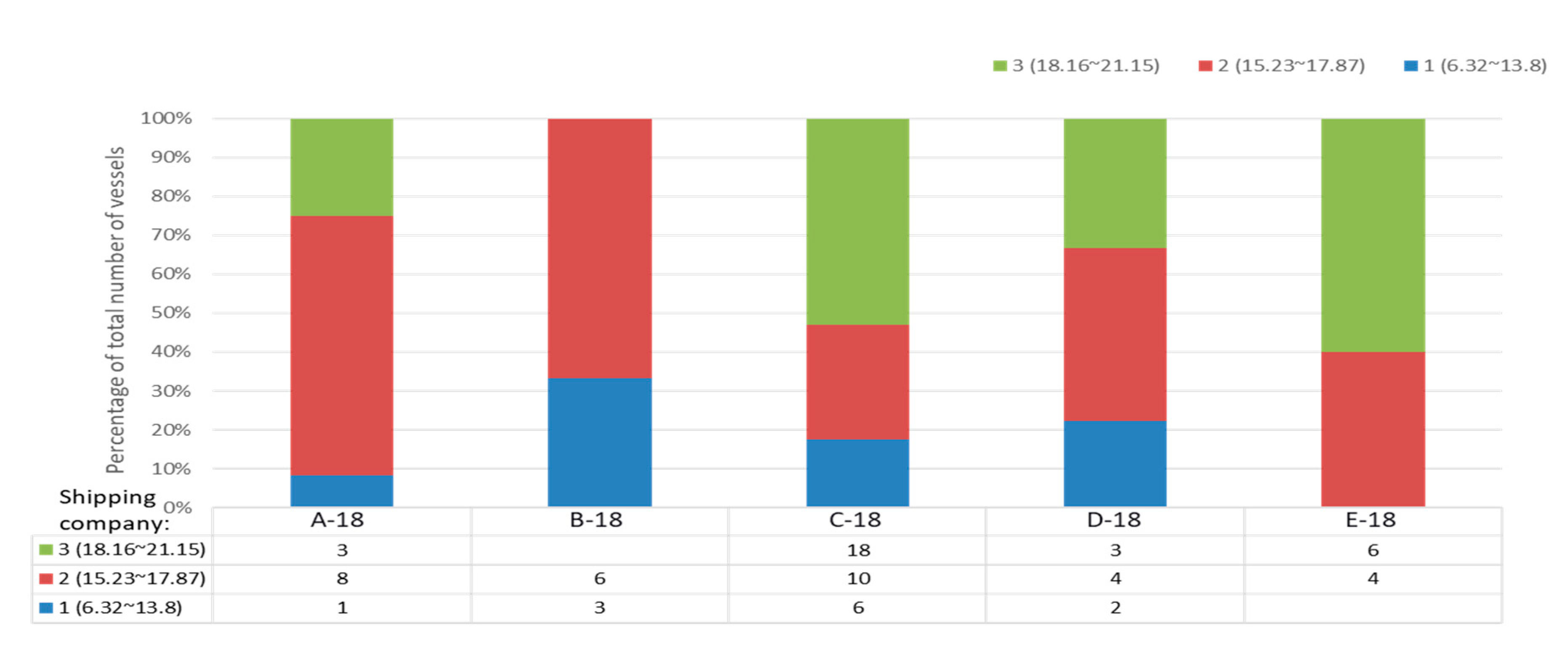
3.
Speed pattern analysis of the 18,000 TEU container ships by shipping companies
The analysis of the speed pattern for 18,000 TEU container ships is shown in Figure 14. It was found that shipping company C-18 owned the most ships among all. Among the ships owned by company C-18, most of them operated at high speeds and middle speeds. The ships owned by company B-18 operated at relatively middle and low speeds, and the ships owned by company E-18 operated at middle and high speeds under the harsh environmental conditions.
From the speed pattern analysis of container ships operated by different shipping companies, we could perceive how the companies operated the ships under harsh environmental conditions. It is well known that if the ship operated at high speed under bad weather conditions, then the fuel oil consumption was high. Therefore, this analysis can be used to decide the economic operation. In this study, we only set the wave condition above 4 m, but for more precise analysis, other constraints should be considered, such as the scheduled time, route, design speed, how long the bad weather continued, etc.

4.2.2. Speed Pattern Analysis by Shipbuilders
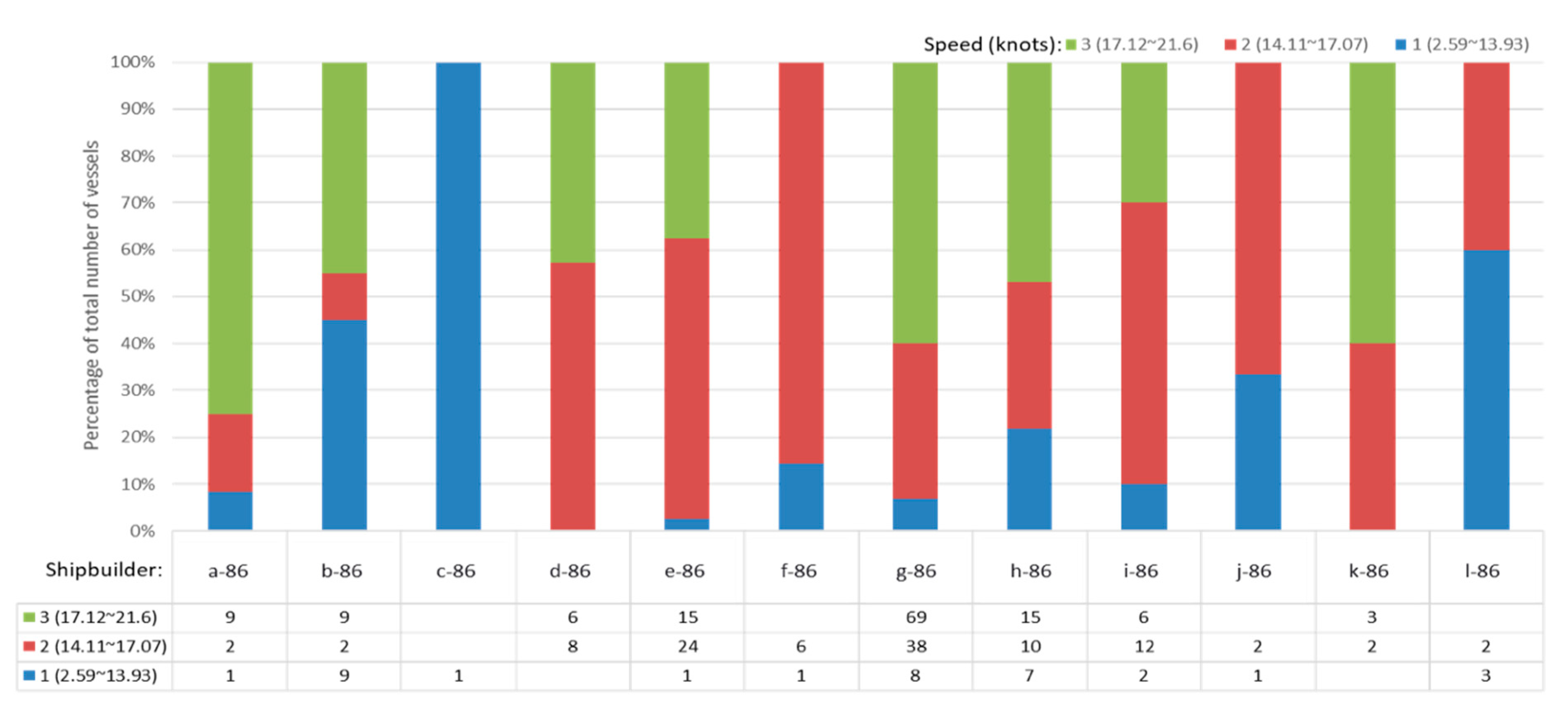
The speed pattern of ships by different shipbuilders can also be analyzed by using Algorithm A1, and the clustered result can be mapped to the shipbuilders. Then, we can evaluate how the ships built by different shipbuilders are operated under the given conditions.
1.
Speed pattern analysis of the 8600 TEU container ships by shipbuilders
From the analysis result in Figure 15, it is observed that shipbuilder g-86 has built the largest number of 8600 TEU class ships, and most of them were operated in a high-speed range from 17.12 to 21.6 knots under the given harsh environmental conditions. The ship’s speed may be affected by the shipping companies’ operational policy, route, weather conditions, and scheduled time, but it can be said that ships from certain shipbuilders can deliver high performance.
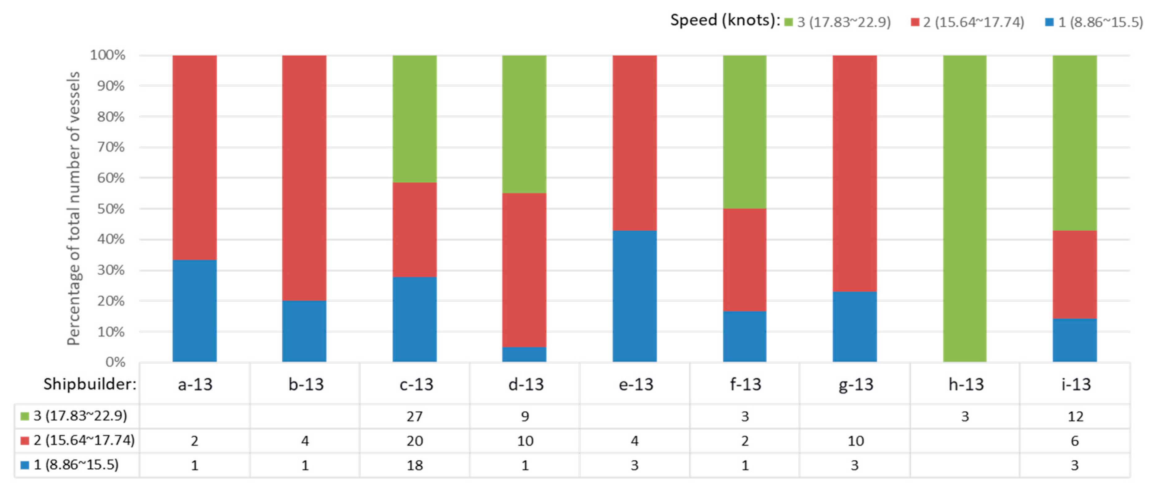
2.
Speed pattern analysis of the 13,000 TEU container ships by shipbuilders
In the case of the 13,000 TEU class container ships (see Figure 16), shipbuilder c-13 built the largest number of ships, and the ships were quite evenly distributed among the three speed clusters. It was also identified that the ships from shipbuilder I can deliver high performance, and the ships from shipbuilder g-13 deliver middle range performance. However, in this case, the other conditions that were discussed in the 8600 TEU analysis result should be considered.
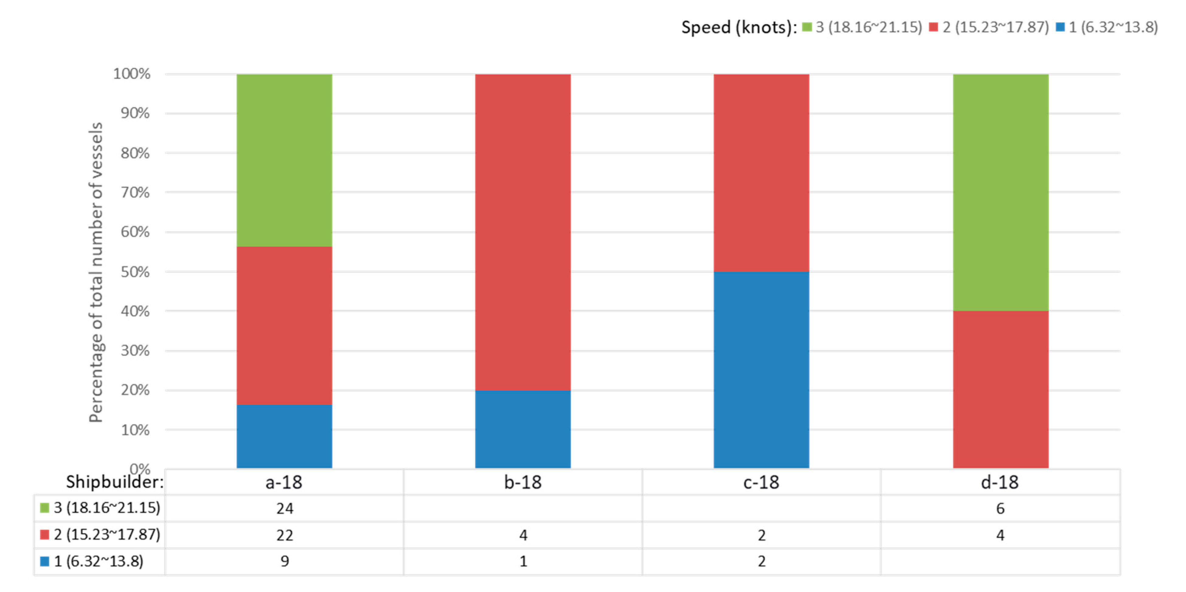
3.
Speed pattern analysis of the 18,000 TEU container ships by the shipbuilders
In the case of the 18,000 TEU class container ships (see Figure 17), we find that shipbuilder a-18 built the largest number of ships. The distributed speed of these ships ranged from the middle to high. The ships from shipbuilder d-18 also have the same speed range, but the ships from the shipbuilders b-18 and c-18 have relatively low-speed range.
In this section, we proposed the speed pattern analysis algorithm analyzed on the basis of shipping companies and shipbuilders. The operational speed patterns of 8600 TEU, 13,000 TEU, and 18,000 TEU class container ships under harsh environmental conditions were analyzed. From this analysis, it was possible to estimate which shipping companies operate their ships fast or slow, and ships built by which shipbuilders are operated at high or low speed in the given constraints. As discussed earlier, other variables do affect the ship’s speed, but it was possible to find which ships were fast or slow in the given 4 m wave height conditions. As it is a relatively harsh wave condition, the ships’ performance can be assumed. If it is not a harsh environmental condition, it is difficult to compare the ship’s performance without the fuel consumption information because more fuel consumption can give higher speed. We can assume that the ships that can operate under harsh environmental conditions with high speed have a good performance. More precise and meaningful results can be obtained if other variables are available, for instance, the scheduled time, route, design speed, how long the bad weather continued, etc. Further study remains with regard to the analysis of the speed, considering the shipbuilders and shipping companies simultaneously.

5. Conclusions and Future Work

The method of the operational analysis of container ships from maritime big data was presented in this study. In this study, maritime data such as the AIS data, ocean environment data, and ship’s static data were used for the analysis of operations. The main contribution of this study was that the AIS data and the ocean environment data were combined, and some applications were proposed by analyzing the combined maritime big data using the big data framework. A big data framework suited to process the big size of maritime data was proposed, and the data handling procedure was explained. We also developed the visualization program essential for analyzing the container ship’s operation. The program can present the AIS data and ocean environment data simultaneously based on time. We proposed past trajectory tracking, the speed comparison of different container ships for the same route, operation comparison among series ships for the same route, and mooring or anchoring time analysis as possible trajectory tracking and analysis applications. Furthermore, the speed pattern analysis by shipping companies and shipbuilders are performed using the k-means clustering method, and the operational patterns of shipping companies and the performance of shipbuilders were obtained. The results were obtained by analyzing the maritime big data. The trajectory tracking and analysis can be used to estimate the transportation cost because the route, speed, and ocean environmental condition can be obtained from the maritime big data to calculate the fuel oil consumption [43]. By comparing the operations of container ships, it can be possible to evaluate the efficiency of transportation and give the insight to identify problems related to the current operations. For example, if it is found that the ship’s speed is decreasing by the speed pattern analysis proposed in Section 4.2.1 with the fuel consumption analysis, the hull cleaning [44] or new build can be considered. If it is found that there is too much waiting time around the ports by the analysis proposed in Section 4.1.3, the owner can take some solutions to reduce the waiting time. Additionally, the proposed method is useful to the other owners or shipbuilders who do not have the operational data of the other ships. The speed pattern analysis proposed in Section 4.2.2 can be a factor in selecting the best shipbuilding company that can make efficient ships for owners. Additionally, the shipbuilding companies can take the technology development to obtain better performance than the other competitors from the analysis. This study focuses on the methods to evaluate the performance of the container ships using AIS data. We proposed estimating the performance of the ships using the public data and how to figure out the operational efficiency, such as the sailing and waiting patterns. To optimize the speed and waiting times at the port, more and different types of data such as the ocean environment conditions and fuel oil consumptions for many years should be collected and analyzed using the proposed methods. The ship owners and shipbuilders may have different analysis results and can take different actions to the results accordingly.
In this study, we only used the one-year data to determine the speed patterns of shipping companies and shipyards. If we selected a target ship and applied the proposed method to the accumulated maritime big data for many years, the degradation of operational performance could be detected. The proposed methods demonstrated how to handle the maritime big data and collect valuable information from the data. It was expected that this study will help make the operations of container ships more efficient. That is, ship operators can have better guidelines if the proposed method was used as the additional indicator to increase the operational efficiency of the ship. However, in fact, the proposed method can be useful to shipyards, service companies, and others who cannot obtain private operational data. They can provide suitable services to the owners for better operational efficiency.
We only used some information in the AIS data for the applications, such as the time, position, and ship’s status, but there is much more information in the AIS data. For instance, AIS data include the actual draft data. Through the draft analysis [10], it could be possible to analyze the world trade volume by container ships. Therefore, more applications using additional information in AIS data can be developed with further studies. Additionally, we plan to make an effort to find the mathematical models that exist in data analysis and to apply this kind of analysis to various problems in the design of ships and offshore structures [45].

Author Contributions

Conceptualization, M.-J.O., S.-W.P. and M.-I.R.; methodology, M.-J.O., S.-W.P. and M.-I.R.; software, M.-J.O., S.-W.P. and D.-H.C.; validation, M.-J.O., S.-W.P., M.-I.R., D.-H.C., M.-J.S. and J.-Y.L.; formal analysis, M.-J.O., S.-W.P., M.-I.R. and D.-H.C.; investigation, M.-J.O. and M.-I.R.; resources, M.-I.R.; data curation, S.-W.P. and D.-H.C.; writing—original draft preparation, M.-J.O.; writing—review and editing, M.-I.R.; visualization, S.-W.P. and D.-H.C.; supervision, M.-I.R.; project administration, M.-I.R.; funding acquisition, M.-I.R. All authors have read and agreed to the published version of the manuscript.

Funding

This work was partially supported by (a) Korean Register, Republic of Korea; (b) MSIP (Ministry of Science, ICT and Future Planning), Republic of Korea, under ‘Development of Ship Design Standard PLM Platform based on Big Data’ (NIPA-2016-S1106-16-1025) supervised by the NIPA (National IT Industry Promotion Agency); (c) Research Institute of Marine Systems Engineering of Seoul National University, Republic of Korea; and (d) Institute of Engineering Research of Seoul National University, Republic of Korea.

Acknowledgments

This work is an expansion of our previous study [46,47].

Conflicts of Interest

The authors declare no conflict of interest. The funders had no role in the design of the study; in the collection, analyses, or interpretation of data; in the writing of the manuscript, or in the decision to publish the results.

Appendix A

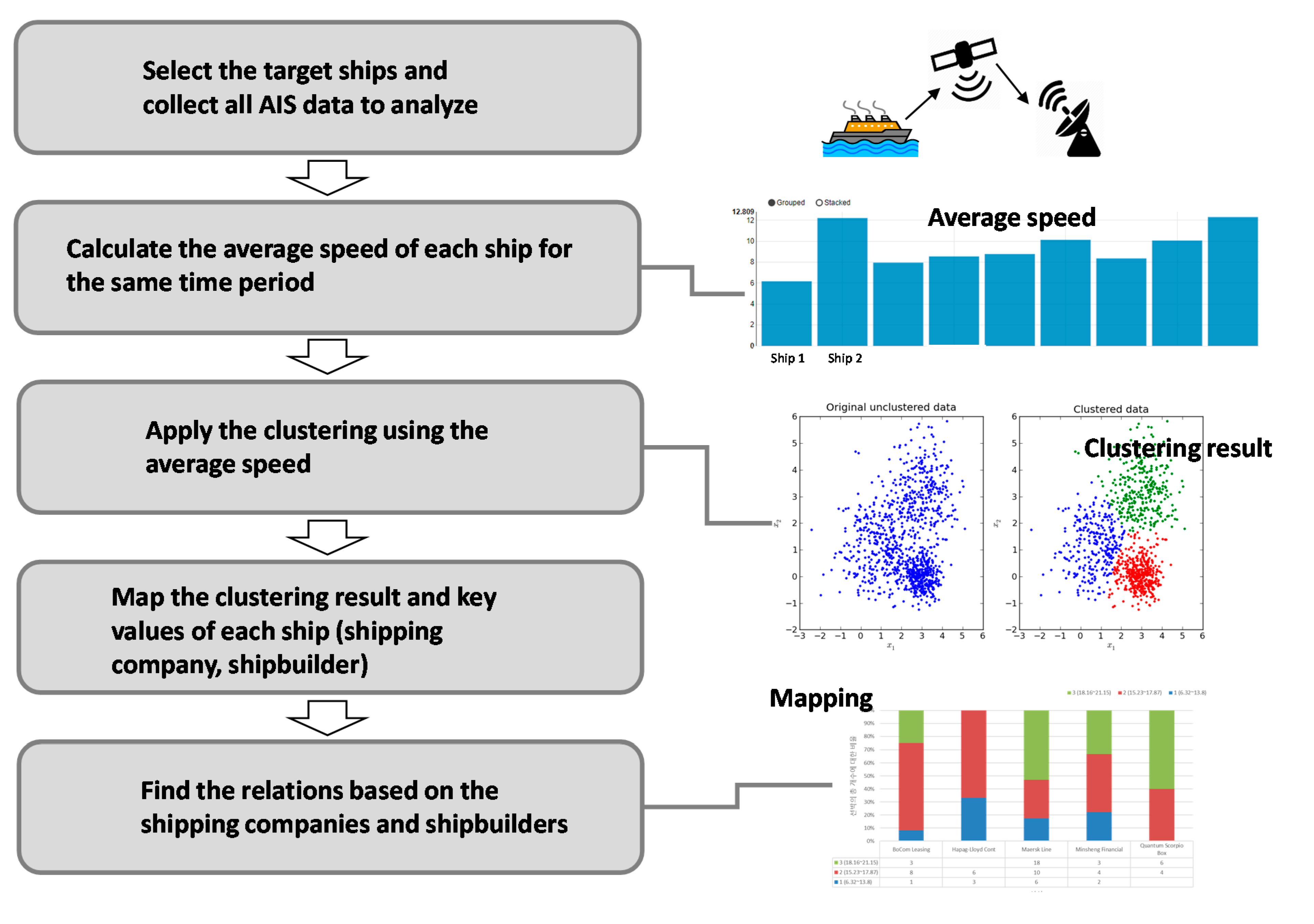
Algorithm A1. Speed pattern analysis of container ships by shipping companies and shipbuilders using the K-means clustering.
Data: AIS data of container ships, ocean environment data, and ship static data
Result: Clustering of the speeds by shipping companies or shipbuilders
Initialize:
Select the target ships;
Select the target period;
Select the target ocean environmental condition;
Clustering:
Select the number of clusters K;
Calculate the average speed of each ship for the period;
Initial speed of clusters ← Randomly select K distinct data by the average speed of a ship;
while Clusters change do
   foreach Average speed of each ship do
     Measure the difference between the initial speed of clusters and the given data;
     Assign the given data to the nearest cluster;
     Calculate the mean speed of each cluster;
     Initial speed of clusters ← mean speed of clusters;
   end
end
Map the clustered speed data to the shipping companies or shipbuilders in the ship static data;

References

  1. Bell, M.G.H.; Meng, Q. Special issue in transportation research part B—Shipping, port and maritime logistics. Transp. Res. Part B Methodol. 2016, 93, 697–699. [Google Scholar] [CrossRef]
  2. Vejvar, M.; Lai, K.H.; Lo, C.K.Y. A citation network analysis of sustainability development in liner shipping management: A review of the literature and policy implications. Marit. Policy Manag. 2020, 47, 1–26. [Google Scholar] [CrossRef]
  3. Le, L.T.; Lee, G.; Kim, H.; Woo, S.H. Voyage-based statistical fuel consumption models of ocean-going container ships in korea. Marit. Policy Manag. 2020, 47, 304–331. [Google Scholar] [CrossRef]
  4. Kim, S.H.; Roh, M.I.; Oh, M.J.; Park, S.W.; Kim, I.I. Estimation of ship operational efficiency from AIS data using big data technology. Int. J. Nav. Archit. Ocean Eng. 2020, 12, 440–454. [Google Scholar] [CrossRef]
  5. Yuen, K.F.; Wang, X.; Ma, F.; Lee, G.; Li, X. Critical success factors of supply chain integration in container shipping: An application of resource-based view theory. Marit. Policy Manag. 2019, 46, 653–668. [Google Scholar] [CrossRef]
  6. International Maritime Organization. SOLAS Chapter V Safety of Navigation; International Maritime Organization: London, UK, 2002. [Google Scholar]
  7. International Maritime Organization. Guidelines for the Installation of a Shipborne Automatic Identification System (AIS); International Maritime Organization: London, UK, 2003. [Google Scholar]
  8. Yang, D.; Wu, L.; Wang, S.; Jia, H.; Li, K.X. How big data enriches maritime research—A critical review of Automatic Identification System (AIS) data applications. Transp. Rev. 2019, 39, 755–773. [Google Scholar] [CrossRef]
  9. Jia, H.; Lampe, O.D.; Solteszova, V.; Strandenes, S.P. An automatic algorithm for generating seaborne transport pattern maps based on AIS. Marit. Econ. Logist. 2017, 19, 619–630. [Google Scholar] [CrossRef]
  10. Jia, H.; Prakash, V.; Smith, T. Estimating vessel payloads in bulk shipping using AIS data. Int. J. Shipp. Transp. Logist. 2019, 11, 25–40. [Google Scholar] [CrossRef]
  11. Perera, L.P.; Carvalho, J.P.; Guedes Soares, C. Fuzzy logic based decision making system for collision avoidance of ocean navigation under critical collision conditions. J. Mar. Sci. Technol. 2011, 16, 84–99. [Google Scholar] [CrossRef]
  12. Wen, Y.; Huang, Y.; Zhou, C.; Yang, J.; Xiao, C.; Wu, X. Modelling of marine traffic flow complexity. Ocean Eng. 2015, 104, 500–510. [Google Scholar] [CrossRef]
  13. Sang, L.; Wall, A.; Mao, Z.; Yan, X.; Wang, J. A novel method for restoring the trajectory of the inland waterway ship by using AIS data. Ocean Eng. 2015, 110, 183–194. [Google Scholar] [CrossRef] [Green Version]
  14. Dobrkovic, A.; Iacob, M.-E.; van Hillegersberg, J. Using machine learning for unsupervised maritime waypoint discovery from streaming AIS data. In Proceedings of the 15th International Conference on Knowledge Technologies and Data-Driven Business—i-KNOW ′15, Graz, Austria, 21–23 October 2015; Association for Computing Machinery: New York, NY, USA, 2015; pp. 1–8. [Google Scholar]
  15. Dobrkovic, A.; Iacob, M.E.; Van Hillegersberg, J. Maritime pattern extraction from AIS data using a genetic algorithm. In Proceedings of the 2016 IEEE International Conference on Data Science and Advanced Analytics (DSAA), Montreal, QC, Canada, 17–19 October 2016; pp. 642–651. [Google Scholar]
  16. Xiao, F.; Ligteringen, H.; van Gulijk, C.; Ale, B. Comparison study on AIS data of ship traffic behavior. Ocean Eng. 2015, 95, 84–93. [Google Scholar] [CrossRef] [Green Version]
  17. Wu, X.; Mehta, A.L.; Zaloom, V.A.; Craig, B.N. Analysis of waterway transportation in Southeast Texas waterway based on AIS data. Ocean Eng. 2016, 121, 196–209. [Google Scholar] [CrossRef]
  18. Zhang, W.; Goerlandt, F.; Montewka, J.; Kujala, P. A method for detecting possible near-miss ship collision from AIS data. Ocean Eng. 2016, 107, 60–69. [Google Scholar] [CrossRef]
  19. Yu, J.; Tang, G.; Song, X.; Yu, X.; Qi, Y.; Li, D.; Zhang, Y. Ship arrival prediction and its value on daily container terminal operation. Ocean Eng. 2018, 157, 73–86. [Google Scholar] [CrossRef]
  20. Wu, X.; Rahman, A.; Zaloom, V.A. Study of travel behavior of vessels in narrow waterways using AIS data—A case study in sabine-neches waterways. Ocean Eng. 2018, 147, 399–413. [Google Scholar] [CrossRef]
  21. Svanberg, M.; Santén, V.; Hörteborn, A.; Holm, H.; Finnsgård, C. AIS in maritime research. Mar. Policy 2019, 106, 10352. [Google Scholar] [CrossRef]
  22. Liu, C.; Liu, J.; Zhou, X.; Zhao, Z.; Wan, C.; Liu, Z. AIS data-driven approach to estimate navigable capacity of busy waterways focusing on ships entering and leaving port. Ocean. Eng. 2020, 218, 108215. [Google Scholar] [CrossRef]
  23. Yan, Z.; Xiao, Y.; Cheng, L.; He, R.; Ruan, X.; Zhou, X.; Li, M.; Bin, R. Exploring AIS data for intelligent maritime routes extraction. Appl. Ocean Res. 2020, 101, 102271. [Google Scholar] [CrossRef]
  24. Wu, X.; Roy, U.; Hamidi, M.; Craig, B.N. Estimate travel time of ships in narrow channel based on AIS data. Ocean. Eng. 2020, 202, 106790. [Google Scholar] [CrossRef]
  25. Yan, Z.; Xiao, Y.; Cheng, L.; Chen, S.; Zhou, X.; Ruan, X.; Li, M.; He, R.; Ran, B. Analysis of global marine oil trade based on automatic identification system (AIS) data. J. Transp. Geogr. 2020, 83, 102637. [Google Scholar] [CrossRef]
  26. Vettor, R.; Guedes Soares, C. Characterisation of the expected weather conditions in the main European coastal traffic routes. Ocean Eng. 2017, 140, 244–257. [Google Scholar] [CrossRef]
  27. Kepaptsoglou, K.; Fountas, G.; Karlaftis, M.G. Weather impact on containership routing in closed seas: A chance-constraint optimization approach. Transp. Res. Part C Emerg. Technol. 2015, 55, 139–155. [Google Scholar] [CrossRef]
  28. Tsou, M.-C. Online analysis process on automatic identification system data warehouse for application in vessel traffic service. Proc. Inst. Mech. Eng. Part M J. Eng. Marit. Environ. 2016, 230, 199–215. [Google Scholar] [CrossRef]
  29. Mao, S.; Tu, E.; Zhang, G.; Rachmawati, L.; Rajabally, E.; Huang, G.-B. An Automatic Identification System (AIS) database for maritime trajectory prediction and data mining. In Proceedings of the ELM-2016, Adaptation, Learning and Optimization, Singapore, 13–15 December 2016; Springer: Cham, Switzerland, 2016; pp. 241–257. [Google Scholar]
  30. Apache Hadoop. Apache Hadoop. 2019. Available online: http://hadoop.apache.org/ (accessed on 25 April 2019).
  31. Apache Spark. Apache SparkTM—Unified Analytics Engine for Big Data. 2019. Available online: https://spark.apache.org/ (accessed on 25 April 2019).
  32. ECMWF. ECMWF|Advancing Global NWP through Co-Operation. Available online: http://www.ecmwf.int/ (accessed on 25 April 2019).
  33. National Oceanic and Atmospheric Administration (NOAA). U.S Department of Commerce. Available online: https://www.noaa.gov/ (accessed on 17 April 2021).
  34. Hortonworks. Data Management Platform, Solutions and Big Data Analysis|Hortonworks. 2018. Available online: https://hortonworks.com/ (accessed on 25 April 2019).
  35. Apache Zeppelin. 2019. Available online: http://zeppelin.apache.org/ (accessed on 25 April 2019).
  36. Microsoft. Custom Maps API for Business|Bing Maps for Enterprise. 2019. Available online: https://www.microsoft.com/en-us/maps/default (accessed on 25 April 2019).
  37. Psaraftis, H.N.; Kontovas, C.A. Speed models for energy-efficient maritime transportation: A taxonomy and survey. Transp. Res. Part C 2013, 26, 331–351. [Google Scholar] [CrossRef]
  38. Ilie, A.; Oprea, C.; Olteanu, S.; Dinu, O.; Ruscǎ, F. An heuristic model for port optimization. Procedia Manuf. 2019, 32, 975–982. [Google Scholar] [CrossRef]
  39. Shahpanah, A.; Poursafary, S.; Shariatmadari, S.; Gholamkhasi, A.; Zahraee, S.M. Optimization waiting time at berthing area of port container terminal with hybrid Genetic Algorithm (GA) and Artificial Neural Network (ANN). Adv. Mater. Res. 2014, 902, 431–436. [Google Scholar] [CrossRef]
  40. Sheikholeslami, A.; Ilati, G.; Yeganeh, Y.E. Practical solutions for reducing container ships’ waiting times at ports using simulation model. J. Mar. Sci. Appl. 2013, 12, 434–444. [Google Scholar] [CrossRef]
  41. Forgy, E.W. Cluster analysis of multivariate data: Efficiency versus interpretability of classifications. Biometrics 1965, 21, 768–769. [Google Scholar]
  42. MacQueen, J. Some methods for classification and analysis of multivariate observations. In Proceedings of the 5th Berkeley Symposium on Mathematical Statistics and Probability, Berkeley, CA, USA, 21 June–18 July 1965 and 27 December 1965 and 7 January 1966; University of California Press: Berkley, CA, USA, 1967; pp. 281–297. [Google Scholar]
  43. Schinas, O.; Stefanakos, C.N. Cost assessment of environmental regulation and options for marine operators. Transp. Res. Part C Emerg. Technol. 2012, 25, 81–99. [Google Scholar] [CrossRef]
  44. Adland, R.; Cariou, P.; Jia, H.; Wolff, F.C. The energy efficiency effects of periodic ship hull cleaning. J. Clean. Prod. 2018, 178, 1–13. [Google Scholar] [CrossRef]
  45. Oh, M.J.; Roh, M.I.; Park, S.W.; Chun, D.H.; Myung, S.H. Big data-based piping material analysis framework in offshore structure for contract design. Ocean Syst. Eng. 2019, 9, 79–95. [Google Scholar]
  46. Oh, M.J.; Roh, M.I.; Park, S.W.; Chun, D.H.; Lee, J.Y.; Son, M.J. Operational analysis of container ships using AIS data. In Proceedings of the ACDDE 2018, Okinawa, Japan, 1–3 November 2018; pp. 1–5. [Google Scholar]
  47. Oh, M.J.; Roh, M.I.; Park, S.W.; Chun, D.H.; Son, M.J. Operational analysis of container ships using AIS data based on big data technology. In Proceedings of the Annual Autumn Conference, The Society of Naval Architects of Korea, Changwon, Korea, 8–9 November 2018; p. 218. [Google Scholar]
Figure 1. Configuration of the big data framework for operational analysis.
Jmse 09 00438 g001
Figure 2. Visualization program.
Jmse 09 00438 g002
Figure 3. Functions and information of the AIS data and ocean environment data on the visualization program.
Jmse 09 00438 g003
Figure 4. Trajectory analysis process.
Jmse 09 00438 g004
Figure 5. Trajectory analysis of a container ship.
Jmse 09 00438 g005
Figure 6. Analysis of the previous trajectories with ocean environmental conditions in Figure 5. (a) Voyage 1, 1~2 January, 2017, (b) Voyage 2, 3~4 January, 2017, (c) voyage 3, transatlantic route, from 5 to 13 January, 2017.
Jmse 09 00438 g006
Figure 7. Operational analysis of the 10,000 TEU container ship for the same route from Sines, Portugal to New York, USA. (a) 2~11 January, 2017 (9 days), average speed 18.64 knots, (b) 21~30 April, 2017 (9 days), average speed 20.87 knots, (c) 7~16 June, 2017 (9 days), average speed 17.7 knots.
Jmse 09 00438 g007
Figure 8. Past operation comparison for the series container ships. (a) Voyage of the ship 1, 27~29 December, 2017 (2 days), average speed 17.49 knots, (b) Voyage of the ship 2, 15~17 December, 2017 (2 days), average speed 18.25 knots, (c) Voyage of the ship 3, 12~15 November, 2017 (3 days), 18.77 knots, (d) Voyage of the ship 4, 24~28 November, 2017 (4 days), average speed 16.54 knots.
Jmse 09 00438 g008
Figure 9. Analysis of the ship’s speed and the wave height.
Jmse 09 00438 g009
Figure 10. Mooring time analysis of 13,000 TEU container ships. (a) Ship 1, mooring period: 13~15 April, 2017 (46 h), (b) Ship 2, mooring period: 19~21 February, 2017 (60 h), (c) Ship 3, mooring period: 7~10 May, 2017 (75 h), (d) Ship 4, mooring period: 30 January~1 February, 2017 (47 h).
Jmse 09 00438 g010
Figure 11. Process of the ship’s speed pattern analysis by shipping companies and shipbuilders.
Jmse 09 00438 g011
Figure 12. Speed clustering results of the 8600 TEU container ships by shipping companies.
Jmse 09 00438 g012
Figure 13. Speed clustering result of the 13,000 TEU container ships by shipping companies.
Jmse 09 00438 g013
Figure 14. Speed clustering result of the 18,000 TEU container ships by shipping companies.
Jmse 09 00438 g014
Figure 15. Speed clustering result of the 8600 TEU container ships by shipbuilders.
Jmse 09 00438 g015
Figure 16. Speed clustering result of the 13,000 TEU container ships by shipbuilders.
Jmse 09 00438 g016
Figure 17. Speed clustering result of the 18,000 TEU container ships by shipbuilders.
Jmse 09 00438 g017
Table 1. Summary of the related works and this study.
StudyInput DataApplicationAlgorithmBig Data
Jia et al. [10] (2019)AIS dataBulk ship payloads estimationRegressionNo
Kim et al. [4] (2020)AIS data and ocean environment dataOperational efficiency estimationOwn algorithmYes
Liu et al. [22] (2020)AIS dataNavigable capacity of waterways estimationK-means clusteringNo
Yan et al. [23] (2020)AIS dataMaritime routes extractionGraph theoryNo
Wu et al. [24] (2020)AIS dataTravel time estimation in narrow channelOwn algorithmNo
Yan et al. [25] (2020)AIS dataOil trade analysisOwn algorithmNo
This studyAIS data and ocean environment dataOperation analysisData mining, K-mean clusteringYes
Publisher’s Note: MDPI stays neutral with regard to jurisdictional claims in published maps and institutional affiliations.

