Experimental Study on Development of Mooring Simulator for Multi Floating Cranes

Abstract

In this study, the coupled motion of a mooring system and multifloating cranes were analyzed. For the motion analysis, the combined equations of motions of the mooring line and multifloating cranes were introduced. The multibody equations for floating cranes were derived from the equations of motion. The finite element method (FEM) was used to derive equations to solve the stretchable catenary problem of the mooring line. To verify the function of mooring simulator, calculation results were compared with commercial mooring software. To validate the analysis results, we conducted an experimental test for offshore operation using two floating crane models scaled to 1:40. Two floating crane models and a pile model were established for operation of uprighting flare towers. During the model test, the motion of the floating cranes and tensions of the mooring lines were measured. Through the model test, the accuracy of the mooring analysis program developed in this study was verified. Therefore, if this mooring analysis program is used, it will be possible to perform a mooring analysis simulation at the same time as a maritime work simulation.

1. Introduction

There has been the need to perform dynamic analysis of mechanical systems. Consequently, several simulation tools that focus on traditional mechanical systems, such as automobiles and robots, have been developed. In recent years, the need for motion analysis in the shipbuilding industry has been increasing.

However, shipbuilding and offshore industries generally differ from conventional mechanical systems in terms of purpose, size, and shape. Therefore, there are limits to the application of analysis tools developed for existing mechanical systems in the shipbuilding and offshore industries. For this reason, simulation tools were developed in several studies for the dynamic analysis of shipbuilding and offshore operation processes [1,2]. In the previously developed simulation program, the multibody dynamics theory is applied to perform a more accurate dynamic analysis of crane operations on the sea. However, mooring lines are defined as linear springs in most programs, and spring constants are determined based on some assumptions and linearization. However, for some offshore operations, such as installation and decommissioning, mooring analysis may be a vital point of analysis. Therefore, in this paper, the following research was conducted in relation to mooring analysis.

• The mooring analysis module was implemented by referring to the existing research results [3].
• This mooring analysis module has been integrated with the multibody dynamics module that we have previously developed [1,2].
• A model test was conducted to verify the performance of the integrated program.

The other parts of this paper are organized as follows. In Section 2, previous studies related to this study are reviewed, and the scope of the study is defined. Section 3 describes the equations for motion analysis of multifloating crane and mooring line. Section 4 shows the comparison between simulation results of the developed simulator and commercial program, and Section 5 describes the model test results for the verification of the developed program. Section 6 presents a summary of this study and briefly describes a future related study.

2. Related Studies

Several studies on mooring line analysis have been conducted. In the research of Garrett, D.L., and Kim, B.W., the motion of the vessel and the mooring system are analyzed simultaneously, called the fully coupled method [4,5,6]. The equations of motion are formulated for both the floating body and the mooring line. Numerical models and procedures provide accurate and efficient global modeling, and the analysis results are more accurate than the simulation results obtained using the linear spring methods. However, in these studies, the floating structure is modelled as a single body, which is not capable of simulating offshore operation of floating cranes.

On the other hand, Ham, S.H., and Cha., J.H. present the simulation methods for offshore operation of floating cranes [7,8]. In these studies, the floating crane was modelled as a multibody, which has joints that can simulate the motion of offshore cranes. However, the mooring line was assumed as a linear spring line for the motion analysis. For this assumption, the determination of the spring constant is crucial. Moreover, the complicated motion of the mooring line was approximated based on the linear spring model, so the results of the analysis cannot be sufficiently precise for some aspects, in spite of the reduced simulation time [9,10].

Recently, Gutiérrez-Romero, J.E. presented the nonlinear dynamic FEM mooring model to analyze the response of moored floating wind turbines [11]. In this research, a FEM mooring module was implemented, and the floating wind turbine was modeled as a multibody, so that this research carried out an accurate simulation. However, to model the wind turbine, Gutiérrez-Romero, J.E. used FAST, which can be used only for wind turbine analysis. So, we cannot use the result of this research for analysis of floating cranes.

On the other hand, as the need for an accurate analysis of the dynamic behavior in shipbuilding and offshore industries has increased, we developed a floating crane simulation tool in previous research [1,2]. The programs developed from these studies were based on multibody dynamics, and more sophisticated motions of vessels and cranes can be simulated. Therefore, we decided that the simulation tool is suitable for simulation of offshore operations using floating cranes and planned to integrate the mooring analysis module developed in this study into the simulation tool. 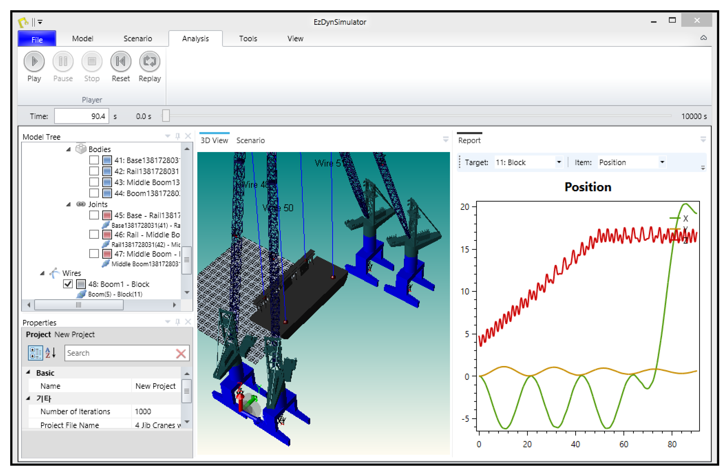Figure 1 shows an example of the GUI program and its application.

Therefore, in this research, we implemented nonlinear mooring analysis module by referring to the existing research results [3]. For simultaneous analysis of mooring line and multibody floating cranes, the interface between the mooring analysis module and existing floating crane simulation tools was designed and implemented. To validate the developed simulator, a model test was conducted.

The input and output data for the static analysis are listed in

Table 1. Input and output data for mooring analysis.

Input Data	Output Data
Mooring line specification - Length of mooring line - Weight of mooring line per meter - Young’s modulus - Section area For FEM Analysis - Stiffness of seabed - Coefficient of Coulomb friction - Number of elements - Start point of mooring line: anchoring position - End point of mooring line: fairlead position on floating body	Line tension Line position

.

3. Equations Used for Simulation Program

For motion analysis of the moored floating crane, the equations of motion for the floating cranes were derived based on multibody dynamics, and the concept of the constrained force was applied. The mooring line was assumed to be stretchable catenary and modeled as a finite element. In this section, the equations of motion used for motion analysis are described.

3.1. Equations of Motion for Floating Crane

All of the floating crane systems in operation are multibody systems, in which multiple rigid bodies are joined. Thus, a dynamic analysis module for the multibody system was developed in this study. The computer methods used in the automated dynamic analysis of multibody systems that consist of rigid bodies are generally divided into two main approaches [12,13]. In the first approach, the system configuration is identified using a set of Cartesian coordinates that describe the locations and orientations of the bodies. This approach is called the “augmented formulation” [14]. In the second approach, relative joint variables are used to formulate a minimum set of differential equations of motion, and two types of formulation use relative joint variables: embedding formulation and recursive formulation. The augmented formulation has the disadvantage of increasing the equation of motion according to the number of objects, but the analysis result is intuitive and has the advantage of calculating the constrain force. Because of this advantage, in this study, the augmented formulation, expressed as Equation (1), was used [13,15].

$$\{\begin{array}{c}\overline{M}\left(q\right)\ddot{q}+C_q^T\left(q\right)\lambda =\overline{F}\left(q,\dot{q}\right)-\overline{k}\left(q,\dot{q}\right)\\ \mathbf{C}\left(q\right)=0 \end{array}$$

(1)

$$\overline{M}\left(q\right)=J{\left(q\right)}^{T}MJ\left(q\right)$$

(2)

$$\overline{F}\left(q, \dot{q}\right)=J{\left(q\right)}^{T}F\left(q, \dot{q}\right)$$

(3)

$$\overline{k}\left(q, \dot{q}\right)=J{\left(q\right)}^{T}M\dot{J}\left(q\right)\dot{q}+J{\left(q\right)}^{T}N\left(\dot{q}\right)J\left(q\right)\dot{q}$$

(4)

where $q$ is the generalized coordinate matrix, $\lambda$ is the constraint force matrix, $C\left(q\right)$ is the constraint matrix, $J\left(q\right)$ is the velocity transformation matrix, $M$ is the mass and inertia matrix, $F$ is the external force matrix, and $N$ is the three-dimensional transformation matrix.

A Newton–Euler equation can be expressed simply based on the center of gravity. However, since a general mechanical system uses a generalized coordinate system in consideration of the user’s convenience, coordinate transformation is necessary, and Equations (2)–(4) shows the process of performing this coordinate transformation, which is calculated by multiplying $J{\left(q\right)}^T \mathrm{and} J\left(q\right)$ on $M, F, \mathrm{and} N$ [15].

3.2. Equations of Motion for Mooring Line

An analytical solution of the nonstretchable catenary mooring line has been provided [16]. In this study, however, the mooring line was assumed to be stretchable, and several numerical solutions of the problem are available. Among the previous studies, the equation derived by Kim was adopted in this study [3]. In this research, the mooring line was divided into several elements to model the mooring line, and Equation (5) was derived by integrating the equations of each element. The equation for static analysis using the FEM is expressed as follows:

$$\left[K\right]\left\{u\right\}=\left\{f_{\mathrm{n}}\right\}+\left\{f\right\}$$

(5)

where u is the position of the node for each finite element. By solving this static equation, the static equilibrium position, tension, and mooring forces can be calculated. Each term in Equation (5) is presented as follows:

$$\left[K\right]={\displaystyle \sum }_e\left[\begin{array}{cc}\left[K_{ge}\right]& \left\{D_g\right\}\\ {\left\{D_g\right\}}^T& \left\{Z\right\}\end{array}\right]$$

(6)

$$\left\{Z\right\}=-\frac{s_0}{EA}$$

(7)

where $s_0$ is the initial length of each finite element of the mooring line, $E$ is Young’s modulus of the mooring line, and $A$ is the section area of the mooring line.

$$\left\{D_g\right\}={\left[R\right]}^T\left\{D\right\}$$

(8)

$$\left\{D\right\}=\left\{B\right\}+\left[C\right]\left\{u_e\right\}$$

(9)

$$\left\{B\right\}=\frac{2}{J+1}{\left[-100100\right]}^T$$

(10)

$$\left\{u_e\right\}=\left[R\right]\left\{u_{ge}\right\}$$

(11)

In Equations (8)–(11), $u_{ge}$ is the global position of the node for each finite element, $R$ is the transformation matrix that transforms the global vector to a local vector, and $u_e$ is the local position of the node for each finite element.

$$\left[K_{ge}\right]={\left[R\right]}^T\left[K_e\right]\left[R\right]$$

(12)

$$\left[K_e\right]=\lambda \left[C\right]$$

(13)

$$\left[C\right]=\frac{1}{\left(J+1\right)l}\left[\begin{array}{cc}\begin{array}{ccc}1& 0& 0\\ & 1& 0\\ & & 1\end{array}& \begin{array}{ccc}-1& 0& 0\\ 0& -1& 0\\ 0& 0& -1\end{array}\\ \begin{array}{ccc} & & \\ S& y& m\\ & & \end{array}& \begin{array}{ccc} 1 & 0& 0\\ m & 1& 0\\ & & 1\end{array}\end{array}\right]$$

(14)

$$J=\sqrt{{\left(1+u_x^{\prime }\right)}^2+u_y^{\prime }{}^2+u_z^{\prime }{}^2}$$

(15)

$$\left\{u\right\}=\left\{\begin{array}{c}\left\{u_{ge}\right\}\\ \lambda \end{array}\right\}$$

(16)

$$\left\{f_n\right\}={\displaystyle \sum }_e\left\{\begin{array}{c}-\left\{f_{we}\right\}\\ s_0-l\end{array}\right\}$$

(17)

$$\left\{f_{we}\right\}=\frac{Jwl}{2}{\left[001001\right]}^T$$

(18)

In Equations (12)–(18), $\lambda$ is the Lagrange multiplier, $l$ is the distance between the local coordinates, and $w$ is the weight of the unit length of the mooring line. B, C, and D are symbols used to simplify the equation. B stands for Equation (10), C stands for Equation (14), and D stands for Equation (9). The Newton–Rapson method was adopted to solve Equation (5) [17].

3.3. Definition of Interface between Modules

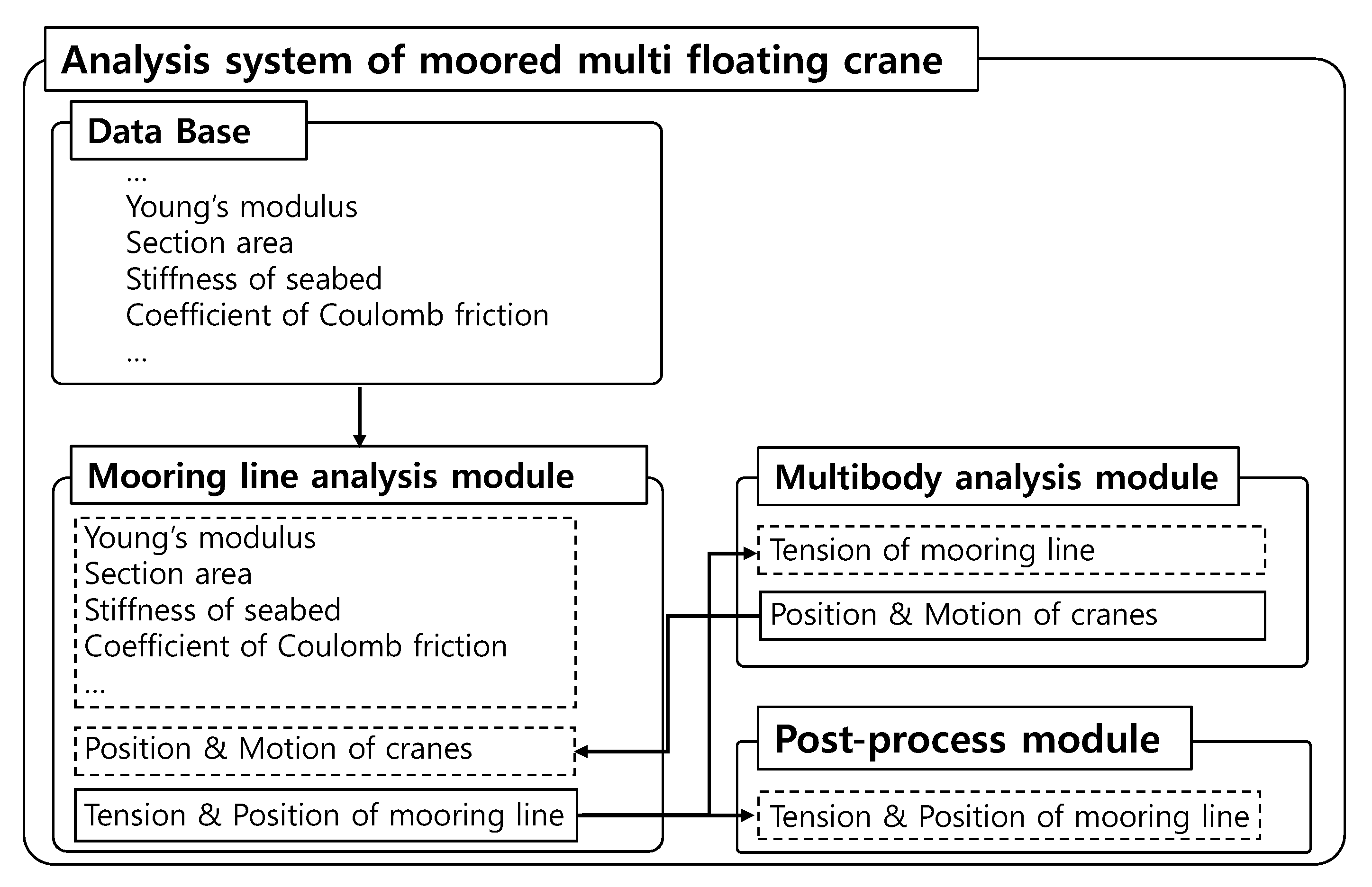
The multibody analysis module and the mooring line analysis module are independent of each other because their governing equations are different. Therefore, the analysis modules should translate the mooring information to each other. For the translation, an interface between two modules has been developed. The interface and input/output details are depicted in Figure 2. This figure shows only limited information exchanged between the mooring analysis module and the multibody analysis module targeted in this paper.

The mooring line and multibody analysis modules are integrated in the analysis program of the moored multifloating crane, and the mooring line analysis module exchanges the data with a database, a multibody analysis module, and a postprocessing module.

The mooring line analysis module receives the following types of information from the database:

-

physical information about the mooring line;

-

physical information about the seabed.

The mooring line analysis module receives the following types of information from the multibody analysis module:

-

position, velocity, and acceleration information about the multifloating cranes.

The mooring line analysis module provides the following types of information to the multibody analysis module and postprocessing module.

-

tension (mooring force) is provided to the multibody analysis module;

-

tension (mooring force), position, and shape of the mooring rope are provided to the postprocessing module.

4. Verification of Mooring Line Analysis Module

As mentioned in the previous chapter, the mooring line and multibody analysis modules are integrated in the analysis program. Among them, the multibody analysis modules were developed and verified in previous research [15]. To verify the mooring line analysis module, we conducted several simulations of mooring examples. The example in Section 4.1 is referenced in [3], and the example in Section 4.2 is an example of pulling test of floating mass made up in this study. The calculation results were compared with [3] and a commercial program for mooring analysis called Orcaflex, respectively, to verify the calculation accuracy of the module developed in this paper.

4.1. Verification Examples of Static Analysis

In the previous section, equations for analysis were presented. In this section, a static analysis solver was developed first, and for verification, the simulation results and the nonstretchable analytic solution, which is described in research [3], were compared. An example of a mooring line is shown in Figure 3. To make the mooring line nonstretchable in the developed solver, Young’s modulus was set as infinite number. Figure 4 shows the comparison results. In the graph, the line represents the simulation results obtained using the developed solver, and the dots represent the analytical solution—they are the same.

Figure 5, Figure 6, Figure 7 and Figure 8 show the static equilibrium position and tension for the same example. The slope angle q varies from 0° to 60°, where q is the angle between the x-axis and dotted linear line L. The analysis results depict a parabolic catenary curve shape. As the axial stiffness, which is proportional to EA, decreases, the sag increases quadratically, and the tension of the mooring line decreases, which indicates that the mooring force also decreases. These results were compared with other research [3], and they were the same. Therefore, we could confirm that the stretchable mooring line analysis function is accurate enough to use.

The calculation process described above is performed without considering the bottom reaction of the sea. However, the mooring line is generally in contact with the seabed. In addition, mooring lines in contact with the seabed have a significant effect on mooring performance; hence, the bottom condition must be considered. The method of considering the ground conditions in the analysis module was applied as follows:

$$k_c\{\begin{array}{c}0(z>z_c)\\ w_c/{\delta }_c(z<z_c)\end{array}$$

(19)

$$c_c\{\begin{array}{c}0(z>z_c)\\ 2{\epsilon }_c\sqrt{m_c{k}_c}(z<z_c)\end{array}$$

(20)

where $z$ is the height of the mooring node, $z_c$ is the seabed depth, $k_c$ is the seabed stiffness, $w_c$ is the weight of the mooring node, ${\delta }_c$ is the penetration depth of the mooring line, $c_c$ is the damping coefficient of the seabed, ${\epsilon }_c$ is the damping ratio, and $m_c$ is the weight of the mooring node.

The contact force of the seabed was computed using the above equation. An example of the mooring line is shown in Figure 9, Figure 10 and Figure 11, which depict the static equilibrium position and tension of the numerical example. The slope angle q was varied from 20° to 60°. The analysis results show a parabolic catenary curve shape. The sag increases quadratically with a decrease in the axial stiffness (the axial stiffness is proportional to EA). Moreover, the tension of the mooring line decreases with the axial stiffness, which suggests that the mooring force also decreases.

4.2. Verification Examples of Pulling Test

In this section, a performed simulation of pulling test for evaluating the function of the mooring line analysis module is described. The example of the simulation is shown in Figure 12. This example was made up for comparison with commercial programs. It is possible to calculate the restoration force generated by the mooring line by moving the point mass, and through this, we can assess whether it is the same as the calculation performance of the verified commercial program.

For each of the two cases, the floating bodies were forced to move from −55 to +55 m. The tension of wire rope was calculated, a restoring force curve was plotted, and the simulation results were compared with those of OrcaFlex [18]. The simulation conditions for Case 1 and Case 2 are outlined as follows.

A. Case 1

• Vertical distance between anchor and floating body: 300 m.
• Horizontal distance from anchor to floating body: 600 m.
• Unstretched length of mooring line: 690 m.
• Stiffness EA: 500 and 700 MN.

B. Case 2

• Vertical distance between anchor and floating body: 500 m.
• Horizontal distance from anchor to floating body: 866 m.
• Unstretched length of mooring line: 1026 m.
• Stiffness EA: 500 and 700 MN.

Figure 13 shows the calculated restoring force. The solid line represents the simulation results obtained using the analysis module developed in this study, while the dotted line represents the simulation results obtained using Orcaflex. It can be observed that the simulation results are almost the same.

5. Experimental Study

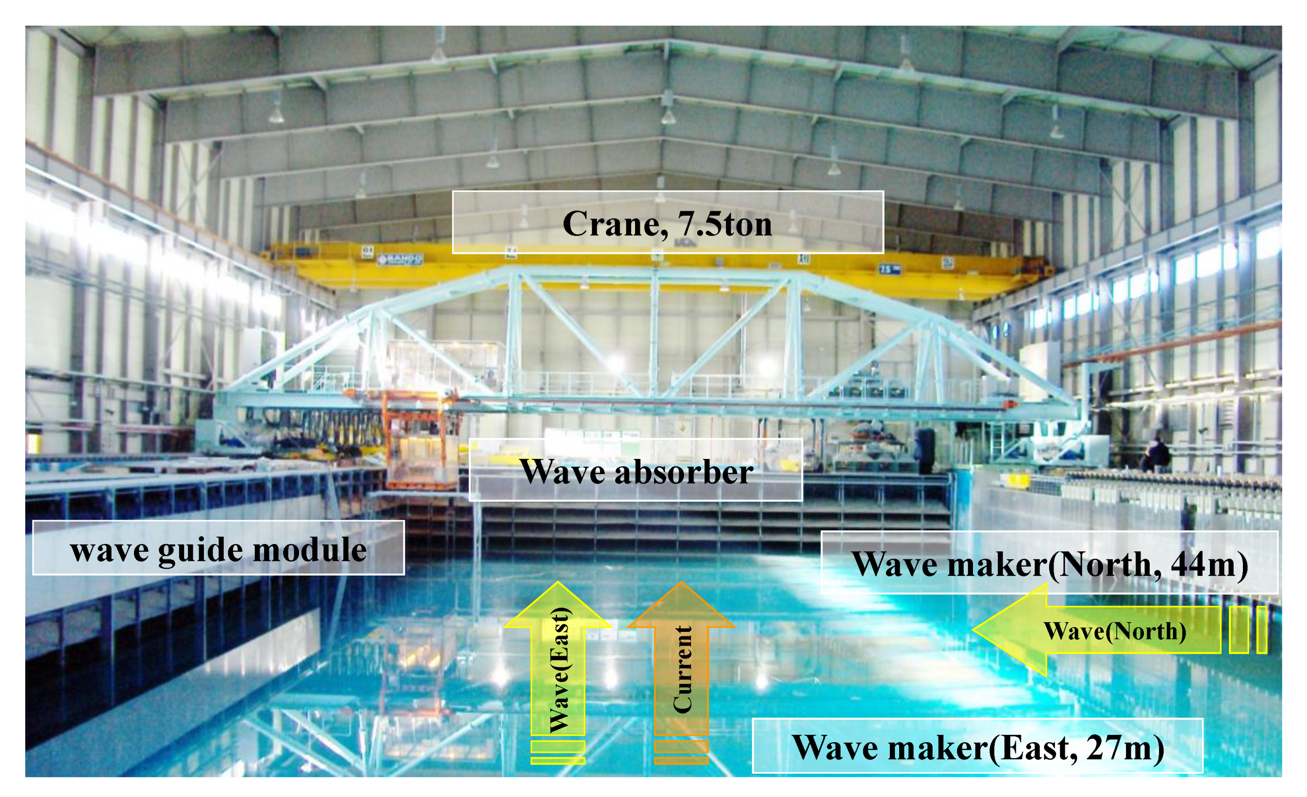
To validate the developed program, we performed an experimental test for offshore operation in the ocean engineering basin of the Korea Research Institute of Ships and Ocean Engineering (KRISO). The ocean engineering basin is 56 × 30 × 4.5 m and is equipped with a wave generator capable of regular, irregular and multidirectional waves, a current generator, and a wind generator as shown in Figure 14. For this experimental test, two floating crane models scaled to 1:40 were prepared. Detailed specification of the crane model is shown in

Table 2. Specification of crane model.

Item	Unit	1200-ton Model	2000-ton Model
Length Over All	[m]	2.250	2.250
Breadth	[m]	0.900	0.900
Depth	[m]	0.300	0.300
Draft	[m]	0.100	0.125
Displacement	[m3]	0.153	0.199
Weight of Crane on Deck	[kg]	59.600	59.600
Longitudinal Center of Buoyancy from Midship [FWD+]	[m]	0.000	0.000
Vertical Center of Buoyancy from keel line	[m]	−0.949	−0.949
Water Plan Area	[m2]	1.769	1.895
Longitudinal Center of Gravity from Midship [FWD+]	[m]	0.000	0.000
Vertical Center of Gravity from keel line	[m]	0.229	−0.949
GM (Metacenter Height)	[m]	0.285	0.610

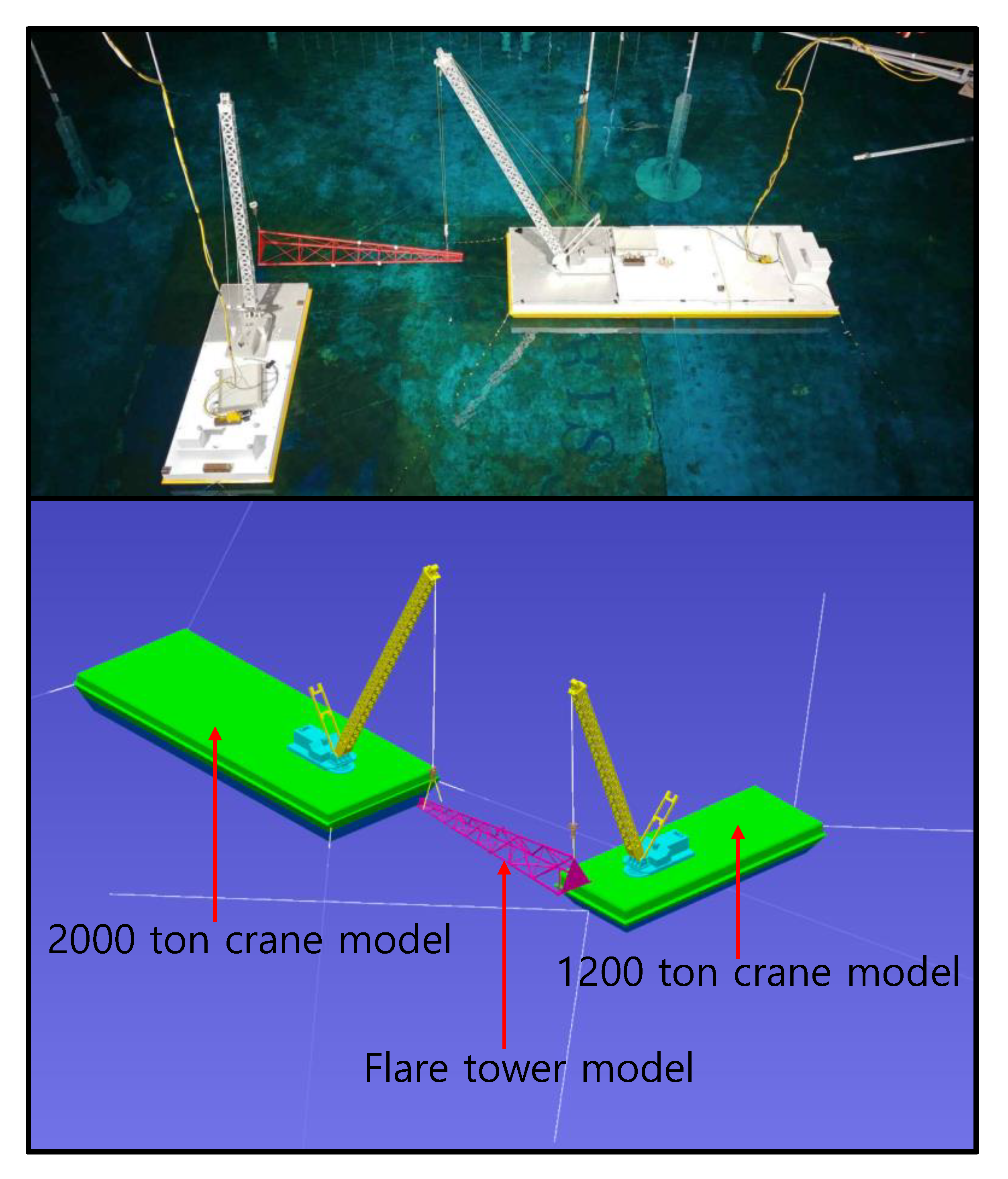
. Two floating crane models and one pile model were used to conduct operation of uprighting flare towers. Figure 15 shows a scene of the model test. A 1200-ton floating crane was moored with a spring type mooring line; on the other hand, 2000-ton floating crane was moored with a catenary type mooring line. For more accurate performance verification of pure mooring line and crane dynamics analysis, this experiment was conducted under the sea state 0 condition—the so called calm water condition.

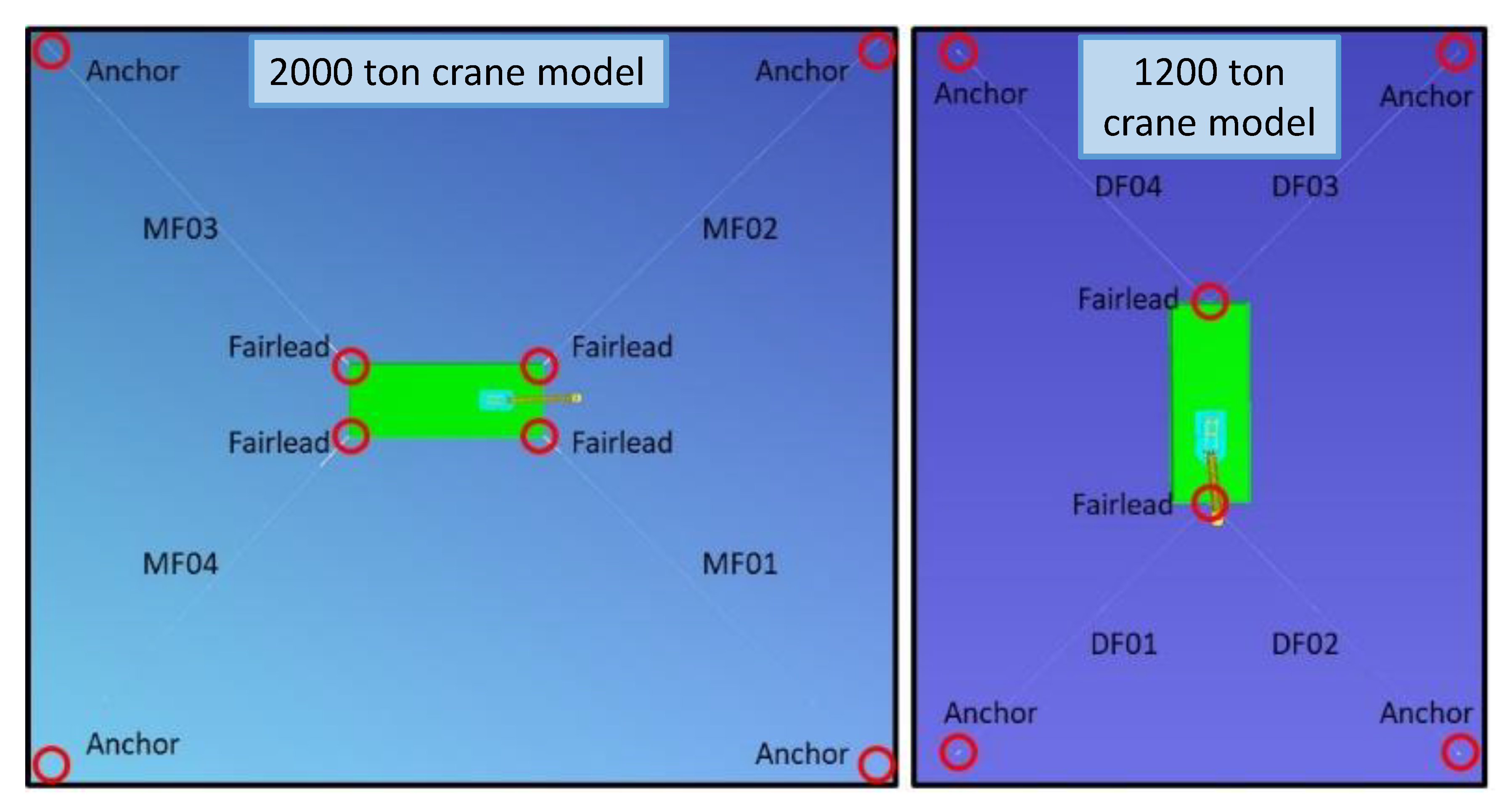
Figure 16 shows mooring points for the 1200-ton and 2000-ton crane models. The mooring coordinates of each crane model are listed in

Table 3. Mooring coordinates.

	Fairlead			Anchor
	x [m]	y [m]	z [m]	x [m]	y [m]	z [m]
MF01	1.632	−0.6	0.08	4.525	−6.625	−3.2
MF02	1.632	0.6	0.08	4.525	6.625	−3.2
MF03	−1.632	−0.6	0.08	−10.725	6.625	−3.2
MF04	−1.632	0.6	0.08	−10.725	−6.625	−3.2
DF01	1.125	0.0	0.05	3.8284	−2.6534	0.0
DF02	−1.125	0.0	0.05	3.8284	5.2534	0.0
DF03	−1.125	0.0	0.05	−1.8284	5.2534	0.0
DF04	1.125	0.0	0.05	−1.8284	−2.6534	0.0

. Positions of fairlead and anchor are expressed based on local coordinate system and global coordinate system, respectively.

The connection points of the mooring lines are listed in Table 3. The properties and pretension details of each mooring line for 1200-ton crane are as follows.

• Spring constant: 15.625 N/m.
• Pretension: 8.24 N.

The properties and pretension details of each mooring line for 2000-ton crane are as follows.

• Weight: 0.304 kg/m.
• Total length: 9.55 m.
• EA: 4040 N.
• Pretension: 24.515 N.

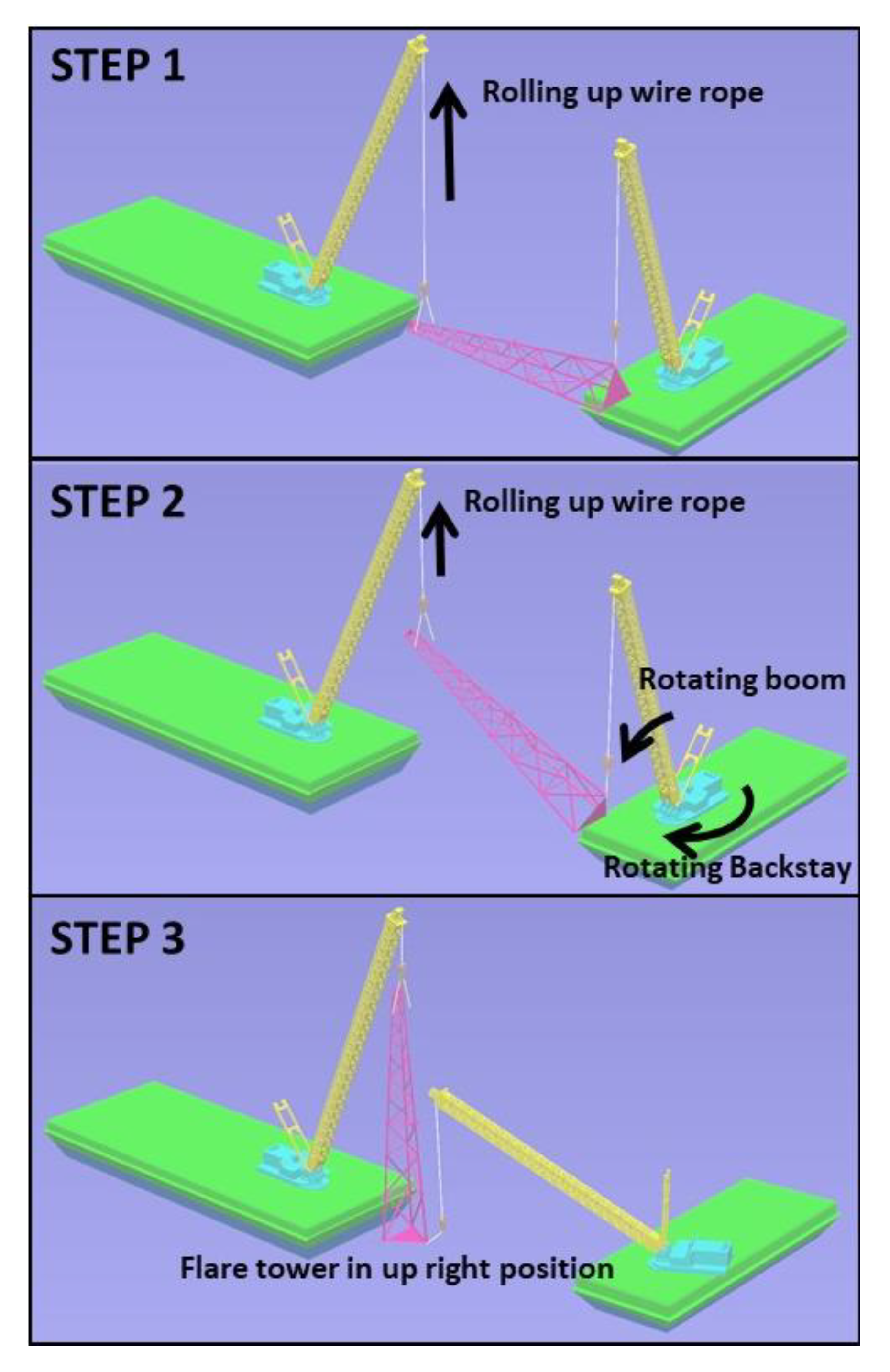
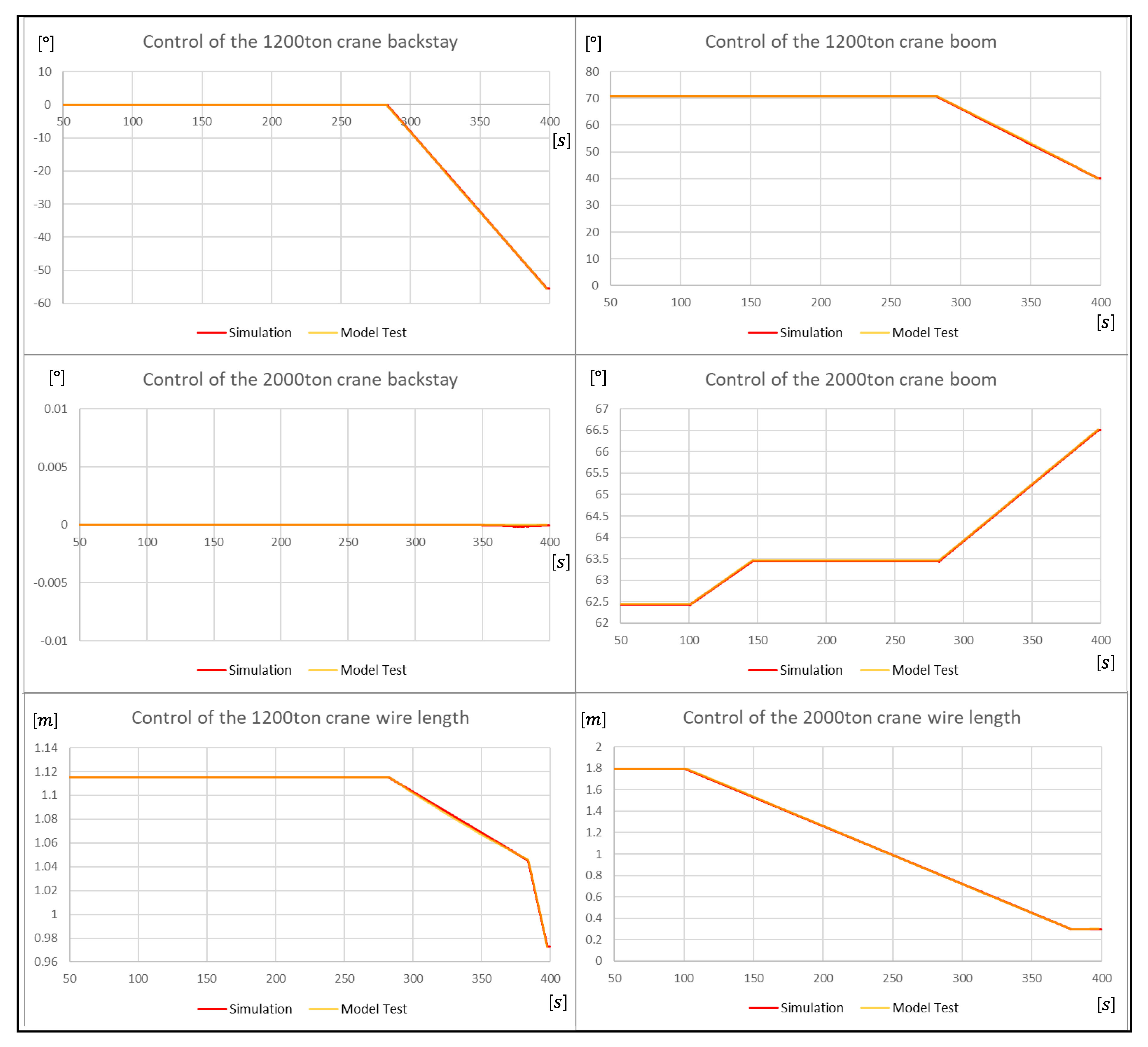
The procedure of the model test is shown in Figure 17. Figure 18 shows the control input values for the model test and simulation. The 1200-ton crane’s backstay and boom started to control at 280 s, the 2000-ton crane’s backstay did not rotate and the boom started to rotate at 100 and 280 s. The 1200-ton crane wire started to control at 270 s and the 2000-ton crane wire started at 100 s.

The control input values of the simulation and the model test were matched, and the motion of the flare tower, hoisting wire rope tension, and mooring line tension were compared.

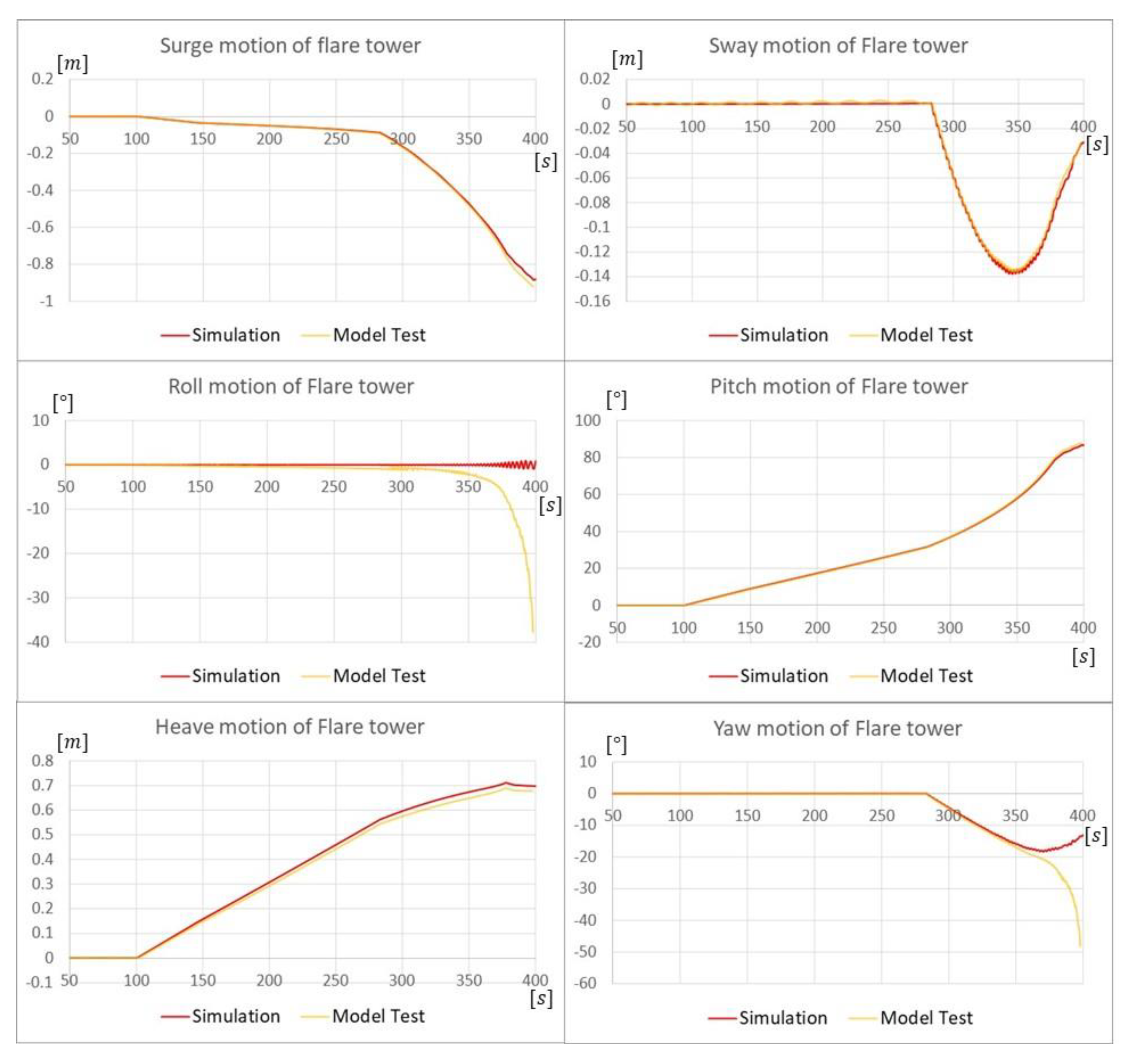
Figure 19 shows a comparison of the motion of the flare tower. The yellow and red lines represent the results of the model test and simulation, respectively. The trends of model tests and simulations were similar. In the case of surge motion, as it was erected, the flare tower moved in the direction of the 2000-ton crane. In the case of sway motion and yaw motion, the flare tower moved out of the center and then came back while the backstay of the 1200-ton crane was rotating. Roll motion rarely occurred. Since it is an erect work, the pitch angle and heave elevation increased. In the case of the model test, the roll and yaw motions can be seen as measurement errors as the flare tower was erected after 350 s. The maximum error rate between simulation and model test was 0.56% for surge, 0.19% for sway, 1.14% for heave, 5.72% for roll, 0.23% for pitch, and 0.34% for yaw.

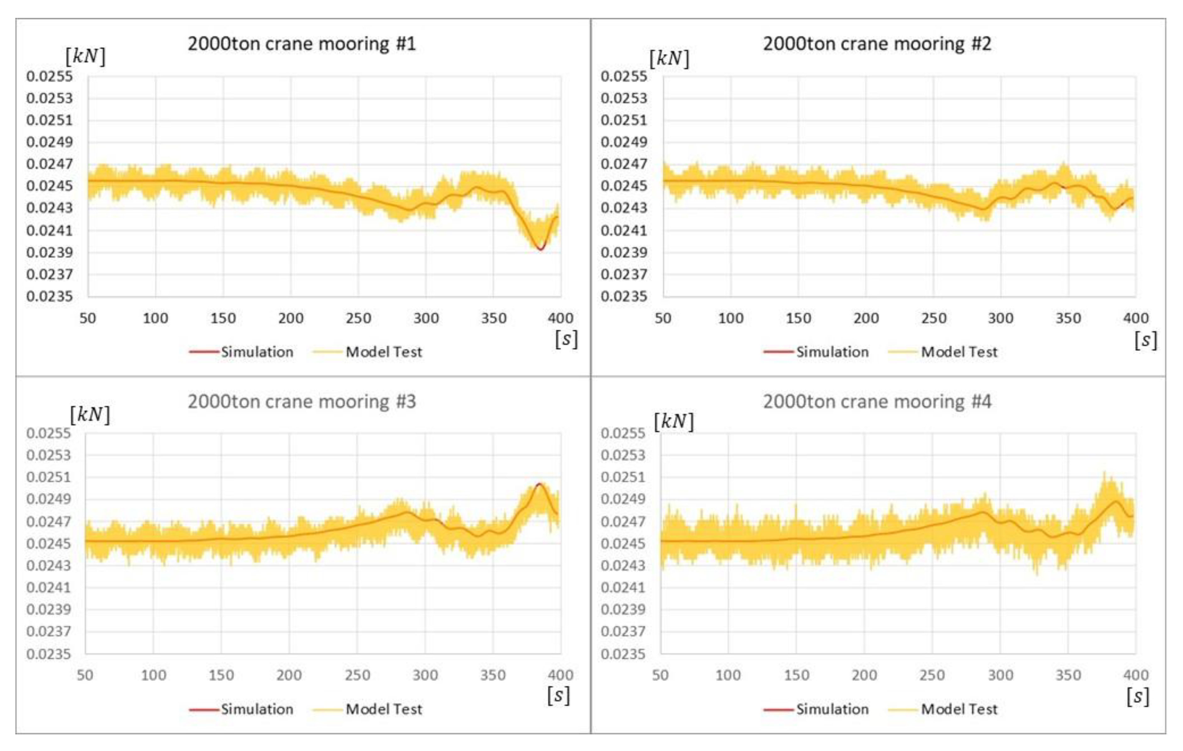
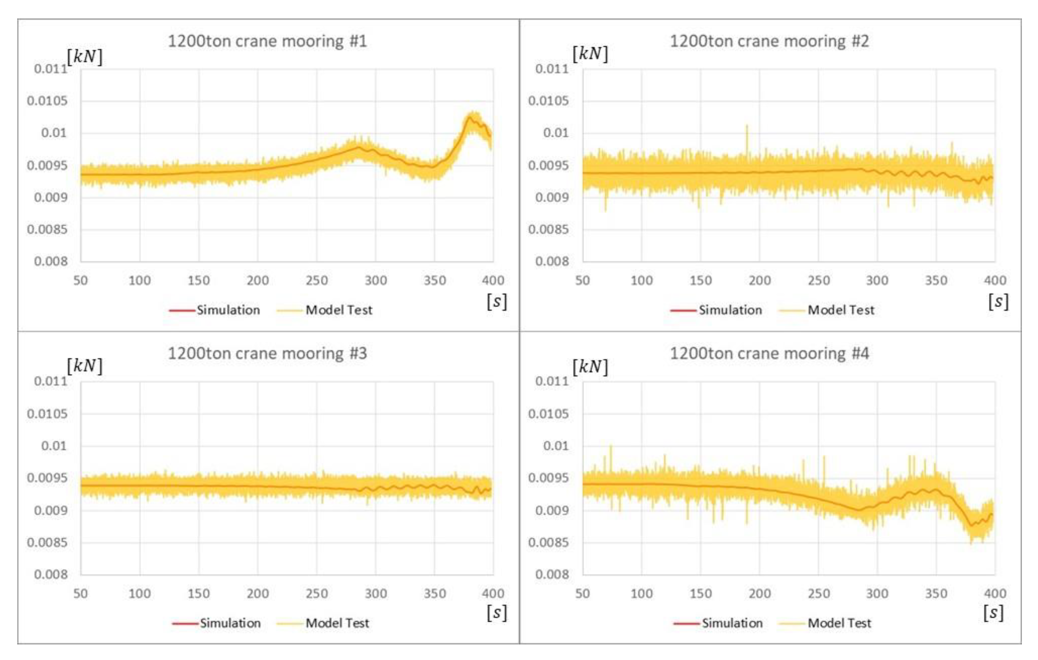
Figure 20 and Figure 21 show the comparison between the model test and the simulation of the mooring forces. The yellow and red lines represent the results of the model test and simulation, respectively. The trends for the variation in the mooring tension of the mooring lines of the simulation and the model test are similar.

In addition, the maximum error rate for the mooring line of the 2000-ton crane and was 3.9%, and the maximum error rate for the mooring line of the 1200-ton crane was 4.7%. The error rate was calculated by dividing the error of the mean absolute deviation between simulation and model test by the maximum amplitude. This error rate, which was less than 5%, shows the reliability and validity of the simulation results.

The free decay test in the model experiment was performed to obtain the natural period of the floating crane. In the case of the 2000-ton crane, the natural period was 18.11 s for surge, 19.81 s for sway, 1.36 s for roll, 1.60 s for pitch and 12.56 s for yaw. In the case of a 1200-ton crane, the natural period is 13.41 s for surge, 14.73 s for sway, 1.38 s for roll, 1.25 s for pitch and 7.69 s for yaw. In the case of heave motion, it was difficult to measure because the damping was too large. As shown in Figure 20, the tension of the 2000-ton crane vibrates for a period of approximately 20 s, which is the natural frequency of the 2000-ton crane model. Akin to the general model test, the operation was started in static equilibrium in this experiment. However, it was not easy to maintain a perfect static equilibrium in actual experiments. Due to this, very small natural vibration was measured, but the value was not large and did not significantly affect the experimental results. This phenomenon did not occur in the simulation because the initial state of the simulation was static equilibrium.

In addition, the amplitudes of the mooring tension in the model test and simulation are different, which is a limitation of the resolution performance of the measurement equipment.

6. Conclusions

A few programs are available for the multibody analysis of offshore operations, such as installation using a multicrane, considering catenary mooring analysis. Therefore, the aim of this study was to develop a nonlinear mooring analysis code that can be applied to the floating multibody analysis code.

In this study, the equations of motion for calculating the mooring force connected to the multibody system were introduced. The multibody equations for floating cranes were derived from the equations of motion. The finite element method (FEM) was used to derive equations to solve the stretchable catenary problem of the mooring line.

To validate the developed program, we conducted an experimental test for offshore operation. For this experimental test, two floating crane models scaled to 1:40 were prepared. Two floating crane models and one pile model were used to conduct the operation of uprighting flare towers. During the model test, the motion of the floating cranes and tensions of the mooring lines were measured. By comparing the simulation results and the model test results, we confirmed an error rate of 5% or less in the case of the mooring line. Therefore, we confirmed that the developed mooring simulator could be effectively used for multifloating crane simulations.

References

1. Ku, N.K.; Ha, S.; Hwang, H.J.; Kim, K.S.; Lee, K.Y.; Roh, M.I. Program of scenario management for simulation of lifting block using crane. In Proceedings of the 24th International Offshore and Polar Engineering Conference, Busan, Korea, 15–20 June 2014; pp. 838–846. [Google Scholar]
2. Roh, M.I.; Ha, S.; Ku, N.K.; Ham, S.H. Multibody system dynamics simulator for design and production of ships and offshore plants. In Proceedings of the 28th Asian-Pacific technical exchange and advisory meetings on marine structures (TEAM), Istanbul, Turkey, 13–16 October 2014; pp. 481–494. [Google Scholar]
3. Kim, B.W.; Sung, H.G.; Hong, S.Y.; Jung, H.J. Finite element nonlinear analysis for catenary structure considering elastic deformation. Comput. Model. Eng. Sci. 2010, 63, 29–45. [Google Scholar]
4. Garrett, D.L. Coupled analysis of floating production systems. Ocean Eng. 2005, 32, 802–816. [Google Scholar] [CrossRef]
5. Kim, B.W.; Hong, S.Y.; Hong, S.W. Extreme response analysis of moored body using combined design wave. J. Ships Ocean Eng. 2013, 52, 35–41. [Google Scholar]
6. Kim, B.W.; Sung, H.G.; Kim, J.H.; Hong, S.Y. Comparison of linear spring and nonlinear FEM methods in dynamics coupled analysis of floating structure and mooring system. J. Fluids Struct. 2013, 42, 205–227. [Google Scholar] [CrossRef]
7. Ham, S.H.; Roh, M.I.; Lee, H.; Ha, S. Multibody dynamic analysis of a heavy load suspended by a floating crane with constraint-based wire rope. Ocean Eng. 2015, 109, 145–160. [Google Scholar] [CrossRef]
8. Cha, J.H.; Ha, S.; Bae, J.H.; Cho, D.Y.; Shim, C.S.; Song, H.C. Dynamic analysis of offshore structure installation operation using dual floating cranes based on multibody system dynamics. In Proceedings of the 26th International Ocean and Polar Engineering Conference, Rhodes, Greece, 26 June–2 July 2016; pp. 880–885. [Google Scholar]
9. Yamamoto, T.; Yoshida, A.; Ijima, T. Dynamics of elastically moored floating objects. Appl. Ocean Res. 1980, 2, 85–92. [Google Scholar] [CrossRef]
10. Tang, H.J.; Huang, C.C.; Chen, W.M. Dynamics of dual pontoon floating structure for cage aquaculture in a two-dimensional numerical wave tank. J. Fluids Struct. 2011, 27, 918–936. [Google Scholar] [CrossRef]
11. Gutiérrez-Romero, J.E.; García-Espinosa, J.; Serván-Camas, B.; Zamora-Parra, B. Non-linear dynamic analysis of the response of moored floating structures. Mar. Struct. 2016, 49, 116–137. [Google Scholar] [CrossRef] [Green Version]
12. Shabana, A.A. Computational Dynamics; John Wiley & Sons, Inc.: Hoboken, NJ, USA, 1994. [Google Scholar]
13. Shabana, A.A. Dynamics of Multibody Systems, 3rd ed.; Cambridge University Press: Cambridge, UK, 2005. [Google Scholar]
14. Wang, L.; Kolios, A.; Cui, L.; Sheng, Q. Flexible multibody dynamics modelling of point-absorber wave energy converters. Renew. Energy 2018, 127, 790–801. [Google Scholar] [CrossRef]
15. Cha, J.H.; Roh, M.I.; Lee, K.Y. Dynamic response simulation of a heavy cargo suspended by a floating crane based on multibody system dynamics. Ocean Eng. 2010, 37, 1273–1291. [Google Scholar] [CrossRef]
16. Arbabi, F. Structural Analysis and Behavior; McGraw-Hill: New York, NY, USA, 1991. [Google Scholar]
17. Ku, N.K.; Cha, J.H. A study on moored floating body using non-linear FEM analysis. In Proceedings of the PACOMS (Pacific-Asia Offshore Mechanics Symposium), Gold Coast, Australia, 4–7 October 2016. [Google Scholar]
18. OrcaFlex Manual. 2019. Available online: https://www.orcina.com/webhelp/OrcaFlex/Default.htm (accessed on 20 November 2019).
Figure 1. Simulation program for dynamic analysis of offshore operation.
Jmse 09 00344 g001
Figure 2. Interface design between mooring analysis module and multibody motion equation module.
Jmse 09 00344 g002
Figure 3. Numerical example of mooring line.
Jmse 09 00344 g003
Figure 4. Comparison between analytical solution and simulation results obtained using the developed program.
Jmse 09 00344 g004
Figure 5. Results for static analysis of mooring line when q is 0°.
Jmse 09 00344 g005
Figure 6. Results for static analysis of mooring line when q is 20°.
Jmse 09 00344 g006
Figure 7. Result for static analysis of mooring line when q is 40°.
Jmse 09 00344 g007
Figure 8. Results for static analysis of mooring line when q is 60°.
Jmse 09 00344 g008
Figure 9. Results for static analysis of mooring line considering seabed condition when q is 20°.
Jmse 09 00344 g009
Figure 10. Results for static analysis of mooring line considering seabed condition when q is 40°.
Jmse 09 00344 g010
Figure 11. Results for static analysis of mooring line considering seabed condition when q is 60°.
Jmse 09 00344 g011
Figure 12. Conditions of the first simulation for forced oscillation body with two mooring lines.
Jmse 09 00344 g012
Figure 13. Restoring force for examples of pulling tests.
Jmse 09 00344 g013
Figure 14. Ocean engineering basin of the Korea Research Institute of Ships and Ocean Engineering (KRISO).
Jmse 09 00344 g014
Figure 15. Scene of model test and simulation.
Jmse 09 00344 g015
Figure 16. Mooring points of model test.
Jmse 09 00344 g016
Figure 17. Procedure of model test.
Jmse 09 00344 g017
Figure 18. Comparison of model test and simulation control values.
Jmse 09 00344 g018
Figure 19. Comparison of flare tower motion.
Jmse 09 00344 g019
Figure 20. Tension of mooring lines for 2000-ton crane model.
Jmse 09 00344 g020
Figure 21. Tension of mooring lines for 1200-ton crane model.
Jmse 09 00344 g021